Knowledge Transfer For On-Device Speech Emotion Recognition
with Neural Structured Learning

Abstract

Speech emotion recognition (SER) has been a popular research topic in human-computer interaction (HCI). As edge devices are rapidly springing up, applying SER to edge devices is promising for a huge number of HCI applications. Although deep learning has been investigated to improve the performance of SER by training complex models, the memory space and computational capability of edge devices represents a constraint for embedding deep learning models. We propose a neural structured learning (NSL) framework through building synthesized graphs. An SER model is trained on a source dataset and used to build graphs on a target dataset. A relatively lightweight model is then trained with the speech samples and graphs together as the input. Our experiments demonstrate that training a lightweight SER model on the target dataset with speech samples and graphs can not only produce small SER models, but also enhance the model performance compared to models with speech samples only and those using classic transfer learning strategies.

Index Terms—  Speech emotion recognition, neural structured learning, edge device, lightweight deep learning

1 Introduction

Speech emotion recognition (SER), which aims to recognise emotional states from speech, has been a popular research topic in the domain of human-computer interaction (HCI) [1]. SER has been applied to a range of applications, including call centres, education, mental health, computer games, and many others [2]. In particular, speech signals provide rich and complementary information to other modalities, e. g., images, biosignals, social media, etc [3]. SER can not only improve the performance of emotion recognition when combined with other modalities in a multimodal system, but also enable machines to perceive human emotions when other modalities are not available, such as in audio-only call centres [1].

Deep learning has been widely applied to SER with many model architectures, including spectrum-based and end-to-end models. Spectrum-based models process spectrum features from speech signals [4, 5], while end-to-end models directly process raw speech signals [6, 7]. Convolutional neural networks (CNNs), recurrent neural networks (RNNs), and their variants (e. g., transformers) have been commonly used to build either end-to-end or spectrum-based models for SER [8, 9].

Improving the performance of SER faces two challenges. First, creating emotional speech datasets with high-quality annotations is a time-consuming and potentially biased process, leading to small-scale datasets [10]. Second, with the increasing demand for SER in Internet-of-Things (IoT) applications, it is essential to train lightweight neural networks for efficient model development. However, directly fine-tuning complex SER models pre-trained on large-scale data places a high demand on computing systems [11].

More recently, neural structured learning (NSL) was proposed to add structured signals (e. g., graphs) as the model input in addition to the original data [12]. In particular, NSL was developed to solve the data labelling problem of semi-supervised learning, and to build adversarial training against adversarial attacks [12]. Inspired by NSL, it is promising to construct a graph with a pre-trained model to break the bottleneck caused by small-scale labelled data and edge devices.

In this study, we propose an NSL framework to transfer the knowledge of a large, pre-trained SER model to a smaller model with graph. To the best of the authors’ knowledge, there were only few studies using NSL for SER [13]. The contributions of our work are twofold: i) transferring model knowledge through an NSL-generated graph can improve performance by leveraging multiple databases; ii) the proposed NSL framework can train lightweight neural networks without a high requirement of computing resources. Evaluated on an emotional speech dataset, our NSL framework outperforms models trained on the original data only and those trained with classic transfer learning strategies.

Related Works. Deep Learning for SER. As previously mentioned, deep learning is mainly applied for SER with spectrum-based and end-to-end models. Spectrum-based models are typically shallower and more efficient than end-to-end models due to smaller data size of extracted spectrums compared to raw speech signals. On the other hand, end-to-end models save the time of selecting suitable spectrum types and can extract complementary features over fixed spectrums. An end-to-end model was developed based on 1D CNNs for learning spatial features in SER [14]. Additionally, stacked multiple transformer layers were utilised in [8] to better extract global feature dependencies from speech. More recently, wav2vec models, which include CNNs and transformers, were trained with self-supervised learning on unlabelled speech data [15]. Wav2vec models have been applied to generate speech embeddings for SER [16, 17].

Transfer Learning. Transfer learning was designed to transfer knowledge learnt from a large-scale source dataset to a smaller target dataset for better performance in an efficient manner [18]. Transfer learning has been applied to SER due to limited labelled emotional speech data. For instance, a source dataset with a large number of languages was utilised along with a small amount of target data for training deep belief networks in [19]. Various approaches to transfer learning aim to gap the data distribution difference between the source dataset and the target dataset [18]: instance-based transfer learning achieves this by re-weighting samples in the source dataset during training; feature-based transfer learning attempts to learn new feature representations from original ones; parameter-based transfer learning targets to find shared model parameters between the source domain and the target domain; relational knowledge transfer learning works on relational domains with non-i.i.d. data and builds mapping of relational knowledge [18]. These transfer learning strategies mostly (instance-based, parameter-based, and relational ones) require training one or two models with the same architecture on both source and target data. The proposed knowledge transfer via the NSL framework is an extension of feature-based transfer learning. Compared with the transferred representations, the additional graphs fed into the model on the target data have more regularised and complementary information.

Neural Structured Learning. Neutral Structured Learning (NSL) adds additional structured signals (e. g., graghs) as a regularisation term to maintain the latent structural similarity among input signals. In [13], Mel frequency cepstrum coefficients and NSL-generated structured signals were combined for SER. However, there was no knowledge transfer in that work and the type of structured signals were not clearly specified.

2 Methodology

As depicted in Figure 1, with the help of a model trained on a related emotional source speech dataset, embeddings of audio samples in the target dataset are extracted and then used to construct graphs accordingly. Log Mel spectrograms of the audio samples, along with the graphs, are fed into a relatively lightweight model. Afterwards, for each training sample, the loss function has two parts: (1) the neighbor loss, which reduces the distance between the embedding of a sample and the embeddings of its neighbors to maintain structural similarity, and (2) the supervised loss, which is calculated based on the predicted label and the true label in supervised learning.

2.1 Upstream and Downstream Models

The upstream model denotes a large pre-trained model on a source dataset in SER, while the downstream model on the target data is lightweight and possibly run on edge devices. As noted in Section 1, spectrum-based models can be smaller than end-to-end models due to different inputs. Therefore, the upstream model is an end-to-end model and the downstream one is a spectrum-based model herein.

Upstream. Due to its powerful capability for representations extraction, the upstream model utilised herein is wav2vec 2.0 [15], which has been widely applied in SER [16, 20, 21]. Wav2vec 2.0 is an end-to-end model composed of a CNN module as the latent speech feature encoder and a Transformer module for capturing global contextual dependencies. The output of the encoder module is discretised with product quantisation [22] for self-supervised training. The pre-trained wav2vec 2.0 model applied in this work is trained on the 960-hour Librispeech corpus [23]. An audio classification head is then added with two linear layers for the SER task. After fine-tuning the pre-trained wav2vec 2.0 model on the source dataset, it becomes the aforementioned upstream model.

Downstream. Compared to raw audio signals, the extracted log Mel spectrograms require less storage space. Several representative lightweight downstream CNN models on the target dataset are selected: VGG-15, ResNet-9, and CNN-6, whose parameter numbers are 14.86 M, 4.96 M, and 4.44 M, respectively. However, the wav2vec 2.0 model has over 90.37 M parameters, making the above downstream models relatively lightweight.

2.2 Neural Structured Learning

With graphs as the structured signals, NSL maintains the structural similarity between the speech samples. In this way, NSL has the potential to improve the model performance with a low requirement of computational resource during training the downstream model.

2.2.1 Graph

The input to the downstream model includes data nodes $D$ and the graph $G$. Specifically, $D=\{(x_{i},y_{i})\},i=1,...,N$, where $x_{i}$ is a data sample, $y_{i}$ is its emotional state, and $N$ is the number of training samples; The graph $G=(D,E)$, where $E$ denotes the bi-directional edges connecting similar nodes. A pair of connected nodes in $G$ is a neighbour of each other $\mathcal{N}=(x_{i},x_{j}),i\neq j$. The neighbours of $x_{i}$ are computed by

$$\{x_{k}|S(h(x_{i}),h(x_{k}))>\epsilon,\ k=1,...,N\ \mbox{and}\ k\neq i\},\vspace{-5pt}$$ (1)

where $S$ is the cosine similarity, and $h$ is the feature embedding extracted by the upstream model. The graph $G$ with structured similarity information is then fed into the current lightweight downstream model to achieve the knowledge transfer.

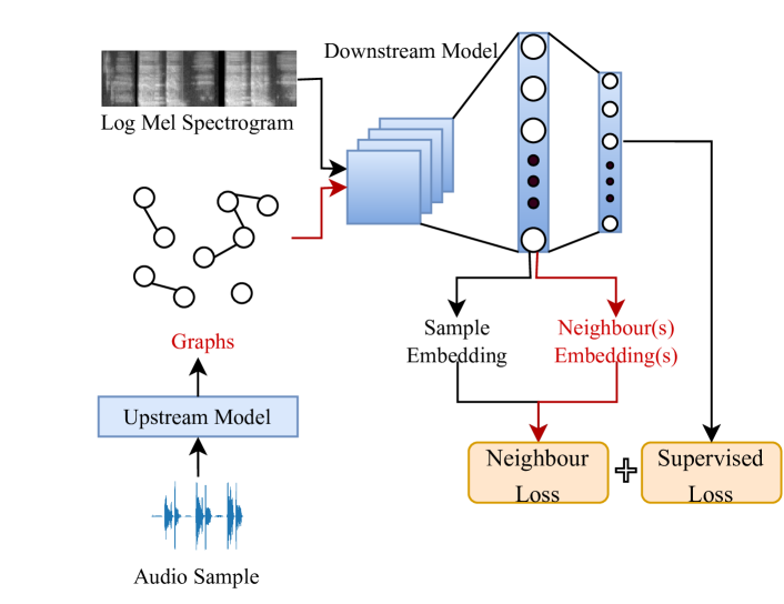
Fig. 1: The framework of the applied NSL for SER. Graphs act as structured signals and, along with log Mel spectrograms, are fed into a downstream lightweight model. The final loss function is the weighted sum of neighbour loss and supervised loss.

2.2.2 Loss Function

The loss function applied in this work is the weighted sum of two components, supervised loss and neighbour loss, as follows:

$$\mathcal{L}= \sum_{i=1}^{N}\mathcal{L}_{\mbox{supervised}}(y_{i},\hat{y}_{i})+\alpha\sum_{i=1}^{N}\sum_{\{x_{k}\}}\mathcal{L}_{\mbox{neighbour}}(p(x_{i}),p(x_{k})),$$ (2)

where $\mathcal{L}_{\mbox{supervised}}$ is calculated by the cross entropy loss function for classification based on the target $y$ and predicted $\hat{y}$; $\mathcal{L}_{\mbox{neighbour}}$ reflects the distance between the embeddings $p(x_{i})$ and $p(x_{k})$ from the intermediate layers of the downstream model. We use $(1-\mbox{cosine}\ \mbox{similarity})$ as the distance function and $\alpha$ is a multiplier.

By minimising the neighbour loss, the similarity among a sample and its neighbours is maintained. As a result, the transferred knowledge from the source dataset is used on the target dataset.

3 Experiments

3.1 Databases

RAVDESS. The Ryerson Audio-Visual Database of Emotional Speech and Song (RAVDESS) is a multi-modal English dataset containing 1,440 speech recordings. It was recorded from 24 professional actors (12 females and 12 males) and labelled into eight emotional classes: angry, calm, disgusted, fearful, happy, neutral, sad, surprised. Each emotional class has eight recordings from each speaker, except for neutral, which has four. We split the dataset in a speaker-independent and gender-balanced manner shown in Table 1.

Besides its wide applications in SER [2], the reasons why we choose RAVDESS as the source dataset are that it is recorded from professional actors in a well-controlled environment, its emotional labels have high levels of validity, and the dataset is gender-balanced.

Table 1: Split details of the source dataset RAVDESS.

# Train Val Test $\bm{\sum}$ F / M Speaker 10 8 6 24 12 /   12 $\bm{\sum}$ 600 480 360 1,440 720 / 720

DEMoS. The Database of Elicited Mood in Speech (DEMoS) [24] is an Italian speech corpus with $7.7$ hours of audio samples recorded from $68$ speakers (45 males and 23 females). Besides the $332$ neutral speech recordings, there are in total $9,365$ audio samples annotated into seven classes: anger, disgust, fear, guilt, happiness, sadness, and surprise. Similar to prior work [25] on the DEMoS data, the minority neutral class is not considered and the remaining $9,365$ emotional speech samples are divided into 40 % train, 30 % validation, and 30 % test sets with speaker-independent strategy. The detailed data distribution of the DEMoS is depicted in Table 2.

Table 2: Emotion distribution of the target dataset DEMoS dataset.

# Train Val Test $\bm{\sum}$ F / M Speaker 27 25 16 68 23 /      45 Anger 586 531 360 1,477 400 /    729 Disgust 666 608 404 1,678 596 / 1,082 Fear 461 404 291 1,156 524 /    871 Guilt 453 395 281 1,129 415 /    741 Happiness 561 471 363 1,395 516 /    961 Sadness 606 543 381 1,530 349 /    651 Surprise 396 358 246 1,000 532 /    998 $\bm{\sum}$ 3,729 3,310 2,326 9,365 3,332 / 6,033

3.2 Experimental Settings

Evaluations Metrics. Similar to previous works on the DEMoS, the Unweighted Average Recall (UAR) is utilised as the standard evaluation metric to mitigate the class imbalance issue. For the RAVDESS, accuracy is applied to better compare with other works [26, 27, 28, 29].

Implementation Details. In our experiments, all audio recordings are re-sampled into $16$ kHz. The batch size is $16$. For the upstream wav2vec 2.0 model fine-tuned on the RAVDESS, the fine-tuning procedure is optimised by an Adam optimiser with a learning rate of $3e-5$, and stopped after $20$ epochs. The feature encoder of wav2vec 2.0 is frozen. The outputs of the second last fully connected layer ‘FC1’ of the wav2vec 2.0 model are averaged over the time frame, resulting in the embeddings $h$. The dimension of $h(x_{i})$ is $256$, and we set the threshold $\epsilon$ as $0.99$. A lager max number of neighbors $n$ requires more computing resources on edge devices; therefore, we limit $n$ to under 10 considering the dataset size of the DEMoS. For ablation study, we choose 3, 6, and 9 for $n$. Similarly, we empirically chose 0.01, 0.1 and 1 for the multiplier $\alpha$.

As for the downstream lightweight models development, log Mel spectrograms are extracted from the DEMoS audio samples as features. Firstly, we unify the audio length as the maximum one of all audio durations by simply cutting extra signals and self-repeating shorter samples. To extract log Mel spectrograms, the sliding window, overlap, and Mel bins are set as $512$, $256$, and $64$ time frames, respectively. In this way, the extracted log Mel spectrograms’ dimension is ($373$, $64$), where $373$ is on the time axis, and $64$ describes the number of Mel frequency bins. The model development is also optimised with an Adam optimiser with an initial learning rate of $1e-3$ and stopped after $50$ epochs. The learning rate decays by a factor of $0.9$ after every 5 epochs. As for the comparison with transfer learning, the same embeddings generated from the upstream wav2vec 2.0 model are added / maximised / averaged with the output of the ‘FC1’ layer of the downstream lightweight models. The code for this study has been made available at https://github.com/glam-imperial/NSL-SER.

3.3 Wav2Vec2 fine-tuning

To ensure the efficacy of NSL in constructing the graphs, we compare the performance of the fine-tuned wav2vec 2.0 model with state-of-the-art (SOTA) models on the RAVDESS. Accuracy is used to ensure a relatively fair comparison. Moreover, the eight emotional classes are balanced besides neutral, so accuracy is close to UAR. The SOTA models’ accuracy scores on the RAVDESS test dataset are $76.08$ % [26], $78.8$ % [27], $93.2$ % [28], and $81.94$ % [29]. Our fine-tuned wav2vec 2.0 model achieves $82.50$ % test accuracy, which is better than most works. Please note that the data split is different between SOTA’s works and our work. Specifically, data split ratio, strategy, and considered emotional classes are not the same.

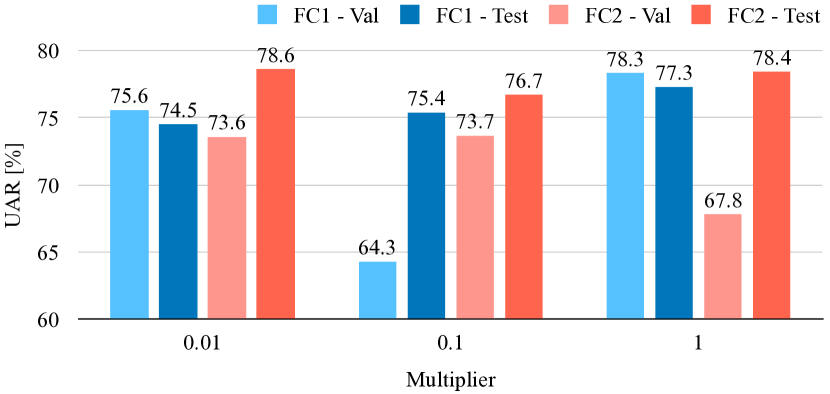
(a) # Neighbours = 3

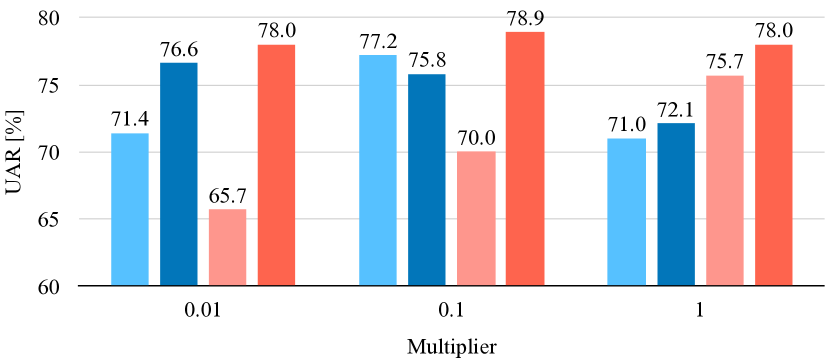
(b) # Neighbours = 6

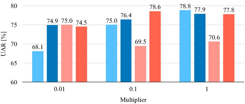
(c) # Neighbours = 9

Fig. 2: Comparison of the performance (UAR [%]) of the VGG-15 with NSL on the DEMoS validation and test datasets.

Table 3: Models’ performances [Accuracy / UAR  %] on DEMoS validation and test datasets. $n$: maximum neighbours, $\alpha$: multiplier.

VGG-15 ResNet-9 CNN-6 NN # $n$ $\alpha$ Val Test Val Test Val Test Base Model – – 71.0 / 66.4 84.0 / 77.2 79.4 / 73.9 81.7 / 74.6 68.4 / 65.3 80.7 / 73.1 Transfer Learning (Add) – – 70.9 / 66.7 80.9 / 74.0 78.5 / 73.2 82.4 / 75.2 80.6 / 74.7 82.0 / 75.2 Transfer Learning (Max) – – 76.3 / 70.1 75.1 / 68.5 80.3 / 74.9 81.1 / 74.5 74.2 / 67.8 76.0 / 70.0 Transfer Learning (Avg) – – 70.0 / 63.8 74.3 / 66.4 82.0 / 76.8 82.5 / 75.1 80.5 / 74.8 81.6 / 74.0 3 0.01 80.3 / 73.6 86.0 / 78.6 78.3 / 73.0 83.8 / 76.3 78.2 / 72.6 84.2 / 77.0 NSL 6 0.1 74.9 / 70.0 85.9 / 78.9 74.5 / 67.8 81.6 / 74.5 80.7 / 74.9 83.1 / 76.0 9 0.1 75.4 / 69.5 86.3 / 78.6 74.8 / 68.5 83.0 / 76.2 77.8 / 73.0 84.1 / 76.9

3.4 Results and Sensitivity Analysis

As shown in Figure 2, we evaluate the performance of VGG-15 models in different NSL settings, i. e., different maximum neighbours $n$ and two embedding layers (‘FC1’, ‘FC2’) for building graphs. Compared with the performance of base VGG-15 (validation UAR $66.4$ % , test UAR $77.2$ %), VGG-15 with NSL achieves better performance. Specifically, when $n$ is 6, $\alpha$ is 0.1, and the embedding layer is ‘FC2’, the test UAR obtains significant improvement ($p<0.1$ in a one-tailed z-test). To further validate the effectiveness of the proposed NSL framework, we choose the best settings for $n$, $\alpha$, and embedding layer based on the test UAR indicated in Figure 2. Specifically, by averaging and comparing the test UAR grouped by ‘FC1’ and ‘FC2’, we observe that ‘FC2’ tends to obtain better performance, possibly due to more abstract representations learnt after ‘FC2’. Afterwards, for different $n$ (i. e., 3, 6, 9), we find the best multipliers are 0.01, 0.1, and 0.1, respectively. With more neighbours, stronger structural similarities among inputs are obtained, and the neighbour loss may play a more crucial role during model training with larger multiplier values. It further validates the efficacy of the proposed NSL framework. The following experiments are conducted with lightweight models with these settings.

Performances of VGG-15, ResNet-9, and CNN-6 on the DEMoS are presented in Table 3, where the ‘Base Model’ refers to the model trained solely on log Mel spectrograms. On both accuracy and UAR, NSL models almost outperform base models. Specifically, when $n$ is 3 and $\alpha$ is $0.01$, test UARs of ResNet-9 (76.3 %) and CNN-6 (77.0 %) significantly improve compared to their corresponding base models ($p<0.1$ and $p<0.002$ in one-tailed z-tests, respectively). Notably, for CNN-6, NSL substantially enhances almost all validation and test UARs, indicating significantly better performance. These results demonstrate NSL can help improve simple CNNs’ performance via knowledge transfer. Comparing with classic transfer learning strategies, NSL models also perform better. Specifically, test UARs of VGG-15 and CNN-6 are significantly better than those of transfer learning models ($p<0.001$ and $p<0.1$ in one-tailed z-tests, respectively). Figure  3 shows the class-wise analysis of best model VGG-15 with NSL on the DEMoS test dataset.

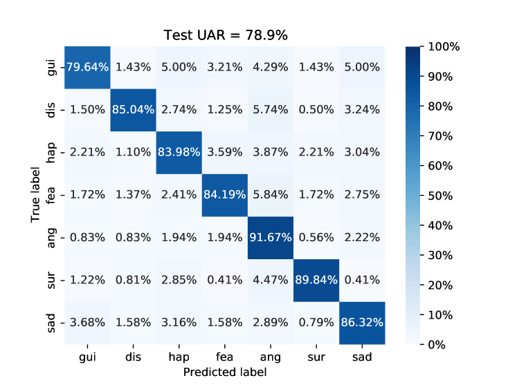
Fig. 3: Confusion matrix for the best VGG-15 under NSL framework on the DEMoS test dataset. ‘gui’: Guilt, ‘dis’: Disgust, ‘hap’: Happiness, ‘fea’: Fear, ‘ang’: Anger, ‘sur’: Surprise, ‘sad’: Sadness.

3.5 Discussion

With graphs maintaining the structural similarities among input signals, NSL enables performance improvement of lightweight models. However, it should be noted that some of the results in Table 3 are not stable, such as the validation UARs of ResNet-9 with NSL. This instability may be caused by the latent data difference between RAVDESS and DEMoS. Specifically, the DEMoS dataset contains speech in Italian, whereas samples in RAVDESS are in English; furthermore, the emotion classes of the two datasets are also different. When compared to the SOTA works on DEMoS [30], our work’s performance is comparable, which can be attributed to data split differences. However, we would like to emphasise that this work focuses on the performance improvement of lightweight models with the help of knowledge transfer by the NSL framework.

4 Conclusions and Future Work

This paper proposed a neural structured learning (NSL) framework to transfer the knowledge learnt from the related speech emotion dataset to the target one by maintaining the structural similarities defined in graphs. Specifically, a pre-trained upstream wav2vec 2.0 model was fine-tuned on the RAVDESS emotional speech database for graph construction on DEMoS; further experiments on the DEMoS emotional speech database with downstream lightweight models validated the effectiveness of our NSL framework.

In future work, a larger-scale source dataset (e. g., CMU-MOSEI [31]) can be applied as the source dataset and more target datasets can be also explored. Moreover, some domain adaptation strategies [32] can be explored to bridge the latent data difference between the source dataset and the target dataset.

References

- [1] Taiba Majid Wani et al., “A comprehensive review of speech emotion recognition systems,” IEEE Access, vol. 9, pp. 47795–47814, 2021.
- [2] Mehmet Berkehan Akçay and Kaya Oğuz, “Speech emotion recognition: Emotional models, databases, features, preprocessing methods, supporting modalities, and classifiers,” Speech Communication, vol. 116, pp. 56–76, 2020.
- [3] Ruhul Amin Khalil et al., “Speech emotion recognition using deep learning techniques: A review,” IEEE Access, vol. 7, pp. 117327–117345, 2019.
- [4] Siqing Wu, Tiago H. Falk, and Wai-Yip Chan, “Automatic speech emotion recognition using modulation spectral features,” Speech Communication, vol. 53, no. 5, pp. 768–785, 2011.
- [5] Ziping Zhao, Yiqin Zhao, Zhongtian Bao, Haishuai Wang, Zixing Zhang, and Chao Li, “Deep spectrum feature representations for speech emotion recognition,” in Proc. ASMMC-MMAC, Seoul, Korea, 2018, p. 27–33.
- [6] Puneet Kumar et al., “End-to-end triplet loss based emotion embedding system for speech emotion recognition,” in Proc. ICPR, Milan, Italy, 2021, pp. 8766–8773.
- [7] Panagiotis Tzirakis, Jiehao Zhang, and Bjorn W. Schuller, “End-to-end speech emotion recognition using deep neural networks,” in Proc. ICASSP, Calgary, AB, 2018, pp. 5089–5093.
- [8] Xianfeng Wang et al., “A novel end-to-end speech emotion recognition network with stacked transformer layers,” in Proc. ICASSP, 2021, pp. 6289–6293.
- [9] Jianfeng Zhao, Xia Mao, and Lijiang Chen, “Speech emotion recognition using deep 1D & 2D CNN LSTM networks,” Biomedical Signal Processing and Control, vol. 47, pp. 312–323, 2019.
- [10] Reza Lotfian and Carlos Busso, “Curriculum learning for speech emotion recognition from crowdsourced labels,” IEEE/ACM Transactions on Audio, Speech, and Language Processing, vol. 27, no. 4, pp. 815–826, 2019.
- [11] Victor Sanh, Thomas Wolf, and Alexander Rush, “Movement pruning: Adaptive sparsity by fine-tuning,” in Advances in Neural Information Processing Systems, 2020, vol. 33, pp. 20378–20389.
- [12] Arjun Gopalan et al., “Neural structured learning: Training neural networks with structured signals,” in Proc. WSDM, New York, NY, 2021, p. 1150–1153.
- [13] Md. Zia Uddin and Erik G. Nilsson, “Emotion recognition using speech and neural structured learning to facilitate edge intelligence,” Engineering Applications of Artificial Intelligence, vol. 94, pp. 103775, 2020.
- [14] Mustaqeem and Soonil Kwon, “MLT-DNet: Speech emotion recognition using 1D dilated CNN based on multi-learning trick approach,” Expert Systems with Applications, vol. 167, pp. 114177, 2021.
- [15] Alexei Baevski, Yuhao Zhou, Abdelrahman Mohamed, and Michael Auli, “wav2vec 2.0: A framework for self-supervised learning of speech representations,” Advances in Neural Information Processing Systems, vol. 33, pp. 12449–12460, 2020.
- [16] Leonardo Pepino, Pablo Riera, and Luciana Ferrer, “Emotion Recognition from Speech Using wav2vec 2.0 Embeddings,” in Proc. Interspeech, Brno, Czechia, 2021, pp. 3400–3404.
- [17] Heqing Zou et al., “Speech emotion recognition with co-attention based multi-level acoustic information,” in Proc. ICASSP, Singapore, 2022, pp. 7367–7371.
- [18] Sinno Jialin Pan and Qiang Yang, “A survey on transfer learning,” IEEE Transactions on Knowledge and Data Engineering, vol. 22, no. 10, pp. 1345–1359, 2010.
- [19] Siddique Latif, Rajib Rana, Shahzad Younis, Junaid Qadir, and Julien Epps, “Transfer learning for improving speech emotion classification accuracy,” in Proc. Interspeech, Hyderabad, India, 2018, pp. 257–261.
- [20] Mayank Sharma, “Multi-lingual multi-task speech emotion recognition using wav2vec 2.0,” in Proc. ICASSP, Singapore, 2022, pp. 6907–6911.
- [21] Edmilson Morais et al., “Speech emotion recognition using self-supervised features,” in Proc. ICASSP, Singapore, 2022, pp. 6922–6926.
- [22] Herve Jégou, Matthijs Douze, and Cordelia Schmid, “Product quantization for nearest neighbor search,” IEEE Transactions on Pattern Analysis and Machine Intelligence, vol. 33, no. 1, pp. 117–128, 2011.
- [23] Vassil Panayotov, Guoguo Chen, Daniel Povey, and Sanjeev Khudanpur, “Librispeech: an asr corpus based on public domain audio books,” in Proc. ICASSP. IEEE, 2015, pp. 5206–5210.
- [24] Emilia Parada-Cabaleiro, Giovanni Costantini, Anton Batliner, Maximilian Schmitt, and Björn Schuller, “DEMoS: An Italian emotional speech corpus,” Language Resources and Evaluation, pp. 1–43, Feb. 2019.
- [25] Zhao Ren, Jing Han, Nicholas Cummins, and Björn Schuller, “Enhancing transferability of black-box adversarial attacks via lifelong learning for speech emotion recognition models,” in Proc. INTERSPEECH, Shanghai, China, 2020, pp. 496–500.
- [26] Sibtain Ahmed Butt et al., “An improved convolutional neural network for speech emotion recognition,” in Proc. SCDM, Basel, Switzerland, 2022, pp. 194–201.
- [27] Suprava Patnaik, “Speech emotion recognition by using complex mfcc and deep sequential model,” Multimedia Tools and Applications, pp. 1–26, 2022.
- [28] Bhanusree Yalamanchili et al., “Speech emotion recognition using time distributed 2D-Convolution layers for CAPSULENETS,” Multimedia Tools and Applications, vol. 81, pp. 16945––16966, 2022.
- [29] Apeksha Aggarwal et al., “Two-way feature extraction for speech emotion recognition using deep learning,” Sensors, vol. 22, no. 6, pp. 1–11, 2022.
- [30] Zhao Ren, Alice Baird, Jing Han, Zixing Zhang, and Björn Schuller, “Generating and protecting against adversarial attacks for deep speech-based emotion recognition models,” in Proc. ICASSP, Barcelona, Spain, 2020, pp. 7184–7188.
- [31] Amir Zadeh et al., “Multi-attention recurrent network for human communication comprehension,” in Proc. AAAI, New Orleans, LA, 2018.
- [32] Qirong Mao, Guopeng Xu, Wentao Xue, Jianping Gou, and Yongzhao Zhan, “Learning emotion-discriminative and domain-invariant features for domain adaptation in speech emotion recognition,” Speech Communication, vol. 93, pp. 1–10, 2017.