Environment Design for
Inverse Reinforcement Learning

Abstract

The task of learning a reward function from expert demonstrations suffers from high sample complexity as well as inherent limitations to what can be learned from demonstrations in a given environment. As the samples used for reward learning require human input, which is generally expensive, much effort has been dedicated towards designing more sample-efficient algorithms. Moreover, even with abundant data, current methods can still fail to learn insightful reward functions that are robust to minor changes in the environment dynamics. We approach these challenges differently than prior work by improving the sample-efficiency as well as the robustness of learned rewards through adaptively designing a sequence of demonstration environments for the expert to act in. We formalise a framework for this environment design process in which learner and expert repeatedly interact, and construct algorithms that actively seek information about the rewards by carefully curating environments for the human to demonstrate the task in.

1 Introduction

Reinforcement Learning (RL) has proven to be a powerful framework for autonomous decision-making in games [1], continuous control problems [2], and robotics [3]. However, the challenge of specifying suitable reward functions remains one of the main barriers to the wider application of reinforcement learning in real-world settings. To this end, methods that allow us to communicate tasks without manually defining such reward functions could be of great practical value. One of such approaches is Inverse Reinforcement Learning (IRL), which aims to find a reward function that explains observed (human) behaviour [4, 5].

Much of the progress and recent efforts in IRL have been devoted to making existing methods more sample-efficient as well as robust to changes in the environment dynamics [6, 7]. Sample-efficiency is crucial for practical applications of IRL as the data used for learning requires human input, which is typically expensive. Moreover, inferring robust estimates of the unknown reward function that induce near-optimal policies across slight variations of the original environment is paramount for ensuring the safeness and the success of autonomous agents in real-world scenarios.

However, recent work has found that IRL methods tend to overfit to the specific transition dynamics under which the demonstration were provided, thereby failing to generalise even across minor changes in the environment [8]. More generally, even with unlimited access to expert demonstrations, we may still fail to learn suitable reward functions from a fixed environment. In particular, prior work has explored the identifiability problem in IRL [9, 10], illustrating the inherent limitations of IRL when learning from expert demonstrations in a single environment.

We address these challenges differently than prior work. Instead of trying to improve upon existing IRL methods directly, we aim to improve the data generation process by actively seeking information from the human expert by designing a sequence of demonstration environments. Our hypothesis is that intelligently choosing such demo environments will allow us to improve the sample-efficiency of IRL methods and the robustness of learned rewards against variations in the environment dynamics.

We consider the situation when there is a known set of demo environments in which the expert could potentially demonstrate the task in. Often this set is given by variants of some base environment. For example, when the task is to navigate to a goal state without crossing dangerous states, the set of demo environments could be given by the original world layout with obstacles being added, moved, or removed. We propose an environment design approach based on minimax Bayesian regret that aims to select demo environment so as to discover all performance-relevant aspects of the unknown reward function. An example of the environments generated by this approach is illustrated in Figure 1.

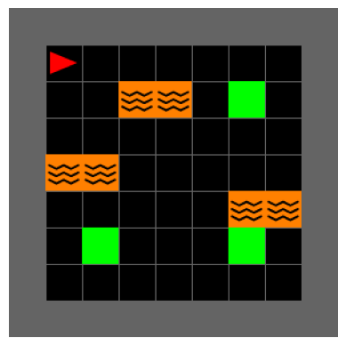
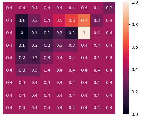
(a) 1st round

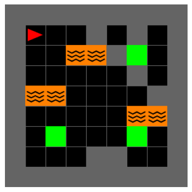
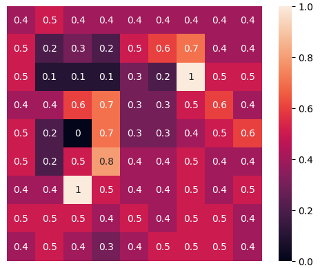
(b) 2nd round

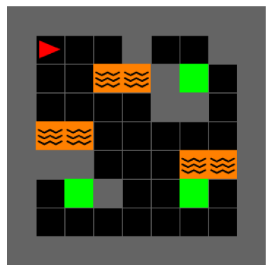
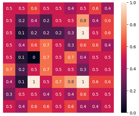
(c) 3rd round

Figure 1: The expert navigates to three possible goal states while avoiding lava in adaptively designed maze environments. For three consecutive rounds (a)-(c), we display the mazes constructed by ED-BIRL as well as the estimated reward functions after observing an expert trajectory in the current and past mazes. By adaptively designing environments and combining the expert demonstrations, we can recover the locations of goal states and lava states. In contrast, from observations in a fixed environment, e.g. repeatedly observing the expert in maze (a), it would be impossible to recover all relevant aspects of the reward function, i.e. goal states, as only the closest goal state will be visited by the expert (repeatedly). Observing the human expert’s actions in new and carefully constructed environments can thus lead to a more precise and robust estimate of the unknown reward function.

Outline.

After discussing related work in Section 2, we will formally establish our framework of Environment Design for Inverse Reinforcement Learning in Section 3. In Section 4 we then propose an environment design approach based on a minimax Bayesian regret objective and explain how to compute demo environments efficiently when the set of environments exhibits useful structure. Section 5 extends Bayesian IRL methods to the setting of learning from demonstrations in multiple environments. Finally, we perform a preliminary set of experiments in Section 6 with the goal of evaluating the benefits of carefully curating the set of demo environments for reward learning.

2 Related Work

(Active) IRL.

The goal of IRL [4, 5] is to find a reward function that explains observed behaviour, which is assumed to be approximately optimal. Two of the most popular approaches to the IRL problem are Bayesian IRL [11, 12, 13] and Maximum Entropy IRL [14, 15, 16]. In this work, we focus on extending the Bayesian IRL formulation to demonstrations in multiple environments as it provides a principled way to reason under reward uncertainty. This is also the typical IRL formulation under which Active IRL has been addressed in prior work.

In particular, the environment design problem that we consider can be viewed as one of active reward elicitation [17]. Prior work on active reward learning has focused on querying the expert for additional demonstrations in specific states [17, 18, 19], mainly with the goal of resolving the uncertainty that is due to the expert’s policy not being specified accurately in these states. In contrast, we consider the situation where we cannot directly query the expert for additional information in specific states, but instead sequentially choose demo environments for the expert to act in. Importantly, in our setting, the same state can be visited under different transition dynamics, which can be crucial to distinguish between two plausible reward functions. Hereto related, [20] consider a repeated IRL setting in which the learner can choose any task for the expert to complete (with full information of the expert policy). Recently, [21] also introduced Interactive IRL in which the learner interacts with a human in a collaborative Stackelberg game without knowledge of the joint reward function. This setting is similar to the framework presented here in that the leader in a Stackelberg game can be viewed as designing environments by committing to specific policies.

Environment Design for Reinforcement Learning.

Environment Design and Curriculum Learning for RL aim to design a sequence of environments with increasing difficulty to improve the training of an autonomous agent [22]. However, in contrast to our problem setup, observations in a generated training environments are cheap, as this only involves actions from an autonomous agent, not a human expert. As such, approaches like domain randomisation [23, 24] can be practical for RL, whereas they can be extremely inefficient and wasteful in an IRL setting. Moreover, in IRL we typically work with a handful of rounds only, so that slowly improving the environment generation process over thousands of training episodes (i.e. rounds) is impractical [25, 26]. Finally, we also have to deal with the additional challenge of not knowing the true reward function according to which the expert is going to act, which makes reliably predicting the expert’s behaviour in an environment difficult.

3 Problem Formulation

We now formally introduce the Environment Design for Inverse Reinforcement Learning framework. A Markov Decision Process (MDP) is a tuple $(\mathcal{S},\mathcal{A},T,\mathbf{R},\gamma,\omega)$, where $\mathcal{S}$ is a set of states, $\mathcal{A}$ is a set of actions, $T:\mathcal{S}\times\mathcal{A}\times\mathcal{S}\to[0,1]$ is a transition function, $\mathbf{R}:\mathcal{S}\to\mathbb{R}$ is a reward function, $\gamma$ a discount factor, and $\omega$ an initial state distribution. We assume that there is a set transition functions $\mathcal{T}$ from which $T$ can be selected. Similar models have been considered for the RL problem under the name of Underspecified MDPs [25] or Configurable MDPs [27, 28].

We assume that the true reward function, denoted $\mathbf{R}$, is unknown to the learner and consider the situation where the learning agent gets to interact with the human expert in a sequence of $m$ rounds. More precisely, every round $k\in[m]$, the learner gets to select a demo environment $T_{k}\in\mathcal{T}$ for which an expert trajectory $\tau_{k}$ is observed. Our objective is to adaptively select a sequence of demo environments $T_{1},\dots,T_{m}$ so as to recover a robust estimate of the unknown reward function. We describe the general framework for this interaction between learner and human expert in Algorithm 1. To summarise, a problem-instance in our setting is given by $(\mathcal{S},\mathcal{A},\mathcal{T},\mathbf{R},\gamma,\omega,m)$, where $\mathcal{T}$ is a set of environments, $\mathbf{R}$ is the unknown reward function, and $m$ the learner’s budget.

Algorithm 1 General Framework of Environment Design for Inverse Reinforcement Learning

1:  input  set of environments $\mathcal{T}$, resources $m\in\mathbb{N}$

2:  for k = 1, …, m do

3:     Choose an environment $T_{k}\in\mathcal{T}$                                 (Environment Design)

4:     Observe expert trajectory $\tau_{k}$ in environment $T_{k}$

5:     Estimate rewards from observations up to round $k$ (Inverse Reinforcement Learning)

From Algorithm 1 we see that the Environment Design for IRL problem has two main ingredients: a) choosing useful demo environments for the human to demonstrate the task in (Section 4), and b) inferring the reward function from expert demonstration in multiple environments (Section 5).

3.1 Preliminaries and Notation

Throughout the paper, note that $R$ denotes a generic reward function, whereas $\mathbf{R}$ refers to the true (unknown) reward function. We let $\mathcal{V}_{R,T}^{\pi}(s)\coloneqq\mathbb{E}[\sum_{t=0}^{\infty}\gamma^{t}R(s_{t})\mid\pi,T,s_{0}=s]$ denote the expected discounted return, i.e. value function, of a policy $\pi$ under some reward function $R$ and transition function $T$ in state $s$. For the value under the initial state distribution $\omega$, we then merely write ${\mathcal{V}_{R,T}^{\pi}\coloneqq\mathbb{E}_{s\sim\omega}[\mathcal{V}_{R,T}^{\pi}(s)]}$ and denote its maximum by $\mathcal{V}_{R,T}^{*}\coloneqq\max_{\pi}\mathcal{V}_{R,T}^{\pi}$. We accordingly refer to the ${Q}$-values under a policy $\pi$ by ${Q}_{R,T}^{\pi}(s,a)$ and their optimal values by ${Q}_{R,T}^{*}(s,a)$. In the following, we let $\pi_{R,T}$ always denote the optimal policy w.r.t. $R$ and $T$, i.e. the policy maximising the expected discounted return in the MDP $(\mathcal{S},\mathcal{A},T,R,\gamma,\omega)$.

We generally write $\tau$ for expert trajectories. In particular, these expert trajectories are always observed with respect to a specific transition function $T$. We therefore summarise the observation of an expert trajectory $\tau_{k}$ in an environment $T_{k}$ by $\mathcal{D}_{k}=(\tau_{k},T_{k})$ and write $\mathcal{D}_{1:k}=(\mathcal{D}_{1},\dots,\mathcal{D}_{k})$ for all observations up to (and including) the $k$-th round. We let $\mathbb{P}(\cdot\mid\mathcal{D}_{1:k})$ denote the posterior over reward functions given observations $\mathcal{D}_{1:k}$. For the prior $\mathbb{P}(\cdot)$, we introduce the convention that $\mathbb{P}(\cdot)=\mathbb{P}(\cdot\mid\mathcal{D}_{1:0})$. Out of convenience, we sometimes refer to transition functions $T$ as environments. In particular, when speaking of expert demonstrations in an environment $T$, we refer to expert demonstrations in the MDP $(\mathcal{S},\mathcal{A},T,\mathbf{R},\omega,\gamma)$, where $\mathbf{R}$ denotes the true (unknown) reward function that the expert is maximising.

4 Environment Design via Minimax Bayesian Regret

Our goal is to adaptively select demo environments for the expert based on our current belief about the reward function. We consider the situation where at round $k+1$ we have access to a posterior belief $\mathbb{P}(\cdot\mid\mathcal{D}_{1:k})$ over reward functions, which in practice can be approximated using a Bayesian IRL approach whose discussion we postpone to Section 5. In Section 4.1, we will introduce a minimax Bayesian regret objective for the environment design process which aims to select demo environments so as to ensure that our reward estimate is robust and risk-averse. Section 4.2 then deals with the computation of such environments when the set of demo environments exhibits a useful structure.

4.1 Minimax Bayesian Regret

We begin by reflecting on the potential loss of an agent when deploying a policy $\pi$ under transition function $T$ and the true reward function $\mathbf{R}$, given by the difference

$$\ell_{\mathbf{R}}(T,\pi)\coloneqq\mathcal{V}^{*}_{\mathbf{R},T}-\mathcal{V}_{\mathbf{R},T}^{\pi}.$$

The reward function $\mathbf{R}$ is unknown to us, so that we can instead use our belief $\mathbb{P}$ over reward functions and consider the Bayesian regret, i.e. loss, of a policy $\pi$ under $T$ and $\mathbb{P}$, i.e.

$$\operatorname{BR}_{\mathbb{P}}(T,\pi)\coloneqq\mathbb{E}_{R\sim\mathbb{P}}\big{[}\ell_{R}(T,\pi)\big{]}=\mathbb{E}_{R\sim\mathbb{P}}\big{[}\mathcal{V}^{*}_{R,T}-\mathcal{V}^{\pi}_{R,T}\big{]}.$$

The concept of Bayesian regret is well-known from, e.g.  online optimisation and online learning [29] and has been utilised for IRL in a slightly different form by [18]. The idea is that given a (prior) belief about some parameter, we evaluate our policy against an oracle that knows the true parameter. Typically, under such uncertainty about the true parameter (here, reward function) we are interested in risk-averse policies minimising the Bayesian regret, i.e.

$$\min_{\pi}\operatorname{BR}_{\mathbb{P}}(T,\pi).$$

To derive an objective for the environment design problem, we then consider a minimax game where one player selects the environment and the other the policy:

$$\max_{T\in\mathcal{T}}\min_{\pi\in\Pi}\operatorname{BR}_{\mathbb{P}}(T,\pi).$$ (1)

What this means is that we search for an environment $T\in\mathcal{T}$ such that the regret-minimising policy w.r.t. $\mathbb{P}$ suffers maximal regret against the optimal policies w.r.t. reward candidates $R\sim\mathbb{P}$. Note that this objective has the advantage of generally selecting environments that the expert can solve, as the regret in degenerate or purely adversarial environments will be close to zero. Moreover, the minimax Bayesian regret objective is performance-based and not purely uncertainty-based (such as prior objectives based on entropy, e.g. [17]). This is typically desired as reducing our uncertainty about the rewards in states that are not relevant under any transition function in $\mathcal{T}$ (e.g. states that are not being visited by any optimal policy) is unnecessary and generally a wasteful use of our budget. Finally, we also see that if the Bayesian regret objective becomes zero, the posterior mean is guaranteed to be optimal in every demonstration environment.

Lemma 1.

If for some posterior $\mathbb{P}(\cdot\mid\mathcal{D})$ it holds that $\max_{T\in\mathcal{T}}\min_{\pi\in\Pi}\operatorname{BR}_{\mathbb{P}}(T,\pi)=0$, then the posterior mean $\bar{R}=\mathbb{E}_{\mathbb{P}}[R]$ is optimal for every $T\in\mathcal{T}$, i.e. $\bar{R}$ induces an optimal policy in every environment in $\mathcal{T}$.

Algorithm 2 ED-BIRL: Environment Design for Bayesian IRL

1:  input  environments $\mathcal{T}$, prior distribution $\mathbb{P}$, resources $m\in\mathbb{N}$

2:  for $k=1,\dots,m$ do

3:     Sample rewards from $\mathbb{P}(\cdot\mid\mathcal{D}_{1:{k-1}})$ using $\texttt{BIRL}(\mathcal{D}_{1:k-1})$ (see Section 4.2)

4:     Construct empirical distribution ${\smash{\hat{\mathbb{P}}}}_{k-1}$ from sampled rewards

5:     Find $T_{k}\in\mathop{\rm arg\,max}_{T}\min_{\pi}\operatorname{BR}_{{\smash{\hat{\mathbb{P}}}}_{k-1}}(T,\pi)$ (see Section 5.1)

6:     Observe expert trajectory $\tau_{k}$ in $T_{k}$ and let $\mathcal{D}_{k}=(\tau_{k},T_{k})$

7:  return  $\texttt{BIRL}(\mathcal{D}_{1:m})$

In our algorithm ED-BIRL, we sample from the posterior to construct an empirical distribution for which we then find the maximin transition function (1). To sample from the posterior, we use an extension of Bayesian IRL methods to the case where we observe expert demonstrations in multiple environments as described in Section 5. The algorithm ED-BIRL is detailed in Algorithm 2. In the following, we will discuss how the maximin transition function $\mathop{\rm arg\,max}_{T}\min_{\pi}\operatorname{BR}_{\hat{\mathbb{P}}}(T,\pi)$ can be computed efficiently and consider the special case when the set of environments, $\mathcal{T}$, has a useful structure that we can exploit.

4.2 Environment Generation

Structured Environments.

Often the set of environments has a useful structure that can be used to search the space of environments $\mathcal{T}$ efficiently. We begin by recalling that the value function is linear in the rewards, so that we can rewrite equation (1) as

$$\max_{T}\min_{\pi}\operatorname{BR}_{\mathbb{P}}(T,\pi)=\max_{T}\big{\{}\mathbb{E}_{R\sim\mathbb{P}}[\mathcal{V}^{*}_{R,T}(s_{0}]-\max_{\pi}\mathcal{V}_{\bar{R},T}^{\pi}(s_{0})]\big{\}},$$

where $\bar{R}=\mathbb{E}_{R\sim\mathbb{P}}[R]$ is the mean of $\mathbb{P}$. We now consider the special case where each environment $T\in\mathcal{T}$ is build from a collection of transition matrices $T_{s}$.

Let $T_{s}\in\mathbb{R}^{\mathcal{S}\times A}$ denote a state-transition matrix dictating the transition probabilities in state $s$. Clearly, we can identify any transition function $T$ with a family of state-transition matrices $\{T_{s}\}_{s\in\mathcal{S}}$. We now say that an environment set $\mathcal{T}$ allows us to make state-individual transition choices if there exist sets $\mathcal{T}_{s}$ such that $\mathcal{T}=\{\{T_{s}\}_{s\in\mathcal{S}}\colon T_{s}\in\mathcal{T}_{s}\}$. In other words, we can construct a new environment $T$ by arbitrarily combining transition matrices for each state. Note that this of course allows for the case when the transitions in some state $s$ are fixed, i.e. we have the singleton $\mathcal{T}_{s}=\{T_{s}\}$. When we can make such state-individual transition choices, we can use an extended value iteration approach as detailed in Algorithm 3 that takes as input an empirical distribution ${\smash{\hat{\mathbb{P}}}}$ as in Line 4 in Algorithm 2.

Algorithm 3 Extended Value Iteration for Structured Environments

1:  input environments $\mathcal{T}=\{\mathcal{T}_{s}\}_{s\in\mathcal{S}}$, empirical distribution $\hat{\mathbb{P}}$ with mean $\bar{R}=\mathbb{E}_{R\sim\hat{\mathbb{P}}}[R]$

2:  repeat until $\mathcal{V}_{\bar{R}}$ and $\mathcal{V}_{R}$ converge:

3:  for $s\in\mathcal{S}$ do

4:     $T_{s}=\mathop{\rm arg\,max}\limits_{T_{s}\in\mathcal{T}_{s}}\Big{\{}\mathbb{E}_{R\sim\hat{\mathbb{P}}}\big{[}\max\limits_{a\in\mathcal{A}}T_{s,a}^{\top}\mathcal{V}_{R}\big{]}-\max\limits_{b\in\mathcal{A}}T_{s,b}^{\top}\mathcal{V}_{\bar{R}}\Big{\}}$

5:     $\mathcal{V}_{R}(s)=\max\limits_{a\in\mathcal{A}}R(s)+\gamma T_{s,a}^{\top}\mathcal{V}_{R}$ for every $R\sim\hat{\mathbb{P}}$

6:     $\mathcal{V}_{\bar{R}}(s)=\max\limits_{b\in\mathcal{A}}\bar{R}(s)+\gamma T_{s,b}^{\top}\mathcal{V}_{\bar{R}}$

7:  return  environment $T=\{T_{s}\}_{s\in\mathcal{S}}$

5 Inverse Reinforcement Learning with Multiple Environments

We now analyse how we can learn about the reward function from demonstrations that were provided under multiple, different environment dynamics. Recall that we consider the situation where the learner observes expert trajectories with respect to the same reward function under possibly different transition dynamics. In the following, we explain how to extend Bayesian IRL methods to this setting.

5.1 Bayesian IRL

The Bayesian perspective to the IRL problem provides a principled way to reason about reward uncertainty [11]. Typically, the human is modelled by a Boltzmann-rational policy [30]. This means that for a given reward function $R$ and transition function $T$ the expert is acting according to a policy

$$\pi^{\textrm{softmax}}_{R,T}(a\mid s)=\frac{\exp(c{Q}^{*}_{R,T}(s,a))}{\sum_{a^{\prime}}\exp(c{Q}^{*}_{R,T}(s,a^{\prime}))},$$ (2)

where the parameter $c$ relates to our judgement of the expert’s optimality. Given a prior distribution $\mathbb{P}(\cdot)$, the goal of Bayesian IRL is to recover the posterior distribution $\mathbb{P}(\cdot\mid\mathcal{D})$ and to either sample from the posterior using MCMC [11, 12] or perform MAP estimation [13]. In our case, the data is given by the sequence $\mathcal{D}_{1:k}=(\mathcal{D}_{1},\dots,\mathcal{D}_{k})$ with $\mathcal{D}_{k}=(\tau_{k},T_{k})$. We see that this is no obstacle as the likelihood factorises as

$$\mathbb{P}(\mathcal{D}_{1:k}\mid R)=\prod_{i\leq k}\mathbb{P}(\tau_{i}\mid R,T_{i}),$$

since the expert trajectories (i.e. expert policies) are conditionally independent given the reward function and transition function. The likelihood of each expert demonstration is then given by $\smash{\mathbb{P}(\tau_{i}\mid R,T_{i})=\prod_{(s,a)\in\tau_{i}}\pi^{\textrm{softmax}}_{R,T_{i}}(a\mid s)}$, where $\pi^{\textrm{softmax}}_{R,T_{i}}$ is the Boltzmann-rational policy as defined in (2). As a result, we can, for instance, sample from the posterior using the Policy-Walk algorithm from [11] with minor modifications or the Metropolis-Hastings Simplex-Walk algorithm from [21]. Other Bayesian approaches, e.g. those that model the reward function as a Gaussian process [31] or take a variational inference approach [32], can similarly be adapted to demonstrations from multiple environments by using the factorisation of the likelihood. We generally denote any Bayesian IRL algorithm that is capable of sampling from the posterior by BIRL.

6 Experiments

We perform a preliminary set of experiments on a maze task as well as randomly generated MDPs. Our primary goal is to address the following two questions:

1. Can we recover the true reward function by adaptively designing demo environments?

2. Can we learn more robust reward functions by adaptively designing demo environments?

6.1 Recovering the True Reward Function

In this experiment, we consider a maze task in which the learner has the ability to add obstacles to a base layout of the maze. We visualise the designed mazes and estimated rewards and evaluate whether our approach can recover the true reward function by adaptively constructing these mazes.

Experimental Setup.

We consider a maze task in which the goal is to reach one of three goal states while avoiding lava. Here, the learner is able to add obstacles to cells and observes two expert trajectories for each constructed maze, which is done to give a stronger learning signal to BIRL so as to require fewer samples. The true reward function, which is unknown to the learner, yields reward $1$ in goal states and reward $-1$ in lava states. We consider two different base layouts: a basic layout with goal states and lava evenly spread out, Figure 2 (a)-(c), and a second layout with vertical strips of lava which make it challenging to construct mazes so that the right side of the world is being visited, Figure 2 (d)-(f). We compare our approach, ED-BIRL, with learning from a fixed maze, and learning from mazes that were randomly created. We randomly generate these mazes by adding an obstacle to a cell with probability $0.3$. The inference for all three approaches is done using BIRL and the computed reward estimates are scaled to $[0,1]$ and rounded.

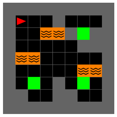
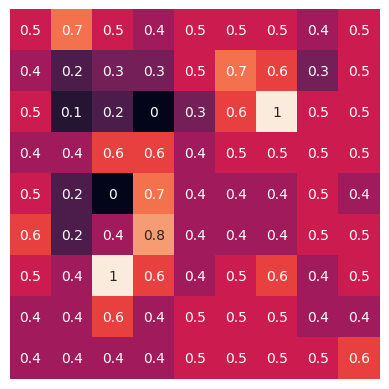
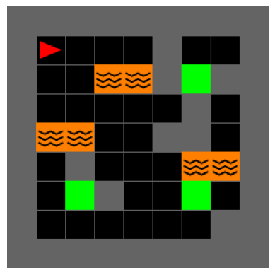
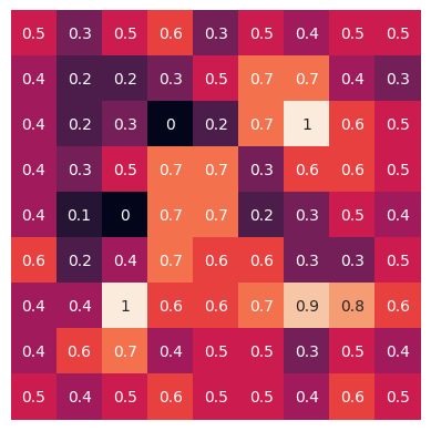
(a) ED-BIRL

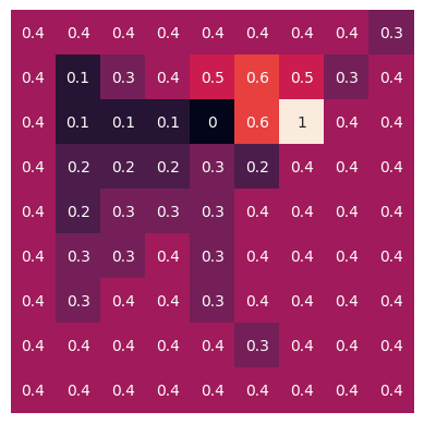
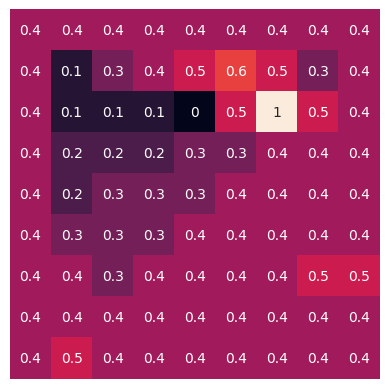
(b) Fixed Environment IRL

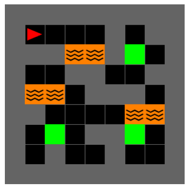
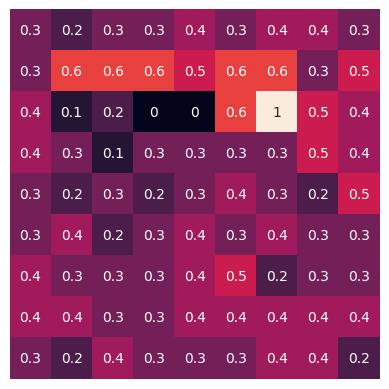
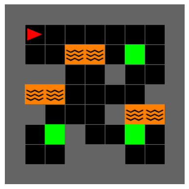
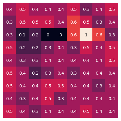
(c) Domain Randomisation

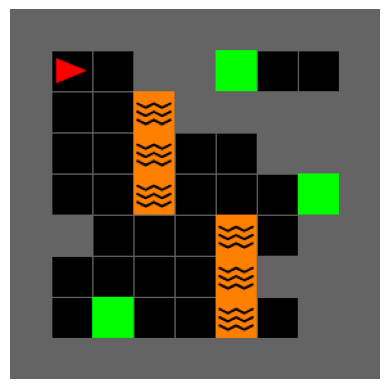
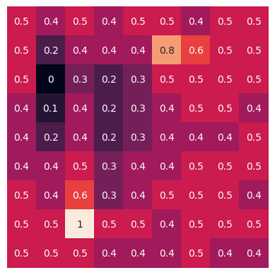
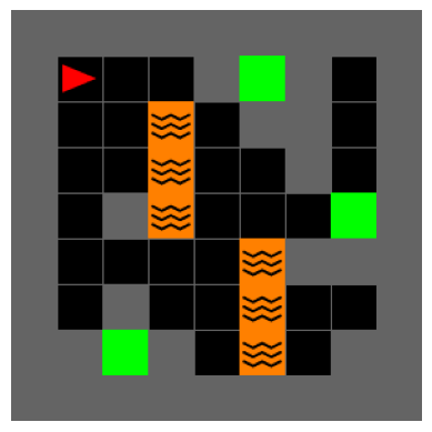
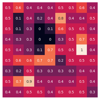
(d) ED-BIRL

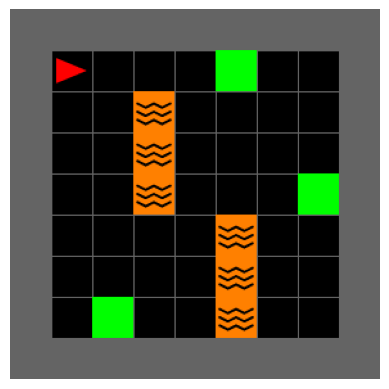
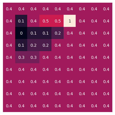
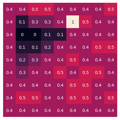
(e) Fixed Environment IRL

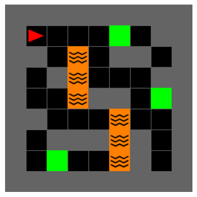
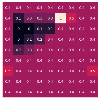
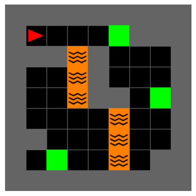
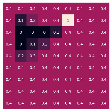
(f) Domain Randomisation

Figure 2: Comparison of ED-BIRL, Fixed Environment IRL, and Domain Randomisation for two versions of the maze problem: (a)-(c) and (d)-(f). In each case, we display three consecutive rounds and the corresponding mazes and estimated rewards. We use the same colour scale as in Figure 1, which ranges from black (0.0) to red (0.5) to white (1.0).

Results.

In Figure 2, we observe that ED-BIRL recovers the location of all three goal states after three rounds in both maze layouts. Moreover, the learner is able to identify the location of all lava strips in Figure 2(a), i.e. states with negative reward. In Figure 2(d), ED-BIRL also recovered the rewards of the upper lava region, whereas the estimates for the lower lava region are more imprecise (while they are also less performance-relevant). By adaptively designing a sequence of demo environments, ED-BIRL is thus capable of recovering (all performance-relevant aspects of) the unknown reward function.

In contrast, learning from a fixed environment (Figure 2(b), 2(e)) as well as domain randomisation (Figure 2(c), 2(f)) fail to recover the location of all goal states, let alone lava. In a fixed maze, any near-optimal policy will visit the closest goal state only, which in this case is the top right corner in both versions of the maze. We also see that using domain randomisation is impractical for IRL, as we require carefully constructed mazes to recover the true reward function. Even worse, by obliviously randomising the maze layout, we may create unsolvable environments for the human expert, which yield no information at all (see e.g. Figure 2(c)).

6.2 Learning Robust Reward Functions

In this experiment, we provide the learner with a set of demo environments they can select for a demonstration. Afterwards, the agent is evaluated on a set of test environments. The performance in the test set captures the generalisation ability of the learned rewards to new dynamics.

Experimental Setup.

We first randomly generate a base MDP $(\mathcal{S},\mathcal{A},{T_{\texttt{base}}},\mathbf{R},\gamma,\omega)$ with base transition function ${T_{\texttt{base}}}$. We then construct the set of possible demo environments, here denoted $\mathcal{T}_{\texttt{demo}}$ instead of $\mathcal{T}$ to clearly distinguish between demo and test environments, by sampling state-transition functions that differ from the base transitions ${T_{\texttt{base}}}$ by at most some value $\rho_{\texttt{demo}}$ in terms of $\ell_{\infty}$-distance. In our experiments, we set the maximum amount of variation in the demo environments to $\rho_{\texttt{demo}}=0.5$. Similarly, we create a set of test environments $\mathcal{T}_{\texttt{test}}$ with a maximum amount of perturbation $\rho_{\texttt{test}}$ on which we evaluate the learned reward functions. For all three approaches, we evaluate the posterior mean, which is computed using BIRL. For all $T\in\mathcal{T}_{\texttt{test}}$, we optimise a policy w.r.t. the posterior mean and $T$ and evaluate the computed policy under the true reward function $\mathbf{R}$ and transition function $T$. Finally, we average the results over all environments in $\mathcal{T}_{\texttt{test}}$. We want to emphasise that the way we construct $\mathcal{T}_{\texttt{demo}}$ and $\mathcal{T}_{\texttt{test}}$, these sets are completely disjunct except for the base transition function, i.e. $\mathcal{T}_{\texttt{demo}}\cap\mathcal{T}_{\texttt{test}}=\{{T_{\texttt{base}}}\}$. We therefore do not observe the expert in the environments that we evaluate our approaches on.

Results.

In Figure 3(a), we observe that ED-BIRL outperforms domain randomisation and learning from a fixed environments over the course of all rounds. As expected, the loss of all three approaches increases the more diverse the test environments are and the more they differ from the base environment, which can be seen in Figure 3(b). Interestingly, even for $\rho_{\texttt{test}}=0$, i.e. evaluation on the base environment only, ED-BIRL slightly outperforms learning directly from the fixed base environment suggesting a superior sample-efficiency of ED-BIRL.

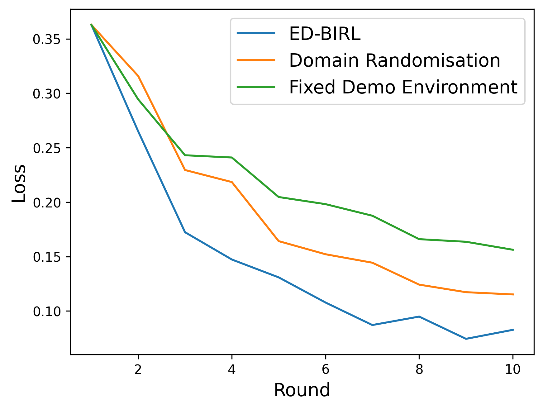
(a) Average utility loss of ED-BIRL, Domain Randomisation, and Fixed Environment IRL over $10$ rounds. The learned rewards are evaluated on a set of test environments that differ from the base environment by at most $\rho_{\texttt{test}}=0.5$.

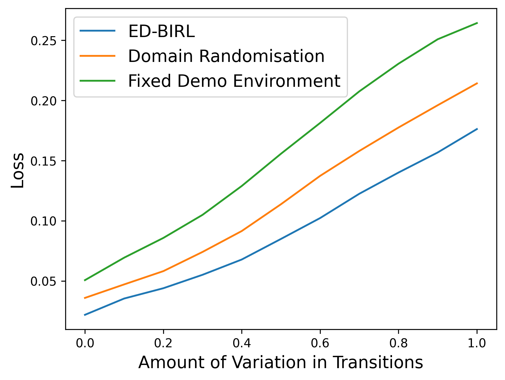
(b) Along the $x$-axis we increase $\rho_{\texttt{test}}$, i.e. the amount of variation in the test environments. We evaluate the learned reward functions after $10$ rounds of interaction with the expert, i.e. the final reward estimate from Figure 3(a).

Figure 3: On a randomly generated MDP task, we evaluate the robustness of reward estimates learned by ED-BIRL, Domain Randomisation, and Fixed Environment IRL, respectively.

7 Discussion

The presented work gives a first glance into Environment Design for Inverse Reinforcement Learning. In this paper, we focus on the Bayesian setting, where a belief about the reward function is computed using Bayesian IRL (with observations from multiple environments). This allowed us to reason about reward uncertainty in a principled way, guiding our environment design approach via a minimax Bayesian regret objective. A future version of this work will consider non-Bayesian IRL frameworks and explain how to perform environment design with point estimates of the reward function (instead of Bayesian beliefs). In future work it will also be interesting to consider a batch version of this setting, where the learner has to decide on a batch of demo environments every round.

Appendix A Appendix

A.1 Proofs

Proof of Lemma 1.

For simplicity of exposition, we assume here that the posterior $\mathbb{P}$ is discrete. Now, as the value function is linear in rewards, we have

$$\min_{\pi}\operatorname{BR}_{\mathbb{P}}(T,\pi)=\operatorname{BR}_{\mathbb{P}}(T,\pi_{\bar{R},T}),$$

where $\pi_{\bar{R},T}$ is the optimal policy w.r.t. the posterior mean $\bar{R}=\mathbb{E}_{R\sim\mathbb{P}}[R]$ and the transition function $T$. If $\max_{T\in\mathcal{T}}\min_{\pi\in\Pi}\operatorname{BR}_{\mathbb{P}}(T,\pi)=0$, it then follows that $\max_{T\in\mathcal{T}}\operatorname{BR}_{\mathbb{P}}(T,\pi_{\bar{R},T})=0$, i.e. $\mathcal{V}_{R,T}^{*}=\mathcal{V}_{R,T}^{\pi_{\bar{R},T}}$ for all $R\in\mathop{\rm supp}(\mathbb{P})$ and $T\in\mathcal{T}$. This must imply that $\mathcal{V}_{\mathbf{R},T}^{*}=\mathcal{V}_{\mathbf{R},T}^{\pi_{\bar{R},T}}$ for all $T\in\mathcal{T}$. In other words, $\bar{R}$ is optimal for all $T\in\mathcal{T}$ (under the initial state distribution $\omega$). ∎

A.2 More Experimental Details

The BIRL method we used for the experiments is a straightforward extension of Algorithm 1 in [12] to multiple environments following our explanations in Section 5.1.

Recovering the True Reward Function.

For the experiments in Section 6.1, we let the learner observe two trajectories for each maze. This was done in order to speed up the inference of BIRL and reduce the computational cost. The expert was modeled by a Boltzmann-rational policy and thus uniformly selected an optimal action when there were several optimal ones in a given state.

Learning Robust Reward Functions.

For the experiments in Section 6.2, we randomly generated an MDP with 50 states and 4 actions using a Dirichlet distribution for the transitions and a Beta distribution for the reward function. For each state we let the demo set of environments contain 15 choices. The size of the test environments was set to be $|\mathcal{T}_{\texttt{test}}|=500$. Every round, the learner got to select a demo environment and observe a single expert trajectory in that environment. We limited the amount of deviation from the base transitions in our experiments according to $\rho_{\texttt{demo}}$ and $\rho_{\texttt{test}}$. In particular, note that any choice of $\rho_{\texttt{demo}}$ implies that $\lVert{T_{\texttt{base}}}-T\rVert_{\infty}=\max_{s,a}\lVert{T_{\texttt{base}}}(\cdot\mid s,a)-T(\cdot\mid s,a)\rVert_{1}\leq\rho_{\texttt{demo}}$ for all $T\in\mathcal{T}_{\texttt{demo}}$. The results were averaged over $5$ complete runs, i.e. for $5$ randomly generated problem instances.

A.3 Environment Design with Arbitrary Environments

In some situations, the set of demo environments $\mathcal{T}$ may not exhibit any useful structure. Moreover, we may not even have explicit knowledge of the transition functions in $\mathcal{T}$, but can only access a set of corresponding simulators. In this case, we are left with approximating the maximin environment (1) by sampling simulators from $\mathcal{T}$ and performing policy rollouts (see Algorithm 4).

Algorithm 4 Environment Design with Arbitrary Environments

1:  input  set of environments $\mathcal{T}$, rewards $\{R_{1},\dots,R_{k}\}$, best guess $\bar{R}$

2:  // if necessary, sample a subset $\mathcal{T}_{\subset}$ from $\mathcal{T}$

3:  for $T\in\mathcal{T}$ do

4:     calculate $\pi^{*}=\pi^{*}_{\bar{\bar{R}},T}$ (policy optimisation)

5:     for $R\in\{R_{1},\dots,R_{k}\}$ do

6:        evaluate $\mathcal{V}_{R,T}^{\pi^{*}}$ (policy evaluation)   

7:        calculate $\mathcal{V}_{R,T}^{*}=\max_{\pi}\mathcal{V}_{R,T}^{\pi}$ (policy optimisation)

8:        $\ell(R)=\max_{\pi}\mathcal{V}_{R,T}^{*}-\mathcal{V}_{R,T}^{\smash{\pi^{*}}}$

9:     $\operatorname{BR}(T)=\sum_{R\in\{R_{1},\dots,R_{k}\}}\ell(R)$

10:  return  $T^{*}=\mathop{\rm arg\,max}_{T\in\mathcal{T}}\operatorname{BR}(T)$

A.4 Maximum Entropy IRL with Multiple Environments

In the following, we give a brief outline of how Maximum Entropy (MaxEnt) IRL methods can be extended to multiple environments. For a practical algorithm we choose to extend the popular Adversarial IRL algorithm [7].

In MaxEnt IRL, the reward function is assumed to be parameterised by some vector $\theta$. While some work has considered non-linear parameterisation of the reward function, e.g. [16], we can generally think of the reward function being linear in some feature vector $\mathbf{f}$, i.e. $R_{\theta}(s)=\theta^{\top}\mathbf{f}_{s}$. Under the MaxEnt model, the probability of trajectories is exponentially dependent on their value:

$$\mathbb{P}(\tau\mid\theta,T)=\frac{e^{R_{\theta}(\tau)}}{Z(\theta,T)}\prod_{t=1}^{|\tau|}T(s_{t+1}\mid s_{t},a_{t}),$$ (3)

where $Z(\theta,T)$ is the partition function given by

$$Z(\theta,T)=\sum_{\tau}e^{R_{\theta}(\tau)}\prod_{t=1}^{|\tau|}T(s_{t+1}\mid s_{t},a_{t}).$$ (4)

Note that here the sum over $\tau$ is over all possible trajectories. Our goal is then to solve the maximum likelihood problem

$$\mathop{\rm arg\,max}_{\theta}\sum_{(\tau,T)\in\mathcal{D}}\log\mathbb{P}(\tau\mid\theta,T).$$ (5)

We see that the only difference to the original MaxEnt IRL formulation is that we now sum over pairs $(\tau,T)$ instead of just $\tau$. As a scalable solution to the MaxEnt IRL problem, Adversarial IRL [7] as well as GAIL [15, 33] cast the optimisation of (5) as a generative adversarial network (with different discriminators). To extend Adversarial IRL, we consider a set of policies $\pi_{1},\dots,\pi_{k}$, used to generate trajectories in environments $T_{1},\dots,T_{k}$, and discriminators $D_{1,\theta,\phi},\dots D_{k,\theta,\phi}$ given by

$$D_{i,\theta,\phi}(s,a,s^{\prime})=\frac{\exp(f_{\theta,\phi}(s,a,s^{\prime}))}{\exp(f_{\theta,\phi}(s,a,s^{\prime}))+\pi_{i}(a\mid s)}$$ (6)

with

$$f_{\theta,\phi}(s,a,s^{\prime})=g_{\theta}(s)+\gamma h_{\phi}(s^{\prime})-h_{\phi}(s),$$ (7)

where $g_{\theta}(s)$ is the reward approximator and $h_{\phi}$ a shaping term (see [7]).

Algorithm 5 Adversarial IRL with Multiple Environments

1:  input  Observations $\mathcal{D}=(\mathcal{D}_{1},\dots,\mathcal{D}_{k})$ with $\mathcal{D}_{i}=(\tau_{i},T_{i})$

2:  Initialise policies $\pi_{1},\dots,\pi_{k}$ and discriminators $D_{1,\theta,\phi},\dots,D_{k,\theta,\phi}$

3:  for $t=0,1,\dots$ do

4:     Collect trajectories $\tau^{G}_{i,j}=(s_{0},a_{0},\dots,s_{H},a_{H})$ by executing $\pi_{i}$ in $T_{k}$ for $i\in[k]$.

5:     Train discriminators $D_{1,\theta,\phi}\dots,D_{k,\theta,\phi}$ to classify expert data $\tau_{1},\dots,\tau_{k}$ from samples $\{\tau^{G}_{1,j}\}_{j},\dots,\{\tau^{G}_{k,j}\}_{j}$, respectively, via logistic regression with shared parameter $\theta$.

6:     Update reward $R_{\theta,\phi}(s,a,s^{\prime})\leftarrow\sum_{i=1}^{k}\Big{(}\log D_{i,\theta,\phi}(s,a,s^{\prime})-\log(1-D_{i,\theta,\phi}(s,a,s^{\prime}))\Big{)}$.

7:     Update $\pi_{1},\dots,\pi_{k}$ with respect to $R_{\theta,\phi}$ using any policy optimisation method.

With minor modifications, a justification of Algorithm 5 can be done analogous to that in [7].

References

- Mnih et al. [2015] Volodymyr Mnih, Koray Kavukcuoglu, David Silver, Andrei A Rusu, Joel Veness, Marc G Bellemare, Alex Graves, Martin Riedmiller, Andreas K Fidjeland, Georg Ostrovski, et al. Human-level control through deep reinforcement learning. nature, 518(7540):529–533, 2015.
- Lillicrap et al. [2015] Timothy P Lillicrap, Jonathan J Hunt, Alexander Pritzel, Nicolas Heess, Tom Erez, Yuval Tassa, David Silver, and Daan Wierstra. Continuous control with deep reinforcement learning. arXiv preprint arXiv:1509.02971, 2015.
- Levine et al. [2016] Sergey Levine, Chelsea Finn, Trevor Darrell, and Pieter Abbeel. End-to-end training of deep visuomotor policies. The Journal of Machine Learning Research, 17(1):1334–1373, 2016.
- Russell [1998] Stuart Russell. Learning agents for uncertain environments. In Proceedings of the eleventh annual conference on computational learning theory, pages 101–103, 1998.
- Ng and Russell [2000] Andrew Y. Ng and Stuart J. Russell. Algorithms for inverse reinforcement learning. In Proceedings of the Seventeenth International Conference on Machine Learning, page 2, 2000.
- Arora and Doshi [2021] Saurabh Arora and Prashant Doshi. A survey of inverse reinforcement learning: Challenges, methods and progress. Artificial Intelligence, 297:103500, 2021.
- Fu et al. [2018] Justin Fu, Katie Luo, and Sergey Levine. Learning robust rewards with adverserial inverse reinforcement learning. In International Conference on Learning Representations, 2018. URL https://openreview.net/forum?id=rkHywl-A-.
- Toyer et al. [2020] Sam Toyer, Rohin Shah, Andrew Critch, and Stuart Russell. The magical benchmark for robust imitation. Advances in Neural Information Processing Systems, 33:18284–18295, 2020.
- Cao et al. [2021] Haoyang Cao, Samuel Cohen, and Lukasz Szpruch. Identifiability in inverse reinforcement learning. Advances in Neural Information Processing Systems, 34:12362–12373, 2021.
- Kim et al. [2021] Kuno Kim, Shivam Garg, Kirankumar Shiragur, and Stefano Ermon. Reward identification in inverse reinforcement learning. In International Conference on Machine Learning, pages 5496–5505. PMLR, 2021.
- Ramachandran and Amir [2007] Deepak Ramachandran and Eyal Amir. Bayesian inverse reinforcement learning. In Proceedings of the 20th International Joint Conference on Artifical Intelligence, pages 2586–2591, 2007.
- Rothkopf and Dimitrakakis [2011] Constantin A Rothkopf and Christos Dimitrakakis. Preference elicitation and inverse reinforcement learning. In Joint European conference on machine learning and knowledge discovery in databases, pages 34–48, 2011.
- Choi and Kim [2011] Jaedeug Choi and Kee-eung Kim. Map inference for bayesian inverse reinforcement learning. In Advances in Neural Information Processing Systems, volume 24. Curran Associates, Inc., 2011. URL https://proceedings.neurips.cc/paper/2011/file/3a15c7d0bbe60300a39f76f8a5ba6896-Paper.pdf.
- Ziebart et al. [2008] Brian D Ziebart, Andrew L Maas, J Andrew Bagnell, Anind K Dey, et al. Maximum entropy inverse reinforcement learning. In Aaai, volume 8, pages 1433–1438. Chicago, IL, USA, 2008.
- Ho and Ermon [2016] Jonathan Ho and Stefano Ermon. Generative adversarial imitation learning. Advances in neural information processing systems, 29, 2016.
- Finn et al. [2016a] Chelsea Finn, Sergey Levine, and Pieter Abbeel. Guided cost learning: Deep inverse optimal control via policy optimization. In International conference on machine learning, pages 49–58. PMLR, 2016a.
- Lopes et al. [2009] Manuel Lopes, Francisco Melo, and Luis Montesano. Active learning for reward estimation in inverse reinforcement learning. In Joint European Conference on Machine Learning and Knowledge Discovery in Databases, pages 31–46. Springer, 2009.
- Brown et al. [2018] Daniel S Brown, Yuchen Cui, and Scott Niekum. Risk-aware active inverse reinforcement learning. In Conference on Robot Learning, pages 362–372. PMLR, 2018.
- Lindner et al. [2021] David Lindner, Matteo Turchetta, Sebastian Tschiatschek, Kamil Ciosek, and Andreas Krause. Information directed reward learning for reinforcement learning. Advances in Neural Information Processing Systems, 34:3850–3862, 2021.
- Amin et al. [2017] Kareem Amin, Nan Jiang, and Satinder Singh. Repeated inverse reinforcement learning. Advances in neural information processing systems, 30, 2017.
- Büning et al. [2022] Thomas Kleine Büning, Anne-Marie George, and Christos Dimitrakakis. Interactive inverse reinforcement learning for cooperative games. In International Conference on Machine Learning, pages 2393–2413. PMLR, 2022.
- Narvekar et al. [2020] Sanmit Narvekar, Bei Peng, Matteo Leonetti, Jivko Sinapov, Matthew E Taylor, and Peter Stone. Curriculum learning for reinforcement learning domains: A framework and survey. arXiv preprint arXiv:2003.04960, 2020.
- Tobin et al. [2017] Josh Tobin, Rachel Fong, Alex Ray, Jonas Schneider, Wojciech Zaremba, and Pieter Abbeel. Domain randomization for transferring deep neural networks from simulation to the real world. In 2017 IEEE/RSJ international conference on intelligent robots and systems (IROS), pages 23–30. IEEE, 2017.
- Akkaya et al. [2019] Ilge Akkaya, Marcin Andrychowicz, Maciek Chociej, Mateusz Litwin, Bob McGrew, Arthur Petron, Alex Paino, Matthias Plappert, Glenn Powell, Raphael Ribas, et al. Solving rubik’s cube with a robot hand. arXiv preprint arXiv:1910.07113, 2019.
- Dennis et al. [2020] Michael Dennis, Natasha Jaques, Eugene Vinitsky, Alexandre Bayen, Stuart Russell, Andrew Critch, and Sergey Levine. Emergent complexity and zero-shot transfer via unsupervised environment design. Advances in Neural Information Processing Systems, 33:13049–13061, 2020.
- Gur et al. [2021] Izzeddin Gur, Natasha Jaques, Yingjie Miao, Jongwook Choi, Manoj Tiwari, Honglak Lee, and Aleksandra Faust. Environment generation for zero-shot compositional reinforcement learning. Advances in Neural Information Processing Systems, 34:4157–4169, 2021.
- Metelli et al. [2018] Alberto Maria Metelli, Mirco Mutti, and Marcello Restelli. Configurable markov decision processes. In International Conference on Machine Learning, pages 3491–3500. PMLR, 2018.
- Ramponi et al. [2021] Giorgia Ramponi, Alberto Maria Metelli, Alessandro Concetti, and Marcello Restelli. Learning in non-cooperative configurable markov decision processes. Advances in Neural Information Processing Systems, 34, 2021.
- Russo and Van Roy [2014] Daniel Russo and Benjamin Van Roy. Learning to optimize via information-directed sampling. Advances in Neural Information Processing Systems, 27, 2014.
- Jeon et al. [2020] Hong Jun Jeon, Smitha Milli, and Anca Dragan. Reward-rational (implicit) choice: A unifying formalism for reward learning. Advances in Neural Information Processing Systems, 33:4415–4426, 2020.
- Levine et al. [2011] Sergey Levine, Zoran Popovic, and Vladlen Koltun. Nonlinear inverse reinforcement learning with gaussian processes. Advances in neural information processing systems, 24, 2011.
- Chan and van der Schaar [2021] Alex James Chan and Mihaela van der Schaar. Scalable Bayesian inverse reinforcement learning. In International Conference on Learning Representations, 2021. URL https://openreview.net/forum?id=4qR3coiNaIv.
- Finn et al. [2016b] Chelsea Finn, Paul Christiano, Pieter Abbeel, and Sergey Levine. A connection between generative adversarial networks, inverse reinforcement learning, and energy-based models. arXiv preprint arXiv:1611.03852, 2016b.