The Luminosity Function of Tidal Disruption Flares for the ZTF-I Survey

Abstract

The high-cadence survey of Zwicky Transient Facility (ZTF) has completely dominated the discovery of tidal disruption events (TDEs) in the past few years and resulted in the largest sample of TDEs with optical/UV light curves well-sampled around their peaks, providing us an excellent opportunity to construct a peak luminosity function (LF) of tidal disruption flares (TDFs). The new construction is necessary particularly considering that the most updated LF reported in literature has been inferred from only 13 sources from 5 different surveys. Here we present the optical and blackbody LFs calculated by 33 TDFs discovered in the ZTF-I survey. The optical LF can be described by both a power-law profile $dN/dL_{g}\propto L_{g}^{-2.3\pm 0.2}$, and a Schechter-like function. The blackbody LF can be described by a power-law profile $dN/dL_{\rm bb}\propto L_{\rm bb}^{-2.2\pm 0.2}$, shallower than the LF made of previous van Velzen (2018) sample. A possible low-luminosity turnover in the optical LF supports an Eddington-limited emission scenario. The drop of volumetric rate at high luminosity suggests a rate suppression due to direct captures of the black hole. The total volumetric rate is one order of magnitude lower than the previous estimation, which is probably not simply caused by the high fraction post-peak sources (7/13) in the previous sample. Instead, the normalization step during the previous LF construction to reconcile various surveys might adversely amplify the influence of serendipitous discoveries. Therefore, TDFs selected from ongoing and upcoming uniform surveys like ZTF, Vera Rubin Observatory (VRO) and Wide-Field Survey Telescope (WFST) should yield more accurate LFs.

1 Introduction

A tidal disruption event (TDE) happens when a massive black hole (BH) in the galaxy center tears apart an unlucky star that wanders too close, as the tidal forces overcome the self-gravity of the star. About half of the stellar debris will circularize and be accreted by the BH, producing a luminous flare that peaks from ultraviolet (UV) to soft X-ray band (e.g., Rees, 1988; Gezari, 2021). The occurrence rate of TDEs is about $10^{-4}-10^{-5}$ galaxy^-1 year^-1 (e.g., Wang & Merritt, 2004; Stone & Metzger, 2016). Although the first TDE was discovered in the X-ray band (Bade et al., 1996), the optical bands have dominated the discovery of TDEs in the past decade, thanks to the large survey area and the high cadence of the time-domain surveys, such as All-Sky Automated Survey for Supernovae (ASAS-SN, Shappee et al., 2014) and the Zwicky Transient Facility (ZTF, Bellm et al., 2019a). The total number of TDEs is now increasing at the rate of $\sim 10-20$ per year, and is predicted to skyrocket at the pace of a few thousand per year, as the larger surveys by Vera Rubin Observatory (VRO, Ivezić et al., 2019) and the Wide-Field Survey Telescope (WFST) are both scheduled to begin in 2023 (e.g., Strubbe & Quataert, 2009; van Velzen et al., 2011; Thorp et al., 2019; Bricman & Gomboc, 2020; Roth et al., 2021; Lin et al., 2022).

Tidal disruption flares (TDFs) in optical bands are mainly characterized by three features. First, the spectral energy distribution (SED) can be well described by a blackbody component, with the temperature varies slowly between $(1-5)\times 10^{4}$ K. This results in the steady blue color in optical bands (e.g. $g-r<0$). Second, the optical light curve of a TDF usually shows a monthly rise to a peak blackbody luminosity of $L_{\rm{bb}}\sim 10^{43-45}$ erg s^-1, followed by a power-law like decline that lasts for months to years. Third, the broad H$\alpha$, H$\beta$ or He ii emission lines usually appear in the spectra of TDFs near the peak, and then gradually narrow and weaken as the luminosity declines. Nonetheless, emission line features in some TDFs are too intense to distinguished, as a strong blue continuum dominates their spectra. These features are extracted from previous serendipitous discoveries, and now they instruct the search of TDFs for some large transient surveys. Most outstandingly, the ZTF-I survey has discovered around 30 TDFs, which consists the largest systematical sample of TDFs (Hammerstein et al., 2022).

In spite of a persistent number increase and gradually improved characterization of optical TDEs, their real event rate and emission origin remain rather uncertain (e.g., Piran et al., 2015; Jiang et al., 2016; Metzger & Stone, 2016; Dai et al., 2018; Lu & Bonnerot, 2020). The TDE event rate can indicate the stellar dynamics in galaxy centers, which determines how stars are fed to the loss cone (e.g., Merritt & Poon, 2004; Stone et al., 2020). Earlier rough TDE rate estimation based on very few luminous events, such as the two in SDSS (van Velzen & Farrar, 2014) and the other two in ASAS-SN survey (Holoien et al., 2016), resulted in a significantly lower rate than theoretical expectation albeit with large uncertainties. A well-constrained luminosity function (LF) extended to faint end can definitely help make progress on the measurement. Meanwhile, the LF might also shed useful insight into the physical process following the disruption and the correlation between optically and X-ray bright TDEs from a statistical point of view.

However, the most updated LF of optical/UV TDF remains the one proposed by van Velzen (2018), which is constructed with a sample of 13 sources, that is almost all optical/UV TDFs up to then. It is worthwhile to note that 7 out of 13 sources have only post-peak light curves, indicating a possible underestimate of peak luminosity. As a result, the maximum redshift ($z_{\rm{max}}$) for detection and identification of these sources might be underestimated and the volumetric rate of TDFs is thus overestimated. In addition, these TDFs are discovered by 5 surveys ($GALEX$, SDSS, PS1, iPTF, ASAS-SN) with different survey areas, depths, filters and cadences. Therefore, a normalization based on the TDF number in each survey has to be applied. This may amplify the influence for some serendipitous searches. In contrast, the TDF sample given by ZTF-I survey has several obvious advantages. First, it is $\sim 2.5$ times larger than the previous sample. Second, almost all TDFs are captured before or around their peaks, allowing a reliable measurement of their peak luminosity. Third, the TDFs are systematically selected by a single detector, precluding the serendipity. Last but not least, most TDFs are also followed by $Swift$ UVOT in the UV bands, which is very useful to constrain their blackbody temperature, radius and luminosity. In a word, it is meaningful to reconstruct a LF using the TDF sample of ZTF-I survey.

The outline of the paper is as follows. We will first introduce the TDF sample of ZTF-I survey, the follow-up observations of $Swift$ UVOT and the additional photometric data in Section 2. Next, in Section 3, we will describe the method of fitting to a blackbody model, and show the fitting results. We will construct the LF in Section 4, then briefly discuss the results in Section 5. Finally, we conclude in Section 6. We adopt a flat cosmology with $H_{0}=70$ km s^-1 Mpc^-1 and $\Omega_{\Lambda}=0.7$. All magnitudes are in the AB (Oke, 1974) system.

1.1 TDE or TDF

In the literature, both TDE and TDF are used to label transients due to stellar disruptions. In this work, TDE refers to a class of events, in which a BH disrupts a star, while TDF represents for the electromagnetic emission that can be classified as a TDE. This distinction is subtle, yet useful, since some TDEs may not lead to TDFs, due to delayed accretion (e.g., Guillochon & Ramirez-Ruiz, 2015), or prohibited accretion (e.g., Bonnerot et al., 2016; Coughlin et al., 2017).

2 TDF Sample & Data

2.1 ZTF-I Survey

ZTF-I survey is the first phase of the ZTF survey. It started in March 2018 and completed in October 2020. During the 2.7-year survey, a systematic search for TDEs had been conducted almost entirely with the public MSIP data (Bellm et al., 2019b), which observed the entire visible Northern sky every 3 nights in both $g$- and $r$-bands. Hammerstein et al. (2022) has reported a sample of 30 photometrically and spectroscopically classified TDFs. We add all these 30 TDFs into our sample. In addition, we check the Transient Name Server (TNS) and find 4 more spectroscopically classified TDFs, that were also reported by ZTF during the ZTF-I survey. These sources are AT2019gte, AT2020neh, AT2020nov and AT2020vwl.

We perform forced point spread function (PSF) photometry to extract precise flux measurements of each source through the ZTF forced-photometry service (Masci et al., 2019). We clean the photometry results by filtering out epochs that are impacted by bad pixels, and requiring thresholds for the signal-to-noise of the observations, seeing, zeropoint, the sigma-per-pixel in the input science image, and the 1-$\sigma$ uncertainty on the difference image photometry measurement. We perform baseline corrections for sources whose differential fluxes are significantly offset from zero counts (0 DN) in the quiescent state. For each of these sources, we first classify the measurements by the field, charge-coupled device (CCD) and quadrant identifiers. Then, for each class, we set the median of pre- or sufficiently post-flare counts as the offset. These sources are AT2018zr, AT2018bsi, AT2018hco, AT2018hyz, AT2018lna, AT2019dsg, AT2019qiz, AT2019meg, AT2020ocn and AT2020qhs.

After the initial filtering, we construct the differential light curves for all 34 sources, including corrections for the Galactic extinction. We adopt the Planck Collaboration et al. (2016) GNILC dust map, and use the dustmaps package (Green, 2018) to evaluate the Galactic extinction. We have carefully checked the light curves of the four TNS sources, and exclude AT2019gte from the final sample since it shows a quick color evolution from blue to red around the peak, which is distinct from other TDFs. We thus obtain a final sample of 33 TDFs selected from ZTF-I survey.

2.2 Swift UVOT Observations

All 33 TDFs were followed up with observations from the $Neil\ Gehrels\ Swift\ Observatory$ (Gehrels et al., 2004) in the UV with UVOT (Roming et al., 2005). We use the uvotsource package to perform $Swift$ UVOT photometry. In order to capture the light of the TDFs and their host galaxies, we carefully examine the image files for each source, and use different apertures of 5$\arcsec$, 7$\arcsec$, 10$\arcsec$ or 20$\arcsec$ depending on the size of the sources. We first build the reference images with uvotimsum package using data that are observed late enough, then perform photometry on them. Then we subtract the reference fluxes and get the differential fluxes of $Swift$ UVOT. If the variability in some bands is not obvious comparing with reference images or there is no proper late-stage images for reference, we will not take these bands into consideration when we perform the blackbody model fitting, as described in Section 3.

2.3 Additional Photometric Data

Besides ZTF and $Swift$, we also obtain photometric data from the Asteroid Terrestrial-impact Last Alert System (ATLAS) survey using the ATLAS forced photometry service (Tonry et al., 2018; Smith et al., 2020), the open TDE catalog (Guillochon et al., 2017), and bibliography for individual source.

For the ATLAS forced photometry service, the positions for all sources have been observed during the flare, regardless the significance of the flares. We have removed the epochs that with large errors, and performed baseline corrections using the median flux pre- or sufficiently post-flare. Then we combine the data in 1-day bins. We note that the ATLAS photometry service sometimes changes the reference image for differential photometry during the flare, which causes an unrecoverable offset. In this situation we have to discard the light curves.

Only 4 sources have been collected by the open TDE catalog: AT2018zr, AT2018hco, AT2018hyz, AT2019qiz. We download the json files that contain the photometric data, and refer to the cited papers to examine if the reference fluxes have been subtracted (van Velzen et al., 2019; Nicholl et al., 2020; Gomez et al., 2020). If not subtracted, we cast away the data of this band. We utilize most of the data, including observations by other optical telescopes like Las Cumbres Observatory Global Telescope (LCOGT) network (Brown et al., 2013), Palomar 60-inch telescope (P60), Pan-STARRS (Chambers et al., 2016) and ASAS-SN.

In summary, we present the entire sample of 33 TDFs selected from ZTF-I survey in Table 1, along with the IAU name, ZTF name, names given by other surveys, discovery date, coordinates and redshift. Light curves around the peak for all TDFs are displayed in Figure 1.

Table 1: ZTF-I TDF Sample

IAU Name	ZTF Name	Other Name(s)	Discovery Date	R.A. (J2000)	Dec. (J2000)	Redshift
AT2018zr	ZTF18aabtxvd	PS18kh/ATLAS18nej	2018-03-02	07:56:54.54	+34:15:43.6	0.075
AT2018bsi	ZTF18aahqkbt		2018-04-09	08:15:26.62	+45:35:31.9	0.051
AT2018hco	ZTF18abxftqm	ATLAS18way	2018-10-04	01:07:33.64	+23:28:34.3	0.088
AT2018hyz	ZTF18acpdvos	ASASSN-18zj/ATLAS18bafs	2018-11-06	10:06:50.87	+01:41:34.1	0.0457
AT2018iih	ZTF18acaqdaa	ATLAS18yzs/Gaia18dpo	2018-11-09	17:28:03.93	+30:41:31.4	0.212
AT2018jbv	ZTF18acnbpmd	ATLAS19acl/PS19aoz	2018-11-26	13:10:45.56	+08:34:04.3	0.34
AT2018lni	ZTF18actaqdw		2018-11-28	04:09:37.65	+73:53:41.6	0.1380
AT2018lna	ZTF19aabbnzo		2018-12-28	07:03:18.65	+23:01:44.7	0.0910
AT2019bhf	ZTF19aakswrb		2019-02-12	15:09:15.97	+16:14:22.5	0.1206
AT2019cho	ZTF19aakiwze		2019-02-12	12:55:09.23	+49:31:09.8	0.1930
AT2019azh	ZTF17aaazdba	ASASSN-19dj/Gaia19bvo	2019-02-22	08:13:16.94	+22:38:54.0	0.0223
AT2019dsg	ZTF19aapreis	ATLAS19kl	2019-04-09	20:57:02.97	+14:12:15.9	0.0512
AT2019ehz	ZTF19aarioci	Gaia19bpt	2019-04-29	14:09:41.88	+55:29:28.1	0.0740
AT2019lwu	ZTF19abidbya	ATLAS19rnz/PS19ega	2019-07-24	23:11:12.31	$-$01:00:10.7	0.117
AT2019meg	ZTF19abhhjcc	Gaia19dhd	2019-07-28	18:45:16.20	+44:26:19.1	0.152
AT2019mha	ZTF19abhejal	ATLAS19qqu	2019-07-30	16:16:27.85	+56:25:56.3	0.148
AT2019qiz	ZTF19abzrhgq	ATLAS19vfr/Gaia19eks/PS19gdd	2019-09-19	04:46:37.88	$-$10:13:34.9	0.0151
AT2019teq	ZTF19accmaxo		2019-10-20	18:59:05.50	+47:31:05.7	0.0878
AT2019vcb	ZTF19acspeuw	ATLAS19bcyz/Gaia19feb	2019-11-15	12:38:56.38	+33:09:57.3	0.089
AT2020pj	ZTF20aabqihu	ATLAS20cab	2020-01-02	15:31:34.96	+33:05:41.5	0.068
AT2020ddv	ZTF20aamqmfk	ATLAS20gee	2020-02-21	09:58:33.37	+46:54:40.1	0.16
AT2020ocn	ZTF18aakelin		2020-04-29	13:53:53.77	+53:59:49.5	0.07
AT2020mbq	ZTF20abefeab	ATLAS20pfz/PS20grv	2020-06-09	15:40:15.26	+25:00:04.8	0.093
AT2020mot	ZTF20abfcszi	Gaia20ead	2020-06-14	00:31:13.56	+85:00:31.9	0.07
AT2020neh	ZTF20abgwfek	ATLAS20qkz/Gaia20cxg/PS20elo	2020-06-19	15:21:20.09	+14:04:10.5	0.062
AT2020nov	ZTF20abisysx	ATLAS20vfv/Gaia20duz/PS20ggg	2020-06-27	16:58:12.97	+02:07:03.0	0.084
AT2020opy	ZTF20abjwvae	PS20fxm	2020-07-08	15:56:25.72	+23:22:20.8	0.159
AT2020qhs	ZTF20abowque	ATLAS20upw/PS20krl	2020-07-26	02:17:53.95	$-$09:36:50.8	0.345
AT2020riz	ZTF20abrnwfc	PS20jop	2020-07-31	02:10:30.75	+09:04:26.5	0.435
AT2020wey	ZTF20acitpfz	ATLAS20belb/Gaia20fck	2020-10-08	09:05:25.88	+61:48:09.2	0.0274
AT2020vwl	ZTF20achpcvt	ATLAS20bdgk/Gaia20etp	2020-10-10	15:30:37.80	+26:58:56.9	0.035
AT2020ysg	ZTF20abnorit	ATLAS20bjqp/PS21cru	2020-10-28	11:25:26.03	+27:26:26.2	0.277
AT2020zso	ZTF20acqoiyt	ATLAS20bfok	2020-11-12	22:22:17.13	$-$07:15:59.1	0.061

Note. — The names of each TDE detected in ZTF-I, with boldface indicating the discovery name, i.e. the first survey to report photometry of the transient detection to the TNS.

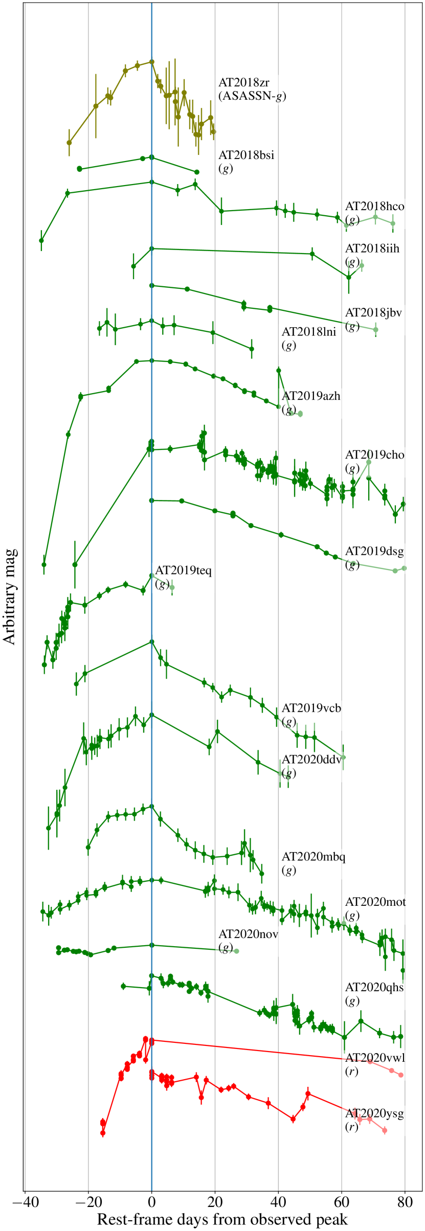
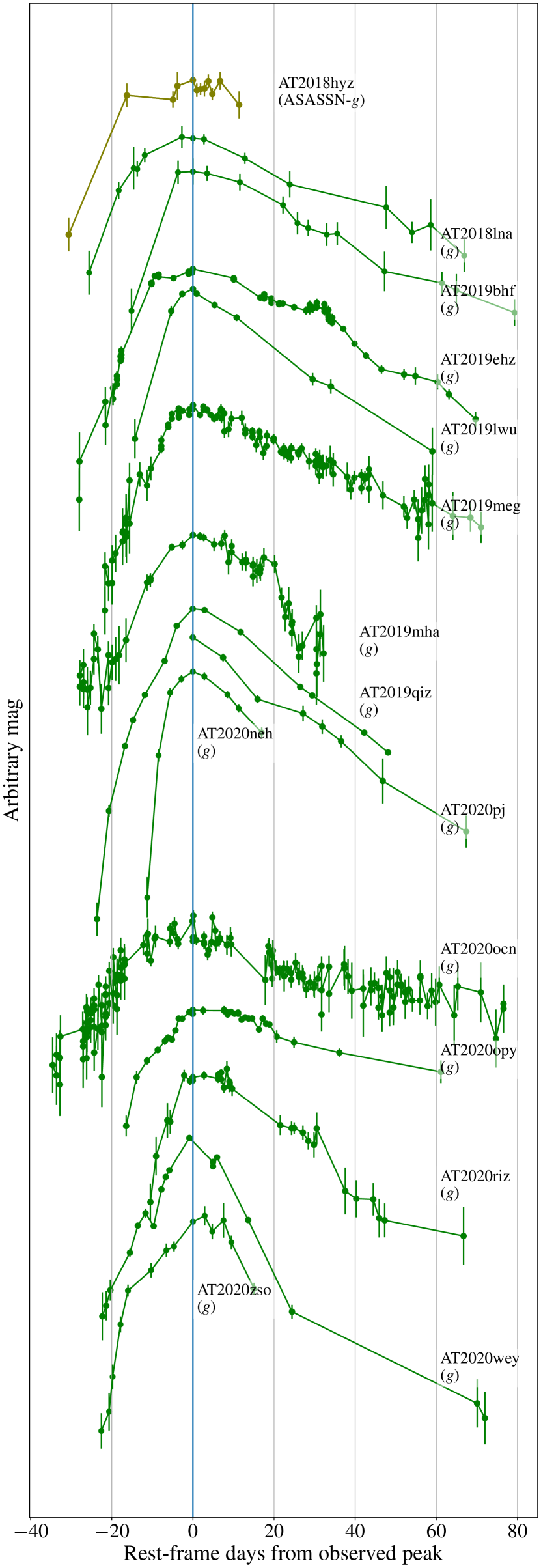
Figure 1: Light curves around the peak for ZTF-I TDFs.

3 Blackbody Fitting

After collecting the photometric data of the 33 TDFs, we begin to fit the peak SED of each source into a blackbody model. We use a simplest redshifted blackbody model, which only contains two free parameters: the temperature $T_{\rm bb}$ and radius $R_{\rm bb}$,

$$f_{\lambda}(\lambda)=\frac{2\pi hc^{2}}{\lambda^{5}}(1+z)^{4}\frac{1}{e^{hc(1+z)/\lambda kT_{\rm bb}}-1}\left(\frac{R_{\rm bb}}{D_{L}(z)}\right)^{2}.$$ (1)

Before the fitting, we determine the peaks by ZTF light curves except for AT2018zr, which peaked during the phase of reference image construction, and consequently the ZTF forced-photometry service can not provide the differential light curves around the peak. For this source we refer to van Velzen et al. (2019), in which the peak was carefully calibrated after the reconstruction of reference images. Then we extract the optical photometric data around the peak for each source.

To constrain the blackbody temperature more accurately, we also add the $Swift$ UVOT data into the SED fitting especially taking advantage of its unique UV photometry. As mentioned in Section 2.2, we have only selected UVOT bands with both late-time observations and significant variability to ensure a reliable measurement. These two selection criteria filter out sources that are not extensively covered by $Swift$ and result in 20 sources being followed sufficiently well in at least one UVOT band. Among them, 11 sources have UVOT coverage around ZTF peaks and the other 9 have only available observations in the declining phase. For the latter case, we assume that the $T_{\rm bb}$ evolves slowly, which is a common feature of TDE, hence the variation since peak should be negligible. The assumption is reasonable for most sources that were observed by UVOT $\sim 10-50$ days after their peaks. We fit these post-peak data, and use the resulting $T_{\rm bb}$ and the peak data to calculate the peak $R_{\rm bb}$.

For the remaining 13 sources, UV photometry is unfortunately absent. In order to minimize the impact of too few bands, we have taken ZTF $i$ band, ATLAS $c$ and $o$ bands and some LCOGT and ASAS-SN bands into consideration. However, the fitting to most sources still result in large uncertainties. We note that AT2020ysg is the only source whose peak can not be resolved, due to a large $\sim 80$-day gap around its intrinsic peak. In addition, its detected peak has only a single measurement, hence a post-peak fitting is still needed.

To get the two parameters, $T_{\rm bb}$ and $R_{\rm bb}$, for each source, we use the Markov chain Monte Carlo (MCMC) sampler emcee (Foreman-Mackey et al., 2013). We use 32 walkers and 5000 steps but discarding the first 2000 steps to ensure convergence. The best fitting results are presented in Table 2.

Table 2: Best fitting results for the blackbody model and maximum redshift

IAU	$Swift$	Fit	$T_{\rm bb}$	$R_{\rm bb}$	$L_{\rm bb}$	$L_{g}$	$z$	$z_{\rm max}$	$z_{\rm max}$	$z_{\rm max}$
Name	UVOT	Peak	($10^{4}$ K)	(log10 cm)	(log10 erg s-1)	(log10 erg s-1)		($r$=19.5)	($r$=20.0)	($r$=20.5)
AT2018zr	Y	N	1.4	15.3	43.9	43.6	0.075	0.197	0.250	0.317
AT2018bsi	Y	N	2.3	14.8	43.9	43.1	0.051	0.104	0.133	0.170
AT2018hco	Y	N	2.3	14.9	44.1	43.4	0.088	0.141	0.180	0.231
AT2018hyz	Y	Y	1.8	15.1	44.1	43.6	0.046	0.192	0.245	0.314
AT2018iih	N	Y	3.4	15.1	45.2	44.0	0.212	0.314	0.413	0.551
AT2018jbv	Y	N	3.2	15.2	45.3	44.2	0.340	0.412	0.547	0.739
AT2018lni	N	Y	3.8	14.8	44.8	43.5	0.138	0.138	0.169	0.218
AT2018lna	Y	N	3.5	14.7	44.4	43.2	0.091	0.114	0.146	0.187
AT2019bhf	N	Y	2.5	14.9	44.3	43.4	0.121	0.158	0.202	0.261
AT2019cho	N	Y	2.4	15.0	44.3	43.5	0.193	0.193	0.216	0.279
AT2019azh	Y	Y	2.7	14.9	44.3	43.4	0.022	0.142	0.182	0.234
AT2019dsg	Y	Y	2.8	14.7	44.0	43.1	0.051	0.093	0.118	0.151
AT2019ehz	Y	Y	2.1	14.9	43.9	43.2	0.074	0.122	0.155	0.198
AT2019lwu	N	Y	1.7	15.1	43.8	43.4	0.117	0.145	0.185	0.236
AT2019meg	Y	N	2.5	14.9	44.3	43.4	0.152	0.154	0.197	0.254
AT2019mha	N	Y	1.6	15.1	43.8	43.3	0.148	0.148	0.184	0.234
AT2019qiz	Y	Y	1.8	14.8	43.5	42.9	0.015	0.079	0.100	0.128
AT2019teq	N	Y	1.2	15.0	43.3	43.0	0.088	0.097	0.123	0.155
AT2019vcb	N	Y	1.3	15.1	43.6	43.3	0.089	0.143	0.181	0.229
AT2020pj	N	Y	1.1	15.0	43.2	42.9	0.068	0.095	0.119	0.151
AT2020ddv	N	Y	3.4	14.8	44.6	43.4	0.160	0.160	0.189	0.244
AT2020ocn	Y	N	3.9	14.3	43.9	42.5	0.070	0.070	0.070	0.083
AT2020mbq	N	Y	1.4	15.0	43.5	43.2	0.093	0.115	0.146	0.185
AT2020mot	Y	Y	2.2	14.9	43.9	43.2	0.070	0.112	0.142	0.182
AT2020neh	Y	Y	1.7	15.0	43.7	43.2	0.062	0.123	0.156	0.199
AT2020nov	Y	Y	1.4	15.3	44.0	43.6	0.084	0.185	0.234	0.297
AT2020opy	Y	Y	1.7	15.2	44.1	43.6	0.159	0.197	0.251	0.321
AT2020qhs	Y	N	2.7	15.3	45.1	44.2	0.345	0.401	0.529	0.705
AT2020riz	N	Y	4.4	15.1	45.6	44.2	0.435	0.435	0.496	0.676
AT2020wey	Y	Y	2.6	14.4	43.3	42.4	0.027	0.046	0.058	0.074
AT2020vwl	Y	N	2.2	14.7	43.6	42.9	0.035	0.077	0.097	0.124
AT2020ysg	N	N	4.7	15.1	45.6	44.1	0.277	0.386	0.517	0.709
AT2020zso	Y	Y	1.8	15.0	43.9	43.3	0.061	0.128	0.163	0.208

Note. — Explanations for the columns:

1. $Swift$ UVOT: If the blackbody model fitting uses any reliable $Swift$ UVOT differential photometry (Y = yes, N = no).

2. Fit peak: If the blackbody model fitting is based on the photometry around the peak. Except AT2020ysg, all peaks are resolved, but some are either better sampled or followed by $Swift$ UVOT $\sim 10-80$ days later, therefore we use the late-time observations to fit the blackbody temperature, then fix the temperature and fit the data around the peak to get the radius. Yes (Y) for fitting on the peak, no (N) for fitting on late-time observations.

3. $L_{g}$: The rest-frame $g$-band luminosity.

4. $z_{\rm max}$: The maximum redshift where this TDF could have been detected given the ZTF $r$-band effective limiting magnitude. It should not be less than $z$.

4 Luminosity Function

After obtaining the peak blackbody parameters for each TDF in the ZTF-I sample, we can construct a peak LF with them. For a survey of sources with a constant flux, the LF can be estimated by weighting each source by the maximum volume, $V_{\rm max}$, in which the source can be detected (Schmidt, 1968). For transients like TDFs, we are interested in their volumetric rate, i.e., the number of this kind of transients per cubic Mpc per year as a function of peak luminosity.

4.1 ZTF-I TDF LF

We calculate the $V_{\rm max}$ as follows. First, we determine the limiting magnitude. Since the ZTF-I TDFs are selected by $g-r<0$, the detection is limited by the $r$-band magnitude. The distribution of $r$-band magnitude indicates the limiting magnitude for $r$-band should be around $19.5\lesssim r\lesssim 20.5$. We set three limiting magnitudes: $r=19.5$, 20.0 and 20.5. For each limiting magnitude, we use the blackbody model parameters to calculate the maximum redshift $z_{\rm max}$ for each source. Meanwhile, we calculate the rest-frame peak luminosity in $g$ band, $L_{g}$. We show the $z_{\rm max}$ and $L_{g}$ in Table 2.

After that, we set the survey area. The distribution of right ascension (R.A.) and declination (Dec.) for 33 TDFs yields a survey area of $A\approx 15000$ deg². Next, the survey duration is set as $\tau=2.7$ yr. Finally, we get the volumetric rate $\dot{N}$ for each source.

Now we can build the luminosity function. We look into two kinds of luminosity: one is the rest-frame $g$-band peak luminosity, $L_{g}$, while the other one is the blackbody luminosity, $L_{\rm bb}$.

4.1.1 LF for $L_{g}$

For $L_{g}$, we first bin them into eight bins separated by equivalent log $L_{g}$, then sum up the $\dot{N}$ for each bin. The error for volumetric rate in each bin is estimated based on bootstrapping.

We use a power-law model to fit the volumetric rate as a function of $L_{g}$:

$$\frac{d\dot{N}}{d\ {\rm log}_{10}L_{g}}=\dot{N}_{0}\left(\frac{L_{g}}{L_{g,0}}\right)^{a}.$$ (2)

For $L_{g,0}=10^{43}$ erg s^-1, a least-square fit yields:

1. For $r=19.5$, $\dot{N}_{0}=(7.8\pm 2.2)\times 10^{-8}$ Mpc^-3 yr^-1, $a=-1.28\pm 0.22$.

2. For $r=20.0$, $\dot{N}_{0}=(4.1\pm 1.1)\times 10^{-8}$ Mpc^-3 yr^-1, $a=-1.30\pm 0.21$.

3. For $r=20.5$, $\dot{N}_{0}=(2.1\pm 0.6)\times 10^{-8}$ Mpc^-3 yr^-1, $a=-1.33\pm 0.20$.

We notice the curves resemble a Schechter function (Schechter, 1976), so we also fit each curve into a Schechter-like function, defined as

$$\frac{d\dot{N}}{d\ {\rm log}_{10}L_{g}}=\dot{N}_{0}^{*}\left(\frac{L_{g}}{L_{g}^{*}}\right)^{\alpha}{\rm exp}\left(-\frac{L_{g}}{L_{g}^{*}}\right).$$ (3)

The fitting results are as follows:

1. For $r=19.5$, ${\rm log}\,\dot{N}_{0}^{*}\,$(Mpc${}^{-3}\,$yr${}^{-1})=-7.62\pm 0.23$, ${\rm log}\,L_{g}^{*}\,$(erg s^-1)$\,=43.82\pm 0.14$, $\alpha=-0.76\pm 0.11$.

2. For $r=20.0$, ${\rm log}\,\dot{N}_{0}^{*}\,$(Mpc${}^{-3}\,$yr${}^{-1})=-8.01\pm 0.26$, ${\rm log}\,L_{g}^{*}\,$(erg s^-1)$\,=43.87\pm 0.15$, $\alpha=-0.85\pm 0.11$.

3. For $r=20.5$, ${\rm log}\,\dot{N}_{0}^{*}\,$(Mpc${}^{-3}\,$yr${}^{-1})=-8.34\pm 0.27$, ${\rm log}\,L_{g}^{*}\,$(erg s^-1)$\,=43.88\pm 0.16$, $\alpha=-0.89\pm 0.11$.

The results are plotted in the left panel of Figure 2.

4.1.2 LF for $L_{bb}$

For $L_{\rm bb}$, we first bin them into seven bins separated by equivalent log $L_{\rm bb}$, then sum up the $\dot{N}$ for each bin. The error for volumetric rate in each bin is estimated based on bootstrapping.

We use a power-law model to fit the volumetric rate as a function of $L_{\rm bb}$:

$$\frac{d\dot{N}}{d\ {\rm log}_{10}L_{\rm bb}}=\dot{N}_{0}\left(\frac{L_{\rm bb}}{L_{{\rm bb},0}}\right)^{a}.$$ (4)

For $L_{{\rm bb},0}=10^{44}$ erg s^-1, a least-square fit yields:

1. For $r=19.5$, $\dot{N}_{0}=(3.0\pm 0.9)\times 10^{-8}$ Mpc^-3 yr^-1, $a=-1.22\pm 0.17$.

2. For $r=20.0$, $\dot{N}_{0}=(1.6\pm 0.5)\times 10^{-8}$ Mpc^-3 yr^-1, $a=-1.23\pm 0.17$.

3. For $r=20.5$, $\dot{N}_{0}=(8.2\pm 2.6)\times 10^{-9}$ Mpc^-3 yr^-1, $a=-1.26\pm 0.16$.

The results are plotted in the right panel of Figure 2.

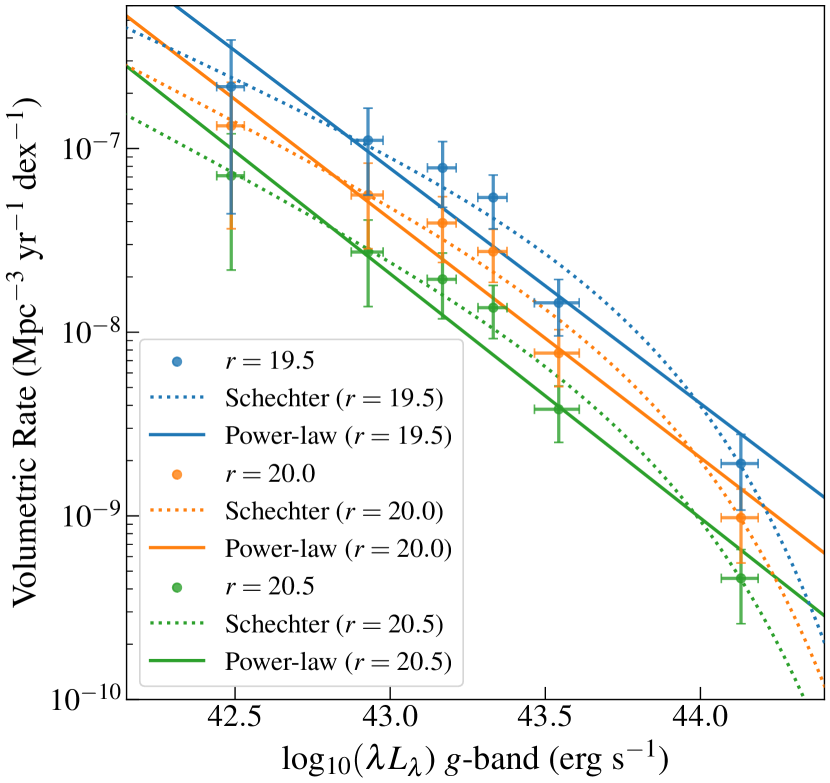
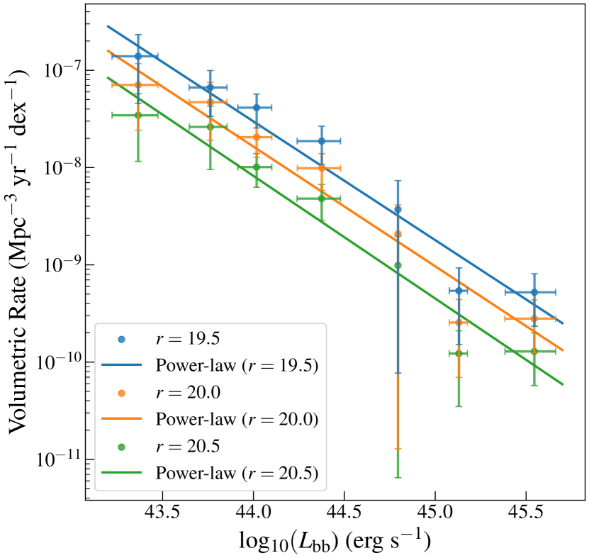
Figure 2: The TDF LF based on 33 ZTF-I TDFs. The volumetric rates for $r$-band limiting magnitudes $r=19.5$, $20.0$ and $20.5$ are shown in blue, orange and green, respectively. The solid and dotted lines represent the fitting results to a power-law profile and a Schechter function, respectively. The error for volumetric rate in each bin is estimated based on bootstrapping. Left: LF for rest-frame $g$-band peak luminosity $L_{g}$. The sources are binned into eight bins separated by equivalent log $L_{g}$. The number of sources in these eight bins is {2, 0, 4, 6, 8, 8, 0, 5}. Right: LF for blackbody luminosity $L_{\rm bb}$. The sources are binned into seven bins separated by equivalent log $L_{\rm bb}$. The number of sources in these seven bins is {5, 7, 9, 6, 1, 2, 3}.

4.2 Comparison with Previous LF

Our procedures for constructing LFs are not identical with the previous LF. For comparison, we follow the procedures of van Velzen (2018) to construct another set of LFs. We adopt the ”1/$\mathcal{V}_{\rm max}$” method, in which $\mathcal{V}_{\rm max}$ is defined as

$$\mathcal{V}_{\rm max}\equiv V(z_{\rm max})\ A_{\rm survey}\times\tau_{\rm survey}.$$ (5)

In this equation, $V(z_{\rm max})$ represents the volume per unit solid angle corresponding to the maximum redshift, while $A_{\rm survey}\times\tau_{\rm survey}$ denotes the product of the effective survey duration and survey area. To estimate the maximum redshift, the flux limit or limiting magnitude for ZTF must be decided. We use the same set of limiting magnitudes: $r=19.5$, 20.0 and 20.5. After that, we define a typical TDF as a flare with a peak luminosity of $L_{g}^{*}=10^{42.5}$ erg s^-1 and temperature $T_{\rm bb}^{*}=2.5\times 10^{4}$ K, so that we can use the formula

$$N_{\rm TDF,detected}\approx\dot{N}^{*}\times V(z_{\rm max}^{*})\ A_{\rm survey}\times\tau_{\rm survey}$$ (6)

to estimate the product of the effective survey duration and survey area $A_{\rm survey}\times\tau_{\rm survey}$. In this formula, the detected TDF number is $N_{\rm TDF,detected}=33$, while the mean volumetric rate $\dot{N}^{*}$ is set as $5\times 10^{-7}$ Mpc^-3 yr^-1 following van Velzen (2018). The $z_{\rm max}^{*}$ for $r=19.5$, $r=20.0$ and $r=20.5$ are 0.052, 0.066 and 0.084, respectively.

We use the blackbody model parameters and the limiting magnitudes to calculate $L_{g}$ and $z_{\rm max}$ for each source. The results are presented in Table 2. Next, we calculate $1/\mathcal{V}_{\rm max}$ for each source. We again look into two kinds of luminosity: $L_{g}$ and $L_{\rm bb}$. However, van Velzen (2018) only provides the LF for $L_{g}$. Therefore, we first rebuild this LF, then use the blackbody parameters provided in Table 1 of van Velzen (2018) to build the LF for $L_{\rm bb}$.

4.2.1 LF for $L_{g}$

For $L_{g}$, we bin all 33 ZTF-I TDFs into eight bins separated by equivalent log $L_{g}$, and sum up all $1/\mathcal{V}_{\rm max}$ in each bin. The uncertainties are estimated by $\sqrt{\sum 1/\mathcal{V}_{\rm max}^{2}}$. For $r=19.5$, the sum of $1/\mathcal{V}_{\rm max}$ for all 33 TDFs yields a rate of $6.3\times 10^{-8}$ Mpc^-3 yr^-1, one order of magnitude lower than the rate based on 13 TDFs, $8\times 10^{-7}$ Mpc^-3 yr^-1. In the left panel of Figure 3, we plot our result and the result of van Velzen (2018) for comparison. The result indicates no correlation between the volumetric rate and the limiting magnitude, i.e., the volumetric rates for $r=19.5$, 20.0 and 20.5 are almost the same. According to van Velzen et al. (2020), the single-epoch depth and filters of ZTF are similar to iPTF. Hence we adopt $r=19.5$, which is the effective limiting magnitude for iPTF in van Velzen (2018), for the following model fitting.

We use a power-law model to fit the volumetric rate as a function of $L_{g}$:

$$\frac{d\dot{N}}{d\ {\rm log}_{10}L_{g}}=\dot{N}_{0}\left(\frac{L_{g}}{L_{g,0}}\right)^{a}.$$ (7)

For $L_{g,0}=10^{43}$ erg s^-1, a least-square fit yields $\dot{N}_{0}=(5.1\pm 1.5)\times 10^{-8}$ Mpc^-3 yr^-1, $a=-1.28\pm 0.22$.

For comparison, van Velzen (2018) provided the fitting results. Notably, ASASSN-15lh is an exceptionally bright source among these 13 TDFs, superluminous yet with debating nature (e.g., Dong et al., 2016; Dai et al., 2016; Leloudas et al., 2016). Therefore, model fitting parameters for samples with and without ASASSN-15lh are both provided. For samples with ASASSN-15lh, $a=-1.6\pm 0.2$, $\dot{N}_{0}=(1.9\pm 0.7)\times 10^{-7}$ Mpc^-3 yr^-1. While for samples without ASASSN-15lh, $a=-1.3\pm 0.3$, $\dot{N}_{0}=(2.3\pm 0.8)\times 10^{-7}$ Mpc^-3 yr^-1. Although the index $a$ is well consistent with the previous LF without ASASSN-15lh, it is higher than the previous LF with ASASSN-15lh, and the average of $\dot{N}_{0}$ is a factor of $\sim$5 lower than both previous LFs. Nonetheless, these differences are at $\sim 2\sigma$ level.

Alternatively, a Gaussian model

$$\frac{d\dot{N}}{d\ {\rm log}_{10}L_{g}}=\dot{N}_{0}^{\prime}\ {\rm exp}\left\{-\frac{{[\rm log}_{10}(L_{g}/L_{g,0}^{\prime})]^{2}}{2b^{2}}\right\}$$ (8)

with $\dot{N}_{0}^{\prime}=1.0\times 10^{-7}$ Mpc^-3 yr^-1, $L_{g,0}^{\prime}=10^{42.5}$ erg s^-1 and $b=0.54$ provides a more reasonable description for the LF. For comparison, van Velzen (2018) used $\dot{N}_{0}^{\prime}=1.0\times 10^{-6}$ Mpc^-3 yr^-1, $L_{g,0}^{\prime}=10^{42.5}$ erg s^-1 and $b=0.4$ to describe the LF for TDFs without ASASSN-15lh.

In the left panel of Figure 3 we show the results for $r=19.5$, 20.0, 20.5 and van Velzen (2018). We will discuss these features in Section 5.

4.2.2 LF for $L_{bb}$

For $L_{\rm bb}$, we bin all 33 ZTF-I TDFs into seven bins separated by equivalent log $L_{\rm bb}$, and sum up all $1/\mathcal{V}_{\rm max}$ in each bin. The uncertainties are estimated by $\sqrt{\sum 1/\mathcal{V}_{\rm max}^{2}}$. For comparison, we use the blackbody parameters provided in Table 1 of van Velzen (2018) to build the LF for $L_{\rm bb}$. In the right panel of Figure 3, we plot the LFs for $L_{\rm bb}$ of ZTF-I and van Velzen (2018) TDFs. The ZTF-I TDF LFs again indicate no correlation between the volumetric rate and the limiting magnitude, hence we adopt $r=19.5$ for the following model fitting.

We use a power-law model to fit the volumetric rate as a function of $L_{\rm bb}$:

$$\frac{d\dot{N}}{d\ {\rm log}_{10}L_{\rm bb}}=\dot{N}_{0}\left(\frac{L_{\rm bb}}{L_{\rm{bb,0}}}\right)^{a}.$$ (9)

For $L_{\rm{bb,0}}=10^{44}$ erg s^-1, a least-square fit yields:

1. For ZTF-I TDFs, $\dot{N}_{0}=(1.9\pm 0.6)\times 10^{-8}$ Mpc^-3 yr^-1, $a=-1.22\pm 0.18$.

2. For van Velzen (2018) TDFs with ASASSN-15lh, $\dot{N}_{0}=(2.5\pm 1.0)\times 10^{-7}$ Mpc^-3 yr^-1, $a=-1.89\pm 0.21$.

3. For van Velzen (2018) TDFs without ASASSN-15lh, $\dot{N}_{0}=(2.8\pm 1.1)\times 10^{-7}$ Mpc^-3 yr^-1, $a=-1.51\pm 0.42$.

The LF of ZTF-I TDFs is much shallower than that of van Velzen (2018) TDFs. In the right panel of Figure 3 we show the results for $r=19.5$, 20.0, 20.5 and van Velzen (2018). We will discuss these features in Section 5.

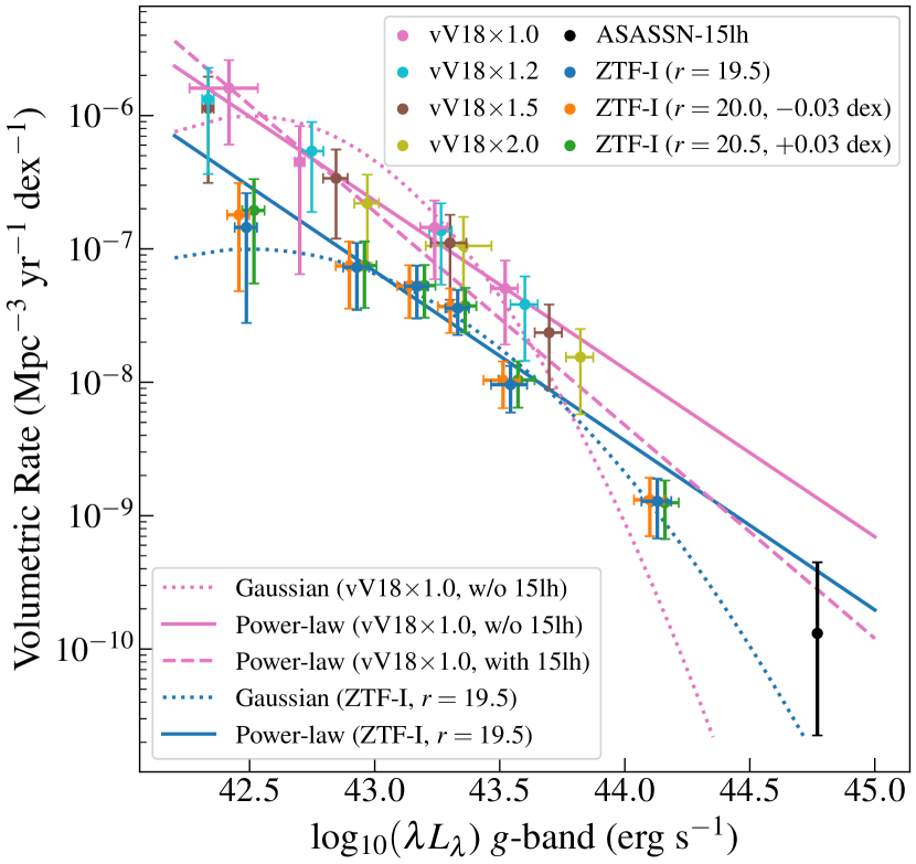
Figure 3: The TDF LF based on 33 ZTF-I TDFs following the procedures of van Velzen (2018). The volumetric rates for limiting magnitudes $r=19.5$, 20.0 and 20.5 are shown in blue, orange and green, respectively. The orange and green markers are slightly shifted for the convenience of display. The blue solid and dashed represents the fitting result to a power-law and a Gaussian model for $r=19.5$, respectively. For comparison, the previous TDF LF by van Velzen (2018) based on 13 TDFs is displayed in pink. Remarkably, the brightest source among 13 TDFs, ASASSN-15lh, is marked in black. It is outstandingly bright while its origin remains unclear. Therefore, we adopt the fitting parameters for both with and without (w/o) this source.
As 7 out of 13 TDFs in van Velzen (2018) have only post-peak light curves, their $z_{\rm max}$ should be underestimated. Consequently, their volumetric rates are overestimated. To evaluate this effect, we multiply their peak luminosity for a factor of 1.2, 1.5, 2.0. The data points and error bars in pink, cyan, brown and olive correspond to multiplication factors ($\times$) of 1.0, 1.2, 1.5 and 2.0, respectively. Left: LF for rest-frame $g$-band peak luminosity $L_{g}$. The sources are binned into eight bins separated by equivalent log $L_{g}$. The number of sources in these eight bins is {2, 0, 4, 6, 8, 8, 0, 5}. While for the sources of van Velzen (2018), the sources are binned into seven bins separated by equivalent log $L_{g}$. The number of sources in these seven bins for the multiplication factor of 1.0 (pink) is {4, 2, 3, 3, 0, 0, 1}. When the multiplication factors for post-peak sources are applied, the original power-law profile (solid and dashed pink line) can still describe the LF, while the Gaussian profile (dashed pink line) can not. Right: LF for blackbody luminosity $L_{\rm bb}$. The sources are binned into seven bins separated by equivalent log $L_{\rm bb}$. The number of sources in these seven bins is {5, 7, 9, 6, 1, 2, 3}. While for the sources of van Velzen (2018), the sources also are binned into seven bins separated by equivalent log $L_{\rm bb}$. The number of sources in these seven bins for the multiplication factor of 1.0 (pink) is {2, 4, 4, 2, 0, 0, 1}. When the multiplication factors for post-peak sources are applied, the original power-law profile (solid and dashed pink line) can still describe the LF.

5 Discussions

5.1 Shape of the LF

First, we discuss the shape of the LF. The ZTF-I TDF LF for $L_{g}$ can be described by a power-law profile, $dN/dL_{g}\propto L_{g}^{-2.3\pm 0.2}$. This is consistent with the previous van Velzen (2018) LF ($dN/dL_{g}\propto L_{g}^{-2.6\pm 0.2}$ for all 13 TDFs, $dN/dL_{g}\propto L_{g}^{-2.3\pm 0.3}$ if ASASSN-15lh is excluded). Additionally, it can be well described by a Schechter-like function. While for $L_{\rm bb}$, it can also be described by a power-law profile, $dN/dL_{\rm bb}\propto L_{\rm bb}^{-2.2\pm 0.2}$. This is shallower than the van Velzen (2018) LF ($dN/dL_{\rm bb}\propto L_{\rm bb}^{-2.9\pm 0.2}$ for all 13 TDFs, $dN/dL_{\rm bb}\propto L_{\rm bb}^{-2.5\pm 0.4}$ if ASASSN-15lh is excluded).

At the low-luminosity end, the LF for $L_{g}$ flattens at $L_{g}\sim 10^{42.5-43.0}$ erg s^-1. Given a bolometric correction of $\sim 10$, it corresponds to the Eddington luminosity for BHs with mass $M_{\rm BH}=10^{5.5-6.0}\ M_{\odot}$. This is consistent with an Eddington-limited emission scenario. However, a power-law profile can still fit this end due to the large errors, and the LF for $L_{\rm bb}$ does not flatten at low luminosity. Hence, more faint samples are needed to reach a final judgment.

While at the high-luminosity end, 5 bright sources constrain the volumetric rate at $L_{g}\sim 10^{44.0-44.3}$ erg s^-1 and $L_{\rm bb}\sim 10^{45.0-45.7}$ erg s^-1, indicating a suppression of volumetric rate in this range. This corresponds to the Eddington limit for BHs with $M_{\rm BH}\gtrsim 10^{7}\ M_{\odot}$. The TDF can only be created when the tidal radius ($R_{\rm t}$) equals or surpasses the innermost bound circular orbit (IBCO) of the black hole, i.e., $R_{\rm t}\gtrsim R_{\rm IBCO}$, indicating a maximum black hole mass, or the Hills mass. For non-spinning BHs,

$$M_{\rm Hills}=9.0\times 10^{7}\,M_{\odot}\left(\frac{M_{\star}}{M_{\odot}}\right)^{-1/2}\left(\frac{R_{\star}}{R_{\odot}}\right)^{3/2}$$ (10)

(Hills, 1975; Beloborodov et al., 1992; Leloudas et al., 2016). This indicates a rate suppression around $L_{g}\sim 10^{45}$ erg s^-1 and $L_{\rm bb}\sim 10^{46}$ erg s^-1 for sun-like stars. However, the vast majority of stars should be sub-solar main sequence stars, which obey $M_{\rm Hills}\propto M_{\star}^{0.7}$ (Stone & Metzger, 2016; Lin et al., 2022). Therefore, the average Hills mass should be lower, yielding a more consistent, lower luminosity. The above result agrees with the recent calculation of Coughlin & Nixon (2022), which indicates a rate suppression for BHs with $M_{\rm BH}>10^{7}\ M_{\odot}$, given a predominantly low-mass stellar population.

5.2 Volumetric Rate

As introduced in Section 4.2, the sum of $1/\mathcal{V}_{\rm max}$ for all 33 TDFs yields a rate of $6.3\times 10^{-8}$ Mpc^-3 yr^-1, that is one order of magnitude lower than the rate inferred from the 13 TDFs in van Velzen (2018), $8\times 10^{-7}$ Mpc^-3 yr^-1. Note that 7 out of 13 TDFs have only post-peak light curves, which will certainly lead to an overestimate of the volumetric rate. In order to assess the impact of these post-peak TDFs, for each source that only has post-peak data, we multiply the $L_{g}$ and $L_{\rm bb}$ by factors of 1.2, 1.5 and 2.0, respectively. Then we recalculate new $z_{\rm max}$ and the $\mathcal{V}_{\rm max}$ for each multiplication factor. Finally, we add up the $1/\mathcal{V}_{\rm max}$ and get new LFs. The results are shown in Figure 3.

As displayed in Figure 3, if the true peak luminosity of all of the sources discovered after maximum light is higher than the observed maximum luminosity, the original Gaussian profile will not stand. However, the original power-law profile seems stable within the 1-$\sigma$ errors, while a systematically higher volumetric rate than the ZTF-I TDFs still remains. The sum of $1/\mathcal{V}_{\rm max}$ for all 13 TDFs that used for the LF yields a rate of (7.2, 6.6, 6.0) $\times 10^{-7}$ Mpc^-3 yr^-1 for factors of 1.2, 1.5 and 2.0. Therefore, we conclude that the sources detected after the peak only have limited effect on the volumetric rate.

We notice that the 13 sources are collected from 5 surveys ranging from 2004 to 2016, a normalization based on the TDF number is applied (Equation 6), the product of effective survey duration and survey area ($A\times\tau$) ranges from 17 deg² yr ($GALEX$) to 82637 deg² yr (ASAS-SN). As a result, the serendipity of the TDF discoveries may lead to a higher (or lower) volumetric rate. For example, the two SDSS TDFs contribute $1.3\times 10^{-7}$ and $8.6\times 10^{-9}$ Mpc^-3 yr^-1 to the total volumetric rate, while the two iPTF sources contribute $6.3\times 10^{-9}$ and $3.2\times 10^{-7}$ Mpc^-3 yr^-1 to the total volumetric rate. Limited by the TDF number of each survey, we can not decide whether this serendipity raises or suppresses the volumetric rate. The reason for the lower volumetric rate is still uncertain.

6 Conclusions

We have obtained the optical and blackbody LFs for the 33 TDFs discovered in the ZTF-I survey, which is the largest sample obtained in a systematic search up to now. In addition to a much larger sample size, majority of these TDFs have nice coverage around their luminosity peaks and have been continuously followed by $Swift$ observations. We have carefully calculated the rest-frame $g$-band luminosity $L_{g}$ and blackbody luminosity $L_{\rm bb}$ by blackbody fitting to the SEDs around peaks and then the LFs. For comparison, we also use the data of van Velzen (2018) sample to rebuild the optical LF, and build a blackbody LF. Our conclusions are summarized as follows.

1. The LF for $L_{g}$ can be described by a power-law profile, $dN/dL_{g}\propto L_{g}^{-2.3}$. This is consistent with the previous LF by van Velzen (2018), albeit the normalization factor $\dot{N}_{0}$ is $\sim 5$ times lower. It can also be well described by a Schechter-like function (Equation 3).

2. The LF for $L_{\rm bb}$ can be described by a power-law profile, $dN/dL_{\rm bb}\propto L_{\rm bb}^{-2.2}$, which is shallower than the LF of the van Velzen (2018) sample.

3. At the low-luminosity end, the flat profile at $L_{g}\sim 10^{42.5-43.0}$ erg s^-1 supports an Eddington-limited emission mechanism, as the luminosity corresponds to the Eddington luminosity for BHs with mass $M_{\rm BH}=10^{5.5-6.0}\ M_{\odot}$, given a bolometric correction of $\sim 10$. However, the blackbody LF does not show a corresponding flat profile.

4. At the high-luminosity end, the volumetric rate drops at $L_{g}>10^{44}$ erg s^-1 and $L_{\rm bb}>10^{45}$ erg s^-1, corresponding to the Eddington luminosity for BHs with $M_{\rm BH}\gtrsim 10^{7}\ M_{\odot}$. This is consistent with a rate suppression around the Hills mass.

5. The total volumetric rate is one order of magnitude lower than that given by van Velzen (2018). Correcting the peak luminosity for sources observed post peaks in van Velzen (2018) can not effectively eliminate the discrepancy. The previous LF construction might be yet greatly impacted by the serendipitous discoveries in the step of normalization of these surveys (Equation 6). However, how the serendipity affects volumetric rate in detail remains unclear due to the small number of TDFs in each survey.

The uniform, wide-field and high-cadence ZTF-I survey greatly benefits the systematical search for TDFs, and thus well reduces the serendipity and improves the reliability of the LFs. Upcoming similar but deeper surveys, for instance, by the Vera Rubin Observatory (VRO) and Wide-Field Survey Telescope (WFST), should unveil much more TDFs, especially further and fainter ones. Hence, they should pave the way to more accurate LFs, and better constrain the shape of the LFs, especially on the faint end, e.g., towards a power-law profile, a Schechter-like function, or other formats.

References

- Bade et al. (1996) Bade, N., Komossa, S., & Dahlem, M. 1996, A&A, 309, L35
- Bellm et al. (2019a) Bellm, E. C., Kulkarni, S. R., Graham, M. J., et al. 2019a, PASP, 131, 018002, doi: 10.1088/1538-3873/aaecbe
- Bellm et al. (2019b) Bellm, E. C., Kulkarni, S. R., Barlow, T., et al. 2019b, PASP, 131, 068003, doi: 10.1088/1538-3873/ab0c2a
- Beloborodov et al. (1992) Beloborodov, A. M., Illarionov, A. F., Ivanov, P. B., & Polnarev, A. G. 1992, MNRAS, 259, 209, doi: 10.1093/mnras/259.2.209
- Bonnerot et al. (2016) Bonnerot, C., Rossi, E. M., & Lodato, G. 2016, MNRAS, 458, 3324, doi: 10.1093/mnras/stw486
- Bricman & Gomboc (2020) Bricman, K., & Gomboc, A. 2020, ApJ, 890, 73, doi: 10.3847/1538-4357/ab6989
- Brown et al. (2013) Brown, T. M., Baliber, N., Bianco, F. B., et al. 2013, PASP, 125, 1031, doi: 10.1086/673168
- Chambers et al. (2016) Chambers, K. C., Magnier, E. A., Metcalfe, N., et al. 2016, arXiv e-prints, arXiv:1612.05560. https://arxiv.org/abs/1612.05560
- Coughlin et al. (2017) Coughlin, E. R., Armitage, P. J., Nixon, C., & Begelman, M. C. 2017, MNRAS, 465, 3840, doi: 10.1093/mnras/stw2913
- Coughlin & Nixon (2022) Coughlin, E. R., & Nixon, C. J. 2022, ApJ, 936, 70, doi: 10.3847/1538-4357/ac85b3
- Dai et al. (2018) Dai, L., McKinney, J. C., Roth, N., Ramirez-Ruiz, E., & Miller, M. C. 2018, ApJ, 859, L20, doi: 10.3847/2041-8213/aab429
- Dai et al. (2016) Dai, Z. G., Wang, S. Q., Wang, J. S., Wang, L. J., & Yu, Y. W. 2016, ApJ, 817, 132, doi: 10.3847/0004-637X/817/2/132
- Dong et al. (2016) Dong, S., Shappee, B. J., Prieto, J. L., et al. 2016, Science, 351, 257, doi: 10.1126/science.aac9613
- Foreman-Mackey et al. (2013) Foreman-Mackey, D., Hogg, D. W., Lang, D., & Goodman, J. 2013, PASP, 125, 306, doi: 10.1086/670067
- Gehrels et al. (2004) Gehrels, N., Chincarini, G., Giommi, P., et al. 2004, ApJ, 611, 1005, doi: 10.1086/422091
- Gezari (2021) Gezari, S. 2021, ARA&A, 59, 21, doi: 10.1146/annurev-astro-111720-030029
- Gomez et al. (2020) Gomez, S., Nicholl, M., Short, P., et al. 2020, MNRAS, 497, 1925, doi: 10.1093/mnras/staa2099
- Green (2018) Green, G. M. 2018, The Journal of Open Source Software, 3, 695, doi: 10.21105/joss.00695
- Guillochon et al. (2017) Guillochon, J., Parrent, J., Kelley, L. Z., & Margutti, R. 2017, ApJ, 835, 64, doi: 10.3847/1538-4357/835/1/64
- Guillochon & Ramirez-Ruiz (2015) Guillochon, J., & Ramirez-Ruiz, E. 2015, ApJ, 809, 166, doi: 10.1088/0004-637X/809/2/166
- Hammerstein et al. (2022) Hammerstein, E., van Velzen, S., Gezari, S., et al. 2022, arXiv e-prints, arXiv:2203.01461. https://arxiv.org/abs/2203.01461
- Hills (1975) Hills, J. G. 1975, Nature, 254, 295, doi: 10.1038/254295a0
- Holoien et al. (2016) Holoien, T. W. S., Kochanek, C. S., Prieto, J. L., et al. 2016, MNRAS, 455, 2918, doi: 10.1093/mnras/stv2486
- Ivezić et al. (2019) Ivezić, Ž., Kahn, S. M., Tyson, J. A., et al. 2019, ApJ, 873, 111, doi: 10.3847/1538-4357/ab042c
- Jiang et al. (2016) Jiang, Y.-F., Guillochon, J., & Loeb, A. 2016, ApJ, 830, 125, doi: 10.3847/0004-637X/830/2/125
- Leloudas et al. (2016) Leloudas, G., Fraser, M., Stone, N. C., et al. 2016, Nature Astronomy, 1, 0002, doi: 10.1038/s41550-016-0002
- Lin et al. (2022) Lin, Z., Jiang, N., & Kong, X. 2022, MNRAS, 513, 2422, doi: 10.1093/mnras/stac946
- Lu & Bonnerot (2020) Lu, W., & Bonnerot, C. 2020, MNRAS, 492, 686, doi: 10.1093/mnras/stz3405
- Masci et al. (2019) Masci, F. J., Laher, R. R., Rusholme, B., et al. 2019, PASP, 131, 018003, doi: 10.1088/1538-3873/aae8ac
- Merritt & Poon (2004) Merritt, D., & Poon, M. Y. 2004, ApJ, 606, 788, doi: 10.1086/382497
- Metzger & Stone (2016) Metzger, B. D., & Stone, N. C. 2016, MNRAS, 461, 948, doi: 10.1093/mnras/stw1394
- Nicholl et al. (2020) Nicholl, M., Wevers, T., Oates, S. R., et al. 2020, MNRAS, 499, 482, doi: 10.1093/mnras/staa2824
- Oke (1974) Oke, J. B. 1974, ApJS, 27, 21, doi: 10.1086/190287
- Piran et al. (2015) Piran, T., Svirski, G., Krolik, J., Cheng, R. M., & Shiokawa, H. 2015, ApJ, 806, 164, doi: 10.1088/0004-637X/806/2/164
- Planck Collaboration et al. (2016) Planck Collaboration, Aghanim, N., Ashdown, M., et al. 2016, A&A, 596, A109, doi: 10.1051/0004-6361/201629022
- Rees (1988) Rees, M. J. 1988, Nature, 333, 523, doi: 10.1038/333523a0
- Roming et al. (2005) Roming, P. W. A., Kennedy, T. E., Mason, K. O., et al. 2005, Space Sci. Rev., 120, 95, doi: 10.1007/s11214-005-5095-4
- Roth et al. (2021) Roth, N., van Velzen, S., Cenko, S. B., & Mushotzky, R. F. 2021, ApJ, 910, 93, doi: 10.3847/1538-4357/abdf50
- Schechter (1976) Schechter, P. 1976, ApJ, 203, 297, doi: 10.1086/154079
- Schmidt (1968) Schmidt, M. 1968, ApJ, 151, 393, doi: 10.1086/149446
- Shappee et al. (2014) Shappee, B. J., Prieto, J. L., Grupe, D., et al. 2014, ApJ, 788, 48, doi: 10.1088/0004-637X/788/1/48
- Smith et al. (2020) Smith, K. W., Smartt, S. J., Young, D. R., et al. 2020, PASP, 132, 085002, doi: 10.1088/1538-3873/ab936e
- Stone & Metzger (2016) Stone, N. C., & Metzger, B. D. 2016, MNRAS, 455, 859, doi: 10.1093/mnras/stv2281
- Stone et al. (2020) Stone, N. C., Vasiliev, E., Kesden, M., et al. 2020, Space Sci. Rev., 216, 35, doi: 10.1007/s11214-020-00651-4
- Strubbe & Quataert (2009) Strubbe, L. E., & Quataert, E. 2009, MNRAS, 400, 2070, doi: 10.1111/j.1365-2966.2009.15599.x
- Thorp et al. (2019) Thorp, S., Chadwick, E., & Sesana, A. 2019, MNRAS, 488, 4042, doi: 10.1093/mnras/stz1970
- Tonry et al. (2018) Tonry, J. L., Denneau, L., Heinze, A. N., et al. 2018, PASP, 130, 064505, doi: 10.1088/1538-3873/aabadf
- van Velzen (2018) van Velzen, S. 2018, ApJ, 852, 72, doi: 10.3847/1538-4357/aa998e
- van Velzen & Farrar (2014) van Velzen, S., & Farrar, G. R. 2014, ApJ, 792, 53, doi: 10.1088/0004-637X/792/1/53
- van Velzen et al. (2020) van Velzen, S., Holoien, T. W. S., Onori, F., Hung, T., & Arcavi, I. 2020, Space Sci. Rev., 216, 124, doi: 10.1007/s11214-020-00753-z
- van Velzen et al. (2011) van Velzen, S., Farrar, G. R., Gezari, S., et al. 2011, ApJ, 741, 73, doi: 10.1088/0004-637X/741/2/73
- van Velzen et al. (2019) van Velzen, S., Gezari, S., Cenko, S. B., et al. 2019, ApJ, 872, 198, doi: 10.3847/1538-4357/aafe0c
- Wang & Merritt (2004) Wang, J., & Merritt, D. 2004, ApJ, 600, 149, doi: 10.1086/379767