Resonant anomaly detection without background sculpting

Abstract

We introduce a new technique named Latent CATHODE (LaCathode) for performing “enhanced bump hunts”, a type of resonant anomaly search that combines conventional one-dimensional bump hunts with a model-agnostic anomaly score in an auxiliary feature space where potential signals could also be localized. The main advantage of LaCathode over existing methods is that it provides an anomaly score that is well behaved when evaluating it beyond the signal region, which is essential to prevent the sculpting of background distributions in the bump hunt. LaCathode accomplishes this by constructing the anomaly score directly in the latent space learned by a conditional normalizing flow trained on sideband regions. We demonstrate the superior stability and comparable performance of LaCathode for enhanced bump hunting in an illustrative toy example as well as on the LHC Olympics R&D dataset.

I Introduction

Despite countless searches for new physics at the LHC, so far no evidence for physics beyond the Standard Model was found. The vast majority of these searches are model specific, motivated by and optimized for particular scenarios and particle spectra. Recently there has been much interest in the possibility that new physics could be present in the data but we simply have not searched in the right places yet. This has led to an enormous activity in developing new methods for model-agnostic searches at the LHC (see e.g. [1, 2] for recent community overviews of anomaly detection and [3] for a more general overview of machine learning methods to search for new physics).

One promising class of approaches can be referred to as “enhanced bump hunts”, where the idea is to upgrade a standard one-dimensional bump hunt, e.g. in an invariant mass $m$, to a multivariate setting. This is achieved by including an anomaly score $R(x)$ learned from auxiliary features $x\in{\mathbb{R}}^{d}$ where the signal may also be localized, but in an a priori unknown way.

In general, enhanced bump hunts follow these steps:

1. Designate nonoverlapping signal region (SR) and sidebands (SB) in $m$.

2. Derive an anomaly score $R(x)$ and select events that pass a threshold value $R(x)>R_{c}$.

3. Fit a suitable (e.g. falling spectrum) background-only function to the selected events in the SB.

4. Compare the background-only prediction from step iii) to data in the SR and derive limits or claim discovery.

Methods for enhanced bump hunts include those constructed using autoencoders [5, 6] or based on weak supervision [7, 8]. While weak supervision allows the construction (in an ideal case) of a provably optimal anomaly score—see Section II.1 for details—correlations between the bump hunt feature and auxiliary features can spoil these methods. This observation has motivated the development of a number of new techniques that aim to improve the sensitivity and stability of anomaly detection in the presence of correlations [9, 10, 11, 12, 13]. In particular, the recently proposed Cathode [12] and Curtains [13] techniques have been demonstrated to achieve close-to-optimal signal sensitivity, even in the presence of correlations between features.

This paper is concerned with another issue that has received less attention but still might spoil the practical application of enhanced bump hunts: background sculpting. The enhanced bump hunting procedure outlined above can only work if the cut introduced in ii) does not sculpt the background (i.e. introduce artificial bumps in the background-only $m$ spectrum). Alas, state-of-the-art protocols like Cathode and Curtains have no built-in measures to prevent such sculpting. Even worse, the anomaly score of these approaches is only derived for the SR, leading to potentially unpredictable extrapolation behavior elsewhere.

The scope of this paper is to clearly identify this sculpting issue and to provide a viable solution. In Sec. II, we first discuss enhanced bump hunt strategies and then introduce the novel LaCathode approach. Section III uses an analytic toy model to illustrate the problem and shows that correlations between $m$ and the auxiliary features are the root cause of background sculpting. It also shows that LaCathode indeed successfully mitigates this issue. Section IV reiterates these points, but in the context of the more physically motivated LHC Olympics R&D dataset [14]. Section V concludes this work.

II Method

II.1 Existing strategies for enhanced bump hunts

According to the Neyman-Pearson lemma [15], the provably optimal anomaly score for any model-agnostic search would be:

$$R(x)={p_{data}(x)\over p_{bg}(x)}$$ (1)

where $p_{data}(x)$ and $p_{bg}(x)$ are the probability densities of the data and the background respectively. Of course, in practice we never have access to this likelihood ratio, since the probability densities of data and background are in general intractable. At best, one could hope for a large number of samples drawn from the data and true background distributions; then one could approximate $R(x)$ with a classifier trained on these samples. We will refer to this approximation of (1) as the “idealized anomaly detector” throughout.

Since it is generally not possible to draw samples from the true $p_{bg}(x)$ in a realistic anomaly search scenario, we can at best approximate this idealized case either with simulations or in a data-driven way. The focus here will be on the latter strategy.

The challenge then is to obtain a high-quality estimate for $p_{bg}(x)$ from data, e.g. by interpolating from sidebands (SB) in $m$ into a signal region (SR), and use weak supervision to obtain an anomaly score $R(x)$. As long as a cut on $R(x)>R_{c}$ does not sculpt the $m$ distribution, one can combine this cut with the 1D bump hunt in $m$ to greatly enhance the significance of the signal over the background.

In the original enhanced bump hunt method, called CWoLa-Hunting [8], $R(x)$ comes from a SR vs SB classifier. This works as long as the features $x$ and $m$ are statistically independent in the background (i.e. the $x$ features are distributed identically in the SR and the SB for the background). This also ensures that $R(x)>R_{c}$ will not sculpt the $m$ distribution. Using these properties, the full enhanced bump hunt search strategy using CWoLa-Hunting was successfully demonstrated on toy simulation data  [8, 16], and then implemented on actual data by the ATLAS Collaboration in [17].

However, it can be challenging to ensure that $x$ and $m$ are independent in the background. Even a small correlation can degrade or destroy the sensitivity of CWoLa Hunting to anomalies. This has motivated the development of alternative approaches that are more robust to correlations.

• In Anode [9], one learns $p_{data}(x)$ and $p_{bg}(x)$ using conditional density estimators trained on the data with $m\in SR$ and with $m\in SB$; the latter are automatically interpolated in $m$ into the SR, which alleviates the problem with correlations between $x$ and $m$. It was shown in [12] that in the presence of correlations between $x$ and $m$, the signal sensitivity of Anode is robust while that of CWoLa-Hunting collapses.

• In Cathode [12], one learns $p_{bg}(x)$ using the SB density estimator just as in Anode. However, instead of the second SR density estimator (which will be more difficult to learn as it must also capture the tiny deviations from the smooth $p_{bg}(x)$ from a small localized signal), one samples from $p_{bg}(x)$ in the SR, and trains a classifier (as in CWoLa-Hunting) between the data and the synthetic background samples. Cathode thereby captures the best of both Anode and CWoLa-Hunting, achieving a signal sensitivity that is nearly optimal and yet robust to correlations between $x$ and $m$.

• Finally, the Curtains [13] protocol operates similar to Cathode, with the main difference that conditional invertible neural networks (cINNs) are used to map background examples from the SB into the SR.

II.2 The problem of background sculpting

So far, apart from CWoLa-Hunting, the majority of the effort has been invested in exploring data-driven approaches to learn $R(x)$ as accurately as possible from sidebands, while much less attention has been paid to the issue of background sculpting. However, signal sensitivity is not the only component of a successful new physics search; background estimation is also essential. In the presence of correlations between $x$ and $m$ in the background events, one must also show that $R(x)$, even if ideal, does not sculpt the background $m$ distribution around the signal region, which would prevent background estimation via the 1D bump hunt. See Fig. 1 for an illustration of such correlated input features.

Note that, in any complete enhanced bump hunt strategy, two data-driven background estimations must take place:

1. An interpolation of the learned $p_{bg}(x)$ from SB to SR in order to construct $R(x)$.

2. After cutting on $R(x)>R_{c}$, we proceed with the usual 1D bump hunt: an interpolation in the $m$ distribution from SB to SR (e.g. by fitting a suitable functional form to the data excluding the SR).

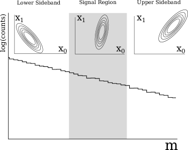
Figure 1: Illustration of the correlation of (hypothetical) input features $x_{0}$ and $x_{1}$ with $m$ in the background. This figure describes the situation mentioned in the text, where one can clearly observe that the background distributions of input features $x_{0}$ and $x_{1}$ change dramatically from the lower sideband (low $m$) to the upper sideband (high $m$) and thus are strongly correlated with $m$.

This work is concerned with ensuring the robustness of the second estimation. We will demonstrate—using both a simple analytic toy model and examples drawn from the LHC Olympics 2020 R&D dataset [14]—that in the presence of correlations between $x$ and $m$, cutting on the learned $R(x)$ can result in significant sculpting of the $m$ distribution. This can be understood by the fact that $R(x)$ must be a more-or-less smooth function of $x$, so any correlations of $m$ with $x$ will be inherited by $R(x)$. Furthermore, $R(x)$ was learned using events in the SR, so it has to be extrapolated from SR to SB in order to apply the threshold $R(x)>R_{c}$ everywhere. This extrapolation could lead to unpredictable effects, including sculpting, especially in the presence of strong correlations between $x$ and $m$.

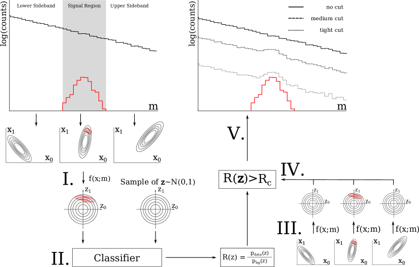
Figure 2: Flowchart describing the different steps of the proposed LaCathode method. First, one maps the data in the SR (denoted by the vertical gray band) to the latent space (I), and trains a classifier $R(z)$ to distinguish data from the background which follows the normal distribution (II). Then one maps all the data (in both SR and SB) to the latent space (III) and passes this through $R(z)$, selecting only those events above some threshold $R(z)>R_{c}$ (IV). Finally, one plots the $m$ distribution of the surviving events, and looks for a bump in the SR that would signify the presence of new physics (V).

II.3 LaCATHODE to the rescue

After identifying the issue that leads to sculpting of the background $m$ distribution, we present a solution to the problem, which is outlined in Fig. 2 and described in the following. We call our new approach Latent CATHODE or LaCathode for short, because it is closely derived from the Cathode method.

The solution actually lies at the heart of the Cathode method: the SB density estimator is a conditional normalizing flow, which is an invertible map $f$ from data space $x$ to a latent space $z$, for every value of $m$:

$$z=f(x;m)$$ (2)

The background events in the latent space $z$ are supposed to follow a simple prespecified base distribution, which we take to be the unit normal distribution ${\mathcal{N}}(\mu=0,\sigma=1)^{d}$ for concreteness.

The idea of LaCathode is to train the classifier between SR data and SR background in the latent space $z$ instead of in the physical feature space $x$. Since $f$ maps $x$ to the same latent space for every value of $m$, working in the latent space has the effect of decorrelating the data from $m$ in the background, which should eliminate the problem of sculpting. In other words, since the $z$ space is always the same for every $m$, no extrapolation is needed to evaluate $R(z)$ outside the SR where it was learned.

Furthermore, since $f$ is invertible, and likelihood ratios are invariant under coordinate reparametrizations, the $z$-space classifier should in principle be as asymptotically optimal as the $x$-space classifier, i.e.

$$R(x)={p_{data}(x)\over p_{bg}(x)}={p_{data}(z)\over p_{bg}(z)}=R(z)$$ (3)

The performance of the Cathode and LaCathode methods similarly rely on the quality of the trained and interpolated normalizing flow. For Cathode it controls the fidelity of the $p_{bg}(x)$ estimate, whereas for LaCathode the flow is responsible for $p_{data}(z)$. If the background events in data were not mapped to a unit normal distribution, both the learning of the likelihood ratio via the classifier and the decorrelation of auxiliary features from the resonant one would deteriorate.

We will show with examples in the following sections that LaCathode retains much of the excellent signal sensitivity as Cathode, while avoiding the sculpting of the $m$ distribution in the presence of correlations.

While LaCathode seems to be the superior enhanced bump hunting method, all is not lost for original Cathode—it remains a robust and powerful anomaly detection method as long as the correlations are sufficiently small. This is the case for the original feature set of the LHC Olympics 2020 R&D dataset—as discussed in [12], these have percent-level correlations with $m$, and we showed there that Cathode signal sensitivity remains robust to this small correlation (unlike CWoLa-Hunting, which is more fragile to correlations). In this paper we demonstrate that the $m$ distribution is also not sculpted after a cut on $R(x)$.

III Toy model

We begin by demonstrating the idea of LaCathode with a simple 1+2D toy model. In the first part, we will investigate how correlations between $x$ and $m$ affect the sculpting of $m$, and in the second part we will see what happens in the latent space.

The $m$ distribution will be sampled uniformly in the range $[-10,10]$. We will take the SR to be $m\in[-0.3,0.3]$. The $m$ distribution together with the SR is shown in Fig. 3.

The features $x$ will be sampled from ${\mathcal{N}}(\mu=c\times m,\sigma=1)^{2}$. The parameter $c$ controls the amount of correlation between $x$ and $m$. We will consider $c~{}\in~{}\{0.001,0.1\}$.

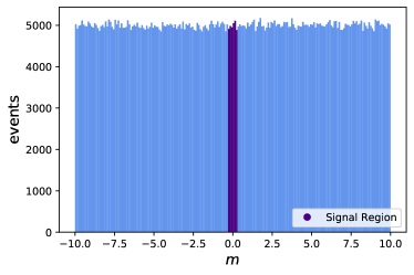
Figure 3: Uniform distribution of $m$, with signal region indicated in the darker band.

We generate two such sets, one “data” and one “sample”. Of the 1 million events generated in each set, half are reserved for training, 1/6 for validation, and the remaining events are used to evaluate the trained classifier.

A binary classifier is trained in the SR to distinguish “data” from “samples” in $x$ space. We find the cut values $R(x)>R_{c}$ that keep only the $1\%$ most anomalous events in the SR.

Although only trained in the SR, data on the entire interval $m\in[-10,10]$ are passed through the classifier and subject to the cut $R(x)>R_{c}$. If the classifier is not sculpting, it should return an $m$ distribution that looks uniform.

However, in the correlated case this is not necessarily what happens. Shown in the right column of Fig. 4 are the $m$ distributions after cuts on the classifier, for different values of the correlation $c$ and for three independently trained classifiers on the same toy dataset.

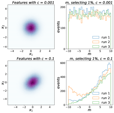
Figure 4: Features $x$ (left column) and the resulting $m$ distribution after a cut on the classifier score as described in the text (right column) under different correlations. The top row shows the case of a very small correlation, while the bottom row shows the features and results under a larger correlation.

If the correlation is very small ($c=0.001$), no sculpting is seen. Meanwhile, if the correlation is sufficiently large ($c=0.1$), we see a severe sculpting in $m$. In this case, the $x$ distributions in the SB can be out of distribution relative to those in the SR, as seen in the left column of Fig. 4. This can lead to unpredictable effects on the $m$ distribution after a cut on $R(x)>R_{c}$.

Next we turn to the latent space, which will be an illustration of the LaCathode concept using this analytic toy model. Here we assume a perfect normalizing flow, so the transformation to the latent space is just

$$z=x-cm.$$ (4)

As can be seen in Fig. 5, a classifier trained on the latent space data vs. samples will not show any sculpting in $m$. We conclude that, as must be the case, LaCathode eliminates the sculpting of $m$ after a cut on $R(z)>R_{c}$. This of course makes perfect sense since $z$ and $m$ are completely independent of one another.

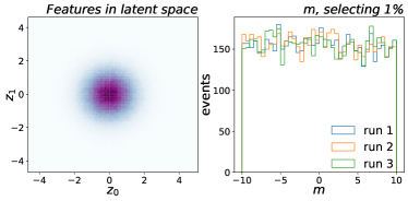
Figure 5: Features $z$ in latent space (left) and the resulting $m$ distribution after a cut on the classifier score as described in the text (right).

IV LHCO R&D dataset

Let us now consider a demonstration of LaCathode with the LHC Olympics R&D dataset [1, 14], where the resonant variable $m$ will be the dijet invariant mass $m_{JJ}$. For a description of the dataset and training details, refer to Appendix A. Additional information about the dataset can be found in [1, 12].

IV.1 Original features

To set the stage, here we demonstrate Cathode and LaCathode with the original feature set $x=(m_{1},\Delta m,\tau_{21}^{J_{1}},\tau_{21}^{J_{2}})$ of [9, 12].

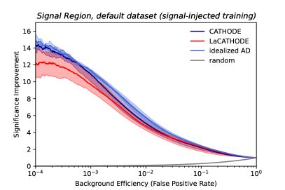
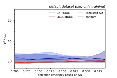
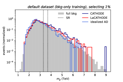
Figure 6: Performance comparison between Cathode, LaCathode and the idealized anomaly detector on the default dataset. The top left plot shows significance improvement in the SR as a function of background efficiency when training on the dataset with signal injected. The lines denote the median of ten independent retrainings whereas the bands show the central 68%. Similarly, the top right plot shows the distance between the distribution before and after a selection, quantified by the median and central 68% of the $\chi^{2}/n_{dof}$ metric, at continuous choices of selection efficiency. The denoted efficiency is based on the SR and the same anomaly score threshold is applied to the SB. In this case, the anomaly detectors were trained on pure background. The bottom plot shows the resulting normalized $m_{JJ}$ distributions, after selecting the 1% most anomalous events, based on the first of the ten background-only trainings, overlayed with the distribution before a cut. Overall, we see that for the original feature set, where correlations between the features and $m_{JJ}$ are small, the sculpting in original Cathode and the idealized AD in $x$ space are reasonably under control, although the variance in the $\chi^{2}$ distance metric is higher than for LaCathode.

First, we turn to Fig. 6 (top left), which shows the significance improvement characteristic (SIC) curves using the same injection as in [12], in terms of the median and the central 68% bands of ten independent trainings. Recall that the SIC is defined as the improvement in the nominal significance, $\epsilon_{S}/\sqrt{\epsilon_{B}}$, where $\epsilon_{S}$ and $\epsilon_{B}$ are the signal and background efficiencies in the SR, respectively, after a cut on the anomaly score. Unlike in [12], here we show the SIC as a function of the background efficiency. We see from Fig. 6 (top left) that LaCathode retains much of the signal sensitivity as original Cathode.

Shown in Fig. 6 (bottom) is the $m_{JJ}$ distribution for the original feature set for background events after cuts on $R(x)$, corresponding to keeping only the 1% most anomalous events within the SR. By eye, we see that there is only minimal sculpting.

In order to quantify this, we compute a histogram from the test data $m_{JJ}$ before selection corresponding to $n_{bins}=300$ bins with equal bin content ($N_{i}^{full}=N^{tot}/n_{bins}$ for each bin $i$) and normalize it to unit area $n_{i}^{full}=a_{i}N_{i}^{full}$. Here $n_{bins}$ has been chosen such that a 1% selection still retains at least ten test set events in every bin. After applying a selection of $\varepsilon_{sel}$ using an anomaly detector, the resulting $m_{JJ}$ is histogrammed with the same binning $N_{i}^{sel}$ and also normalized to unit area $n_{i}^{sel}=b_{i}N_{i}^{sel}$. One then obtains a distance metric $\chi^{2}$ as a function of decreasing $\varepsilon_{sel}$:

$$\chi^{2}=\sum_{i}\frac{\left(n_{i}^{full}-n_{i}^{sel}\right)^{2}}{\sigma_{i}^{2}}=\sum_{i}\frac{\left(n_{i}^{full}-n_{i}^{sel}\right)^{2}}{a_{i}^{2}\varepsilon_{sel}N_{i}^{full}}.$$ (5)

For better reference, the resulting $\chi^{2}$ is divided by the number of degrees of freedom $n_{dof}=n_{bins}-1$. This quantity is shown for Cathode, LaCathode and the idealized anomaly detector in Fig. 6 (top right), again in terms of the median and the central 68% bands of ten independent trainings. While all methods have values close to unity, both Cathode and the idealized anomaly detector have a higher variance than LaCathode, which overlaps for the most part with the $\chi^{2}$ that one obtains from 100 randomly drawn subsets of events with the target selection efficiency.

As in the toy example, this shows that Cathode can be robust against sculpting for small enough correlations. This means that as long as the features are well chosen, original Cathode can be a viable enhanced bump hunt method on its own, and superior to CWoLa-Hunting, which is more sensitive to correlations.

IV.2 Shifted features

Next, we show the sculpting with the shifted feature set $x^{\prime}=(m_{1}+cm_{JJ},\Delta m+cm_{JJ},\tau_{21}^{J_{1}},\tau_{21}^{J_{2}})$ where we choose $c=0.1$ as in [9, 12]. Now we observe in Fig. 7 that after cuts on $R(x)$ the sculpting is quite severe, again as expected from the toy model.

For LaCathode on the other hand, sculpting is still almost nonexistent after cuts on $R(z)$. This confirms what we found with the toy model (using now a trained normalizing flow and not a perfect one): the normalizing flow essentially decorrelates $z$ and $m_{JJ}$ and solves the problem of sculpting in the $m_{JJ}$ distribution.

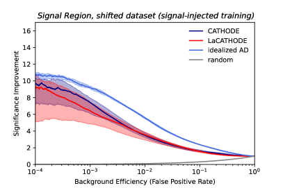
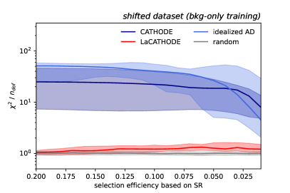
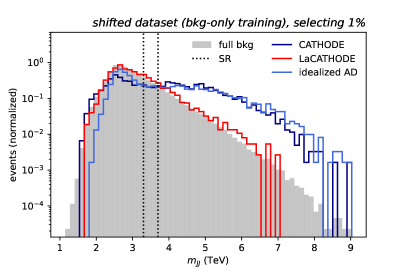
Figure 7: The same performance comparison between anomaly detectors as in Fig. 6, but trained and evaluated on the shifted dataset $x^{\prime}=(m_{1}+cm_{JJ},\Delta m+cm_{JJ},\tau_{21}^{J_{1}},\tau_{21}^{J_{2}})$ with $c=0.1$. Here we see much more significant sculpting in original Cathode and the idealized AD trained on $x$ space, while LaCathode is again completely stable to the cut on the anomaly score.

Figure 7 (top left) shows the SIC curves for LaCathode for the LHCO R&D signal with shifted features; we see that LaCathode more or less matches the original Cathode.

IV.3 Including $\Delta R$

Finally, we demonstrate the performance of Cathode and LaCathode in a somewhat more well-motivated feature set with correlations, i.e. including $\Delta R$. The angular distance $\Delta R$ between the two jets is defined as:

$$\Delta R=\sqrt{(\phi_{J_{2}}-\phi_{J_{1}})^{2}+(\eta_{J_{2}}-\eta_{J_{1}})^{2}}$$ (6)

This feature was first suggested in [13] as it might be relevant for certain signal models (e.g. due to different initial state radiation patterns compared to QCD jets) and because its strong correlation with the invariant mass introduces a well-motivated test of anomaly detection in the presence of correlations.

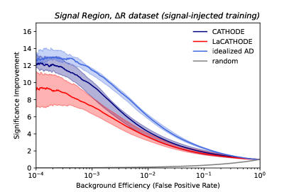
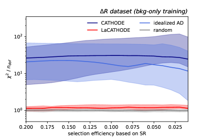
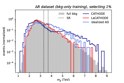
Figure 8: The same performance comparison between anomaly detectors as in Fig. 6, but trained and evaluated on the dataset $x^{\prime\prime}=(m_{1},\Delta m,\tau_{21}^{J_{1}},\tau_{21}^{J_{2}}$, $\Delta R)$. As in the case with the artificial correlations, we again see much more significant sculpting in original Cathode and the idealized AD trained on $x$ space, while LaCathode is once again completely stable to the cut on the anomaly score.

We see in Fig. 8 that Cathode has severe sculpting after cutting on $R(x)$, while LaCathode has essentially no sculpting. We see that in this case the signal sensitivity of LaCathode is lower than that of Cathode, however, in a real-world setting this might be an acceptable trade-off for having a proper background estimation.

V Conclusions

In this work, we have identified and addressed a problem with “enhanced bump hunt”–type anomaly detectors: the unwelcome sculpting of background distributions when selecting events based on an anomaly score, in the presence of correlations between input features and the primary resonant feature.

A large amount of background sculpting in the distribution of the primary resonant feature can make the downstream analysis much more difficult or impossible. For example, the resulting structures (e.g. peaks or enhanced tails) could be mistaken for spurious signals. Alternatively, the process of fitting the complicated, sculpted distribution introduces additional model assumptions (e.g. simulation dependence), or makes the fit function overly generic and increases the uncertainty on the background prediction. An unsculpted distribution instead allows one to obtain the background template from the inclusive spectrum and preserves the fully data-driven nature of the enhanced bump hunt.

After showing in an analytic toy example how increased correlations between features can result in such sculpting, we analyzed the LHC Olympics R&D dataset, using the recently proposed Cathode method for enhanced bump hunting. In this more physically motivated context, we confirmed that Cathode indeed results in strong sculpting of the $m$ distribution when using highly correlated features.

Our proposed solution to the problem, named La(tent)Cathode, maintains a similar performance as measured by the significance improvement characteristic, but strongly suppresses the unwanted shaping of the background $m$ distribution. This is achieved by using the conditional normalizing flow trained on sideband data that underlies the Cathode method. This SB density estimator maps background data everywhere (not just in the signal region) to a latent space that is normally distributed, for every $m$. Thus the anomaly score learned in the latent space becomes essentially decorrelated from $m$ in the background, and the problem of sculpting is eliminated.

While yielding an important gain in stability, the modified LaCathode method is conceptually and computationally no more complex than the original Cathode method and we look forward to its swift experimental deployment.

Appendix A Technical details

A.1 Dataset specifications

The original LHCO R&D dataset [14] consists of a total of 1 million QCD dijet events that constitute the Standard Model (SM) background and 100,000 events of a beyond the Standard Model (BSM) signal process. The signal model used is $Z^{\prime}\rightarrow XY$ with hadronically decaying daughter particles $X\rightarrow q\bar{q}$ and $Y\rightarrow q\bar{q}$ and respective masses of $m_{Z^{\prime}}=3.5~{}$TeV, $m_{X}=500~{}$GeV and $m_{Y}=100~{}$GeV.

The events were produced with Pythia 8.219 [21, 22] and Delphes 3.3.1 [23, 24, 25] using default settings and without inclusion of pileup or multiparton interactions. Event selection is applied using a trigger requiring a single large-radius jet ($R=1$) clustered with the anti-$k_{\mathrm{T}}$ algorithm [26] and passing a $p_{\mathrm{T}}$ threshold of 1.2 TeV. Jet clustering was performed by Fastjet [27, 28].

To form the “data” (a proxy for real, unlabeled LHC data) used in this study, we injected 1000 signal events into the 1M QCD background events. This corresponds to a signal-to-background ratio of $0.6\%$ and an initial nominal significance of $\frac{S}{\sqrt{B}}=2.2$ inside the signal region.

One difference compared to the original Cathode studies is here we have simplified the split of the “data” into training (1/2), validation (1/6) and test sets (1/3). The test set is set aside and used only for final evaluation plots (i.e. plots of the $m_{JJ}$ distribution, SIC curves, etc.).

For the classifier part of Cathode/LaCathode, 267,000 synthetic background events are sampled, either from the conditional normalizing flow that has been interpolated into the SR (Cathode), or from the standard normal distribution (LaCathode). Following the train/val split above, 3/4 of these events (200,000) are used for training the classifier and 1/4 (67,000) are used for validation.

As in the original Cathode work [12] we also use an additional QCD background sample for studies of an idealized anomaly detector [29]. It consists of 612,858 background events in the signal region and is produced using the exact same procedure as the QCD events from the LHCO R&D dataset. To have a one-to-one comparison with Cathode and LaCathode results, we also use 200,000 SR background events of the additional production for training and 67,000 SR background events for validation.

Finally, for the evaluation we distinguish two studies: significance improvement and sculpting. For the significance improvement studies, we use all of the available remaining signal and background events that were not used in either the training or the validation sets before. These same events are used for all methods such that the results are comparable. Meanwhile, for the sculpting studies, only background events are considered, this time, however, both in the SR and in the SB. Here, we use the test set of the original LHCO R&D dataset, which contains 333,000 background events. The respective numbers of signal and background events for the different methods and datasets are summarized in Table 1.

A.2 Training details

In terms of the technical implementation of the neural networks, we follow strictly the setup of Ref. [12]. This holds for the architecture of normalizing flow and classifier as well as their training and how the predictions of the 10 classifier training epochs with lowest validation loss are ensembled. One difference, however, is the omission of this type of ensembling in the case of the normalizing flow. While this 10-epoch ensembling was previously realized for Cathode as drawing one tenth of the background-like sample from each of the 10 epochs with lowest validation loss, we leave it up to future studies how one would optimally perform such an ensembling when mapping from data space to latent space. For better comparison, we also omitted the sampling ensemble in the implementation of the Cathode benchmark in this paper.

Table 1: Number of events in training, validation and test datasets used for the investigated anomaly detection methods. Numbers are rounded to the nearest multiple of 1,000.

Method	Type	Training	Validation	Evaluation
Cathode	density estimator	439k SB data	147k SB data	For sculpting studies: 333k background (SB+SR) For significance improvement: 386k SR background 75k SR signal
	classifier	61k SR data	20k SR data
		200k SR background samples	67k SR background samples
LaCathode	density estimator	439k SB data	147k SB data
	classifier	61k SR data in latent space	20k SR data in latent space
		200k latent space samples	67k latent space samples
Idealized AD	classifier	61k SR data	20k SR data
		200k SR background	67k SR background

A.3 Code

The code to reproduce the results in this paper is provided at: https://github.com/HEPML-AnomalyDetection/CATHODE/tree/LaCATHODE.

References

- Kasieczka et al. [2021a] G. Kasieczka et al., (2021a), arXiv:2101.08320 [hep-ph] .
- Aarrestad et al. [2021] T. Aarrestad et al., (2021), arXiv:2105.14027 [hep-ph] .
- Karagiorgi et al. [2021] G. Karagiorgi, G. Kasieczka, S. Kravitz, B. Nachman, and D. Shih, (2021), arXiv:2112.03769 [hep-ph] .
- Kasieczka et al. [2021b] G. Kasieczka, B. Nachman, and D. Shih (2021) arXiv:2107.02821 [stat.ML] .
- Heimel et al. [2019] T. Heimel, G. Kasieczka, T. Plehn, and J. M. Thompson, SciPost Phys. 6, 030 (2019), arXiv:1808.08979 [hep-ph] .
- Farina et al. [2018] M. Farina, Y. Nakai, and D. Shih, (2018), 10.1103/PhysRevD.101.075021, arXiv:1808.08992 [hep-ph] .
- Collins et al. [2018] J. H. Collins, K. Howe, and B. Nachman, Phys. Rev. Lett. 121, 241803 (2018), arXiv:1805.02664 [hep-ph] .
- Collins et al. [2019] J. H. Collins, K. Howe, and B. Nachman, Phys. Rev. D99, 014038 (2019), arXiv:1902.02634 [hep-ph] .
- Nachman and Shih [2020] B. Nachman and D. Shih, Phys. Rev. D 101, 075042 (2020), arXiv:2001.04990 [hep-ph] .
- Andreassen et al. [2020] A. Andreassen, B. Nachman, and D. Shih, Phys. Rev. D 101, 095004 (2020), arXiv:2001.05001 [hep-ph] .
- Benkendorfer et al. [2020] K. Benkendorfer, L. L. Pottier, and B. Nachman, (2020), arXiv:2009.02205 [hep-ph] .
- Hallin et al. [2022] A. Hallin, J. Isaacson, G. Kasieczka, C. Krause, B. Nachman, T. Quadfasel, M. Schlaffer, D. Shih, and M. Sommerhalder, Phys. Rev. D 106, 055006 (2022), arXiv:2109.00546 [hep-ph] .
- Raine et al. [2022] J. A. Raine, S. Klein, D. Sengupta, and T. Golling, (2022), arXiv:2203.09470 [hep-ph] .
- Kasieczka et al. [2019] G. Kasieczka, B. Nachman, and D. Shih, “R&D Dataset for LHC Olympics 2020 Anomaly Detection Challenge,” (2019).
- Neyman and Pearson [1933] J. Neyman and E. S. Pearson, Philosophical Transactions of the Royal Society of London. Series A, Containing Papers of a Mathematical or Physical Character 231, 289 (1933).
- Collins et al. [2021] J. H. Collins, P. Martín-Ramiro, B. Nachman, and D. Shih, (2021), arXiv:2104.02092 [hep-ph] .
- ATLAS Collaboration [2020] ATLAS Collaboration, (2020), 10.1103/PhysRevLett.125.131801, arXiv:2005.02983 [hep-ex] .
- Chollet et al. [2015] F. Chollet et al., “Keras,” (2015).
- Abadi et al. [2015] M. Abadi, A. Agarwal, P. Barham, E. Brevdo, Z. Chen, C. Citro, G. S. Corrado, A. Davis, J. Dean, M. Devin, S. Ghemawat, I. Goodfellow, A. Harp, G. Irving, M. Isard, Y. Jia, R. Jozefowicz, L. Kaiser, M. Kudlur, J. Levenberg, D. Mané, R. Monga, S. Moore, D. Murray, C. Olah, M. Schuster, J. Shlens, B. Steiner, I. Sutskever, K. Talwar, P. Tucker, V. Vanhoucke, V. Vasudevan, F. Viégas, O. Vinyals, P. Warden, M. Wattenberg, M. Wicke, Y. Yu, and X. Zheng, “TensorFlow: Large-scale machine learning on heterogeneous systems,” (2015), software available from tensorflow.org.
- Kingma and Ba [2014] D. P. Kingma and J. Ba, “Adam: A method for stochastic optimization,” (2014), arXiv:1412.6980 [cs.LG] .
- Sjöstrand et al. [2006] T. Sjöstrand, S. Mrenna, and P. Z. Skands, JHEP 05, 026 (2006), arXiv:hep-ph/0603175 [hep-ph] .
- Sjöstrand et al. [2008] T. Sjöstrand, S. Mrenna, and P. Z. Skands, Comput. Phys. Commun. 178, 852 (2008), arXiv:0710.3820 [hep-ph] .
- de Favereau et al. [2014] J. de Favereau, C. Delaere, P. Demin, A. Giammanco, V. Lemaitre, A. Mertens, and M. Selvaggi (DELPHES 3), JHEP 02, 057 (2014), arXiv:1307.6346 [hep-ex] .
- Mertens [2015] A. Mertens, Proceedings, 16th International workshop on Advanced Computing and Analysis Techniques in physics (ACAT 14): Prague, Czech Republic, September 1-5, 2014, J. Phys. Conf. Ser. 608, 012045 (2015).
- Selvaggi [2014] M. Selvaggi, Proceedings, 15th International Workshop on Advanced Computing and Analysis Techniques in Physics Research (ACAT 2013): Beijing, China, May 16-21, 2013, J. Phys. Conf. Ser. 523, 012033 (2014).
- Cacciari et al. [2008] M. Cacciari, G. P. Salam, and G. Soyez, JHEP 04, 063 (2008), arXiv:0802.1189 [hep-ph] .
- Cacciari et al. [2012] M. Cacciari, G. P. Salam, and G. Soyez, Eur. Phys. J. C72, 1896 (2012), arXiv:1111.6097 [hep-ph] .
- Cacciari and Salam [2006] M. Cacciari and G. P. Salam, Phys. Lett. B641, 57 (2006), arXiv:hep-ph/0512210 [hep-ph] .
- Shih [2021] D. Shih, “Additional QCD Background Events for LHCO2020 R&D (signal region only),” (2021).