TOI-1075 b: A Dense, Massive, Ultra-Short Period Hot Super-Earth Straddling the Radius Gap

Abstract

Populating the exoplanet mass-radius diagram in order to identify the underlying relationship that governs planet composition is driving an interdisciplinary effort within the exoplanet community. The discovery of hot super-Earths – a high temperature, short-period subset of the super-Earth planet population – has presented many unresolved questions concerning the formation, evolution, and composition of rocky planets. We report the discovery of a transiting, ultra-short period hot super-Earth orbiting TOI-1075 (catalog ) (TIC 351601843 (catalog )), a nearby ($d$ = 61.4 pc) late K-/early M-dwarf star, using data from the Transiting Exoplanet Survey Satellite (TESS). The newly discovered planet has a radius of 1.791${}^{+0.116}_{-0.081}$ $R_{\earth}$, and an orbital period of 0.605 days (14.5 hours). We precisely measure the planet mass to be 9.95${}^{+1.36}_{-1.30}$ $M_{\earth}$ using radial velocity measurements obtained with the Planet Finder Spectrograph (PFS), mounted on the Magellan II telescope. Our radial velocity data also show a long-term trend, suggesting an additional planet in the system. While TOI-1075 b is expected to have a substantial H/He atmosphere given its size relative to the radius gap, its high density ($9.32^{+2.05}_{-1.85}$ g cm^-3) is likely inconsistent with this possibility. We explore TOI-1075 b’s location relative to the M-dwarf radius valley, evaluate the planet’s prospects for atmospheric characterization, and discuss potential planet formation mechanisms. Studying the TOI-1075 system in the broader context of ultra-short period planetary systems is necessary for testing planet formation and evolution theories, density enhancing mechanisms, and for future atmospheric and surface characterization studies via emission spectroscopy with JWST.

1 Introduction

Hot super-Earths are a subset of the super-Earth planet population (1 R_⊕ $<$ R_p $<$ 2 R_⊕), with short orbital periods (P $<$ 10 days), and surface temperatures high enough to melt silicate rock (T $>$ 800 K) due to strong irradiation by their host stars. Hot super-Earths are compelling objects to study for the insights that they provide into atmospheric loss/retention, volatile cycling, the behaviors of materials at extreme temperatures, and Earth’s early history as a magma-ocean planet.

NASA's Kepler space telescope (Borucki et al., 2010) transformed our understanding of exoplanets with discoveries of new planet classes and planetary systems. One of the Kepler mission’s most revolutionary scientific results was that among the short-period planets it was sensitive to (P $<$ 100 days), the size of the most common planet in the galaxy is between the size of Earth and Neptune (1-4 R_⊕), which has no Solar System analog (Batalha, 2014). This population of planets is subdivided into super-Earths, 1 R_⊕ $<$ R_p $<$ 2 R_⊕, and sub-Neptunes, 2 R_⊕ $<$ R_p $<$ 4 R_⊕ (Fulton et al., 2017). The repurposing of the Kepler mission into K2 (Howell et al., 2014) provided the opportunity to search for many more ultra-short period (USP) planets (P $<$ 1 day). The K2 Campaigns observed target fields in the ecliptic plane for 80 days at a time, making USP planets easily detectable within this observing window (Adams et al., 2016, 2017; Malavolta et al., 2018; Adams et al., 2021).

There are many unresolved theories regarding the atmospheres of hot super-Earths, including whether they exist (e.g. Kreidberg et al., 2019), what they are composed of (e.g. Schaefer & Fegley, 2009; Ito et al., 2015; Mansfield et al., 2019), and how they evolve. The “radius gap” – a local minimum in the planet radius distribution at 1.75 R_⊕ for planets orbiting Sun-like stars, and with P $<$ 100 days (Fulton et al., 2017) – is theorized to separate predominantly rocky planets from planets with a substantial H/He atmosphere (Owen & Wu, 2017). The location of the radius gap is dependent on the host star type, and shifts to a smaller radius as the stellar radius decreases, as seen for planets around M-dwarfs (Zeng et al., 2017; Cloutier & Menou, 2020). Rogers (2015) found that statistically planets with R${}_{p}>$ 1.6 R_⊕ have a volatile-rich envelope. A variety of compositions have been determined for rocky planets below the radius gap, including Earth-like compositions (e.g. Pepe et al., 2013; Dressing et al., 2015) and high density compositions akin to Mercury (e.g. Santerne et al., 2018; Lam et al., 2021; Silva et al., 2022).

To explain the existence of the radius gap/valley, multiple theoretical models have been suggested. These include: photoevaporation – atmospheric loss driven by stellar irradiation (Lopez et al., 2012; Chen & Rogers, 2016; Owen & Wu, 2017); core-powered mass loss – atmospheric loss driven by the cooling of the planetary core after formation, resulting in the escape of the outer layers of the atmosphere (Ginzburg et al., 2018; Gupta & Schlichting, 2019, 2020); and gas-poor formation – the formation of distinct rocky and non-rocky planet populations, where the rocky planet population is a result of delayed gas accretion within the protoplanetary disk until a point where the gas in the disk has almost fully dissipated (Lee et al., 2014; Lee & Chiang, 2016; Lopez & Rice, 2018; Cloutier & Menou, 2020).

While planets discovered by Kepler have well-constrained radii measurements, the vast majority lack corresponding mass measurements because the planets orbit faint stars, making detailed follow-up investigations difficult. NASA's Transiting Exoplanet Survey Satellite (TESS; Ricker et al., 2014) mission, the successor of Kepler, is an all-sky survey of bright, nearby stars, with a minimum observing baseline of $\sim 27$ days. TESS has identified hundreds of short-period super-Earth planet candidates amenable to follow-up observations with radial velocity (RV) instruments to determine their masses since it began operations in 2018 (Guerrero et al., 2021). Here we present the discovery and confirmation of TOI-1075 b, an ultra-short period super-Earth around TOI-1075 ($V=12.75$ mag) monitored by TESS, with a planetary radius located slightly above the radius gap. Obtaining precise radii and masses for the small, close-in, TESS planet candidates that span the radius valley is crucial for elucidating the atmospheric composition and evolution of hot super-Earths via further spectroscopic characterization, and for furthering our understanding of planetary compositions by studying planetary system architectures and formation histories.

This paper is structured as follows. In Section 2, we describe the properties of the host star TOI-1075. In Section 3, we describe the time-series photometry and RV data sets we obtained for the TOI-1075 system. In Section 4, we describe our data analysis, including a global model fit, and derive properties for the planetary system. In Section 5, we discuss the new star-planet system, including atmospheric characterization prospects and a review of potential formation mechanisms for TOI-1075 b, and finally we provide our conclusions in Section 6.

2 Stellar Data & Characterization

2.1 Astrometry & Photometry

Stellar astrometry and visible and infrared photometry for TOI-1075 (TIC 351601843, 2MASS J20395334-6526579, APASS 31990797, Gaia DR3 6426188308031756288, UCAC4 123-179251) are compiled in Table LABEL:tab:star. The positions, proper motions, parallax, radial velocity, and Gaia photometry are from Gaia DR3 (Prusti et al., 2016; Gaia Collaboration, 2022k). We convert the astrometry to Galactic velocities following ESA (1997). Photometry is reported from APASS Data Release 10 (Henden et al., 2016), the TESS Input Catalog (TIC8; Stassun et al., 2019), 2MASS (Cutri et al., 2003), and WISE (Cutri & et al., 2012). From comparison of the star’s colors ($B$-$V$ = 1.42, $V$-$K_{s}$ = 3.58, $G$-$K_{s}$ = 2.93, $V$-$J$ = 2.76, $G_{Bp}$-$G_{Rp}$ = 1.84) and absolute magnitude ($M_{V}$ = 8.76, $M_{G}$ = 8.10, $M_{Ks}$ = 5.17) with typical parameters for stars of various spectral types, TOI-1075’s photometry appears to be consistent with that of a typical main sequence star intermediate between K9V and M0V types (Pecaut & Mamajek, 2013).

Table 1: Astrometry & Photometry for TOI-1075

Parameter	Value	Source
Designations	TIC 351601843	Stassun et al. (2019)
RA (ICRS, J2000)	20:39:53.082	Gaia DR3
Dec (ICRS, J2000)	-65:26:58.95	Gaia DR3
$\mu$ RA (mas yr-1)	-99.8399 $\pm$ 0.0081	Gaia DR3
$\mu$ Dec (mas yr-1)	-60.016 $\pm$ 0.013	Gaia DR3
Parallax (mas)	16.2816 $\pm$ 0.0132	Gaia DR3
Distance (pc)	$61.43^{+0.18}_{-0.67}$	Gaia DR3
$v_{R}$ (km s-1)	31.07 $\pm$ 0.30	Gaia DR3
Spectral Type	K9V/M0V	Pecaut & Mamajek (2013)
$B$ (mag)	14.108 $\pm$ 0.028	APASS/DR10
$V$ (mag)	12.751 $\pm$ 0.077	APASS/DR10
$g^{\prime}$ (mag)	13.423 $\pm$ 0.027	APASS/DR10
$r^{\prime}$ (mag)	12.181 $\pm$ 0.088	APASS/DR10
$i^{\prime}$ (mag)	11.504 $\pm$ 0.143	APASS/DR10
TESS (mag)	10.2565 $\pm$ 0.0074	TICv8
$G$ (mag)	12.0447 $\pm$ 0.0028	Gaia DR3
$G_{BP}$ (mag)	12.9442 $\pm$ 0.0028	Gaia DR3
$G_{RP}$ (mag)	11.1069 $\pm$ 0.0038	Gaia DR3
$J$ (mag)	9.935 $\pm$ 0.023	2MASS
$H$ (mag)	9.292 $\pm$ 0.026	2MASS
$K_{s}$ (mag)	9.115 $\pm$ 0.023	2MASS
$W_{1}$ (mag)	9.001 $\pm$ 0.025	WISE
$W_{2}$ (mag)	9.001 $\pm$ 0.021	WISE
$W_{3}$ (mag)	8.915 $\pm$ 0.024	WISE
$W_{4}$ (mag)	8.806 $\pm$ 0.315	WISE

2.2 Spectral Energy Distribution

As an independent determination of the basic stellar parameters, we performed an analysis of the broadband spectral energy distribution (SED) of the star together with the Gaia DR3 parallax (with no systematic offset applied; see, e.g., Stassun & Torres, 2021), in order to determine an empirical measurement of the stellar radius and mass following the procedures described in Stassun & Torres (2016); Stassun et al. (2017, 2018). We pulled the $JHK_{S}$ magnitudes from 2MASS, the W1–W4 magnitudes from WISE, and the $G$, $G_{\rm BP}$ and $G_{\rm RP}$ magnitudes from Gaia. Together, the available photometry spans the stellar SED over the wavelength range 0.4–20 $\mu$m (see Figure 1).

Figure 1: Spectral energy distribution of TOI-1075. Red symbols represent the observed photometric measurements, where the horizontal bars represent the effective width of the passband. Blue symbols are the model fluxes from the best-fit NextGen atmosphere model (black).

We performed a fit using NExtGen stellar atmosphere models, with the free parameters being the effective temperature ($T_{\rm eff}$) and metallicity ([Fe/H]). The remaining free parameter is the extinction $A_{V}$, which we fixed at zero due to the star’s proximity. The resulting fit (Figure 1) has a reduced $\chi^{2}$ of 1.4, with best fit $T_{\rm eff}=3875\pm 75$ K and [Fe/H] = $-0.5\pm 0.5$. Integrating the model SED gives the observed bolometric flux, $F_{\rm bol}=5.82\pm 0.14\times 10^{-10}$ erg s^-1 cm^-2 ($m_{\rm bol}$ = $11.590\pm 0.026$ mag on IAU 2015 scale). Adopting the Gaia DR3 parallax ($\varpi$ = $16.2816\pm 0.0132$ mas), this leads to a bolometric luminosity of log($L_{\rm bol}$/$L_{\odot}$) = $-1.163\pm 0.010$. Combining the luminosity with the derived $T_{\rm eff}$ provides an estimate of the stellar radius of $R_{\star}=0.581\pm 0.024$ $R_{\odot}$. In addition, we can estimate the stellar mass from the empirical $M_{K}$-based relations of Mann et al. (2019), which give $M_{\star}=0.604\pm 0.030$ M_⊙. Moreover, the radius and mass together imply a mean stellar density of $\rho_{\star}=4.34\pm 0.57$ g cm^-3.

2.3 Stellar Mass and Radius from Empirical Relations

While we adopt the host star parameters derived above (Section 2.2), based on the SED and NExtGen models, we estimated those parameters using the empirical relations of Mann et al. (2019) and Boyajian et al. (2012), for comparison. We used the Gaia DR3 distance to derive the absolute $K$ band magnitude from the observed 2MASS magnitude, resulting in $M_{K}=5.173\pm 0.023$ mag.

Next, we used the empirical relation between stellar mass and $M_{K}$ provided by Mann et al. (2019, see their Table 6 and Equation 2). Assuming a conservative uncertainty of $5\%$ this resulted in $M_{\star}=0.571\pm 0.029\ M_{\sun}$. We note that the empirical relations provided by Mann et al. (2019) cover a mass range that reaches about 0.75 $M_{\sun}$ and a $K$ band magnitude up to about 4 mag, so the TOI 1075 host star is well within that range. For comparison, we calculated the stellar mass with the empirical relation of Mann et al. (2015, see their Table 1 and Equation 10), resulting in $0.604\pm 0.030\ M_{\sun}$, which is 5% from the above estimate.

To estimate the stellar radius we used the mass derived above and the radius-mass empirical relation derived by Boyajian et al. (2012, their Equation 10), resulting in $0.541\pm 0.027\ R_{\sun}$. For comparison, using the empirical relation between radius and $M_{K}$ of Mann et al. (2015, see their Table 1), results in $R_{\star}=0.580\pm 0.029\ R_{\sun}$, which is 7% or 1.3$\sigma$ larger than the above estimate.

For the subsequent analyses in this paper, we adopt the stellar parameters derived from the SED analysis following Stassun & Torres (2016); Stassun et al. (2017, 2018), namely $R_{\star}=0.581\pm 0.024R_{\odot}$, $M_{\star}=0.604\pm 0.030$ M_⊙, and $T_{\rm eff}=3875\pm 75$ K.

2.4 Speckle Observations

If a star hosting a planet candidate has a closely bound stellar companion (or companions), the companion can create a false-positive exoplanet detection if it is a stellar eclipsing binary (EB). Additionally, flux from these companion source(s) can lead to an underestimated planetary radius if not accounted for in the transit model (Ciardi et al., 2015). To search for close-in bound companions unresolved in our other follow-up observations, we obtained high resolution speckle imaging observations.

TOI-1075 was observed on 2019 September 12 UT using the Zorro speckle instrument on Gemini South (Scott et al., 2021). Zorro provides simultaneous speckle imaging in two bands (562 $\pm$ 54 nm and 832 $\pm$ 40 nm) with output data products including a reconstructed image and robust contrast limits on companion detections (Howell et al., 2011, 2016). Figure 2 shows the 5-sigma limiting contrast curves for the Zorro observations in both 562 nm (blue line) and 832 nm (red line), and the 832 nm reconstructed speckle image. We find that TOI-1075 is a single star with no companion brighter than $\delta$m = 5–6 mag at 832 nm from about 0.1” out to 1.2”. At the distance to TOI-1075 ($d=61.4$ pc), these angular limits correspond to spatial separations of 6 to 74 AU.

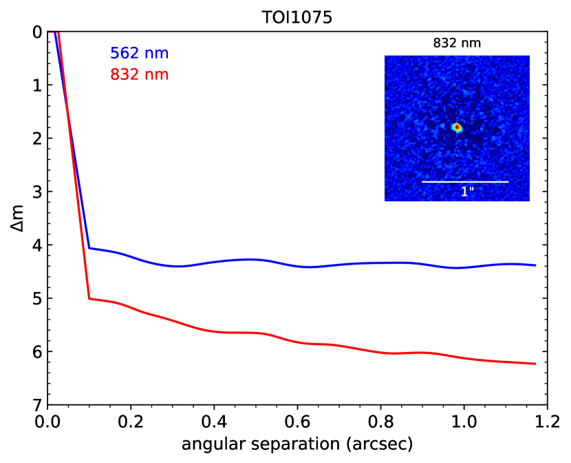
Figure 2: Gemini South Zorro contrast curves for 562 nm (blue line) and 832 nm (red line) speckle observations, and 832 nm image (inset) of TOI-1075. No visual companions are detected anywhere in Zorro’s field of view.

2.5 Stellar Kinematics and Population

Gaia Collaboration (2022k) provides the most accurate position and proper motion for TOI-1075 (=Gaia DR3 6426188308031756288) and Bailer-Jones et al. (2021) converts the Gaia DR3 trigonmetric parallax ($\varpi=16.282\pm 0.013$ mas) into a geometric distance of $d=61.43^{+0.18}_{-0.67}$ pc. Gaia Collaboration et al. (2018) lists a median radial velocity of $v_{r}$ = $31.07\pm 0.30$ km s^-1  averaged over 24 epochs. Using formulae from ESA (1997), we convert the Gaia DR3 astrometry and radial velocity into Galactic barycentric velocities: $U,V,W$ = 33.49, -31.58, 7.49 ($\pm$0.22, 0.30, 0.20) km s^-1 . The star’s 3D velocity is not near any of the 29 nearby young stellar groups tracked by Gagné et al. (2018), and the BANYAN $\Sigma$ tool returns membership probabilities of zero ($<$0.1%). Using the formulae and parameters from Bensby et al. (2014), we estimate Galactic population kinematic membership probabilities for TOI-1075 of P(thin disk) = 98.2%, P(thick disk) = 1.8%, P(halo) = $4.2\times 10^{-3}$%, P(Hercules) = $1.3\times 10^{-2}$%, i.e. TOI-1075 is $\sim$56$\times$ more likely to be a thin disk star than a thick disk star based on its velocity alone. The oldest thin disk stars are approximately $\sim$8-9 Gyr (e.g. Kilic et al., 2017; Fuhrmann et al., 2017; Fantin et al., 2019; Tononi et al., 2019).

We calculated the 3D separation between TOI-1075 and all the stars in the Gaia Catalogue of Nearby Stars (Gaia Collaboration et al., 2021) to search for any potential stellar companions. We find that TOI-1075 has no neighbors within 2 pc, and Gaia DR3 6429596764016919296 ($\Delta$ = 2.00 pc; component of the tight binary 2MASS 20335172-6403200) is its nearest star.

The systematic survey for common proper motion companions to stars within 100 pc by Kervella et al. (2022) did not yield any matches of TOI-1075 with any Hipparcos stars. A query of the Gaia Collaboration (2022k) catalog within 2^∘ ($\sim$2.0 pc) of TOI-1075 searching among stars with parallaxes and proper motions within 25%  of the values for TOI-1075 yielded no plausible common proper motion companions. Thus, TOI-1075 appears to be a single star.

The space velocity of TOI-1075 may provide some additional clues about its age. In the GCNS catalog of stars within 100 pc, there are 153 stars whose $UVW$ velocities are within 10 km s^-1  of TOI-1075. Thirty eight of the 153 stars are lacking SIMBAD entries and have not been noted in the literature. Among the 115 with SIMBAD entries, 60 have fiducial spectral types in SIMBAD and none are hotter than the F5V star HD 43879 ($T_{\rm eff}$  = $6566\pm 86$ K; Casagrande et al., 2011). A query of stellar parameter catalogs with mass estimates (Schofield et al., 2019; Stassun et al., 2019; Paegert et al., 2021; Reiners et al., 2022), shows that among the $d$ $<$ 100 pc stars with velocities within 10 km s^-1  of TOI-1075, there is a noticeable lack of stars more massive than 1.40 $M_{\sun}$. The list of GCNS stars with velocities within 10 km s^-1  of TOI-1075 was also queried through the compendium of chromospheric activity measurements ($\log R^{\prime}_{\rm HK}$) from Boro Saikia et al. (2018). Only 8 of the stars had $\log R^{\prime}_{\rm HK}$  measurements, and only two had $\log R^{\prime}_{\rm HK}$  $>$ -4.8 (approximately corresponding to the Sun on its very most active days; Egeland et al., 2017): the planet host star HD 128356 (HIP 71481; K2.5IV, $\log R^{\prime}_{\rm HK}$  = -4.73) and 6 And (HD 218804, HIP 114430; F5V, $\log R^{\prime}_{\rm HK}$  = -4.52). 6 And is a 2.99${}^{+0.48}_{-0.99}$ Gyr-old, fast-rotating ($v$sin$i$ = 19 km s^-1; Schröder et al., 2009) F5V star near the Kraft break, and so not unusually fast-rotating or young. The $\log R^{\prime}_{\rm HK}$  value for HD 128356 (-4.73) appears to be spurious, however, as the assumed B-V color from Hipparcos (0.685) is based on a single ground-based measurement (Mermilliod et al., 1997) which is at odds with the star’s spectral type (K3V or K2.5IV; Upgren et al., 1972; Gray et al., 2006) and the star’s $T_{\rm eff}$, for which the published estimates are in tight agreement (4932-4953 K; Sousa et al., 2018; Luck, 2018; Soto & Jenkins, 2018). Adopting the B-V estimate for HD 128356 from the Tycho catalog ($1.04\pm 0.02$ mag), which is more consistent with that for a K3 dwarf star, the median Mt. Wilson S-value quoted by Boro Saikia et al. (2018, S=0.214) translates (via formulae from Noyes et al., 1984) to a more benign chromospheric activity level of $\log R^{\prime}_{\rm HK}$  = -5.06. Hence, the stars that have 3D velocities within 10 km s^-1  of TOI-1075 that are Sun-like (excluding the mid-F star 6 And) with Ca H & K indices all have $\log R^{\prime}_{\rm HK}$  $<$ -4.8, consistent with ages of $\gtrsim$3 Gyr (Mamajek & Hillenbrand, 2008).

We conclude that the lack of $>$1.40 $M_{\sun}$  stars with similar velocities to TOI-1075 suggests that stars with similar orbits are unlikely to be $\lesssim$2 Gyr, and the small number of stars with published chromospheric activity indices seem to tell a similar story (lacking in stars $\lesssim$3 Gyr). It appears that stars younger than $\lesssim$2 Gyr have not yet scattered into the velocity space adjacent to the orbit of TOI-1075, suggesting that the star is either a middle-aged or old thin disk star, likely with an age between 2-9 Gyr.

2.6 Metallicity

TOI-1075 was spectrally characterized by the RAVE (RAVE J203953.3-652658, Kordopatis et al., 2013; Kunder et al., 2017; Steinmetz et al., 2020) and GALAH (Buder et al., 2018, 2021) stellar spectroscopy surveys, from which wildly disparate metallicity estimates have been published, ranging from [M/H] = $-0.99\pm 0.09$ (Kunder et al., 2017) to [Fe/H] = $0.38\pm 0.07$ (Buder et al., 2021).

An independent photometric estimate of the metallicity can be made based on the star’s position on a color-magnitude diagram. Using the $V-K_{s}$ vs. $M_{Ks}$ calibration from Johnson & Apps (2009) and Schlaufman & Laughlin (2010), we find that the color-mag position for TOI-1075 ($V-K_{s}$ = 3.584, $M_{Ks}$ = 5.176) is only 0.056 mag below the mean main sequence for late K- and M-dwarfs, translating to photometric metallicity estimates of [Fe/H] = -0.08 (Johnson & Apps, 2009) and -0.21 (Schlaufman & Laughlin, 2010). A similar estimate can be done using 2MASS and Gaia photometry by interpolating the photometry and metallicities of nearby M-dwarfs in Mann et al. (2015). As with $V-K_{s}$ vs. $M_{Ks}$, the star sits slightly below the Solar-metallicity sequence in $M_{G}$ using $B_{P}-R_{P}$, $J-K$, or $G-K_{S}$. This interpolation method gave us a metallicity estimate of [Fe/H] = -0.10$\pm$0.12, consistent with the first estimate from Johnson & Apps (2009).

We also analyzed the iodine-free PFS template spectrum using the publicly available code SpecMatch-Emp (Yee et al., 2017). This code matches a target spectrum with a library of observed spectra from stars with empirically determined stellar properties, and is particularly well-suited for the analysis of late-type stars. We recovered $T_{\rm eff}=3824\pm 70$ K, $R_{\star}=0.57\pm 0.06~{}R_{\odot}$, and $\mathrm{[Fe/H]}=-0.08\pm 0.09$ dex. The SpecMatch-Emp recovered metallicity thus corroborates the photometric metallicity measurement.

2.7 Stellar Variability

WASP-South, an array of 8 cameras composed of Canon 200-mm, f/1.8 lenses backed by 2k$\times$2k CCDs, was the Southern station of the WASP transit-search survey (Pollacco et al., 2006). The field of TOI-1075 was observed every year from 2008 to 2012, covering spans of 100 d to 180 d in each year. Within each night the cadence was typically 15-min, accumulating a total of 38 000 data points. TOI-1075 is the only bright star in the 48″  photometric extraction aperture. We searched the WASP data for a rotational modulation using the methods described in Maxted et al. (2011) but we find no significant modulation for any period between 1 and 100 days. Within each season the 95%-confidence upper limit on the amplitude is 3 mmag. Combining all the years of data results in an upper limit of 1.6 mmag. The periodograms of each season of WASP-South data showing no significant rotation modulation are shown in Figure 3. The peaks near 30 days are compatible with the residual effects of moonlight propagating through the pipeline at a low level, and thus are unlikely to be caused by TOI-1075. The lack of any rotational modulation is unusual for a cool star. McQuillan et al. (2014) report that 83% of stars cooler than 4000 K in the Kepler field show a rotational modulation, with most having amplitudes in the range 3–10 mmag. Hence TOI-1075 is among the least photometrically variable $\sim$ 20% of stars of its spectral type. TOI-1075’s low levels of stellar variability support the finding that the star is at least 2 Gyr old.

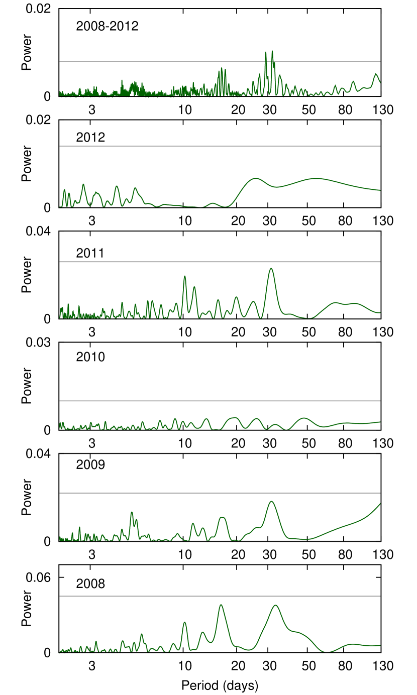
Figure 3: Periodograms of each season of WASP data for TOI-1075, showing the absence of any significant rotational modulation. The horizontal lines mark the 95%-confidence false-alarm level. The top panel is the periodogram for the 5 years of data combined.

3 Exoplanet Detection & Follow Up

3.1 TESS Time Series Photometry

The TESS primary mission surveyed the northern and southern ecliptic hemispheres in sectors measuring 24${}^{\circ}\times$ 96^∘, with near-continuous photometric coverage over $\sim$27 days. The TESS Primary Mission ran for 2 years (July 2018 – July 2020), and consisted of 26 sectors. TESS began its first extended mission in July 2020 which will end in September 2022 (when the second extended mission is scheduled to commence), and consists of 29 sectors. TOI-1075 (TIC 351601843, 2MASS J20395334-6526579) was selected for transit detection observations by TESS with 2-minute cadence as part of the Candidate Target List (CTL) – a pre-selected target list prioritized for the detection of small planets (Stassun et al., 2018, 2019). TOI-1075 was observed by TESS in Sector 13 from UT 2019 June 19 through 2019 July 18 during the primary mission, and again from UT 2020 July 4 through 2020 July 30 in Sector 27 during the first TESS Extended Mission. The star fell on Camera 2 in both sectors.

The raw TESS data for TOI-1075 were processed with the Science Processing Operations Center Pipeline (SPOC; Jenkins et al., 2016) – which performs pixel calibration, light curve extraction, de-blending from nearby stars, and removal of common-mode systematic errors – and are available at the Mikulski Archive for Space Telescopes (MAST) website. The SPOC data include both simple aperture photometry (SAP) flux measurements (Twicken et al., 2010; Morris et al., 2017) and presearch data conditioned simple aperture photometry (PDCSAP) flux measurements (Smith et al., 2012; Stumpe et al., 2012, 2014). The instrumental variations present in the SAP flux are removed in the PDCSAP flux data.

We further detrended the TESS PDCSAP data by median normalizing, flattening, fitting a low order spline, and removing 3-$\sigma$ outliers from each sector’s flux measurements separately, before stitching the light curves together. The detrended TESS PDSCAP data for Sector 13 and Sector 27, as well as the phase-folded light curve are shown in Figure 4.

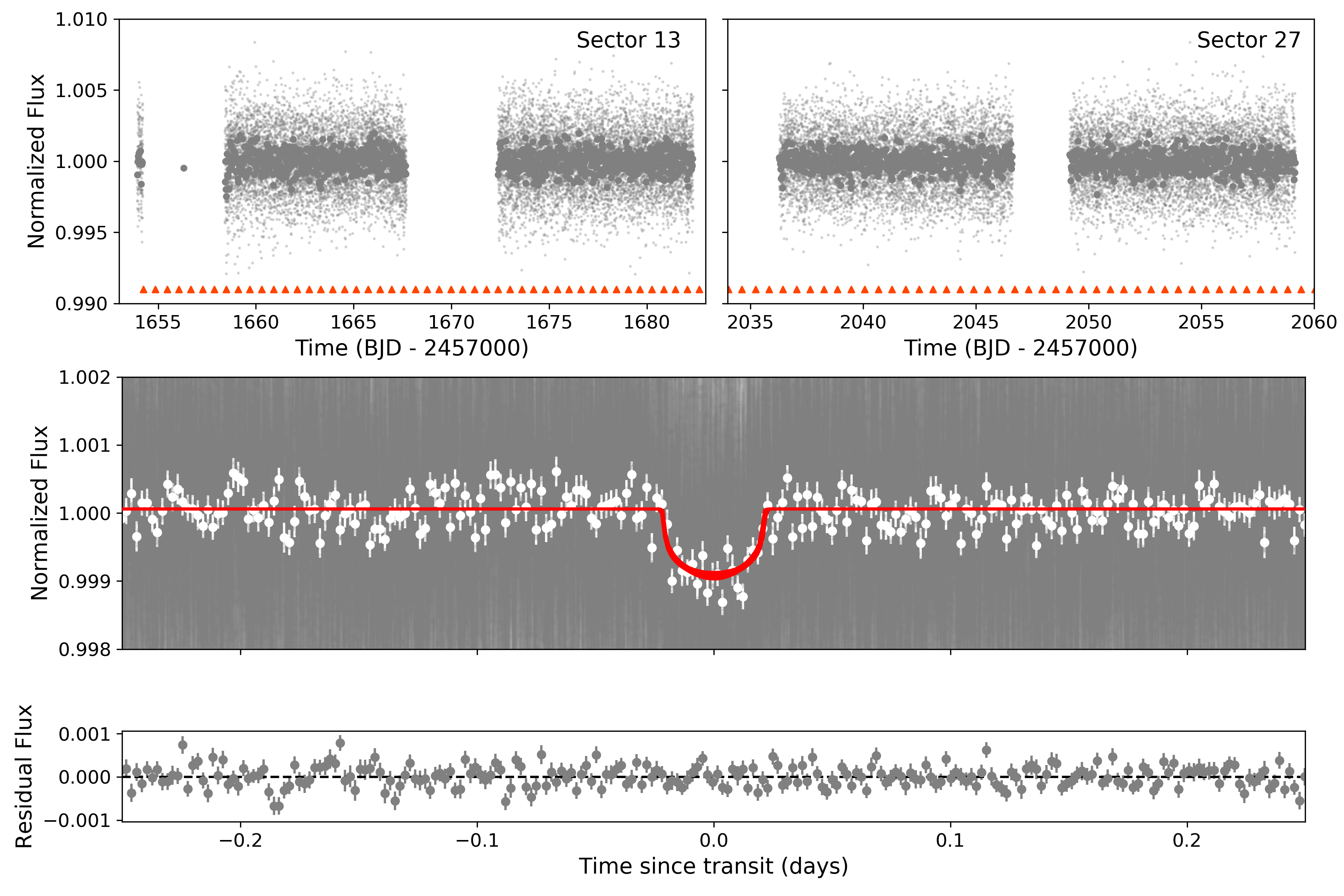
Figure 4: TESS light curves of TOI-1075. Top: Detrended, normalized and flattened PDCSAP flux measurements for Sector 13 (left) and Sector 27 (right). Lighter gray points are the TESS 2-minute cadence flux measurements; darker points are the same data binned into 30-minute intervals. The transits of TOI-1075 b are marked by orange triangles. Middle: Phase-folded light curve on planet’s orbital period (0.605 days), along with the best-fit transit model (red). Gray points are 2-minute cadence measurements; white points are the same data binned into 5-minute intervals. Bottom: Residuals after the data have been subtracted from the best-fit model.

3.1.1 TESS Transit Detection

The SPOC Transiting Planet Search (TPS; Jenkins, 2002; Jenkins et al., 2010) pipeline searches for threshold crossing events (TCEs) in the PDCSAP light curve, applying an adaptive noise-compensating matched filter to account for stellar variability and residual observation noise. TCEs with a period of 0.605 days were detected independently in the SPOC transit search of the Sector 13 light curve, Sector 27 light curve, and multisector light curves from Sectors 13 and 27.

In order to rule out false positives that can mimic the planetary transit signal, we evaluated the star’s data validation reports (DVR; Twicken et al., 2018; Li et al., 2019), which are generated from the SPOC 2-minute cadence data. The multisector DVR shows no evidence of secondary eclipses, odd/even transit depth inconsistencies, or correlations between the depth of the transit and the size of the aperture used to extract the light curve – which would indicate that the transit signal originated from a nearby eclipsing binary. Additionally, the location of the transit source as shown in the DVR is consistent with the position of the target star – the difference image centroiding test located the source of the transits due to TOI-1075 b to within $1.64\pm 4.69$” of TOI-1075, which complements the speckle imaging observations. Upon passing these vetting checks, the transit signal was assigned the identifier TOI-1075.01 and announced by the TESS TOI team. (Guerrero et al., 2021).

3.2 Ground-based Time-Series Photometry

After it was alerted as a TOI, we acquired ground-based time-series follow-up photometry of TOI-1075 during future times of transit predicted by the TESS data. We used the TESS Transit Finder, which is a customized version of the Tapir software package (Jensen, 2013), to schedule our transit observations.

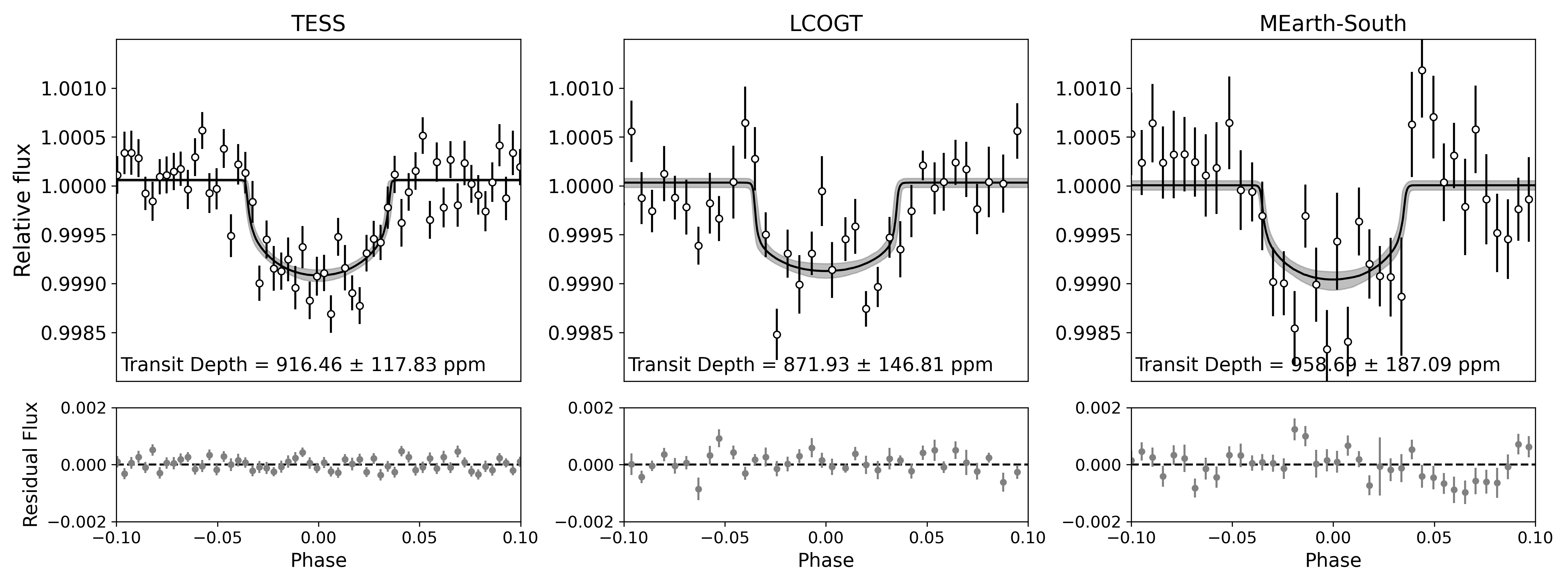
Figure 5: Results of the juliet joint fit to the TESS photometry, and ground-based LCOGT and MEarth-South photometry. Top: Transit observations of the respective instruments phase-folded to the period of TOI-1075 b. The black curve is the best-fit juliet transit model, and the 68% confidence interval is represented by the gray shaded region. The binned data points with errorbars are shown for clarity (white circles). The TESS data are binned in 2-minute intervals, and the LCOGT and MEarth-South data are binned in 5-minute intervals. Bottom: Residuals after the data have been subtracted from the best-fit model.

3.2.1 LCOGT 1 m Observations

We observed five full transits of TOI-1075 in Pan-STARRS $z$-short band from the Las Cumbres Observatory Global Telescope (LCOGT; Brown et al., 2013) 1.0 m network on UTC 2019 August 25, 2019 August 26, 2019 September 23, 2019 September 24, and 2019 September 26 (Figure 5). The first, third and fifth observations were conducted from the South African Astronomical Observatory (SAAO) node, and the second and fourth observations from the Siding Spring Observatory(SSO) node. The 1 m telescopes are equipped with $4096\times 4096$ SINISTRO cameras having an image scale of $0\farcs 389$ per pixel, resulting in a $26\arcmin\times 26\arcmin$ field of view. The images were calibrated by the standard LCOGT BANZAI pipeline (McCully et al., 2018). Photometric data were extracted using AstroImageJ (Collins et al., 2017) and circular photometric apertures with radii in the range $6\farcs 2$ to $7\farcs 8$. The target star apertures exclude flux from all known nearby Gaia DR3 and TESS Input Catalog stars. We detect the event on-target in all five data sets, which are included in the joint model of the system in this work.

3.2.2 MEarth-South 0.4m Observations

We observed two full transits of TOI-1075 b using the MEarth-South telescope array (Nutzman & Charbonneau, 2008; Irwin et al., 2015) at Cerro Tololo Inter-American Observatory (CTIO), Chile on UT 2019 September 22 and 2019 September 28 (Figure 5). Observations were gathered for approximately 5.5 hours centered on the predicted time of mid-transit. The data were reduced using the standard MEarth processing pipeline (e.g. Berta et al. 2012) with a photometric extraction aperture of $r=14$ pixels (11.8″). Twelve light curves were observed across 6 telescopes, and were collected with an RG715 filter. All of the light curves contain meridian flips prior to the predicted time of ingress. These were accounted for in the analysis of the light curves by allowing for separate magnitude zero points for each combination of telescope and side of the meridian to remove any residual flat fielding error. Some residuals in the out of transit baseline, likely due to color-dependent atmospheric extinction, were found so the final model also included a linear decorrelation against airmass.

3.2.3 Previous Validation of TOI-1075 b

Additionally, planet candidate TOI-1075.01 was statistically validated as a planet using TESS and ground-based photometry in Giacalone et al. (2022). TOI-1075.01 was vetted with DAVE (Kostov et al., 2019) which uses centroid offset analyses to identify evidence of false positives due to contamination from nearby stars, and with TRICERATOPS (Giacalone & Dressing, 2020; Giacalone et al., 2021), which calculates the Bayesian probability that the candidate is an astrophysical false positive. TOI-1075.01 showed no strong indicators of being a false positive in the aforementioned analysis, and was then validated as TOI-1075 b (Giacalone et al., 2022).

3.3 Time Series Radial Velocities

We collected 18 precision radial velocity epochs of TOI-1075 using the Planet Finder Spectrograph (PFS; Crane et al., 2006, 2008, 2010) on the 6.5 m Magellan II (Clay) telescope at Las Campanas Observatory in Chile. PFS is a slit-fed spectrograph that is wavelength calibrated using an iodine cell, and covers the wavelength range $391-734$ nm, though only the 500-620 nm range is used when measuring RV shifts. All PFS spectra are reduced and RVs extracted using a custom IDL pipeline based on Butler et al. (1996) that regularly delivers sub-1 m s^-1 precision. Each of the 18 PFS TOI-1075 iodine observations consist of 3$\times$20-minute exposures, and were mostly obtained on a night-by-night basis between UT 2021 May 22 and UT 2021 November 15, although in some cases two observations were taken on the same night but separated in time by at least 1-2 hours. A two-hour, iodine-free template observation was obtained on UT 2021 May 29. All observations were taken with the default 0.3$\arcsec$ slit but in 3$\times$3 binning mode, resulting in a resolving power of R$\sim$110,000. The resulting unbinned (20-minute integration time) RVs have typical precisions of 2.5–3.0 m s^-1, and are listed in full in Table LABEL:tab:RVs.

A generalized Lomb–Scargle (GLS) periodogram of the PFS RV data shows a significant peak at 0.605 days (Figure 6), which matches the orbital period of the planet candidate determined from the TESS data. An additional significant peak at $\sim$15 days likely corresponds to a stellar activity signal. The stellar activity signal is well-separated from the planet period, and there are no stellar periodicity signals more dominant than the planet signal, nor any significant stellar signals that appear around the planet period. Additionally, we modeled the suggested stellar activity signal using a Gaussian Process (GP) and find no evidence to incorporate it into our final model (see Section 4.2.1). Therefore, incorporating GPs for non-white noise models, or adding another term to our RV model fit was deemed unnecessary.

Table 2: PFS RV data of TOI-1075

Date (BJDTDB)	RV ($\rm m\,s^{-1}$)	$\sigma_{RV}$ ($\rm m\,s^{-1}$)
2459356.868	-12.48	2.90
2459356.884	-5.77	3.04
2459356.897	-14.11	2.65
2459357.856	-25.83	3.00
2459357.870	-8.09	2.52
2459357.885	-18.11	3.38
2459358.848	-30.56	2.40
2459358.862	-26.80	2.18
2459358.876	-27.47	2.30
2459452.564	-11.29	2.34
2459452.578	-11.31	2.49
2459452.593	-6.06	2.57
2459452.665	-12.61	2.69
2459452.679	-5.05	2.56
2459452.693	-6.42	3.01
2459470.617	10.02	3.18
2459470.631	-6.18	3.05
2459470.645	1.55	3.65
2459471.561	10.02	2.61
2459471.576	14.14	2.58
2459471.590	13.93	2.55
2459471.659	15.38	2.71
2459471.673	13.14	2.52
2459471.687	6.22	2.58
2459473.537	11.41	2.48
2459473.550	17.32	2.52
2459473.565	20.98	3.25
2459473.647	6.82	3.02
2459473.661	10.98	3.19
2459473.675	14.55	3.39
2459474.554	-3.83	2.69
2459474.568	4.77	2.62
2459474.583	-2.40	3.05
2459474.616	6.56	3.00
2459474.630	2.55	3.02
2459475.526	-5.85	3.07
2459475.540	-3.90	2.47
2459475.554	-6.89	2.60
2459501.537	7.60	2.90
2459501.551	-2.56	2.80
2459501.565	4.48	2.86
2459504.528	0.00	2.47
2459504.542	-9.94	2.75
2459504.556	-12.43	2.91
2459505.549	11.69	4.34
2459505.563	7.41	3.99
2459505.578	4.74	3.25
2459506.518	-19.93	2.41
2459506.532	-1.76	2.45
2459506.546	-14.89	2.33
2459531.523	7.30	2.49
2459531.537	10.63	2.55
2459533.536	7.42	2.67
2459533.546	11.35	4.27

Figure 6: Generalized Lomb–Scargle periodogram of the radial velocity measurements from PFS. There is a clear peak at the period of TOI-1075 b (gray bar). We identify a stellar activity signal at $\sim$15 days (red dashed line) which is well-separated from TOI-1075 b’s orbital period.

4 System Parameters from juliet

To obtain precise parameters of the TOI-1075 system, we performed a joint analysis of the TESS, LCOGT, and MEarth-South photometry, and the PFS RV data using juliet (Espinoza et al., 2019). juliet is a fitting tool that uses nested sampling algorithms to efficiently sample a given parameter space, and allows for model comparison based on Bayesian evidences. juliet combines the publicly available packages for transits and RV modeling, batman (Kreidberg, 2015) and radvel (Fulton et al., 2018), respectively. We opted to implement dynesty (Speagle, 2020) as the nested sampling algorithm for our joint fitting, though a range of nested sampling algorithms are available to choose from.

4.1 Transit Modeling

For the transit modeling, juliet employs the batman package. We adopt a quadratic model to describe the limb darkening effect in the TESS, LCOGT, and MEarth-South photometry, and parameterize it by employing the efficient, uninformative sampling scheme of Kipping (2013), and a quadratic law. We used a fixed dilution factor of 1 for all instruments, but considered free individual instrumental offsets. Instrumental jitter terms were taken into account and added in quadrature to the nominal instrumental errorbars. We used uniform priors per the Espinoza (2018) parameterization to explore the full physically plausible parameter space for the planet-to-star radius ratio, $p=R_{p}/R_{\star}$, and impact parameter, $b$. Additionally, we defined a log-uniform prior on the stellar density, and then recovered the scaled semi-major axis ($a/R_{*}$) using Kepler’s third law.

4.2 RV Modeling

The model that we selected for our RV joint fit analysis was composed of a circular Keplerian orbit for the transiting planet (ultra-short period planets are expected to be tidally circularized), and an additional linear long-term trend to constrain the non-Keplarian long-period signal present in the PFS RV data, whose period is longer than the current observation baseline. We assumed uniform wide priors for the systemic velocity, jitter term, and RV semi-amplitude of the PFS RVs, as well as the linear long-term trend parametrized by an intercept $B$, and a slope $A$. We measured a radial velocity semi-amplitude of $K=10.95^{+1.50}_{-1.43}~{}\rm m\,s^{-1}$ for TOI-1075 b.

4.2.1 RV Model Comparison

juliet searches for the global posterior maximum based on the evaluation of the Bayesian log-evidence ($\ln\mathcal{Z}$), allowing us to perform model comparisons given the differences in $\Delta\ln\mathcal{Z}$. We modeled the PFS RV data with and without fitting a linear long-term trend to the data. The model with the linear long-term trend had a log-evidence of $\ln\mathcal{Z}$ = $-$204.01 $\pm$ 0.38, and the model without the linear long-term trend (a circular Keplarian model only) had a log-evidence of $\ln\mathcal{Z}$ = $-$212.95 $\pm$ 0.28, resulting in a $\Delta\ln\mathcal{Z}$ = 8.94. We selected the model with the linear long-term trend component following criteria described in Trotta (2008), which considers a $\Delta\ln\mathcal{Z}$ $>$ 2 as weak evidence that one model is preferred over the other, and a $\Delta\ln\mathcal{Z}$ $>$ 5 as strong evidence that one model is significantly preferred over the other, hence the additional model parameters are necessary to account for the long-period signal in the PFS RV data. We also considered a model composed of a circular Keplerian orbit, and a long-term trend parametrized by an intercept $B$, a slope $A$, and a quadractic/curvature coefficient, $Q$. The change in log-evidence was $\Delta\ln\mathcal{Z}$ $<$ 2 between the long-term trend parametrization with and without the additional parameter, $Q$, confirming that the RV data are legitimately fitted by a circular Keplerian model and a linear long-term trend. As an additional test, we added a stellar signal to the RV model using a GP to determine the effect of the 15-day period signal identified in the PFS GLS periodogram (Figure 6). We compared the models with and without the additional stellar signal and found no evidence ($\Delta\ln\mathcal{Z}$ $<$ 2) that the final model required the addition of a stellar signal.

We show the final transit and RV models of the joint fit based on the posterior sampling in Figures 5 and 7 respectively, the posterior parameters of our joint fit in Table LABEL:tab:julietposteriors, the selected priors for our joint fit in Table LABEL:tab:julietpriors, the obtained posterior probabilities in Figure A1, and the derived planetary parameters of TOI-1075 b based on the posteriors of the joint fit in Table LABEL:tab:julietderived.

To summarize, the TOI-1075 system consists of a late K-/early M-dwarf host star with at least one hot super-Earth planet, TOI-1075 b (see Table LABEL:tab:julietderived), which has a mass of $M_{p}$ = 9.95${}^{+1.36}_{-1.30}$ $M_{\earth}$ and radius of $R_{p}$ = 1.791${}^{+0.116}_{-0.081}$ $R_{\earth}$  on a circular orbit with a period of 0.605 days. We derived a bulk density of $\rho$ = $9.32^{+2.05}_{-1.85}$ g cm^-3 and an equilibrium temperature, assuming a zero albedo, of $T_{eq}=1323\pm 44$ K.

Figure 7: Results of the juliet joint fit to the PFS radial velocities. Top: PFS RVs over time (black points), and full best-fit juliet model (gray curve). Middle: Phase-folded RV measurements from PFS. The black curve is the best-fit juliet RV model, the gray points are the unbinned RVs, and the red diamonds are the RV measurements binned in 0.05 units of orbital phase. Errorbars are the quadrature sum of the PFS internal uncertainties, and the RV jitter estimate from the juliet fit.The best-fit RV semi-amplitude is $K=10.95^{+1.50}_{-1.43}~{}\rm m\,s^{-1}$. Bottom: RV residuals after the data have been subtracted from the best-fit model.

5 Discussion

Our RV measurements of TOI-1075 b constrain the planetary mass with an uncertainty of $\sim 14$%, and the TESS, LCOGT and MEarth-South light curves constrain the planetary radius with an uncertainty of $\sim 7$%. Thus, TOI-1075 b belongs to the small group of super-Earths with precisely measured masses and radii, or those planets with measurement precision better than 30% (see Figure 8). With precise mass and radius measurements in hand for TOI-1075 b, we discuss implications for radius valley studies, the potential for planetary atmospheric characterization, potential planetary compositions, planetary bulk density, and possible planet formation mechanisms. We also discuss constraints on a potential second planet in the TOI-1075 system.

5.1 Implications for the Radius Valley around M-dwarfs

Several physical mechanisms/theoretical models have been proposed to explain the existence of the radius gap. These mechanisms include thermally driven atmospheric mass loss, e.g., photoevaporation (Lopez et al., 2012; Chen & Rogers, 2016; Owen & Wu, 2017) and core-powered mass loss (Ginzburg et al., 2018; Gupta & Schlichting, 2019, 2020); and gas-poor formation – a natural outcome of planet formation, where rocky super-Earths are a result of formation in gas-poor environments, without requiring any atmospheric escape (Lee et al., 2014; Lee & Chiang, 2016; Lopez & Rice, 2018; Lee & Connors, 2021). The slope of the radius valley (in period-radius space) can be used to discern between a thermally driven mass-loss model or a gas-poor formation model (Lopez & Rice, 2018; Gupta & Schlichting, 2020; Lee & Connors, 2021).

The slope of the radius valley around Sun-like stars has been characterized using data from the Kepler and K2 missions, and both thermally driven mass-loss and gas-poor formation models are favored in this stellar-mass regime (Van Eylen et al., 2018; Martinez et al., 2019). However, around low-mass mid-K- to mid-M-dwarfs, Cloutier & Menou (2020) found tentative evidence that the slope of the radius valley is consistent with predictions from gas-poor formation. Additionally, the radius gap decreases as stellar radius decreases, and the radius gap is centered at $1.54\pm 0.16$ R_⊕ for low-mass K- and M-dwarf stars (vs. 1.75 R_⊕ for Sun-like stars in Fulton et al. 2017).

TOI-1075 b lies between the predicted slopes of the thermally driven mass loss model and gas-poor formation model, and hence within the M-dwarf radius valley created by these mechanisms (the M-dwarf radius valley ranges from 1.5-2.5 R_⊕ between the predicted slopes – see Figure 9 in Cloutier et al., 2021). TOI-1075 b’s orbital period (0.605 days) and size (1.791${}^{+0.116}_{-0.081}$ $R_{\earth}$) make it a “keystone planet” – a valuable target to conduct tests of competing radius valley models across a range of stellar masses, using precise planetary mass and radius measurements (Cloutier & Menou, 2020). TOI-1075 b joins TOI-1235 b (Cloutier et al., 2020; Bluhm et al., 2020), TOI-776 b (Luque et al., 2021), TOI-1685 b (Bluhm et al., 2021), and TOI-1634 b (Cloutier et al., 2021) as keystone planets that will help elucidate the physical mechanism that formed the radius valley around early M-dwarfs. Distinguishing between the two atmospheric loss mechanisms will require the discovery of additional keystone planets for statistical studies and population analysis, as well as atmospheric studies of TOI-1075 b and other keystone planets to provide observational evidence to validate model predictions.

5.2 Atmospheric Characterization Prospects

Super-Earths with $R_{p}>$ 1.6 R_⊕ are expected to have a substantial H/He atmosphere (Rogers, 2015), and though TOI-1075 b’s radius (1.791${}^{+0.116}_{-0.081}$ $R_{\earth}$) places it just above the radius gap, its bulk density is inconsistent with the presence of a low mean-molecular weight envelope. Based on TOI-1075 b’s predicted composition (see Section 5.3) and ultra-short orbital period, we do not expect the planet to have retained a H/He envelope. But, TOI-1075 b could either have: no atmosphere (bare rock); a metal/silicate vapor atmosphere with a composition set by the vaporizing magma-ocean on the surface (Schaefer & Fegley, 2009; Ito et al., 2015) since TOI-1075 b’s equilibrium temperature is hot enough to melt a rocky surface (Mansfield et al., 2019); or, especially at the low-end of its allowed mean density range, possibly a thin H/He or CO₂ or other atmosphere. A detailed atmospheric model is needed to determine possible atmospheric compositions for TOI-1075 b, which is beyond the scope of this work.

We calculated the emission spectroscopy metric (ESM) and transmission spectroscopy metric (TSM), as defined by Kempton et al. (2018), to determine TOI-1075 b’s potential for atmospheric characterization. Using the stellar parameters reported in Section 2.2, and the planetary parameters in Table LABEL:tab:julietderived, we obtain ESM $=10.1\pm 1.6$ and TSM $=29\pm 8$.

TOI-1075 b is a good candidate for emission spectroscopy with the James Webb Space Telescope (JWST). The planet may have a mineral-rich atmosphere consisting of metal and silicate vapors, since its equilibrium temperature is high enough to melt silicate rock (Schaefer & Fegley, 2009; Léger et al., 2011; Ito et al., 2015; Ito & Ikoma, 2021). If TOI-1075 b has no atmosphere, its surface may be characterized via secondary eclipse observations. With an ESM value of $10.1\pm 1.6$, TOI-1075 b is well above the threshold ESM of 7.5 suggested by Kempton et al. (2018) for a high-quality atmospheric characterization target. TOI-1075 b is one of only 8 super-Earths: 55 Cancri e (Bourrier et al., 2018), HD 213885 b (Espinoza et al., 2020), HD 3167 b (Christiansen et al., 2017), TOI-431 b (Osborn et al., 2021), TOI-500 b (Serrano et al., 2022), TOI-1807 b (Nardiello et al., 2022) and K2-141 b (Malavolta et al., 2018), with mass measurement precision $>5\sigma$ and with V/J/H/K $<$ 13 mag, that has an ESM $>$ 7.5. It is also the only super-Earth above the radius gap in the temperature range 1250–1750 K, which will allow us to probe an intermediate temperature range of hot super-Earths and explore the atmospheric species that have volatilized in this regime.

In addition to having an ESM value above the suggested threshold, TOI-1075 b can also be observed by JWST for $\sim 200$ days per year. Thus, TOI-1075 b is accessible to JWST for a significant portion of the year, which allows for more flexibility when planning observations.

Kempton et al. (2018) suggests that TSM $>90$ be used as the threshold for planets with 1.5 R_⊕ $<$ R_p $<$ 10 R_⊕. TOI-1075 b does not meet this criteria because, due to its high mass and hence high surface gravity, it is unlikely to have an extended atmosphere that can be probed in transmission.

5.3 Planetary Composition and Density

The measured mass and radius of TOI-1075 b result in a planetary bulk density of $9.32^{+2.05}_{-1.85}$ g cm^-3, which is almost twice as dense as the Earth ($\rho_{\earth}$ = 5.51 g cm^-3). Comparing TOI-1075 b with the theoretical composition models of Zeng et al. (2021) and Lin et al. (in prep), the planet’s bulk density is consistent with a 35% Fe + 65% silicates by mass composition (see Figure 8).

To simulate TOI-1075 b’s interior, we numerically integrate three equations – the mass of a spherical shell, hydrostatic equilibrium, and the equation of state (EOS) – from the planet’s center to the surface with a step size of 100 m using a planetary interior simulation code (Lin et al. (in prep)). The code is validated against recent mass-radius curves calculated by Zeng et al. (2021). We assume a completely differentiated planet with an iron core and a mantle consisting of silicates. For iron and silicates, we adopt a second-order adapted polynomial EOS developed by Holzapfel (2018), using EOS coefficients listed in Zeng et al. (2021). The inner boundary conditions of the simulated planets are assumed to be $M(0)=0$ and $P(0)=P_{c}$, where $P_{c}$ is the central pressure. We switch from the iron core to the silicate mantle when the desired core mass has been reached. The iteration terminates when the outer boundary condition $P(R)\leq 1$ bar is satisfied. We use a bisection method to search for the $P_{c}$ that produces $M(R)=M_{p}$ for a given core-mass fraction (CMF). Using the mean measured mass and radius of TOI-1075 b, we compute a mean CMF of $0.35$. We then calculate a core-radius fraction (CRF) by dividing the radius of the iron layer by the total radius of the planet, resulting in a mean CRF of $0.52$, or $0.93\,$R_⊕.

We further consider the most and least dense scenarios permissible by the mass and radius error bars. In the most dense scenario ($M_{p}=11.31\,$M_⊕, $R_{p}=1.709\,$R_⊕), we compute a CMF of 0.61 and a CRF of 0.67, or $1.15\,$R_⊕. In the least dense scenario ($M_{p}=8.65\,$M_⊕, $R_{p}=1.91\,$R_⊕), even a coreless pure silicates composition (CMF = 0, CRF = 0) cannot explain the low-end density of the planet. Even though such a coreless planet is unphysical from a planet formation perspective, we include this extreme scenario for completeness.

Though we have precisely measured the mass of TOI-1075 b to $>7\sigma$ (9.95${}^{+1.36}_{-1.30}$ $M_{\earth}$), the uncertainty on the mass measurement leads to a wide range of possible CMF ($0.35^{+0.26}_{-0.35}$) and CRF ($0.52^{+0.15}_{-0.52}$) values, which can only be resolved with more precise mass and radius measurements not currently available. In the following sections, we discuss possible formation scenarios that could result in the mean density, most dense, and least dense scenarios.

Figure 8: Mass–radius diagram for small planets ($R_{p}$ $<$ 2 R_⊕ and $M_{p}$ $<$ 10 M_⊕) with measured mass and radius uncertainties below 30%, as listed in the NASA Exoplanet Archive (only planet masses measured by the radial velocity method are considered). Planets are colored according to their calculated equilibrium temperature (assuming zero-albedo and efficient heat redistribution). Super-Earth planets have square symbols, and super-Mercury planets have bold diamond symbols. The gray shaded region denotes the radius gap for low-mass stars centered at $1.54\pm 0.16$ R_⊕ (Cloutier & Menou, 2020). The terrestrial solar system planets are plotted for reference. Left: Mass-radius diagram with curves of constant composition. The solid lines are theoretical internal composition curves (Zeng et al. 2021; Lin et al. (in prep)) from top to bottom: 100% H₂O (blue), 100% silicates (green), a mixture of 30% Fe and 70% silicates by mass (orange), a mixture of 50% Fe and 50% silicates by mass (light brown), a mixture of 70% Fe and 30% silicates by mass (dark brown), and 100% Fe (black). TOI-1075 b’s bulk density is consistent with a 35% Fe + 65% silicates by mass composition. Right: Mass-radius diagram with curves of constant density relative to Earth. TOI-1075 b’s density is $\sim$1.75 times greater than the Earth.

5.3.1 TOI-1075 b’s Mean Density and Composition

The mean mass and radius ($M_{p}=9.95\,$M_⊕, $R_{p}=1.791\,$R_⊕) of TOI-1075 b result in a bulk density of 9.32 g cm^-3. While TOI-1075 b’s mean bulk density is $\sim 1.75\times$ that of Earth, its mean CMF (0.35) and CRF (0.52) are consistent with a predominantly rocky, Earth-like composition and internal structure. TOI-1075 b’s uncompressed density is 4.91 g cm^-3, which is similar to the uncompressed density of the Earth (4.79 g cm^-3), further supporting our findings of an Earth-like composition for TOI-1075 b.

TOI-1075 b is the most massive and densest super-Earth with 1.6 R_⊕ $<$ R_p $<$ 2 R_⊕ discovered to date. The similarity in TOI-1075 b’s CMF relative to Earth (CMF_⊕ = 32.5%, Seager et al., 2007) supports our finding that TOI-1075 b likely lacks a massive low mean-molecular weight envelope which, if present, would have corresponded to a larger observed radius for a given mass.

A handful of massive terrestrial planets like TOI-1075 b have been discovered, but these objects are relatively rare. Planets similar in radius and Earth-like composition to TOI-1075 b are listed in Table LABEL:tab:massiveplanets.

5.3.2 TOI-1075 b As A Super-Mercury

In the most dense scenario ($M_{p}=11.31\,$M_⊕, $R_{p}=1.710\,$R_⊕, $\rho=11.37$ g cm^-3), we consider the possibility of TOI-1075 b as a super-Mercury. The term “Super-Mercuries” generally refers to planets that are super-Earth sized with enhanced uncompressed bulk densities, as compared to Earth-like planets. The high density has been interpreted to be indicative of a high iron-mass fraction, analogous to the solar system planet Mercury (Marcus et al., 2010; Adibekyan et al., 2021), and the formation mechanism for these planets is still unknown. Based on TOI-1075 b’s bulk density ($9.32^{+2.05}_{-1.85}$ g cm^-3), if the planet’s mass is at the high range, with a high core-mass fraction in the allowed range (CMF = $0.35^{+0.26}_{-0.35}$), it could be a super-Mercury. The small group of recently identified super-Mercuries include: K2-38 b, K2-106 b, K2-229 b, Kepler-107 c, and Kepler-406 b (Adibekyan et al., 2021), as well as GJ 367 b (Lam et al., 2021) and HD 137496 b (Silva et al., 2022), which are represented by bold data points in Figure 8.

We investigated possible formation mechanisms that could result in the high density, and CMF and CRF ranges observed for TOI-1075 b including: giant impacts (Marcus et al., 2010; Benz et al., 2008; Asphaug & Reufer, 2014; Liu et al., 2015; Scora et al., 2020; Cambioni et al., 2021, 2022); in-situ formation (Weidenschilling, 1978; Kruss & Wurm, 2018; Johansen & Dorn, 2022); an initially metal-rich protoplanetary disk composition (Veyette et al., 2017; Adibekyan et al., 2021; Schulze et al., 2021; Souto et al., 2022); and the decompressed core of an evaporated gas giant (Hébrard et al., 2003; Mocquet et al., 2014), but we do not have sufficient information to resolve the planet’s formation mechanism.

5.3.3 TOI-1075 b As A Low-density Planet

In the least dense scenario ($M_{p}=8.65\,$M_⊕, $R_{p}=1.907\,$R_⊕, $\rho=7.47$ g cm^-3), our interior model results in a coreless silicate planet, and requires an additional water layer to account for the inflated radius. Such a coreless planet is unphysical from a planet formation perspective – a planet with a mass of TOI-1075 b is expected to have fully differentiated e.g. Rubie et al. (2015); Cambioni et al. (2021). A water layer would be physically unstable at TOI-1075 b’s equilibrium temperature. Therefore, layers less dense than silicates must be added to the model to fit the minimum mass and maximum radius scenario. Possible candidates for these layers include low-pressure silicate phases, or a metal/silicate vapor atmosphere.

Table 3: Massive terrestrial planet parameters

Planet Name	Planet Radius ($R_{\earth}$)	Planet Mass ($M_{\earth}$)	Teq (K)	Reference
TOI-1075 b	$1.791_{-0.081}^{+0.116}$	$9.95_{-1.30}^{+1.36}$	1323$\pm 44$	This work
Kepler-20 b	${1.868}_{-0.034}^{+0.066}$	${9.70}_{-1.44}^{+1.41}$	$1105\pm 37$	Buchhave et al. (2016)
LHS 1140 b	$1.727\pm 0.032$	$6.98\pm 0.89$	$235\pm 5$	Ment et al. (2019)
TOI-1235 b	$1.738_{-0.076}^{+0.087}$	${6.91}_{-0.85}^{+0.75}$	$754\pm 18$	Cloutier et al. (2020)
HD 213885 b	$1.74\pm 0.05$	$8.8\pm 0.6$	$2128\pm 14$	Espinoza et al. (2020)
WASP-47 e	$1.808\pm 0.026$	$6.77\pm 0.57$	$2514\pm 70$	Bryant & Bayliss (2022)
K2-216 b	$1.72\pm 0.06$	$8.18\pm 1.65$	$1217\pm 34$	Clark et al. (2022)

5.4 A Potential Second Planet in the System

We find a linear long-term trend in the PFS RV data (see Section 4.2) whose period is longer than the baseline of our RV observations. This may indicate the presence of a second planet in the system. We place lower limits on the period, semi-amplitude, and mass of a second planet candidate as the source of the long-term trend.

The orbital period of the second planet candidate is at least twice the observing baseline of the PFS RV observations (otherwise we would have seen the RV trend turn over before our observations concluded as the potential planet passed through its quadrature phase). The PFS observations were taken over a period of $176.68$ days (T_baseline), hence the orbital period of the planet candidate should be at least $353$ days.

Taking the best-fit linear trend results from juliet, the RV data is shifted $0.130^{+0.017}_{-0.018}~{}\rm m\,s^{-1}\,day^{-1}$. Thus, the RV semi-amplitude of the planet candidate must be at least (T_baseline $\times$ RV Trend)/2 = $11.48~{}\rm m\,s^{-1}$.

Combining the minimum orbital period ($353$ days) and the minimum RV semi-amplitude ($11.48~{}\rm m\,s^{-1}$), and assuming a circular Keplarian orbit, the minimum mass of the second planet candidate is $\sim 87~{}M_{\earth}$ or $\sim 0.28~{}M_{\rm Jupiter}$.

The presence of a second planet candidate motivates us to collect additional RV data for this system in order to determine the period and measure the mass of the second planet candidate, while also improving the uncertainty on the mass measurement of TOI-1075 b. Additionally, there are currently a handful of systems consisting of a USP planet and a close-in companion, with periods ranging from a few days to tens of days e.g. K2-106 (Guenther et al., 2017), K2-141 (Malavolta et al., 2018), K2-229 (Santerne et al., 2018), TOI-500 (Serrano et al., 2022). These close-in companions could be responsible for migrating the USP planets to their current positions (Pu & Lai, 2019; Millholland & Spalding, 2020; Serrano et al., 2022). The possible existence of such a close-in companion in the TOI-1075 system serves as additional motivation for further RV follow-up of the system.

Determining the source of the long-term trend, and more accurately measuring TOI-1075 b’s planet mass and parameters will further detailed planet formation, planet migration and atmospheric characterization efforts, since a planet’s gravity plays an important role in its collisional history and interpreting atmospheric spectra (Batalha et al., 2019).

6 Conclusions

We report the discovery and confirmation of TOI-1075 b, a transiting, ultra-short period, hot super-Earth orbiting a nearby ($d$ = 61.4 pc) late K-/early M-dwarf star. Using photometric observations from TESS, LCOGT, and MEarth-South, and radial velocity observations from PFS, we precisely measure the radius and mass of TOI-1075 b to be 1.791${}^{+0.116}_{-0.081}$ $R_{\earth}$ and 9.95${}^{+1.36}_{-1.30}$ $M_{\earth}$, respectively. Our PFS radial velocity data also suggest the presence of a second planet candidate in the system, with a minimum mass of $\sim 87~{}M_{\earth}$ and a minimum orbital period of $\sim 353$ days. TOI-1075 b has a bulk density of $9.32^{+2.05}_{-1.85}$ g cm^-3, consistent with a composition of 35% iron by mass, and a core-radius fraction of 52%. TOI-1075 b is a good candidate for emission spectroscopy with JWST, which we can use to characterize a potentially mineral-rich atmosphere. TESS is scheduled to observe TOI-1075 again in Year 5, Sector 67 (July 2023), which will provide a more precise planet radius, and the ability to search for variations in the planet period on a 4-year timescale. TOI-1075 b is a massive, dense, high temperature, ultra-short period super-Earth inside of the M-dwarf radius valley, making the system ideal for testing planet formation and evolution theories, density enhancing mechanisms, and theoretical models related to atmospheric loss.

Table 4: Median values and 68% confidence interval for posterior parameters from joint photometric and radial velocity juliet analysis for the TOI-1075 system.

Parameter	Units	Values
Stellar Parameters:
$\rho_{*}$	Density (g cm-3)	$3.73^{+0.99}_{-1.67}$
Planet Parameters:		TOI-1075 b
$P$	Period (days)	$0.6047328\pm 0.0000032$
$T_{0}$	Time of transit center ($\rm{BJD_{TDB}}$)	$2458654.2510^{+0.00040}_{-0.00050}$
$r_{1}$	Parametrization of Espinoza (2018) for $b$	$0.60^{+0.20}_{-0.17}$
$r_{2}$	Parametrization of Espinoza (2018) for $R_{p}/R_{*}$	$0.0282^{+0.0019}_{-0.0013}$
$K$	RV semi-amplitude ($\rm m\,s^{-1}$)	$10.95^{+1.50}_{-1.43}$
$e$	Eccentricity (fixed)	$0.00$
Photometry Parameters:
		MEarth-South	LCOGT	TESS
$M$	Relative flux offset	$0.0000$	$0.0000$	$-0.0001$
$\sigma$	Jitter term for light curve (ppm)	$901.29^{+86.80}_{-91.69}$	$471.24^{+58.31}_{-62.17}$	$3.21^{+25.84}_{-2.86}$
$q_{1}$	Quadratic limb-darkening parametrization (Kipping, 2013)	$0.54^{+0.28}_{-0.31}$	$0.34^{+0.33}_{-0.23}$	$0.59^{+0.24}_{-0.25}$
$q_{2}$	Quadratic limb-darkening parametrization (Kipping, 2013)	$0.47^{+0.33}_{-0.30}$	$0.39^{+0.35}_{-0.27}$	$0.47^{+0.29}_{-0.28}$
RV Parameters:
$\mu_{PFS}$	Systemic velocity for PFS ($\rm m\,s^{-1}$)	$-67.3^{+24.7}_{-20.1}$
$\sigma_{PFS}$	Jitter term for PFS ($\rm m\,s^{-1}$)	$6.60^{+0.81}_{-0.69}$
$A$	Slope of linear long-term RV trend ($\rm m\,s^{-1}$ day-1)	$0.130^{+0.017}_{-0.018}$
$B$	Intercept of linear long-term RV trend ($\rm m\,s^{-1}$)	$-67.3^{+23.1}_{-20.6}$

Table 5: Median values and 68% confidence interval for derived parameters from joint photometric and radial velocity juliet analysis for TOI-1075 b.

Parameter	Units	Values
Derived Transit Parameters:
$p=R_{p}/R_{*}$	Radius of planet in stellar radii	$0.0282^{+0.0019}_{-0.0013}$
$a/R_{*}$	Semi-major axis in stellar radii	$4.40^{+0.89}_{-0.91}$
$b=(a/R_{*})cos(i_{p})$	Transit impact parameter	$0.40^{+0.29}_{-0.25}$
$i_{p}$	Inclination (degrees)	$84.67^{+3.34}_{-3.93}$
		MEarth-South	LCOGT	TESS
$u_{1}$	Linear limb-darkening coefficient	$0.61^{+0.52}_{-0.40}$	$0.39^{+0.46}_{-0.27}$	$0.68\pm 0.39$
$u_{2}$	Quadratic limb-darkening coefficient	$0.035^{+0.043}_{-0.041}$	$0.10^{+0.32}_{-0.37}$	$0.042^{+0.044}_{-0.039}$
Derived Physical Parameters:		TOI-1075 b
$R_{p}$	Radius (R⊕)	$1.791^{+0.116}_{-0.081}$
$M_{p}$	Mass (M⊕)	$9.95^{+1.36}_{-1.30}$
$\rho_{p}$	Density (g cm-3)	$9.32^{+2.05}_{-1.85}$
$a$	Semi-major axis (AU)	$0.01159^{+0.00023}_{-0.00020}$
$T_{eq}$	Equilibrium temperature (K)	$1323\pm 44$
$g_{p}$	Surface gravity (m s-2)	$30.0^{+5.4}_{-4.8}$
$S_{p}$	Insolation (S⊕)	$509.2^{+18.7}_{-20.4}$

Figure A1: Posterior distribution for the joint (photometric + radial velocity) model parameters derived with juliet.

Table A1: Priors used in our joint analysis of the TOI-1075 system with juliet. The prior labels of $\mathcal{N}$, $\mathcal{U}$, and $\mathcal{LU}$ represent normal, uniform, and log-uniform distributions, respectively, where $\mathcal{N}(\mu,\sigma^{2})$ is a normal distribution of the mean $\mu$ and variance $\sigma^{2}$, and $\mathcal{U}(a,b)$ and $\mathcal{LU}(a,b)$ are uniform and log-uniform distributions between a and b.

Parameter	Prior	Units and Description
Stellar Parameters:
$\rho_{*}$	$\mathcal{LU}$($10^{2},10^{5})$	Stellar density of TOI-1075 (kg m${}^{-3})$
Planet Parameters:		TOI-1075 b
$P_{b}$	$\mathcal{N}$($0.6047,0.0100)$	Planet period (days)
$T_{0,b}$	$\mathcal{N}$($2458654.2500,0.0100)$	Time of transit center (days)
$r_{1,b}$	$\mathcal{U}$($0,1)$	Parametrization of Espinoza (2018) for $p$ and $b$
$r_{2,b}$	$\mathcal{U}$($0,1)$	Parametrization of Espinoza (2018) for$p$ and $b$
$K_{b}$	$\mathcal{U}$($0,100)$	RV semi-amplitude ($\rm m\,s^{-1}$)
$e_{b}$	0.0 (fixed)	Orbital eccentricity
$\omega_{b}$	90.0 (fixed)	Periastron angle (deg)
Photometry Parameters:
$D_{TESS}$	1.0 (fixed)	Dilution factor for TESS
$M_{TESS}$	$\mathcal{N}$($0,0.1)$	Relative flux offset for TESS
$\sigma_{TESS}$	$\mathcal{LU}$($0,5000)$	Jitter term for TESS light curve (ppm)
$q_{1,TESS}$	$\mathcal{U}$($0,1)$	Quadratic limb-darkening parametrization (Kipping, 2013)
$q_{2,TESS}$	$\mathcal{U}$($0,1)$	Quadratic limb-darkening parametrization (Kipping, 2013)
$D_{LCOGT}$	1.0 (fixed)	Dilution factor for LCOGT
$M_{LCOGT}$	$\mathcal{N}$($0,0.1)$	Relative flux offset for LCOGT
$\sigma_{LCOGT}$	$\mathcal{LU}$($0.1,10^{5})$	Jitter term for LCOGT light curve (ppm)
$q_{1,LCOGT}$	$\mathcal{U}$($0,1)$	Quadratic limb-darkening parametrization (Kipping, 2013)
$q_{2,LCOGT}$	$\mathcal{U}$($0,1)$	Quadratic limb-darkening parametrization (Kipping, 2013)
$D_{MEarth}$	1.0 (fixed)	Dilution factor for MEarth-South
$M_{MEarth}$	$\mathcal{N}$($0,0.1)$	Relative flux offset for MEarth-South
$\sigma_{MEarth}$	$\mathcal{LU}$($0.1,10^{5})$	Jitter term for MEarth-South light curve (ppm)
$q_{1,MEarth}$	$\mathcal{U}$($0,1)$	Quadratic limb-darkening parametrization (Kipping, 2013)
$q_{2,MEarth}$	$\mathcal{U}$($0,1)$	Quadratic limb-darkening parametrization (Kipping, 2013)
RV Parameters:
$\mu_{PFS}$	$\mathcal{U}$($-100,100)$	Systemic velocity for PFS ($\rm m\,s^{-1}$)
$\sigma_{PFS}$	$\mathcal{LU}$($10^{-3},100)$	Jitter term for PFS ($\rm m\,s^{-1}$)
$A$	$\mathcal{U}$($-100,100)$	Slope of linear long-term RV trend ($\rm m\,s^{-1}$ day-1)
$B$	$\mathcal{U}$($-100,100)$	Intercept of linear long-term RV trend ($\rm m\,s^{-1}$)

References

- ESA (1997) 1997, ESA Special Publication, Vol. 1200, The HIPPARCOS and TYCHO catalogues. Astrometric and photometric star catalogues derived from the ESA HIPPARCOS Space Astrometry Mission
- Adams et al. (2016) Adams, E. R., Jackson, B., & Endl, M. 2016, The Astronomical Journal, 152, 47
- Adams et al. (2017) Adams, E. R., Jackson, B., Endl, M., et al. 2017, The Astronomical Journal, 153, 82
- Adams et al. (2021) Adams, E. R., Jackson, B., Johnson, S., et al. 2021, The Planetary Science Journal, 2, 152
- Adibekyan et al. (2021) Adibekyan, V., Dorn, C., Sousa, S. G., et al. 2021, Science, 374, 330
- Asphaug & Reufer (2014) Asphaug, E., & Reufer, A. 2014, Nature Geoscience, 7, 564
- Astropy Collaboration et al. (2013) Astropy Collaboration, Robitaille, T. P., Tollerud, E. J., et al. 2013, A&A, 558, A33
- Bailer-Jones et al. (2021) Bailer-Jones, C. A. L., Rybizki, J., Fouesneau, M., Demleitner, M., & Andrae, R. 2021, AJ, 161, 147
- Batalha et al. (2019) Batalha, N. E., Lewis, T., Fortney, J. J., et al. 2019, The Astrophysical Journal Letters, 885, L25
- Batalha (2014) Batalha, N. M. 2014, Proceedings of the National Academy of Sciences, 111, 12647
- Bensby et al. (2014) Bensby, T., Feltzing, S., & Oey, M. S. 2014, A&A, 562, A71
- Benz et al. (2008) Benz, W., Anic, A., Horner, J., & Whitby, J. A. 2008, in Mercury (Springer), 7–20
- Berta et al. (2012) Berta, Z. K., Irwin, J., Charbonneau, D., Burke, C. J., & Falco, E. E. 2012, The Astronomical Journal, 144, 145
- Bluhm et al. (2020) Bluhm, P., Luque, R., Espinoza, N., et al. 2020, Astronomy & Astrophysics, 639, A132
- Bluhm et al. (2021) Bluhm, P., Pallé, E., Molaverdikhani, K., et al. 2021, Astronomy & Astrophysics, 650, A78
- Boro Saikia et al. (2018) Boro Saikia, S., Marvin, C. J., Jeffers, S. V., et al. 2018, A&A, 616, A108
- Borucki et al. (2010) Borucki, W. J., Koch, D., Basri, G., et al. 2010, Science, 327, 977
- Bourrier et al. (2018) Bourrier, V., Dumusque, X., Dorn, C., et al. 2018, Astronomy & Astrophysics, 619, A1
- Boyajian et al. (2012) Boyajian, T. S., von Braun, K., van Belle, G., et al. 2012, ApJ, 757, 112
- Brown et al. (2013) Brown, T. M., Baliber, N., Bianco, F. B., et al. 2013, PASP, 125, 1031
- Bryant & Bayliss (2022) Bryant, E. M., & Bayliss, D. 2022, The Astronomical Journal, 163, 197
- Buchhave et al. (2016) Buchhave, L. A., Dressing, C. D., Dumusque, X., et al. 2016, The Astronomical Journal, 152, 160
- Buder et al. (2018) Buder, S., Asplund, M., Duong, L., et al. 2018, MNRAS, 478, 4513
- Buder et al. (2021) Buder, S., Sharma, S., Kos, J., et al. 2021, MNRAS, 506, 150
- Butler et al. (1996) Butler, R. P., Marcy, G. W., Williams, E., et al. 1996, PASP, 108, 500
- Cambioni et al. (2022) Cambioni, S., Asphaug, E., Jung, E., Emsenhuber, A., & Weiss, B. 2022, LPI Contributions, 2678, 1979
- Cambioni et al. (2021) Cambioni, S., Jacobson, S. A., Emsenhuber, A., et al. 2021, The Planetary Science Journal, 2, 93
- Casagrande et al. (2011) Casagrande, L., Schönrich, R., Asplund, M., et al. 2011, A&A, 530, A138
- Chen & Rogers (2016) Chen, H., & Rogers, L. A. 2016, The Astrophysical Journal, 831, 180
- Christiansen et al. (2017) Christiansen, J. L., Vanderburg, A., Burt, J., et al. 2017, The Astronomical Journal, 154, 122
- Ciardi et al. (2015) Ciardi, D. R., Beichman, C. A., Horch, E. P., & Howell, S. B. 2015, The Astrophysical Journal, 805, 16
- Clark et al. (2022) Clark, J. T., Wright, D. J., Wittenmyer, R. A., et al. 2022, Monthly Notices of the Royal Astronomical Society, 510, 2041
- Cloutier & Menou (2020) Cloutier, R., & Menou, K. 2020, The Astronomical Journal, 159, 211
- Cloutier et al. (2020) Cloutier, R., Rodriguez, J. E., Irwin, J., et al. 2020, The Astronomical Journal, 160, 22
- Cloutier et al. (2021) Cloutier, R., Charbonneau, D., Stassun, K. G., et al. 2021, The Astronomical Journal, 162, 79
- Collins et al. (2017) Collins, K. A., Kielkopf, J. F., Stassun, K. G., & Hessman, F. V. 2017, AJ, 153, 77
- Crane et al. (2006) Crane, J. D., Shectman, S. A., & Butler, R. P. 2006, in Society of Photo-Optical Instrumentation Engineers (SPIE) Conference Series, Vol. 6269, Society of Photo-Optical Instrumentation Engineers (SPIE) Conference Series, ed. I. S. McLean & M. Iye, 626931
- Crane et al. (2010) Crane, J. D., Shectman, S. A., Butler, R. P., et al. 2010, in Society of Photo-Optical Instrumentation Engineers (SPIE) Conference Series, Vol. 7735, Ground-based and Airborne Instrumentation for Astronomy III, ed. I. S. McLean, S. K. Ramsay, & H. Takami, 773553
- Crane et al. (2008) Crane, J. D., Shectman, S. A., Butler, R. P., Thompson, I. B., & Burley, G. S. 2008, in Society of Photo-Optical Instrumentation Engineers (SPIE) Conference Series, Vol. 7014, Ground-based and Airborne Instrumentation for Astronomy II, ed. I. S. McLean & M. M. Casali, 701479
- Cutri & et al. (2012) Cutri, R. M., & et al. 2012, VizieR Online Data Catalog, II/311
- Cutri et al. (2003) Cutri, R. M., Skrutskie, M. F., van Dyk, S., et al. 2003, 2MASS All Sky Catalog of point sources.
- Dressing et al. (2015) Dressing, C. D., Charbonneau, D., Dumusque, X., et al. 2015, The Astrophysical Journal, 800, 135
- Egeland et al. (2017) Egeland, R., Soon, W., Baliunas, S., et al. 2017, ApJ, 835, 25
- Espinoza (2018) Espinoza, N. 2018, arXiv preprint arXiv:1811.04859
- Espinoza et al. (2019) Espinoza, N., Kossakowski, D., & Brahm, R. 2019, Monthly Notices of the Royal Astronomical Society, 490, 2262
- Espinoza et al. (2020) Espinoza, N., Brahm, R., Henning, T., et al. 2020, Monthly Notices of the Royal Astronomical Society, 491, 2982
- Fantin et al. (2019) Fantin, N. J., Côté, P., McConnachie, A. W., et al. 2019, ApJ, 887, 148
- Fuhrmann et al. (2017) Fuhrmann, K., Chini, R., Kaderhandt, L., & Chen, Z. 2017, MNRAS, 464, 2610
- Fulton et al. (2018) Fulton, B. J., Petigura, E. A., Blunt, S., & Sinukoff, E. 2018, Publications of the Astronomical Society of the Pacific, 130, 044504
- Fulton et al. (2017) Fulton, B. J., Petigura, E. A., Howard, A. W., et al. 2017, The Astronomical Journal, 154, 109
- Gagné et al. (2018) Gagné, J., Mamajek, E. E., Malo, L., et al. 2018, ApJ, 856, 23
- Gaia Collaboration et al. (2018) Gaia Collaboration, Brown, A. G. A., Vallenari, A., et al. 2018, A&A, 616, A1
- Gaia Collaboration et al. (2021) Gaia Collaboration, Smart, R. L., Sarro, L. M., et al. 2021, A&A, 649, A6