Broken Neural Scaling Laws

Abstract

We present a smoothly broken power law functional form (referred to by us as a broken neural scaling law (BNSL)) that accurately models and extrapolates the scaling behaviors of deep neural networks (i.e. how the evaluation metric of interest varies as amount of compute used for training (or inference), number of model parameters, training dataset size, model input size, number of training steps, or upstream performance varies) for various architectures and for each of various tasks within a large, diverse set of upstream and downstream tasks, in zero-shot, prompted, and fine-tuned settings. This set includes large-scale vision, language, audio, video, diffusion, generative modeling, multimodal learning, contrastive learning, AI alignment, AI capabilities, robotics, out-of-distribution generalization, continual learning, transfer learning, uncertainty estimation / calibration, out-of-distribution detection, adversarial robustness, distillation, sparsity, retrieval, quantization, pruning, fairness, molecules, computer programming/coding, math word problems, “emergent” “phase transitions”, arithmetic, supervised learning, unsupervised/self-supervised learning, and reinforcement learning (single agent and multi-agent). When compared to other functional forms for neural scaling behavior, this functional form yields extrapolations of scaling behavior that are considerably more accurate on this set. Additionally, this functional form accurately models and extrapolates scaling behavior that other functional forms are incapable of expressing such as the non-monotonic transitions present in the scaling behavior of phenomena such as double descent and the delayed, sharp inflection points present in the scaling behavior of tasks such as arithmetic. Lastly, we use this functional form to glean insights about the limit of the predictability of scaling behavior. Code is available at github.com/ethancaballero/broken_neural_scaling_laws

1 Introduction

The amount of compute used for training, number of model parameters, and training dataset size of the most capable artificial neural networks keeps increasing and will probably keep rapidly increasing for the foreseeable future. However, no organization currently has direct access to these larger resources of the future; and it has been empirically verified many times that methods which perform best at smaller scales often are no longer the best performing methods at larger scales (e.g., one of such examples can be seen in Figure 2 (right) of Tolstikhin et al. (2021)). To work on, identify, and steer the methods that are most probable to stand the test-of-time as these larger resources come online, one needs a way to predict how all relevant performance evaluation metrics of artificial neural networks vary in all relevant settings as scale increases.

Neural scaling laws (Cortes et al., 1994; Hestness et al., 2017; Rosenfeld et al., 2019; Kaplan et al., 2020; Zhai et al., 2021; Abnar et al., 2021; Alabdulmohsin et al., 2022; Brown et al., 2020; Bahri et al., 2021) aim to predict the behavior of large-scale models from smaller, cheaper experiments, allowing to focus on the best-scaling architectures, algorithms, datasets, and so on. The upstream/in-distribution test loss typically (but not always!) falls off as a power law with increasing data, model size and compute. However, the downstream/out-of-distribution performance, and other evaluation metrics of interest (even upstream/in-distribution evaluation metrics) are often harder to predict, sometimes exhibiting inflection points (on a linear-linear plot) and non-monotonic behaviors. Discovering universal scaling laws that accurately model and extrapolate a wide range of potentially unexpected behaviors is clearly important not only for identifying that which scales best, but also for AI safety, as predicting the emergence of novel capabilities at scale could prove crucial to responsibly developing and deploying increasingly advanced AI systems. The functional forms of scaling laws evaluated in previous work are not up to this challenge.

One salient defect is that they can only represent monotonic functions. They thus fail to model the striking phenomena of double-descent (Nakkiran et al., 2021), where increased scale temporarily decreases test performance before ultimately leading to further improvements. Many also lack the expressive power to model inflection points (on a linear-linear plot), which can be observed empirically for many downstream tasks, and even some upstream tasks, such as our $N$-digit arithmetic task, or the modular arithmetic task introduced by Power et al. (2022) in their work on “grokking”.

To address all the needs discussed in this paper thus far, we present broken neural scaling laws (BNSL) - a functional form that generalizes power laws (linear in log-log plot) to “smoothly broken” power laws, i.e. a smoothly connected piecewise (approximately) linear function in a log-log plot. An extensive empirical evaluation demonstrates that BNSL accurately model & extrapolate the scaling behaviors for various architectures & for each of various tasks within a large & diverse set of upstream & downstream tasks, in zero-shot, prompted, & fine-tuned settings. This set includes large-scale vision, language, audio, video, diffusion, generative modeling, multimodal learning, contrastive learning, AI alignment, AI capabilities, robotics, out-of-distribution (OOD) generalization, continual learning, transfer learning, uncertainty estimation / calibration, out-of-distribution detection, adversarial robustness, distillation, sparsity, retrieval, quantization, pruning, fairness, molecules, computer programming/coding, math word problems, arithmetic, supervised learning, unsupervised/self-supervised learning, & reinforcement learning (single agent & multi-agent). When compared to other functional forms for neural scaling behavior, this functional form yields extrapolations of scaling behavior that are considerably more accurate on this set. Additionally, it captures well (i.e. accurately models & extrapolates) the non-monotonic transitions present in the scaling behavior of phenomena such as double descent & the delayed, sharp inflection points present in the scaling behavior of tasks such as arithmetic.

2 The Functional Form of Broken Neural Scaling Laws

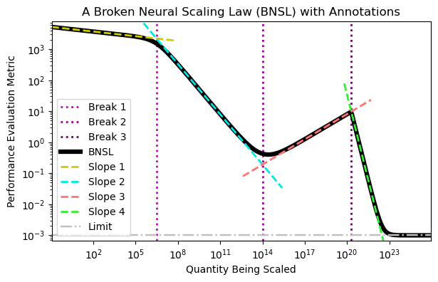
Figure 1: A Broken Neural Scaling Law (BNSL) (dark black solid line) (with 3 breaks where purple dotted lines intersect with dark black solid line) that contains 4 individual power law segments (where the dashed lines that are yellow, blue, red, and green overlap with the dark black solid line). The 1st and 2nd break are very smooth; the 3rd break is very sharp. See Section 2 for more details.

The general functional form of a broken neural scaling law (BNSL) is given as follows:

$$\vspace{-1.0mm}y=a+\bigg{(}bx^{-c_{0}}\bigg{)}\prod_{i=1}^{n}\left(1+\left(\frac{x}{d_{i}}\right)^{1/f_{i}}\right)^{-c_{i}*f_{i}},$$ (1)

where $y$ represents a performance evaluation metric (e.g. prediction error, cross entropy, calibration error, AUROC, BLEU score percentage, F1 score, reward, Elo rating, or FID score) (downstream or upstream) and $x$ represents a quantity that is being scaled (e.g. number of model parameters, amount of compute used for training (or inference), training dataset size, model input size, number of training steps, or upstream performance). The remaining parameters $a,b,c_{0},c_{1}...c_{n},d_{1}...d_{n},f_{1}...f_{n}$ are unknown constants that must be estimated by fitting the above functional form to the $(x,y)$ data points. (In our experiments, SciPy curve-fitting library (Virtanen et al., 2020) was used.)

The constants in Equation 1 above are interpreted as follows. Constant $n$ represents the number of (smooth) “breaks” (i.e. transitions) between $n+1$ consecutive approximately linear (on a log-log plot) segments, for a total of $n+1$ approximately linear segments (on a log-log plot); when $n=0$, equation 1 becomes $y=a+bx^{-c_{0}}$. Constant $a$ represents the limit as to how far the value of $y$ (performance evaluation metric) can be reduced (or maximized) even if $x$ (the quantity being scaled) goes to infinity. Constant $b$ represents the offset of functional form on a log-log plot (analogous to the intercept $b$ in $y=mx+b$ on a linear-linear plot). Constant $c_{0}$ represents the slope of the first approximately linear region on a log-log plot. If there is a “slope $=0$” random guessing region (often there is not) at the beginning of the scaling behavior, $c_{0}=0$ and $b=(random\_guessing\_performance-a)$. Constant $c_{i}$ represents the difference in slope of the $(i)$th approximately linear region and the $(i+1)$th approximately linear region on a log-log plot. Constant $d_{i}$ represents where on the x-axis the break between the $(i)$th and the $(i+1)$th approximately linear region (on a log-log plot) occurs. Constant $f_{i}$ represents the sharpness of the break between the $(i)$th and the $(i+1)$th approximately linear region on a log-log plot; smaller (nonnegative) values of $f_{i}$ yield a sharper break and intervals (before and after the $(i)$th break) that are more linear on a log-log plot; larger values of $f_{i}$ yield a smoother (wider) break and intervals (before and after the $(i)$th break) that are less linear on a log-log plot.

For mathematical analysis and explanation of why Equation 1 is smoothly piece-wise (approximately) linear function on a log-log plot, see Appendix A.1. For mathematical decomposition of Equation 1 into the power law segments it is composed of (e.g. as in Figure 1), see Appendix A.2.

Note that, a smoothly connected approximately piece-wise linear (in log-log plot) function such as BNSL can, with enough segments, fit well any smooth univariate function. However, it remained unclear whether BNSL would also extrapolate the scaling behaviors of deep neural networks well; yet as we demonstrate below, it extrapolates quite accurately. Additionally, we find that the number of breaks needed to accurately model an entire scaling behavior is often quite small.

3 Related Work

To the best of our knowledge, Cortes et al. (1994) was the first paper to model the scaling of multilayer neural network’s performance as a power law (also known as a scaling law) (plus a constant) of the form $y=ax^{b}+c$ in which $x$ refers to training dataset size and $y$ refers to test error; we refer to that functional form as M2. Hestness et al. (2017) showed that the functional form, M2, holds over many orders of magnitude. Rosenfeld et al. (2019) demonstrated that the same functional form, M2, applies when $x$ refers to model size (number of parameters). Kaplan et al. (2020) brought “neural” scaling laws to the mainstream & demonstrated that the same functional form, M2, applies when $x$ refers to the amount of compute used for training. Abnar et al. (2021) proposed to use the same functional form, M2, to relate downstream performance to upstream performance. Zhai et al. (2021) & Bansal et al. (2022) introduced the functional form $y=a(x+d)^{b}+c$, (referred to by us as M3) where $d$ represents the scale at which the performance starts to improve beyond the random guess loss (a constant) & transitions to a power law scaling regime. Alabdulmohsin et al. (2022) proposed functional form $(y-\epsilon_{\infty})/((\epsilon_{0}-y)^{a})=bx^{c}$, (referred to by us as M4) where $\epsilon_{\infty}$ is irreducible entropy of the data distribution and $\epsilon_{0}$ is random guess performance, for relating scale to performance & released a scaling laws benchmark dataset that we use in our experiments.

Hernandez et al. (2021) described a smoothly broken power law functional form (consisting of 5 constants after reducing redundant variables) in equation 6.1 of their paper, when relating scale and downstream performance. While this functional form can be summed with an additional constant representing unimprovable performance to obtain a functional form whose expressivity is equivalent to our BNSL with a single break, it is important to note that (i) Hernandez et al. (2021) describes this form only in the specific context, when exploring how fine-tuning combined with transfer learning scales as a function of the model size - thus, their functional form contains a break only with respect to number of model parameters but not with respect to other input quantities which we do explore such as dataset size, compute, number of training steps, model input size, & upstream performance; (ii) they mentioned this equation in passing and as a result did not try to fit or verify this functional form on any data; (iii) they arrived at it simply via combining the scaling law for transfer (that was the focus of their work) with a scaling law for pretraining data; (iv) they did not identify it as a smoothly broken power law, or note any qualitative advantages of this functional form; (v) they did not discuss the family of functional forms with multiple breaks.

Finally, we would like to mention that smoothly broken power law functional forms, equivalent to equation 1, are commonly used in the astrophysics literature (e.g. dam (2017)) as they happen to model well a variety of physical phenomena. This inspired us to investigate their applicability to a wide range of deep neural scaling phenomena as well.

4 Theoretical Limitations of Previously Proposed Scaling Laws

Our use of BNSLs is inspired by the observation that scaling is not always well predicted by a simple power law; nor are many of the modifications which have been applied in previous works sufficient to capture the qualitative properties of empirical scaling curves. Here we show mathematically two qualitative defects of these functional forms:

1. They are strictly monotonic (first-order derivative does not change its sign) and thus unable to fit double descent phenomena.

2. They cannot express inflection points (second-order derivative does not change its sign), which are frequently observed empirically. An exception to this is M4, proposed by Alabdulmohsin et al. (2022).

Note that some of these functional forms (e.g. M3) can exhibit inflection points on the log-log axes which are commonly used for plotting scaling data (as it was observed in several prior works). However, for inflection points on a linear-linear plot, the extra expressiveness of broken neural scaling laws appears to be necessary (and sufficient). Figure 4 and Figure 5 provide examples of BNSLs producing non-monotonic behavior and inflection points, respectively, establishing the capacity of this functional form to model and extrapolate these phenomena that occur in real scaling behaviors.

name	$f(x)$	$f^{\prime}(x)$	$f^{\prime\prime}(x)$
M1	$ax^{b}$	$abx^{b-1}$	$ab(b-1)x^{b-2}$
M2	$ax^{b}+c$	$abx^{b-1}$	$ab(b-1)x^{b-2}$
M3	$a(x^{-1}+d)^{-b}+c$	$\frac{ab}{x(1+dx)(d+1/x)^{b}}$	$abx^{(b-2)}(1+dx)^{(-2-b)}(b-1-2dx)$

Table 1: Previously proposed functional forms M1, M2, M3 and their (first and second order) derivatives. See Equation 2 for functional form M4.

M1, M2, M3 functional forms cannot model non-monotonic behavior or inflection points: First, recall that expressions of the form $m^{n}$ can only take the value $0$ if $m=0$. We now examine the expressions for the first and second derivatives of M1, M2, M3, provided in Table 1, and observe that they are all continuous and do not have roots over the relevant ranges of their variables, i.e. $x>0$ in general and $b<0$ in the case of M3 (we require $x>0$ because model size, dataset size, and compute are always non-negative). This implies that, for any valid settings of the parameters $a,b,c,d,x$, these functional forms are monotonic (as the first derivative never changes sign), and that they lack inflection points (since an inflection point must have $f^{\prime\prime}(x)=0$).

M4 functional form cannot model non-monotonic behavior. The case of M4 is a bit different, since the relationship between $y$ and $x$ in this case is expressed as an inverse function, i.e.

$$x=g(y)=\left(\frac{y-\epsilon_{\infty}}{b(\epsilon_{0}-y)^{a}}\right)^{1/c}$$ (2)

However, non-monotonicity of $y$ as an inverse function $y=g^{-1}(x)$ is ruled out, since that would imply two different values of $x=g(y)$ can be obtained for the single value of $y$ – this is impossible, since $f(y)$ maps each $y$ deterministically to a single value of $x$. As a result, M4 cannot express non-monotonic functions.

M4 functional form can model inflection points. It is easy to see that if $y=g^{-1}(x)$ had an inflection point, then $x=g(y)$ would have it as well. This is because an inflection point is defined as a point $x$ where $f(x)$ changes from concave to convex, which implies that $g(y)$ changes from convex to concave, since the inverse of a convex function is concave; the root(s) of $g^{\prime\prime}(y)$ are the point(s) at which this change occurs. Using Wolfram Alpha and matplotlib (Hunter, 2007), we observe that M4 is able to express inflection points, e.g. $(a,b,c,\epsilon_{0},\epsilon_{\infty},x,y)=(1,1,-2,3/4,1/4,1/\sqrt{3},5/8$), or $(a,b,c,\epsilon_{0},\epsilon_{\infty},x,y)=(2,1,-3,2/3,1/3,(-5/6+\sqrt{3}/2)^{1/3},1/\sqrt{3})$.

5 Empirical Results: Fits & Extrapolations of Functional Forms

We now show the fits & extrapolations of various functional forms. In all plots here, onward, & in the appendix, black points are points used for fitting a functional form, green (gray if color blind) points are held-out points used for evaluating extrapolation of functional form fit to the black points, & a red line is BNSL that has been fit to black points. 100% of the plots in this paper here, onward, & in the appendix contain green point(s) for evaluating extrapolation. See Section A.6 for details on fitting BNSL & determining the number of breaks. Except when stated otherwise, each plot contains the region(s) surrounding (or neighboring) a single break of a BNSL fit to black points that are smaller (along the x-axis) than the green points.

All the extrapolation evaluations reported in the tables (that have $\downarrow$ symbol in the top row) are reported in terms of root mean squared log error (RMSLE) ± root standard log error. See Appendix A.3 for definition of RMSLE and Appendix A.4 for definition of root standard log error.

Domain		M1 $\uparrow$	M2 $\uparrow$	M3 $\uparrow$	M4 $\uparrow$	BNSL $\uparrow$
Downstream Image Classification		2.78%	4.17%	9.72%	13.89%	69.44%
Language (Downstream and Upstream)		10%	5%	10%	0%	75%

Table 2: Percentage of tasks by domain where each functional form is the best for extrapolation of scaling behavior. Numbers for M1, M2, M3, and M4 were obtained via correspondence with authors of Alabdulmohsin et al. (2022). See Sections 5.1 and 5.2 for more details.

5.1 Vision

Using the scaling laws benchmark of Alabdulmohsin et al. (2022), we evaluate how well various functional forms extrapolate performance on downstream vision tasks as upstream training dataset size increases. In this large-scale vision subset of the benchmark, the tasks that are evaluated are error rate on each of various few-shot downstream image classification (IC) tasks; the downstream tasks are: Birds 200 (Welinder et al., 2010), Caltech101 (Fei-Fei et al., 2004), CIFAR-100 (Krizhevsky et al., 2009), and ImageNet (Deng et al., 2009). The following architectures of various sizes are pretrained on subsets of JFT-300M (Sun et al., 2017): big-transfer residual neural networks (BiT) (Kolesnikov et al., 2020), MLP mixers (MiX) (Tolstikhin et al., 2021), and vision transformers (ViT) (Dosovitskiy et al., 2020). As can be seen in Tables 2 and 3, BNSL yields extrapolations with the lowest RMSLE (Root Mean Squared Logarithmic Error) for 69.44% of tasks of any of the functional forms, while the next best functional form performs the best on only 13.89% of the tasks.

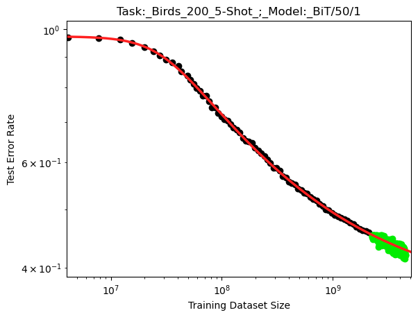
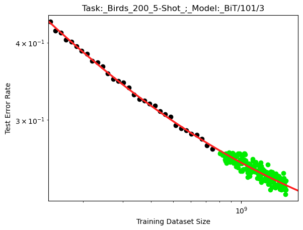
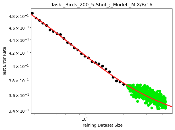
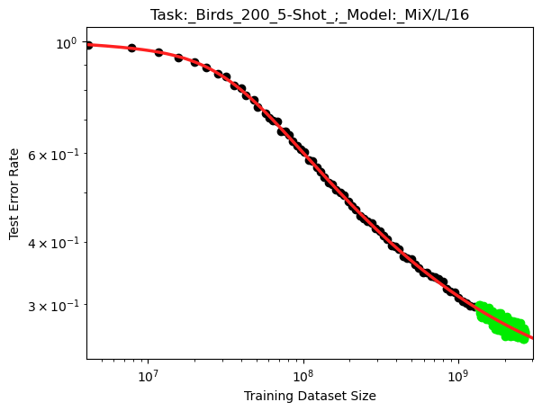
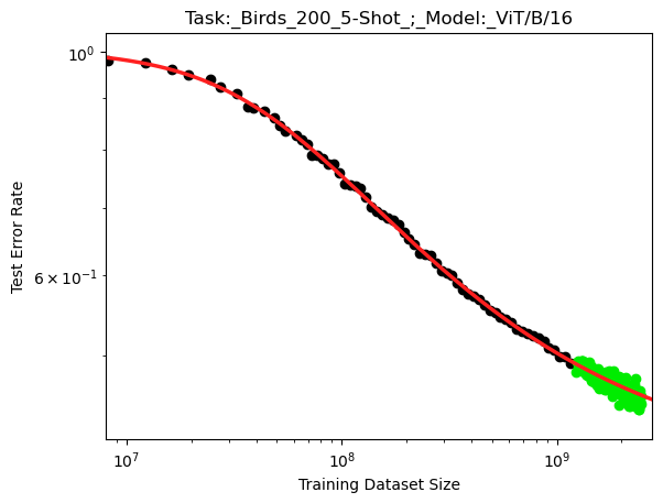
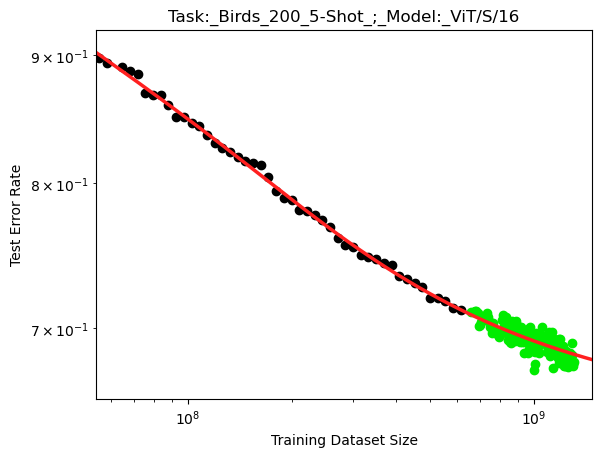
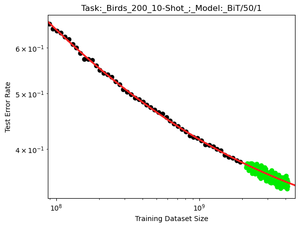
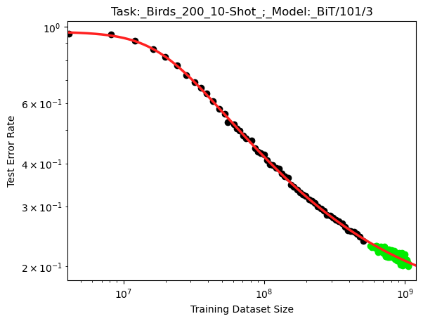
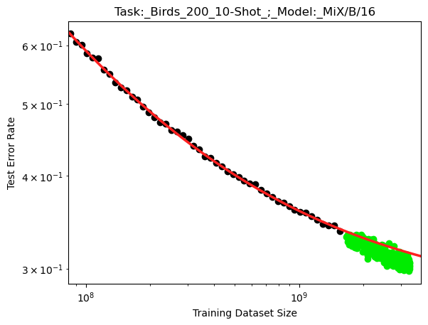
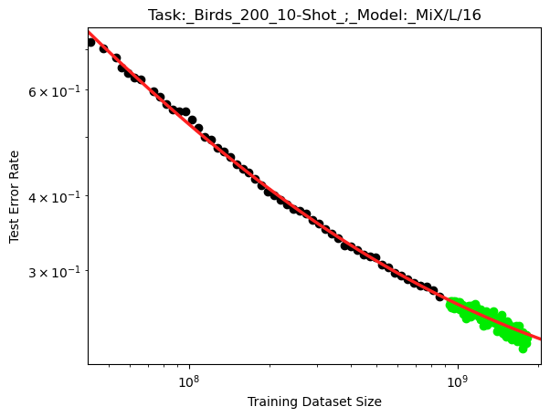
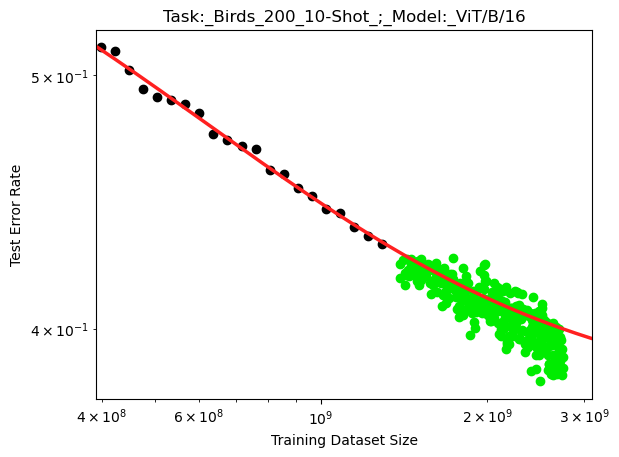
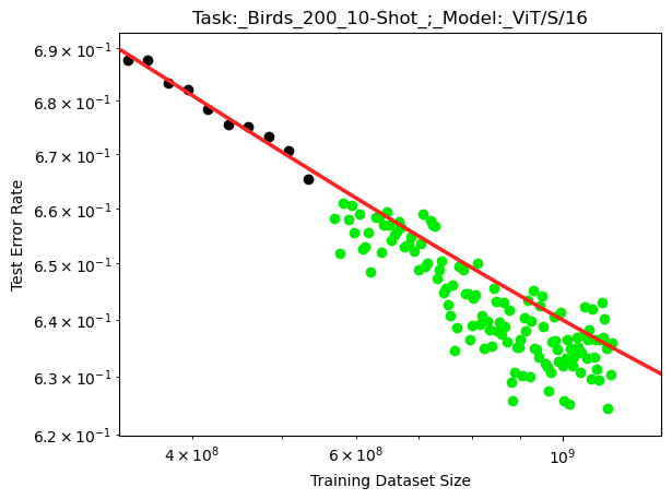
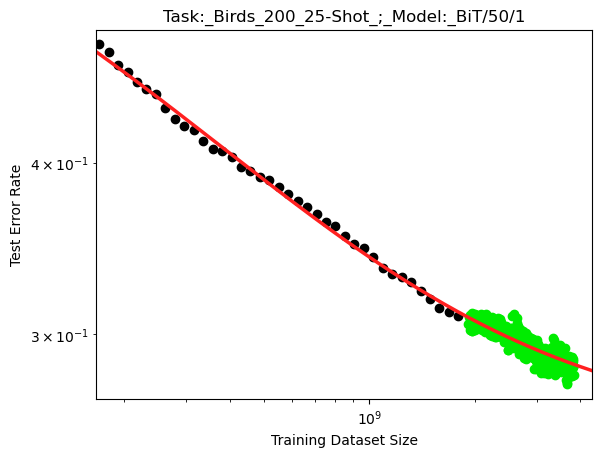
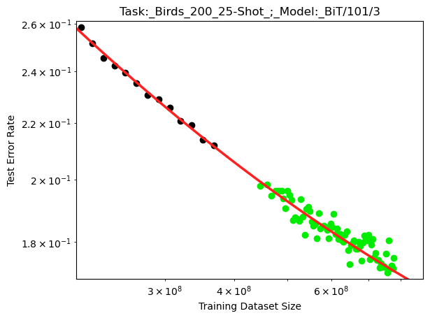
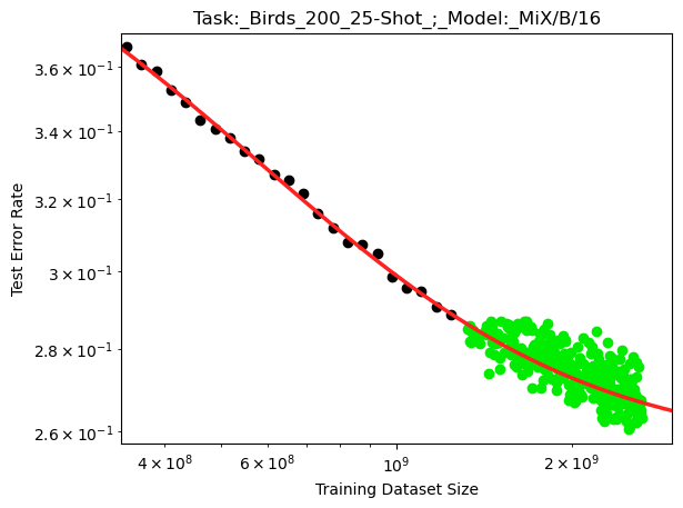
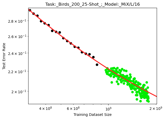
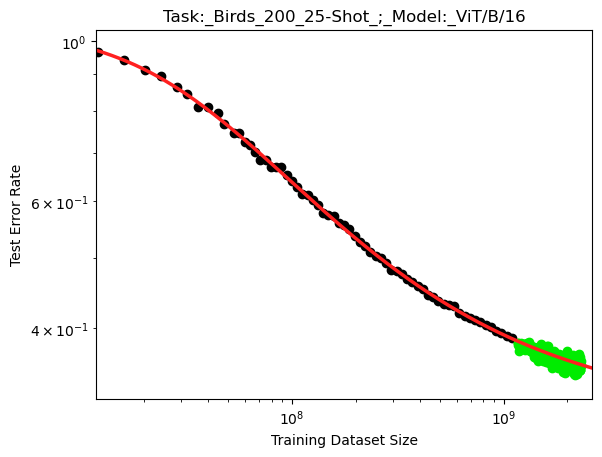
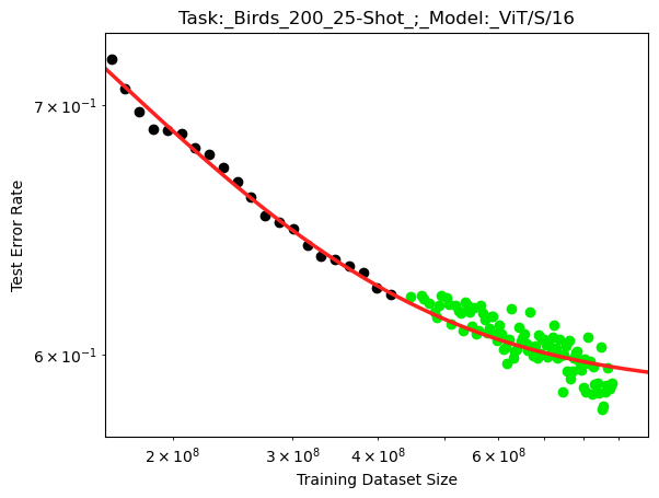
Figure 34: Extrapolation Results of BNSL on Downstream Birds 200. X-axis is pretraining dataset size. See Section 5.1 for more details.

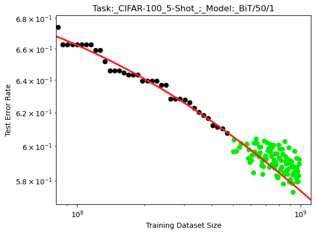
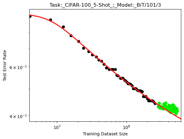
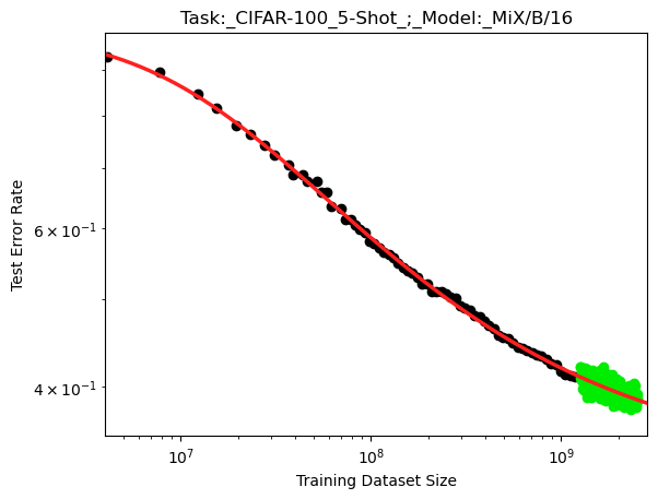
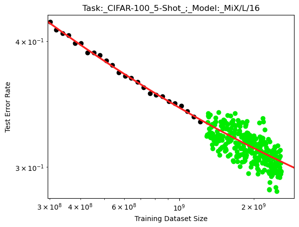
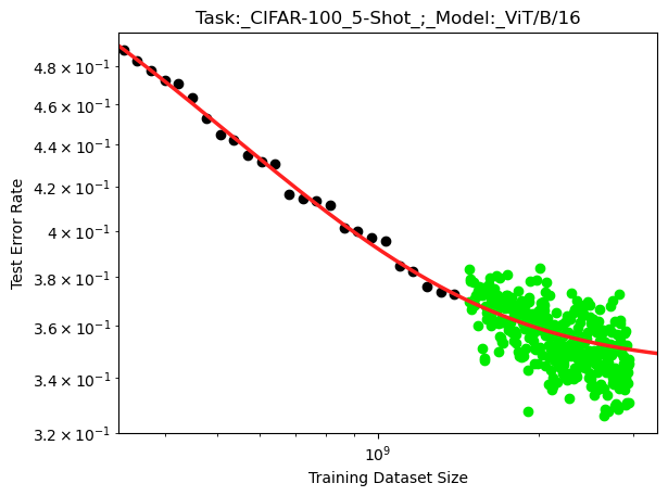
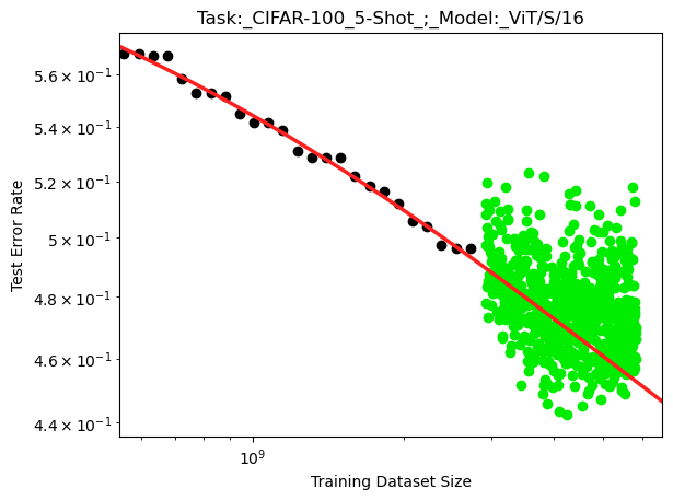
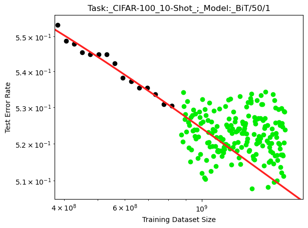
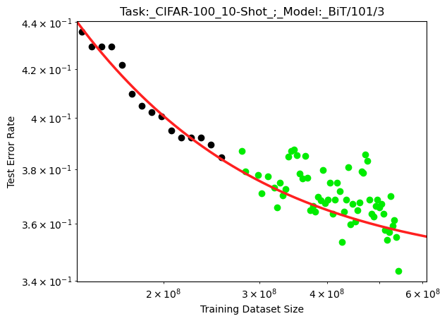
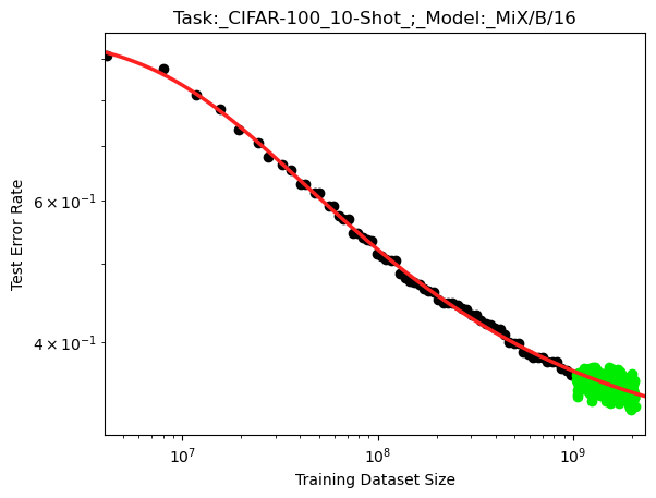
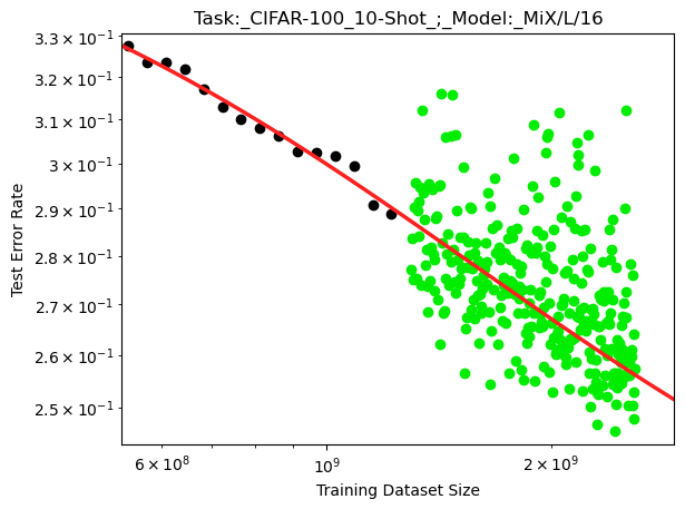
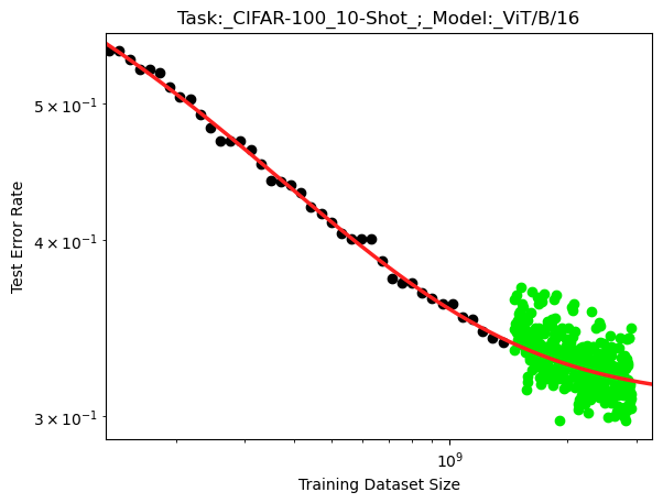
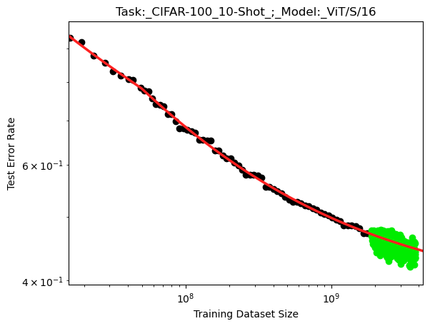
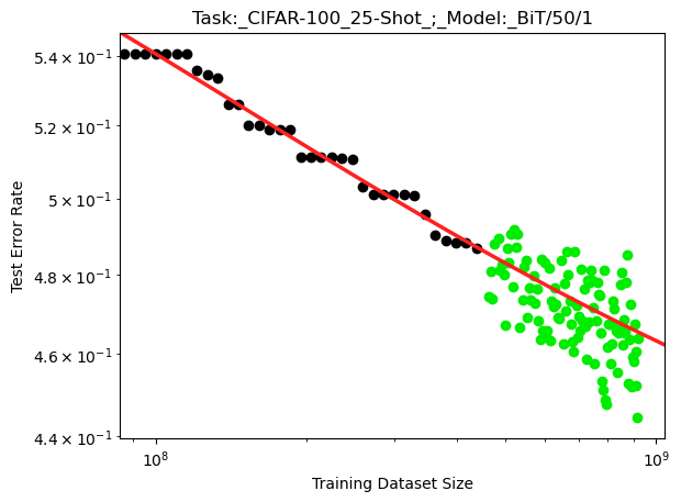
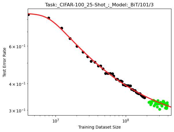
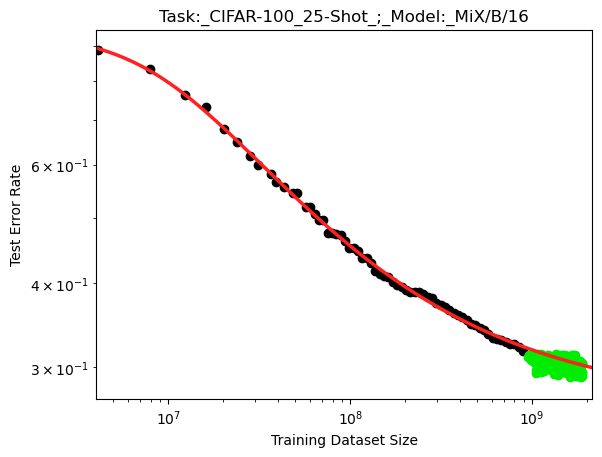
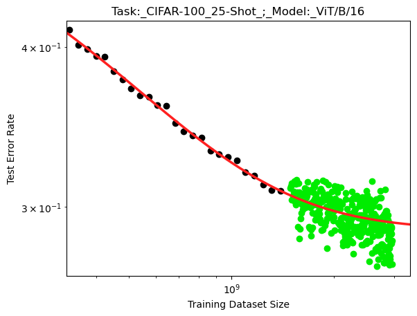
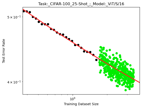
Figure 35: Extrapolation Results of BNSL on Downstream CIFAR-100. X-axis is pretraining dataset size. See Section 5.1 for more details.

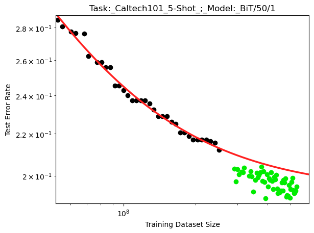
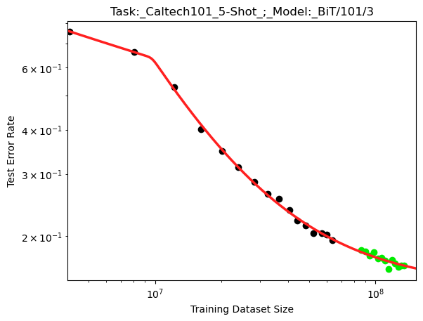
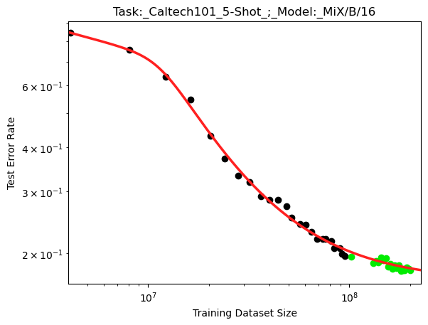
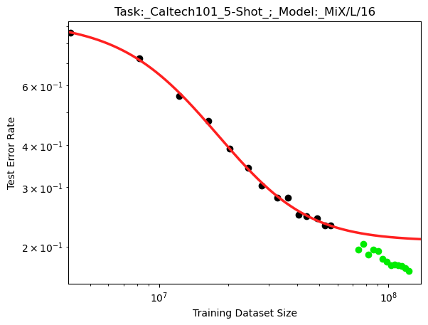
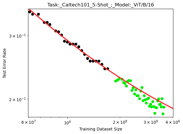
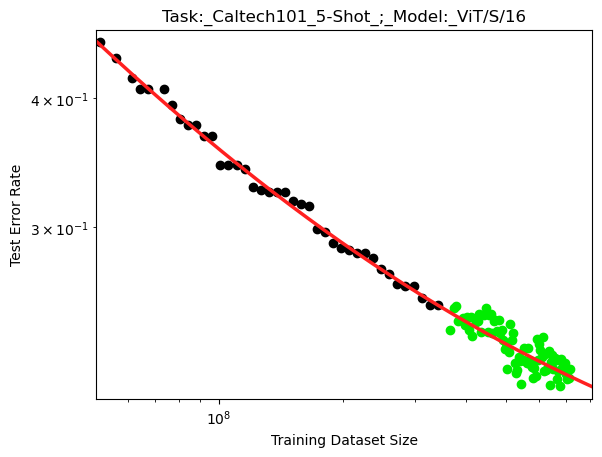
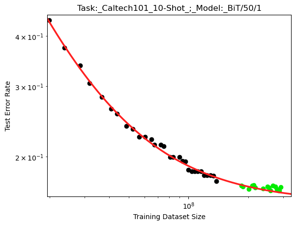
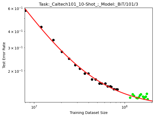
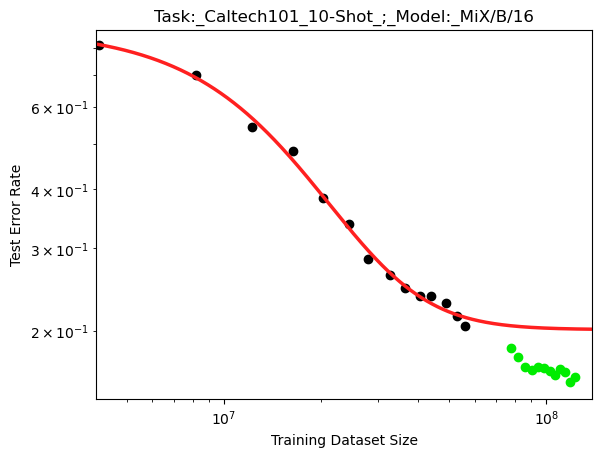
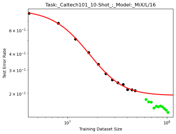
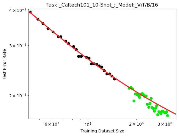
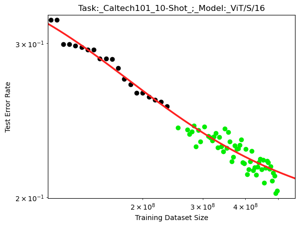
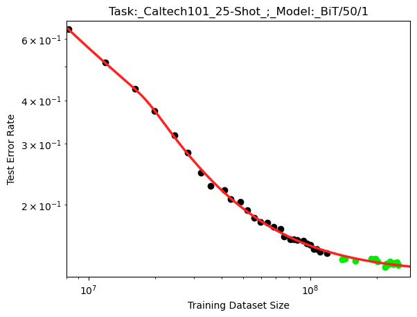
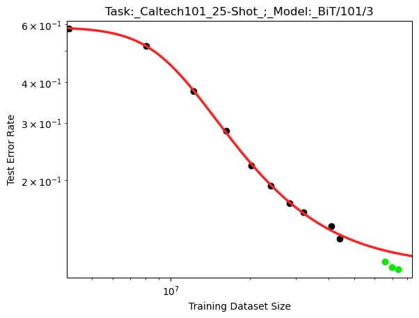
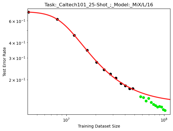
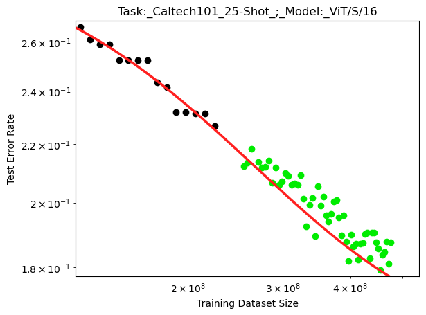
Figure 36: Extrapolation Results of BNSL on Downstream Caltech101. X-axis is pretraining dataset size. See Section 5.1 for more details. From eyeballing, we think the subset of Caltech101 with unsatisfactory extrapolations has unsatisfactory extrapolations due to the maximum (along the x-axis) of the black point used for fitting being near or before a break; this is accentuated by not having enough points for fitting for the SciPy fitter to be able to determine whether the break is an actual break or just noisy deviation. See Section 6 for more details on this explanation.

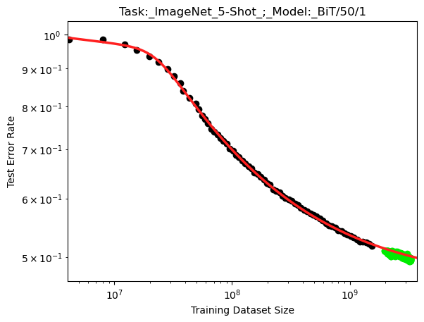
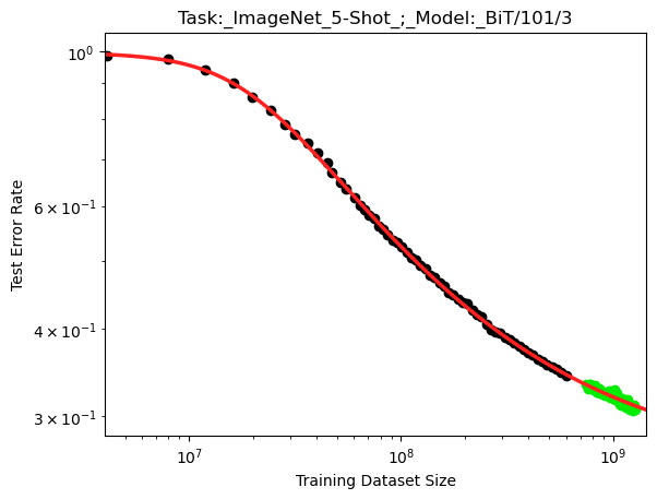
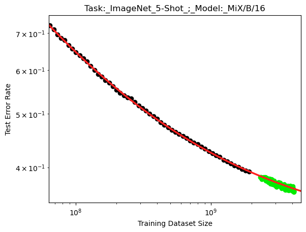
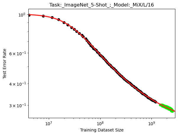
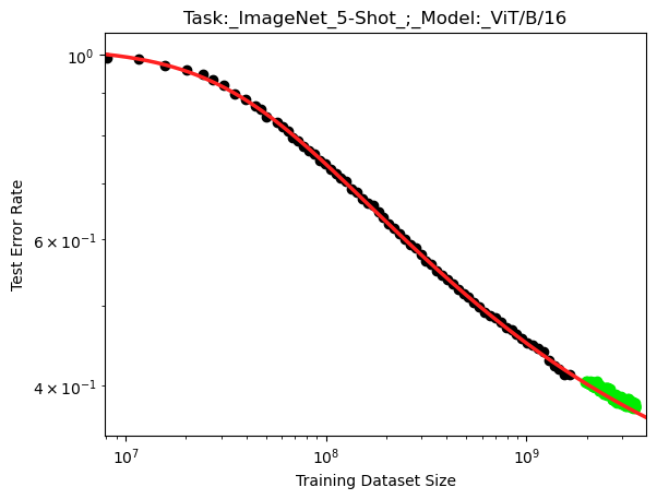
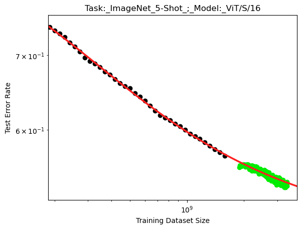
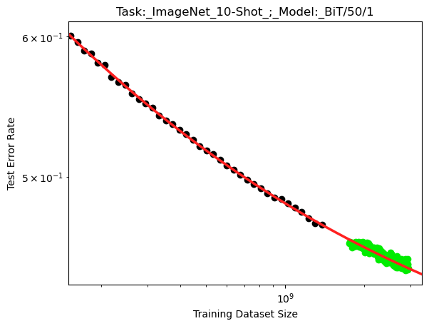
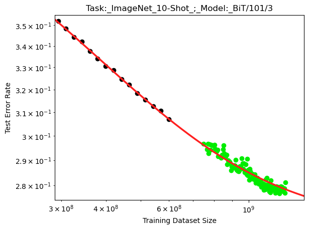
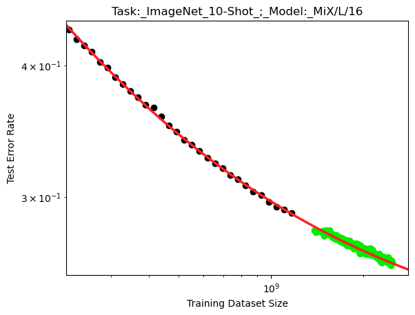
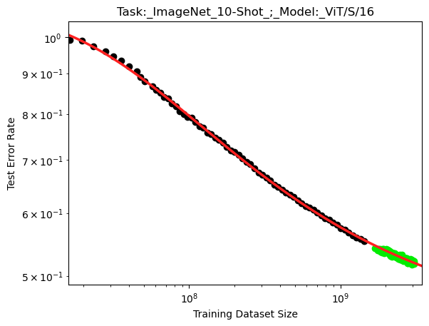
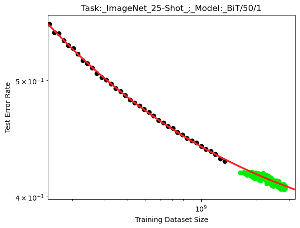
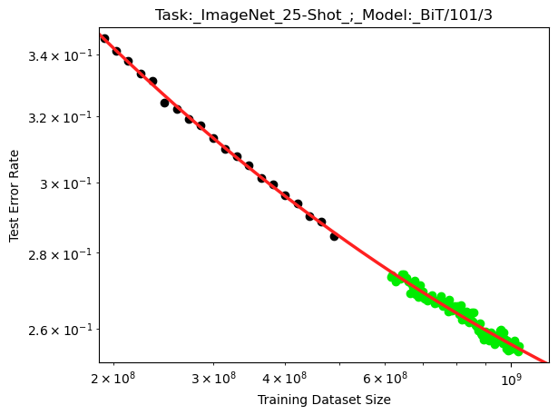
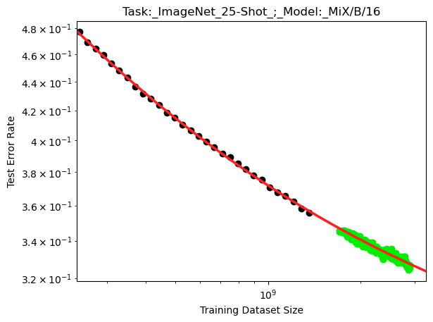
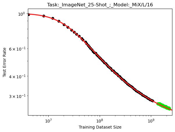
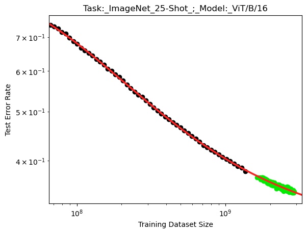
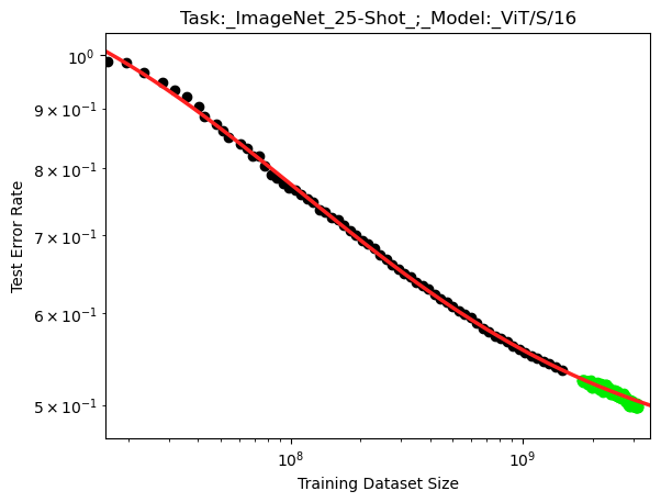
Figure 40: Extrapolation Results of BNSL on Downstream ImageNet. X-axis is pretraining dataset size. See Section 5.1 for more details.

To view plots of BNSL on each of these tasks, see figures 34, 35, 36, 40 in Appendix A.36. To view plots of M1, M2, M3, M4 on each of these tasks, see Appendix A.4 of Alabdulmohsin et al. (2022).

In Section A.9, we additionally show that BNSL yields accurate extrapolations of performance on large-scale downstream vision tasks when amount of compute used for (pre-)training is on the x-axis and compute is scaled in the manner that is Pareto optimal with respect to the performance evaluation metric on the y-axis (downstream accuracy in this case).

In Section A.11, we additionally show that BNSL yields accurate extrapolations of the scaling behavior of diffusion generative models of images.

In Section A.12, we additionally show that BNSL yields accurate extrapolations of the scaling behavior of generative models of video.

In Section A.24, we show that BNSL yields accurate extrapolations of robotics scaling behavior (out-of-distribution (OOD) generalization and in-distribution generalization).

In Section A.23, BNSL accurately extrapolates the scaling behavior of continual learning.

In Section A.19, BNSL accurately extrapolates the scaling behavior of adversarial robustness.

In Section A.30, BNSL accurately extrapolates the scaling behavior of fairness (and also ensembles).

In Section A.33, we show that BNSL accurately extrapolates the scaling behavior of the downstream performance of multimodal contrastive learning (e.g. non-generative unsupervised learning).

In Section A.13, we additionally show that BNSL yields accurate extrapolations of the scaling behavior when data is pruned Pareto optimally (such that each point along the x-axis uses the subset of the dataset that yields the best performance (y-axis value) for that dataset size (x-axis value)).

In Section A.14, we additionally show that BNSL yields accurate extrapolations when upstream performance is on the x-axis and downstream performance is on the y-axis.

In Section A.8 (and Figure 2), we additionally show that BNSL accurately extrapolates downstream performance to scales that are over an order of magnitude larger than the maximum (along the x-axis) of the points used for fitting.

Task	Model		M1 $\downarrow$	M2 $\downarrow$	M3 $\downarrow$	M4 $\downarrow$	BNSL $\downarrow$
Birds 200 10-shot	BiT/101/3		9.13e-2 ± 2.8e-3	9.13e-2 ± 2.8e-3	9.13e-2 ± 2.8e-3	2.95e-2 ± 1.3e-3	1.76e-2 ± 1.1e-3
Birds 200 10-shot	BiT/50/1		6.88e-2 ± 7.5e-4	6.88e-2 ± 7.5e-4	5.24e-2 ± 6.2e-4	2.66e-2 ± 5.3e-4	1.19e-2 ± 3.5e-4
Birds 200 10-shot	MiX/B/16		9.15e-2 ± 1.1e-3	9.15e-2 ± 1.1e-3	3.95e-2 ± 7.0e-4	4.62e-2 ± 8.2e-4	3.04e-2 ± 6.9e-4
Birds 200 10-shot	MiX/L/16		5.51e-2 ± 1.4e-3	5.51e-2 ± 1.4e-3	5.51e-2 ± 1.4e-3	5.15e-2 ± 1.7e-3	1.85e-2 ± 8.9e-4
Birds 200 10-shot	ViT/B/16		6.77e-2 ± 1.1e-3	6.77e-2 ± 1.1e-3	3.52e-2 ± 8.1e-4	1.51e-2 ± 6.2e-4	1.69e-2 ± 7.0e-4
Birds 200 10-shot	ViT/S/16		3.95e-2 ± 1.2e-3	3.95e-2 ± 1.2e-3	3.74e-2 ± 1.1e-3	1.85e-2 ± 7.9e-4	1.09e-2 ± 6.1e-4
Birds 200 25-shot	BiT/101/3		9.41e-2 ± 3.2e-3	9.41e-2 ± 3.2e-3	9.41e-2 ± 3.2e-3	6.38e-2 ± 2.0e-3	1.55e-2 ± 1.3e-3
Birds 200 25-shot	BiT/50/1		1.10e-1 ± 1.0e-3	7.29e-2 ± 8.0e-4	1.52e-2 ± 4.9e-4	1.97e-2 ± 5.6e-4	1.33e-2 ± 4.4e-4
Birds 200 25-shot	MiX/B/16		1.40e-1 ± 1.9e-3	1.40e-1 ± 1.9e-3	6.93e-2 ± 1.2e-3	2.11e-2 ± 6.9e-4	1.64e-2 ± 6.6e-4
Birds 200 25-shot	MiX/L/16		1.12e-1 ± 2.0e-3	1.12e-1 ± 2.0e-3	1.12e-1 ± 2.0e-3	5.44e-2 ± 1.8e-3	2.08e-2 ± 1.1e-3
Birds 200 25-shot	ViT/B/16		9.02e-2 ± 1.6e-3	9.02e-2 ± 1.6e-3	3.75e-2 ± 1.0e-3	1.51e-2 ± 5.7e-4	1.62e-2 ± 6.1e-4
Birds 200 25-shot	ViT/S/16		5.06e-2 ± 1.4e-3	5.06e-2 ± 1.4e-3	4.96e-2 ± 1.4e-3	4.02e-2 ± 1.2e-3	1.03e-2 ± 6.6e-4
Birds 200 5-shot	BiT/101/3		8.17e-2 ± 2.0e-3	8.17e-2 ± 2.0e-3	8.17e-2 ± 2.0e-3	3.38e-2 ± 1.3e-3	1.81e-2 ± 8.2e-4
Birds 200 5-shot	BiT/50/1		5.44e-2 ± 5.6e-4	5.44e-2 ± 5.6e-4	5.44e-2 ± 5.6e-4	2.59e-2 ± 5.4e-4	1.34e-2 ± 3.7e-4
Birds 200 5-shot	MiX/B/16		8.27e-2 ± 1.0e-3	8.27e-2 ± 1.0e-3	5.49e-2 ± 7.8e-4	2.14e-2 ± 5.3e-4	1.39e-2 ± 4.1e-4
Birds 200 5-shot	MiX/L/16		5.68e-2 ± 1.4e-3	5.68e-2 ± 1.4e-3	5.68e-2 ± 1.4e-3	3.20e-2 ± 9.7e-4	1.85e-2 ± 6.4e-4
Birds 200 5-shot	ViT/B/16		3.40e-2 ± 8.9e-4	3.40e-2 ± 8.9e-4	3.40e-2 ± 8.9e-4	1.65e-2 ± 6.7e-4	1.36e-2 ± 5.8e-4
Birds 200 5-shot	ViT/S/16		2.75e-2 ± 7.9e-4	2.75e-2 ± 7.9e-4	2.75e-2 ± 7.9e-4	1.20e-2 ± 5.2e-4	7.39e-3 ± 4.5e-4
CIFAR-100 10-shot	BiT/101/3		8.57e-2 ± 3.8e-3	8.57e-2 ± 3.8e-3	8.25e-2 ± 3.7e-3	4.77e-2 ± 3.0e-3	2.58e-2 ± 2.3e-3
CIFAR-100 10-shot	BiT/50/1		7.44e-2 ± 1.5e-3	1.24e-2 ± 5.8e-4	2.08e-2 ± 7.2e-4	1.24e-2 ± 5.8e-4	1.83e-2 ± 8.3e-4
CIFAR-100 10-shot	MiX/B/16		8.77e-2 ± 1.9e-3	8.77e-2 ± 1.9e-3	2.71e-2 ± 1.2e-3	2.37e-2 ± 9.9e-4	2.44e-2 ± 9.5e-4
CIFAR-100 10-shot	MiX/L/16		1.05e-1 ± 3.1e-3	1.05e-1 ± 3.1e-3	4.85e-2 ± 2.6e-3	4.97e-2 ± 1.6e-3	4.75e-2 ± 2.6e-3
CIFAR-100 10-shot	ViT/B/16		8.98e-2 ± 2.0e-3	8.98e-2 ± 2.0e-3	8.98e-2 ± 2.0e-3	4.98e-2 ± 1.7e-3	3.71e-2 ± 1.4e-3
CIFAR-100 10-shot	ViT/S/16		6.84e-2 ± 1.1e-3	2.11e-2 ± 6.6e-4	3.35e-2 ± 8.6e-4	2.54e-2 ± 7.5e-4	2.57e-2 ± 7.5e-4
CIFAR-100 25-shot	BiT/101/3		8.77e-2 ± 5.6e-3	8.77e-2 ± 5.6e-3	4.44e-2 ± 3.5e-3	3.40e-2 ± 2.7e-3	2.88e-2 ± 3.0e-3
CIFAR-100 25-shot	BiT/50/1		7.31e-2 ± 2.0e-3	2.35e-2 ± 1.5e-3	3.65e-2 ± 1.8e-3	2.35e-2 ± 1.5e-3	1.89e-2 ± 1.1e-3
CIFAR-100 25-shot	MiX/B/16		1.08e-1 ± 2.3e-3	4.75e-2 ± 1.6e-3	2.10e-2 ± 9.4e-4	2.24e-2 ± 9.9e-4	2.67e-2 ± 1.1e-3
CIFAR-100 25-shot	MiX/L/16		9.79e-2 ± 2.2e-3	9.79e-2 ± 2.2e-3	3.67e-2 ± 1.7e-3	2.98e-2 ± 1.4e-3	3.45e-2 ± 1.6e-3
CIFAR-100 25-shot	ViT/B/16		1.07e-1 ± 1.9e-3	1.07e-1 ± 1.9e-3	6.54e-2 ± 1.6e-3	4.80e-2 ± 1.4e-3	3.02e-2 ± 4.5e-3
CIFAR-100 25-shot	ViT/S/16		8.03e-2 ± 1.2e-3	2.19e-2 ± 7.4e-4	3.13e-2 ± 8.4e-4	2.27e-2 ± 7.1e-4	2.14e-2 ± 6.9e-4
CIFAR-100 5-shot	BiT/101/3		5.94e-2 ± 3.2e-3	5.94e-2 ± 3.2e-3	5.94e-2 ± 3.2e-3	3.30e-2 ± 2.4e-3	3.78e-2 ± 2.6e-3
CIFAR-100 5-shot	BiT/50/1		4.87e-2 ± 1.3e-3	4.87e-2 ± 1.3e-3	1.69e-2 ± 8.8e-4	1.87e-2 ± 8.9e-4	1.45e-2 ± 8.7e-4
CIFAR-100 5-shot	MiX/B/16		7.07e-2 ± 1.2e-3	7.07e-2 ± 1.2e-3	2.78e-2 ± 8.4e-4	1.76e-2 ± 6.6e-4	1.70e-2 ± 6.3e-4
CIFAR-100 5-shot	MiX/L/16		7.06e-2 ± 1.6e-3	7.06e-2 ± 1.6e-3	4.17e-2 ± 1.4e-3	3.32e-2 ± 1.2e-3	2.77e-2 ± 1.0e-3
CIFAR-100 5-shot	ViT/B/16		6.27e-2 ± 1.6e-3	6.27e-2 ± 1.6e-3	6.27e-2 ± 1.6e-3	4.30e-2 ± 1.3e-3	2.82e-2 ± 1.0e-3
CIFAR-100 5-shot	ViT/S/16		6.93e-2 ± 1.2e-3	2.84e-2 ± 8.2e-4	3.88e-2 ± 8.0e-4	3.16e-2 ± 7.5e-4	3.50e-2 ± 9.2e-3
Caltech101 10-shot	BiT/101/3		3.07e-1 ± 2.0e-2	3.07e-1 ± 2.0e-2	1.51e-1 ± 1.3e-2	1.00e-1 ± 1.1e-2	4.75e-2 ± 8.1e-3
Caltech101 10-shot	BiT/50/1		3.29e-1 ± 1.6e-2	7.68e-2 ± 5.0e-3	1.13e-1 ± 6.0e-3	6.01e-2 ± 4.4e-3	1.77e-2 ± 2.5e-3
Caltech101 10-shot	MiX/B/16		1.35e-1 ± 1.4e-2	1.35e-1 ± 1.4e-2	1.35e-1 ± 1.4e-2	1.92e-1 ± 1.6e-2	2.04e-1 ± 9.7e-3
Caltech101 10-shot	MiX/L/16		1.25e-1 ± 1.3e-2	1.25e-1 ± 1.3e-2	1.25e-1 ± 1.3e-2	1.30e-1 ± 1.2e-2	2.13e-1 ± 1.5e-2
Caltech101 10-shot	ViT/B/16		7.76e-2 ± 4.3e-3	7.76e-2 ± 4.3e-3	3.11e-2 ± 3.0e-3	5.75e-2 ± 4.4e-3	4.02e-2 ± 3.9e-3
Caltech101 10-shot	ViT/S/16		1.95e-1 ± 6.0e-3	3.41e-2 ± 2.9e-3	2.40e-2 ± 2.0e-3	3.41e-2 ± 2.9e-3	2.40e-2 ± 2.0e-3
Caltech101 25-shot	BiT/101/3		1.15e-1 ± 6.5e-3	1.15e-1 ± 6.5e-3	1.15e-1 ± 6.5e-3	1.15e-1 ± 6.5e-3	9.86e-2 ± 8.0e-3
Caltech101 25-shot	BiT/50/1		3.60e-1 ± 1.9e-2	8.80e-2 ± 5.5e-3	1.43e-1 ± 7.6e-3	4.76e-2 ± 3.6e-3	1.55e-2 ± 1.6e-3
Caltech101 25-shot	MiX/B/16		8.28e-2 ± 1.2e-2	8.28e-2 ± 1.2e-2	8.28e-2 ± 1.2e-2	1.65e-1 ± 1.7e-2	1.93e-1 ± 1.3e-2
Caltech101 25-shot	MiX/L/16		9.66e-2 ± 1.0e-2	9.66e-2 ± 1.0e-2	9.66e-2 ± 1.0e-2	9.66e-2 ± 1.0e-2	1.49e-1 ± 1.3e-2
Caltech101 25-shot	ViT/B/16		1.03e-1 ± 5.6e-3	3.33e-2 ± 2.5e-3	4.46e-2 ± 3.6e-3	3.33e-2 ± 2.5e-3	3.95e-2 ± 5.4e-3
Caltech101 25-shot	ViT/S/16		1.77e-1 ± 5.4e-3	3.79e-2 ± 3.1e-3	2.80e-2 ± 1.8e-3	3.79e-2 ± 3.1e-3	3.29e-2 ± 2.1e-3
Caltech101 5-shot	BiT/101/3		2.12e-1 ± 1.2e-2	2.12e-1 ± 1.2e-2	2.12e-1 ± 1.2e-2	1.65e-1 ± 9.4e-3	1.87e-2 ± 4.3e-3
Caltech101 5-shot	BiT/50/1		2.34e-1 ± 6.1e-3	4.13e-2 ± 2.1e-3	1.61e-2 ± 1.3e-3	4.69e-2 ± 2.1e-3	4.10e-2 ± 2.1e-3
Caltech101 5-shot	MiX/B/16		2.43e-1 ± 1.2e-2	2.43e-1 ± 1.2e-2	2.35e-1 ± 1.1e-2	7.28e-2 ± 4.3e-3	1.92e-2 ± 1.9e-3
Caltech101 5-shot	MiX/L/16		1.38e-1 ± 9.7e-3	1.38e-1 ± 9.7e-3	1.38e-1 ± 9.7e-3	1.37e-1 ± 9.9e-3	1.63e-1 ± 1.1e-2
Caltech101 5-shot	ViT/B/16		1.10e-1 ± 6.3e-3	1.10e-1 ± 6.3e-3	6.02e-2 ± 4.7e-3	6.81e-2 ± 4.8e-3	3.87e-2 ± 3.4e-3
Caltech101 5-shot	ViT/S/16		1.90e-1 ± 4.7e-3	3.82e-2 ± 2.6e-3	5.04e-2 ± 2.9e-3	3.82e-2 ± 2.6e-3	2.78e-2 ± 1.8e-3
ImageNet 10-shot	BiT/101/3		1.27e-1 ± 2.0e-3	1.27e-1 ± 2.0e-3	7.36e-2 ± 1.1e-3	3.06e-2 ± 7.0e-4	6.65e-3 ± 3.8e-4
ImageNet 10-shot	BiT/50/1		9.54e-2 ± 7.2e-4	9.54e-2 ± 7.2e-4	5.75e-3 ± 2.0e-4	1.86e-2 ± 2.8e-4	3.84e-3 ± 1.5e-4
ImageNet 10-shot	MiX/B/16		9.34e-2 ± 7.9e-4	9.34e-2 ± 7.9e-4	3.37e-2 ± 2.9e-4	2.32e-2 ± 3.0e-4	4.22e-3 ± 1.5e-4
ImageNet 10-shot	MiX/L/16		9.83e-2 ± 1.3e-3	9.83e-2 ± 1.3e-3	9.83e-2 ± 1.3e-3	4.01e-3 ± 1.9e-4	4.33e-3 ± 1.8e-4
ImageNet 10-shot	ViT/B/16		4.62e-2 ± 7.1e-4	4.62e-2 ± 7.1e-4	4.62e-2 ± 7.1e-4	1.44e-2 ± 3.0e-4	5.70e-3 ± 2.0e-4
ImageNet 10-shot	ViT/S/16		4.74e-2 ± 5.6e-4	4.74e-2 ± 5.6e-4	1.66e-2 ± 2.5e-4	7.18e-3 ± 2.0e-4	3.71e-3 ± 1.4e-4
ImageNet 25-shot	BiT/101/3		1.42e-1 ± 2.3e-3	1.42e-1 ± 2.3e-3	6.67e-2 ± 9.1e-4	3.31e-2 ± 8.7e-4	4.76e-3 ± 2.8e-4
ImageNet 25-shot	BiT/50/1		1.17e-1 ± 9.2e-4	1.17e-1 ± 9.2e-4	4.06e-3 ± 1.7e-4	1.84e-2 ± 2.6e-4	4.67e-3 ± 1.6e-4
ImageNet 25-shot	MiX/B/16		9.59e-2 ± 9.3e-4	9.59e-2 ± 9.3e-4	5.39e-2 ± 4.9e-4	2.04e-2 ± 3.1e-4	4.17e-3 ± 1.7e-4
ImageNet 25-shot	MiX/L/16		1.03e-1 ± 1.3e-3	1.03e-1 ± 1.3e-3	1.03e-1 ± 1.3e-3	6.33e-3 ± 2.2e-4	7.60e-3 ± 2.6e-4
ImageNet 25-shot	ViT/B/16		5.17e-2 ± 8.8e-4	5.17e-2 ± 8.8e-4	5.17e-2 ± 8.8e-4	1.52e-2 ± 3.8e-4	4.96e-3 ± 2.0e-4
ImageNet 25-shot	ViT/S/16		5.52e-2 ± 4.4e-4	4.12e-2 ± 3.4e-4	9.65e-3 ± 2.3e-4	7.78e-3 ± 2.1e-4	6.11e-3 ± 2.4e-4
ImageNet 5-shot	BiT/101/3		9.24e-2 ± 1.4e-3	9.24e-2 ± 1.4e-3	9.24e-2 ± 1.4e-3	2.09e-2 ± 7.9e-4	8.05e-3 ± 5.0e-4
ImageNet 5-shot	BiT/50/1		8.95e-2 ± 6.7e-4	8.95e-2 ± 6.7e-4	1.53e-2 ± 2.2e-4	1.11e-2 ± 2.3e-4	7.94e-3 ± 2.1e-4
ImageNet 5-shot	MiX/B/16		9.09e-2 ± 7.2e-4	9.09e-2 ± 7.2e-4	3.01e-2 ± 2.8e-4	1.95e-2 ± 2.7e-4	6.49e-3 ± 2.2e-4
ImageNet 5-shot	MiX/L/16		7.99e-2 ± 9.7e-4	7.99e-2 ± 9.7e-4	7.99e-2 ± 9.7e-4	9.92e-3 ± 4.5e-4	5.68e-3 ± 2.4e-4
ImageNet 5-shot	ViT/B/16		4.11e-2 ± 6.3e-4	4.11e-2 ± 6.3e-4	4.11e-2 ± 6.3e-4	1.55e-2 ± 2.8e-4	1.29e-2 ± 2.7e-4
ImageNet 5-shot	ViT/S/16		4.20e-2 ± 4.1e-4	4.20e-2 ± 4.1e-4	2.40e-2 ± 2.6e-4	8.02e-3 ± 1.9e-4	4.72e-3 ± 1.6e-4

Table 3: Extrapolation Results on scaling behavior of Downstream Vision Tasks (also known as Transfer Learning). See Section 5.1 for more details. Numbers for M1, M2, M3, and M4 obtained via correspondence with authors of Alabdulmohsin et al. (2022).

5.2 Language

Using the scaling laws benchmark of Alabdulmohsin et al. (2022), we evaluate how well various functional forms extrapolate performance on language tasks as the (pre-)training dataset size increases. In this large-scale language subset of the benchmark, the tasks that are evaluated are error rates on each of the various downstream tasks from the BIG-Bench (BB) (Srivastava et al., 2022) benchmark and upstream test cross-entropy of various models (e.g. Transformers & occasionally LSTMs) trained to do language modeling (LM) & neural machine translation (NMT). All LM & BB tasks use a decoder-only language model. As can be seen in Tables 2 & 4, BNSL yields extrapolations with the lowest RMSLE (Root Mean Squared Logarithmic Error) for 75% of tasks of any of the functional forms, while the next best functional form performs the best on only 10% of the tasks.

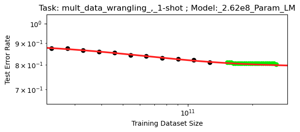
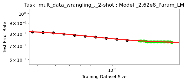
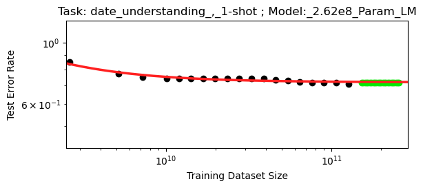
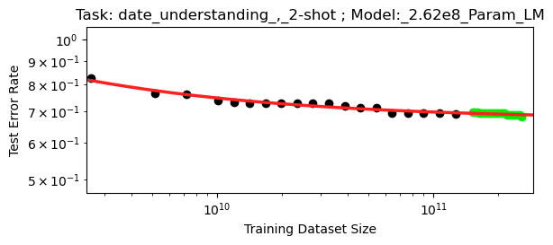
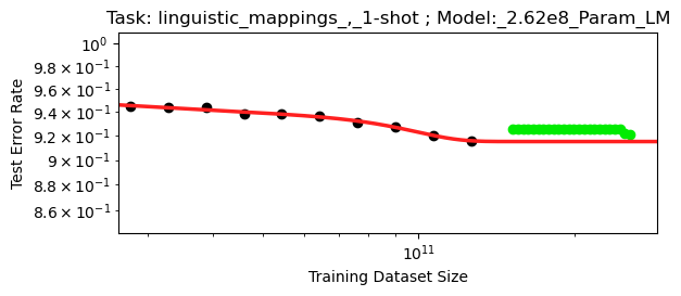
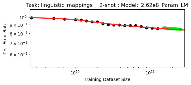
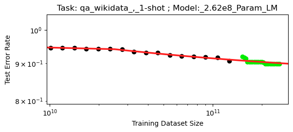
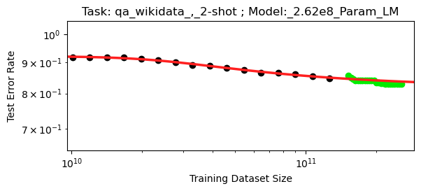
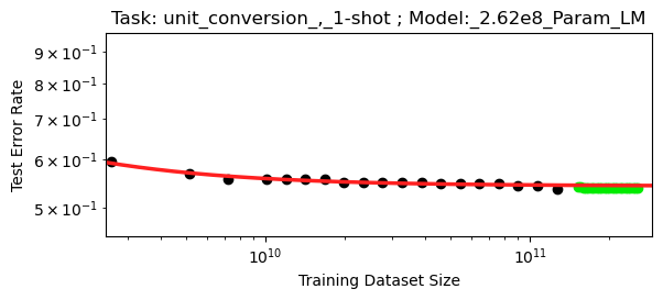
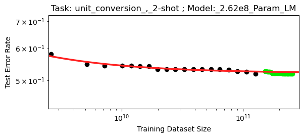
Figure 37: Extrapolation Results of BNSL on Downstream BIG-Bench (BB). X-axis is pretraining dataset size. See Section 5.2 for more details. From eyeballing, we think the subset of BIG-Bench with unsatisfactory extrapolations has unsatisfactory extrapolations due to the maximum (along the x-axis) of the black point used for fitting being near or before a break; this is accentuated by not having enough points for fitting for the SciPy fitter to be able to determine whether the break is an actual break or just noisy deviation. See Section 6 for more details on this explanation.

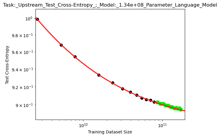
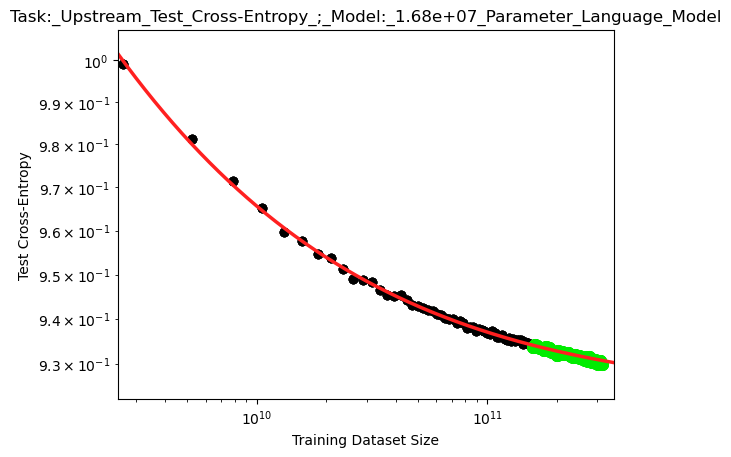
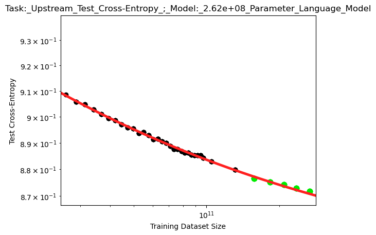
Figure 38: Extrapolation Results of BNSL on Language Modeling (LM). See Section 5.2 for more details.

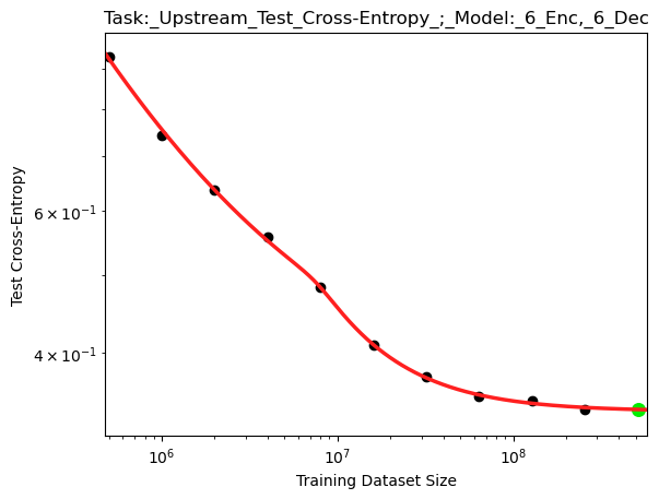
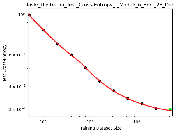
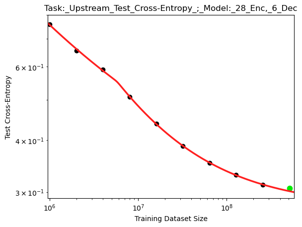
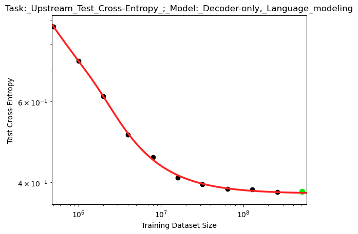
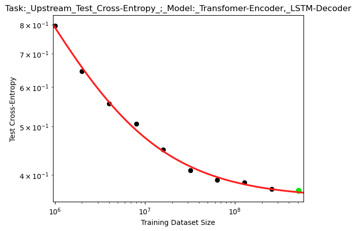
Figure 39: Extrapolation Results of BNSL on Neural Machine Translation (NMT). See Section 5.2 for more details.

To view all plots of the BNSL on each of these tasks, see Figures 37, 39, 38 in Appendix A.36. To view plots of M1, M2, M3, and M4 on these tasks, see Figure 8 of Alabdulmohsin et al. (2022).

In Section A.15 (and also Figure 2), we additionally show that BNSL yields accurate extrapolations of performance (to scales that are over an order of magnitude larger than the maximum (along the x-axis) of the points used for fitting) on large-scale downstream language tasks when number of model parameters is on the x-axis.

In Section A.18, we additionally show that BNSL accurately models and extrapolates the scaling behavior of sparse models (i.e. sparse, pruned models and sparsely gated mixture-of-expert models).

In Section A.16, BNSL accurately extrapolates the scaling behavior of retrieval-augmented models.

In Section A.17, BNSL accurately extrapolates the scaling behavior with input size (also know as input / context length) of the model on the x-axis.

In Section A.32, BNSL also accurately extrapolates the scaling behavior of recurrent neural nets.

In Section A.34, we additionally show that BNSL yields accurate extrapolations of performance on large-scale downstream audio (speech recognition) tasks.

In Section A.20, we show BNSL accurately models and extrapolates the scaling behavior with finetuning dataset size on the x-axis and the scaling behavior of computer programming / coding.

In Section A.21, we additionally show BNSL accurately models and extrapolates the scaling behavior of uncertainty estimation / calibration.

In Section A.28, BNSL accurately extrapolates the scaling behavior of tasks involving molecules.

In Section A.27, BNSL accurately extrapolates the scaling behavior of OOD detection.

In Section A.25, BNSL accurately extrapolates the scaling behavior of quantization.

In Section A.29, BNSL accurately extrapolates the scaling behavior of math word problems.

In Section A.26, BNSL accurately extrapolates the scaling behavior of distillation.

In Section A.35, BNSL accurately extrapolates the scaling behavior of downstream performance to scales that are over 100,000 times larger than the maximum (along x-axis) of the points used for fitting (and also when amount of compute used for (pre-)training is on the x-axis and compute is scaled in the manner that is Pareto optimal with respect to the downstream performance evaluation metric on the y-axis).

Domain	Task	Model		M1 $\downarrow$	M2 $\downarrow$	M3 $\downarrow$	M4 $\downarrow$	BNSL $\downarrow$
BB	date understanding, 1-shot	2.62e+8 Param		3.19e-2 ± 9.6e-4	3.19e-2 ± 9.6e-4	4.67e-3 ± 1.4e-4	3.19e-2 ± 9.6e-4	3.40e-3 ± 7.9e-5
BB	date understanding, 2-shot	2.62e+8 Param		2.86e-2 ± 6.2e-4	2.86e-2 ± 6.2e-4	4.83e-3 ± 4.1e-4	2.86e-2 ± 6.2e-4	4.38e-3 ± 4.0e-4
BB	linguistic mappings, 1-shot	2.62e+8 Param		1.66e-2 ± 5.5e-4	1.62e-2 ± 5.4e-4	1.66e-2 ± 5.5e-4	1.33e-2 ± 3.8e-4	1.13e-2 ± 2.2e-4
BB	linguistic mappings, 2-shot	2.62e+8 Param		1.70e-2 ± 6.5e-4	1.70e-2 ± 6.5e-4	1.70e-2 ± 6.5e-4	1.06e-2 ± 5.1e-4	9.51e-3 ± 5.1e-4
BB	mult data wrangling, 1-shot	2.62e+8 Param		1.07e-2 ± 1.0e-3	1.07e-2 ± 1.0e-3	1.07e-2 ± 1.0e-3	6.66e-3 ± 7.3e-4	6.39e-3 ± 4.6e-4
BB	mult data wrangling, 2-shot	2.62e+8 Param		1.57e-2 ± 1.5e-3	1.57e-2 ± 1.5e-3	1.57e-2 ± 1.5e-3	5.79e-3 ± 7.0e-4	2.67e-3 ± 2.7e-4
BB	qa wikidata, 1-shot	2.62e+8 Param		4.27e-3 ± 8.9e-4	4.32e-3 ± 8.2e-4	4.27e-3 ± 8.9e-4	4.32e-3 ± 8.2e-4	4.68e-3 ± 7.3e-4
BB	qa wikidata, 2-shot	2.62e+8 Param		4.39e-3 ± 7.0e-4	4.66e-3 ± 6.4e-4	4.39e-3 ± 7.0e-4	9.02e-3 ± 6.9e-4	8.05e-3 ± 7.3e-4
BB	unit conversion, 1-shot	2.62e+8 Param		8.30e-3 ± 4.4e-4	8.30e-3 ± 4.4e-4	1.48e-3 ± 2.7e-4	4.79e-3 ± 3.4e-4	1.07e-2 ± 2.5e-4
BB	unit conversion, 2-shot	2.62e+8 Param		1.07e-2 ± 4.4e-4	1.07e-2 ± 4.4e-4	7.50e-3 ± 5.5e-4	7.55e-3 ± 5.1e-4	7.02e-3 ± 3.9e-4
LM	upstream test cross-entropy	1.07e+9 Param		1.71e-2 ± 6.0e-4	1.66e-3 ± 5.1e-5	4.50e-3 ± 5.9e-5	1.28e-3 ± 3.9e-5	9.71e-4 ± 3.2e-5
LM	upstream test cross-entropy	4.53e+8 Param		1.65e-2 ± 6.6e-4	7.41e-4 ± 9.8e-5	6.58e-4 ± 6.6e-5	7.41e-4 ± 9.8e-5	5.86e-4 ± 7.7e-5
LM	upstream test cross-entropy	2.62e+8 Param		1.55e-2 ± 7.2e-4	9.20e-4 ± 9.7e-5	3.97e-3 ± 1.3e-4	9.20e-4 ± 9.7e-5	7.90e-4 ± 5.1e-5
LM	upstream test cross-entropy	1.34e+8 Param		1.43e-2 ± 4.8e-4	1.46e-3 ± 6.8e-5	6.46e-4 ± 5.1e-5	1.46e-3 ± 6.8e-5	9.01e-4 ± 5.5e-5
LM	upstream test cross-entropy	1.68e+7 Param		6.37e-3 ± 9.4e-5	3.03e-4 ± 1.2e-5	1.56e-3 ± 3.5e-5	3.03e-4 ± 1.2e-5	4.34e-4 ± 1.8e-5
NMT	upstream test cross-entropy	28 Enc, 6 Dec		1.71e-1 ± 0	5.64e-2 ± 0	3.37e-2 ± 0	1.81e-2 ± 0	1.69e-2 ± 0
NMT	upstream test cross-entropy	6 Enc, 28 Dec		2.34e-1 ± 0	5.27e-2 ± 0	1.65e-2 ± 0	4.44e-2 ± 0	1.56e-2 ± 0
NMT	upstream test cross-entropy	6 Enc, 6 Dec		2.62e-1 ± 0	3.84e-2 ± 0	8.92e-2 ± 0	2.05e-2 ± 0	1.37e-3 ± 0
NMT	upstream test cross-entropy	Dec-only, LM		2.52e-1 ± 0	1.03e-2 ± 0	3.28e-2 ± 0	8.43e-3 ± 0	7.33e-3 ± 0
NMT	upstream test cross-entropy	Transformer-Enc, LSTM-Dec		1.90e-1 ± 0	1.26e-2 ± 0	6.32e-2 ± 0	1.26e-2 ± 0	8.30e-3 ± 0

Table 4: Extrapolation Results on scaling behavior of Language Tasks (Downstream and Upstream). See Section 5.2 for more details. Numbers for M1, M2, M3, and M4 were obtained via correspondence with authors of Alabdulmohsin et al. (2022). BB stands for BIG-Bench (Srivastava et al., 2022). NMT stands for Neural Machine Translation. LM stands for Language Modeling.

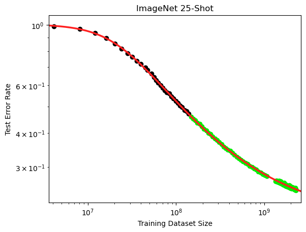
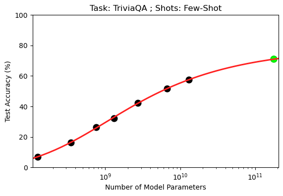
Figure 2: BNSL accurately Extrapolating Downstream Performance to Scales that are greater than an Order of Magnitude larger than the maximum (along the x-axis) of the points used for fitting; there are additional similar results in the Appendix. Experimental data of scaling behavior in top plot obtained from scaling laws benchmark of Alabdulmohsin et al. (2022); see Appendix A.8 for more details. Experimental data of scaling behavior in bottom plot obtained from Table H.1 of GPT-3 arXiv paper (Brown et al., 2020); see Appendix A.15 for more details.

5.3 Reinforcement Learning

We show that BNSL accurately models and extrapolates the scaling behaviors of various multi-agent and single-agent reinforcement learning algorithms trained in various environments. In the top left plot and top middle plot and top right plot of Figure 3, BNSL accurately models and extrapolates the scaling behavior of the AlphaZero algorithm (Silver et al., 2017) trained to play the game Connect Four from Figure 4 and Figure 5 and Figure 3 respectively of Neumann & Gros (2022); the x-axes respectively are compute (FLOPs) used for training, training dataset size (states), and number of model parameters. In Figure 3 bottom left and bottom right respectively, BNSL accurately models and extrapolates the scaling behavior of the Phasic Policy Gradient (PPG) algorithm (Cobbe et al., 2021b) trained to play the Procgen (Cobbe et al., 2020) game called StarPilot and the scaling behavior of the Proximal Policy Optimization (PPO) algorithm (Schulman et al., 2017) trained to play the Procgen (Cobbe et al., 2020) game called Heist.
In Section A.31, we additionally find BNSL accurately extrapolates the scaling behavior with amount of test-time (a.k.a. inference) compute (available to the agent) on the x-axis.
In Section A.22, we additionally find BNSL accurately extrapolates the scaling behavior of a pretrained language model finetuned (i.e. aligned) via Reinforcement Learning from Human Feedback (RLHF) to be helpful from Figure 1 of Bai et al. (2022).

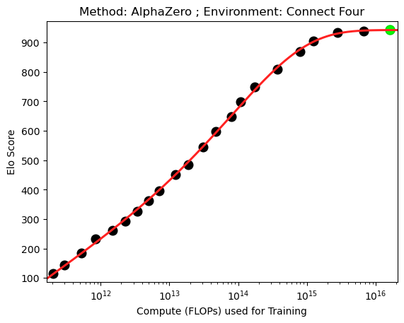
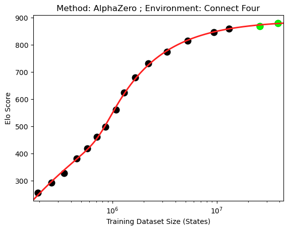
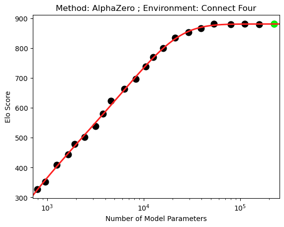
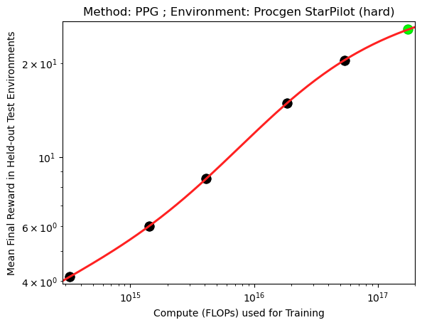
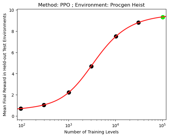
Figure 3: Extrapolation Results of BNSL on Reinforcement Learning Scaling Experimental Data. Experimental data of the top left plot and top middle plot and top right plot is from Figure 4 and Figure 5 and Figure 3 respectively of Neumann & Gros (2022). Experimental Data of the bottom left plot is from Figure 1 left of Hilton et al. (2023). Experimental Data of the bottom right plot is from Figure 2 of Cobbe et al. (2020). Top left and bottom left plot is the compute-optimal Pareto frontier. See Section 5.3 for more details.

5.4 Non-Monotonic Scaling

We show that BNSL accurately models and extrapolates non-monotonic scaling behaviors such as those that are exhibited by Transformers (Vaswani et al. (2017)) during double descent (Nakkiran et al., 2021) in Figure 4. Various other functional forms are mathematically incapable of expressing non-monotonic behaviors (as shown in Section 4).

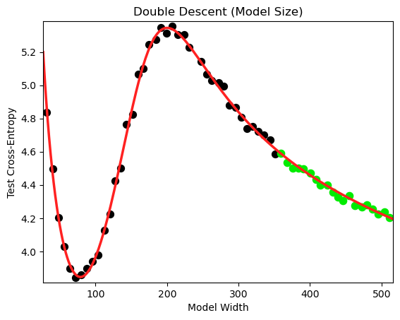
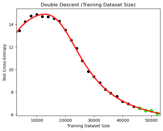
Figure 4: Extrapolation Results of BNSL on Double Descent. Both plots are of transformers trained to do neural machine translation via minimizing cross-entropy. Experimental data of left figure is obtained from Figure 8 top of Nakkiran et al. (2021); “Model Width” on the x-axis refers to embedding dimension $d_{model}$ of the transformer; note that model width is linearly proportional to number of model parameters, so number of model parameters on the x-axis would yield same results. Experimental data of the right figure is obtained from Figure 11b of Nakkiran et al. (2021). The plot on the left contains two breaks of a BNSL fit to the black points. See Section 5.4 for more details.

5.5 Inflection Points

We show that BNSL accurately models and extrapolates the scaling behavior of tasks that have an inflection point on a linear-linear plot such as the task of arithmetic (4-digit addition). Here we model and extrapolate the scaling behavior of a transformer model (Vaswani et al. (2017)) with respect to the training dataset size on the 4-digit addition task. Various other functional forms are mathematically incapable of expressing inflection points on a linear-linear plot (as shown in Section 4) and as a result, are mathematically incapable of expressing and modeling inflection points (on a linear-linear plot) that are present in the scaling behavior of 4-digit addition. In Figure 5 left, we show that BNSL expresses and accurately models the inflection point present in the scaling behavior of 4-digit addition and as a result accurately extrapolates the scaling behavior of 4-digit addition. For more details about the hyperparameters, see Appendix A.5.
Also, in Section A.10 we additionally find that BNSL accurately models and extrapolates the scaling behavior with number of training steps on the x-axis.
Also, in Section A.26 and the bottom left plot of Figure 16 of Section A.18 we additionally find that BNSL accurately models and extrapolates the scaling behavior of tasks that have an inflection point on a linear-linear plot when number of models parameters is on the x-axis.

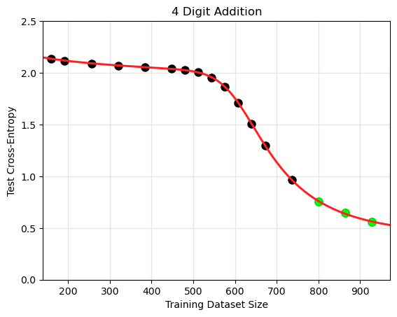
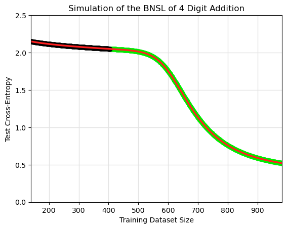
Figure 5: Extrapolation of BNSL on 4-Digit Addition. Note these plots are linear-linear. Each point in left plot is mean of greater than 1000 seeds at that dataset size. In left plot, each point is gathered from a model trained to do task of 4-digit addition. In right plot, each point is gathered from a noiseless simulation of the BNSL of the task of 4-digit addition. See Sections 5.5, A.5, 6, for more details.

6 The Limit of the Predictability of Scaling Behavior

We use BNSL to glean insights about the limit of the predictability of scaling behavior. Recent papers (Ganguli et al., 2022; Wei et al., 2022a; Srivastava et al., 2022) have advertised many tasks as having “emergent” “breakthrough” “phase transition/change/shift” scaling behaviors. We define all these quoted phrases as any scaling behaviors with greater than $0$ breaks (e.g. $\sim$all the plots in this paper and the appendix due to the fact that 100% of plots in this paper and the appendix contain the region(s) surrounding (or neighboring) $\geq$1 break(s) of a BNSL fit to black points). The most extreme of these scaling behaviors are those in which it is simultaneously true that $|c_{i>0}|$ is large and $f_{i}$ is small (and nonnegative); one such example is the task of 4-digit addition (there are other such tasks in the appendix). In the previous section and in Figure 5 left, we successfully predicted (i.e. extrapolated) the scaling behavior of 4-digit addition (arithmetic). However, we are only able to accurately extrapolate the scaling behavior if given some points from training runs with a training dataset size of at least 720, and the break in which the scaling behavior of 4-digit addition transitions from one power law to another steeper power-law happens at around training dataset size of 415.

Ideally, one would like to be able to extrapolate the entire scaling behavior by fitting only points from before the break. In Figure 5 right, we use a noiseless simulation of the BNSL of 4-digit addition to show what would happen if one had infinitely many training runs / seeds to average out all the noisy deviation between runs such that one could recover (i.e. learn via a curve-fitting library such as SciPy (Virtanen et al., 2020)) the learned constants of the BNSL as well as possible. When using this noiseless simulation, we find that we are only able to accurately extrapolate the scaling behavior if given some points from training runs with a training dataset size of at least 415, which is very close to the break.

This has a few implications:

1) When the scaling behavior exhibits greater than 0 breaks that are sufficiently sharp, there is a limit as to how small the maximum (along the x-axis) of the points used for fitting can be if one wants to perfectly extrapolate the scaling behavior, even if one has infinitely many seeds / training runs.

2) If an additional break of sufficient sharpness happens at a scale that is sufficiently larger than the maximum (along the x-axis) of the points used for fitting, there does not (currently) exist a way to extrapolate the scaling behavior after that additional break.

3) If a break of sufficient sharpness happens at a scale sufficiently smaller than the maximum (along the x-axis) of the points used for fitting, points smaller (along the x-axis) than that break can often be useless for improving extrapolation. See Appendix A.7 for examples of scenarios in which points smaller (along the x-axis) than that break do improve extrapolation.

7 Discussion

We have presented a smoothly broken power law functional form that accurately models & extrapolates the scaling behaviors of artificial neural networks for various architectures & for each of various tasks from a very large & diverse set of upstream & downstream tasks. This set includes large-scale vision, language, audio, video, diffusion, generative modeling, multimodal learning, contrastive learning, AI alignment, AI capabilities, robotics, out-of-distribution generalization, continual learning, transfer learning, uncertainty estimation / calibration, out-of-distribution detection, adversarial robustness, distillation, sparsity, retrieval, quantization, pruning, fairness, molecules, computer programming/coding, math word problems, “emergent” “phase transitions”, arithmetic, supervised learning, unsupervised/self-supervised learning, & reinforcement learning (single agent & multi-agent). The architectures in this set include ResNets, Transformers, MLPs, MLP-Mixers, RNNs, GNNs, U-Nets, Ensembles (& Non-Ensembles), MoE (& Non-MoE) models, & Sparse Pruned (& Non-Sparse Unpruned) models. When compared to other functional forms for neural scaling behavior, this functional form yields extrapolations of scaling behavior that are considerably more accurate on this set. Additionally, this functional form accurately models & extrapolates scaling behavior that other functional forms are incapable of expressing such as the non-monotonic transitions present in the scaling behavior of phenomena such as double descent & the delayed, sharp inflection points present in the scaling behavior of tasks such as arithmetic. Lastly, we used this functional form to glean insights about the limit of the predictability of scaling behavior.

Ethics Statement

We place relatively high probability on the claim that variants of smoothly broken power laws perhaps are the “true” functional form of the scaling behavior of many (all?) things that involve artificial neural networks. Due to the fact that BNSL is a variant of smoothly broken power laws, an ethical concern one might have about our work is that revealing BNSL might differentially (Hendrycks & Mazeika, 2022) improve A(G)I capabilities progress relative to A(G)I safety/alignment progress. A counter-argument is that BNSL will also allow the A(G)I safety/alignment field to extrapolate the scaling behaviors of its methods for aligning A(G)I systems and as a result will also accelerate alignment/safety progress. Existing scaling laws besides BNSL struggle especially to model downstream performance, e.g. on safety-relevant evaluations (especially evaluations (such as interpretability and controllability) that might exhibit non-monotonic scaling behavior in the larger scale systems of the future); we believe our work could differentially help in forecasting emergence of novel capabilities (such as reasoning (Wei et al., 2022b)) or behaviors (such as deception or dishonesty (Evans et al., 2021; Lin et al., 2021)), and thus help avoid unpleasant surprises.

A potential limitation of the current approach is the need to collect enough samples of the system’s performance (i.e. the (x,y) points required for estimating the scaling law’s parameters). A small number of samples sometimes may not be sufficient to accurately fit and extrapolate the BNSL functional form, and obtaining a large number of such samples can sometimes be costly. This has the ethical implication that entities with more compute to gather more points maybe will have considerably more accurate extrapolations of scaling behavior than entities with less compute. As a result, entities with less compute (e.g. academia) maybe will have less foresight than entities with more compute (e.g. Big Tech), which could maybe exacerbate the gap between entities with more compute (e.g. Big Tech) and entities with less compute (e.g. academia).

Acknowledgments

We are thankful for useful feedback and assistance from Kartik Ahuja, Ibrahim Alabdulmohsin, Ankesh Anand, Jacob Buckman, Guillaume Dumas, Leo Gao, Andy Jones, Neel Nanda, Behnam Neyshabur, Gabriel Prato, Stephen Roller, Michael Trazzi, Tony Wu and others.

Appendix A Appendix

A.1 Analysis and Explanation of why BNSL is smoothly connected piecewise (approximately) linear function on a log-log plot

Analysing Equation 1 reveals why BNSL is smoothly connected piecewise (approximately) linear function on a log-log plot. Considering $y$ as a function of $z:=\log(x)$, applying logarithms to both sides and setting $a=0$ yields:

$$\log(y)=\log(b)-c_{0}z-\sum_{i=1}^{n}c_{i}f_{i}\log\left(1+\left(\frac{\exp(z)}{d_{i}}\right)^{1/f_{i}}\right).$$ (3)

We can now see the terms in the sum resemble the well-known $\mathrm{softplus}$ function: $\mathrm{softplus}(x):=\log(1+exp(x))$, which smoothly interpolates between the constant 0 function and the identity. By plotting one such term for different values of $c_{i},d_{i},f_{i}$, it is easy to confirm that they influence the shape of the curve as described in Section 2.

A.2 Decomposition of Broken Neural Scaling Law into power law segments that it is composed of

We now show a way to decompose a BNSL (Equation 1) with 3 breaks into the power law segments that it is composed of. This decomposition is what we used to produce power law segments 1-4 overlaid in Figure 1 and is usable when values of $f$ in Equation 1 are not too large and $a$ is subtracted out from right-hand side of Equation 1. This decomposition pattern is straight-forward to extend to $n$ breaks.

$segment_{1}=b*(x)^{-(c_{0})}$

$segment_{2}=b*(d_{1})^{-(c_{0})}*(x\hskip 3.98337pt/d_{1})^{-(c_{1}+c_{0})}$

$segment_{3}=b*(d_{1})^{-(c_{0})}*(d_{2}/d_{1})^{-(c_{1}+c_{0})}*(x\hskip 3.98337pt/d_{2})^{-(c_{2}+c_{1}+c_{0})}$

$segment_{4}=b*(d_{1})^{-(c_{0})}*(d_{2}/d_{1})^{-(c_{1}+c_{0})}*(d_{3}/d_{2})^{-(c_{2}+c_{1}+c_{0})}*(x\hskip 3.98337pt/d_{3})^{-(c_{3}+c_{2}+c_{1}+c_{0})}$

A.3 Definition of Root Mean Squared Log Error

$$Root\_Mean\_Squared\_Log\_Error=RMSLE=\sqrt{(\sum_{i=1}^{N}(log(y_{i})-log(\hat{y}_{i}))^{2})/N}$$

A.4 Definition of Root Standard Log Error

$$error=(log(y_{i})-log(\hat{y}_{i}))^{2})$$

$$\mu_{error}=\frac{1}{N}\sum_{i=1}^{N}error$$

$$\sigma_{error}=\sqrt{\frac{1}{N-1}\sum_{i=1}^{N}(error_{i}-\mu_{error})^{2}}$$

$$Root\_Standard\_Log\_Error=\sqrt{\mu_{error}+\frac{\sigma_{error}}{\sqrt{len(\hat{y})}}}-\sqrt{\mu_{error}}$$

A.5 Experimental details of Sections 5.5 and A.10

We perform an extensive set of experiments to model and extrapolate the scaling behavior for the 4-digit arithmetic addition task with respect to the training dataset size. Our code is based on the minGPT implementation (Karpathy, 2020). We set the batch size equal to the training dataset size. We do not use dropout nor a learning rate decay / schedule / warmup here. Each experiment was run on a single V100 GPU and each run took less than 2 hours. For our experiments we train the transformer model using the following set of hyperparameters:

$D_{model}$	128
$D_{MLP}$	512
Number of heads	2
Number of transformer blocks	1
Learning rate	0.0001
Weight Decay	0.1
Dropout Probability	0.0
Optimizer	Adam
Adam beta 1	0.9
Adam beta 2	0.95
Adam epsilon	$10^{-8}$
Gradient Norm Clip Threshold	1.0
Dataset sizes	144-1008
Vocab Size	10

Table 5: Hyperparameters for 4-digit addition task

A.6 Experimental details of fitting BNSL and determining the number of breaks

We fit BNSL as follows: We first use scipy.optimize.brute to do a grid search of the values of the constants ($a,b,c_{0},c_{1}...c_{n},d_{1}...d_{n},f_{1}...f_{n}$) of BNSL that best minimize the mean squared log error (MSLE) between the real data and the output of BNSL. We then use the values obtained from the grid search as the initialization of the non-linear least squares algorithm of scipy.optimize.curve_fit. We then use the non-linear least squares algorithm of scipy.optimize.curve_fit to minimize the mean squared log error (MSLE) between the real data and the output of BNSL.

The version of MSLE we use for such optimization is the following numerically stable variant:

$$Numerically\_Stable\_MSLE=\sum_{i=1}^{N}((log(y_{i}+1)-log(\hat{y}_{i}+1))^{2})/N$$

With regards to determining the number of breaks $n$ in the BNSL, one way to go about doing so is to hold out the last few largest (along the x-axis) points used for fitting (not the green points used for evaluating extrapolation) as a validation set. The value of $n$ with lowest validation error when fitting on the remaining smaller (along the x-axis) points is then used. As mentioned in implication 3 of Section 6, there are many scenarios in which a break of sufficient sharpness happens at a scale sufficiently smaller than the maximum (along the x-axis) of the points used for fitting such that points smaller (along the x-axis) than that break can often be useless for improving extrapolation. For example, if a full scaling behavior contains a very sharp break and then a very smooth break, one can crop out the smaller (along the x-axis) points that contain the sharp break and fit a BNSL with a single break (i.e. with $n=1$) if one only cares about extrapolation accuracy. To determine where the crop point is, one can employ the same validation set strategy mentioned at the beginning of this paragraph, but selecting for crop point instead of number of breaks. One reason why someone may want to use the strategies mentioned throughout this paragraph is that sometimes the value(s) of $|c_{i>0}|$ can be small such that it is hard for humans to identify the break(s) via eyeballing.

A.7 Examples in which fitting points before a break improves extrapolation even though the maximum (along the x-axis) of the points used for fitting is larger (along the x-axis) than that break

There are examples in the appendix (e.g. one example is in Figure 24 of Appendix A.26) in which BNSL accurately models and accurately extrapolates scaling behaviors in which the points used for fitting contain only one point that is larger (along the x-axis) than the largest break. In such examples, it is impossible to accurately extrapolate the scaling behavior using only points after that break because a scaling behavior is unidentifiable if one can only use a single point for fitting. In such examples, BNSL accurately integrates information from before that break to obtain accurate extrapolation.

A.8 Extrapolation to Scales that are over an Order of Magnitude larger than the maximum (along the x-axis) of the points used for fitting

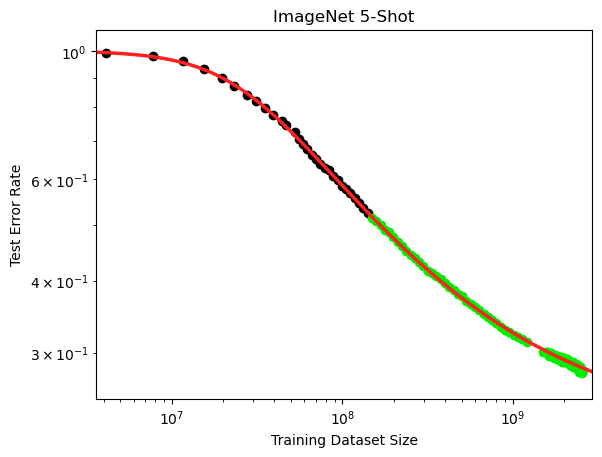
Figure 6: Extrapolation Results of BNSL to Scales that are over an Order of Magnitude larger than the maximum (along the x-axis) of the points used for fitting. Experimental data of scaling behavior obtained from scaling laws benchmark of Alabdulmohsin et al. (2022). The upstream task is supervised pretraining of MLP mixers (MiX) (Tolstikhin et al., 2021) on subsets (i.e. the x-axis of plot) of JFT-300M (Sun et al., 2017). The Downstream Task is n-shot ImageNet classification (i.e. the y-axis of plot). See Section A.8 for more details.

In Figure 6, we show that BNSL accurately extrapolates to scales that are over an order of magnitude larger than the maximum (along the x-axis) of the points used for fitting. The upstream task is supervised pretraining of MLP mixers (MiX) (Tolstikhin et al., 2021) on subsets (i.e. the x-axis of plot) of JFT-300M (Sun et al., 2017). The downstream task is n-shot ImageNet classification (i.e. the y-axis of plot). The experimental data of this scaling behavior is obtained from Alabdulmohsin et al. (2022).

A.9 Extrapolation Results for Downstream Vision Tasks when training runs are scaled to be compute-optimal (and amount of compute used for (pre-)training is on the x-axis).

Task	Model	M3 $\downarrow$	BNSL $\downarrow$
ImageNet 10-Shot	ViT	1.47e-2 ± 6.61e-3	8.84e-3 ± 5.08e-3
ImageNet Finetune	ViT	5.71e-3 ± 3.42e-3	5.44e-3 ± 3.52e-3

Table 6: Extrapolation Results for Downstream Vision Tasks when training runs are scaled using the compute-optimal scaling (i.e. Pareto frontier) with respect to downstream performance (and amount of compute used for (pre-)training is on the x-axis). Experimental data obtained from Figure 2 of Zhai et al. (2021). See Section A.9 for more details.

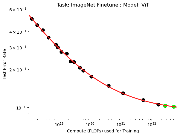
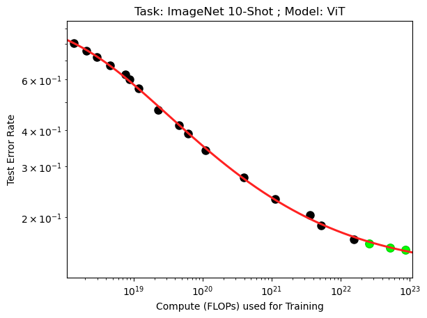
Figure 7: Extrapolation Results of BNSL for Downstream Vision Tasks when training runs are scaled to be compute-optimal (and amount of compute used for (pre-)training is on the x-axis). Experimental data obtained from Figure 2 of Zhai et al. (2021). See Section A.9 for more details.

In Figure 7 via fitting BNSL, we additionally obtain accurate extrapolations of the scaling behavior of large-scale downstream vision tasks when compute (FLOPs) used for (pre-)training is on the x-axis and compute is scaled in the manner that is Pareto optimal with respect to the performance evaluation metric (downstream accuracy in this case). The y-axis is downstream test error rate on ImageNet. The upstream task is supervised pretraining of ViT (Dosovitskiy et al., 2020) models on subsets of JFT-300M (Sun et al., 2017). The experimental scaling data was obtained from Figure 2 of Zhai et al. (2021), and as a result in Table 6 we compare extrapolation of BNSL to the extrapolation of M3 (which was proposed in Zhai et al. (2021)); we find that BNSL yields extrapolations of scaling behavior that are more accurate (i.e. have lower RMSLE) on these tasks.

A.10 Extrapolation Results with Number of Training Steps on the x-axis

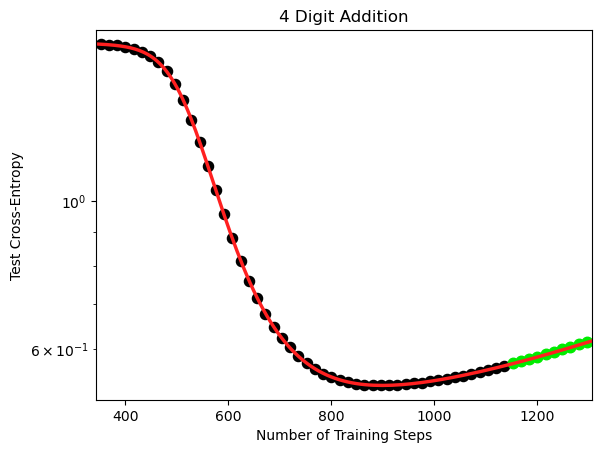
Figure 8: Extrapolation Results of BNSL with Number of Training Steps on the x-axis. The y-axis is Test Cross-Entropy. The x-axis is the number of training steps. Each point is the mean of greater than 600 seeds at that number of training steps. The training dataset size is 992. All hyperparameters and experimental details are described in Section A.5. The task is 4-digit addition. This plot contains two breaks of a BNSL fit to the black points. See Section A.10 for more details.

In Figure 8, we find BNSL accurately extrapolates the scaling behavior with number of training steps on the x-axis.

A.11 Extrapolation Results for Diffusion Generative Models of Images

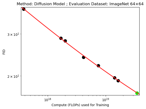
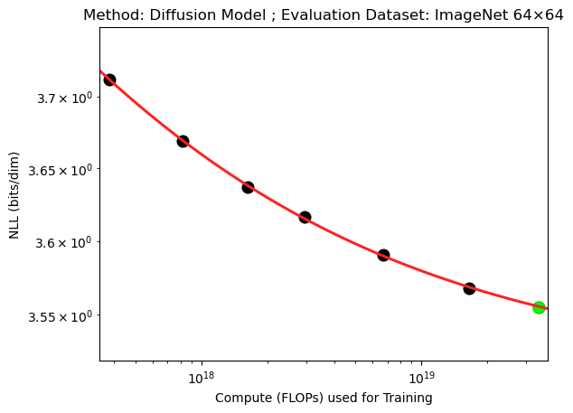
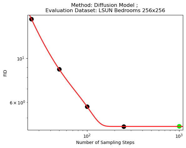
Figure 9: Extrapolation Results of BNSL for scaling behavior of Diffusion Generative Models of Images. Frechet Inception Distance (FID) score is on the y-axis in the left plot and bottom plot. Test Negative Log-Likelihood (NLL) is on the y-axis in the right plot. For top plots, Imagenet 64x64 is the evaluation dataset, compute used for training is on the x-axis, and compute is scaled in the manner that is Pareto optimal with respect to the performance evaluation metric on the y-axis. For bottom plot, LSUN Bedrooms 256x256 is the evaluation dataset, and the number of sampling steps is on the x-axis. Experimental data of top plots obtained from Figure 10 of Nichol & Dhariwal (2021). Experimental data of bottom plot obtained from the “$L_{hybrid}$ (batch=128, lr=1e-4)” results of Figure 11 of Nichol & Dhariwal (2021). See Section A.11 for more details.

In Fig. 9, BNSL accurately extrapolates the scaling behavior of Diffusion Generative Image Models.

A.12 Extrapolation Results for Generative Models of Video

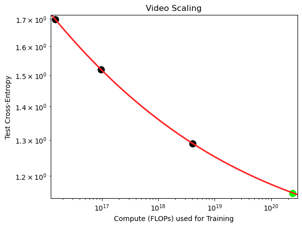
Figure 10: Extrapolation Results of BNSL for scaling behavior of Generative Models of Video. Upstream Test Cross-Entropy is on the y-axis. During training, compute (used for training autoregressive transformer) on the x-axis is scaled in the manner that is Pareto optimal with respect to the performance evaluation metric on the y-axis. Experimental data of scaling behavior obtained from top right plot of Figure 5 of Henighan et al. (2020). See Section A.12 for more details.

In Figure 10, we show that BNSL accurately extrapolates the scaling behavior of generative models of video. Each frame is downsampled to a pixel resolution of 64x64; each frame is then tokenized via a pretrained 16x16 VQVAE (Van Den Oord et al., 2017) to obtain 256 tokens per frame. 16 consecutive frames are then input to an autoregressive transformer as a length 4096 (16x16x16) sequence. The training dataset (& testing dataset) is from 100 hours of videos scraped from the web.

A.13 Extrapolation Results when Data is Pruned Pareto Optimally

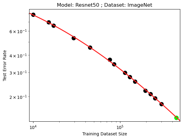
Figure 11: Extrapolation Results of BNSL for scaling behavior when data is pruned Pareto optimally (such that each point along the x-axis uses the subset of the dataset that yields the best performance (y-axis value) for that dataset size (x-axis value)). Experimental data of scaling behavior obtained from Figure 3D of Sorscher et al. (2022). See Section A.13 for more details.

In Figure 11, we show that BNSL accurately extrapolates the scaling behavior when data is pruned Pareto optimally (such that each point along the x-axis uses the subset of the dataset that yields the best performance (y-axis value) for that dataset size (x-axis value)) from Figure 3D of Sorscher et al. (2022).

A.14 Extrapolation Results when Upstream Performance is on the x-axis

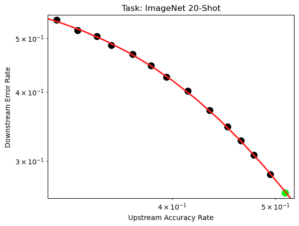
Figure 12: Extrapolation Results of BNSL for scaling behavior when Upstream Performance is on the x-axis and Downstream Performance is on the y-axis. Experimental data of scaling behavior obtained from Figure 5 of Abnar et al. (2021). The upstream task is supervised pretraining of ViT (Dosovitskiy et al., 2020) on subsets of JFT-300M (Sun et al., 2017). The Downstream Task is 20-shot ImageNet classification. See Section A.14 for more details.

In Figure 12, we show that BNSL accurately extrapolates the scaling behavior when upstream performance is on the x-axis and downstream performance is on the y-axis. The upstream task is supervised pretraining of ViT (Dosovitskiy et al., 2020) on subsets of JFT-300M (Sun et al., 2017). The downstream task is 20-shot ImageNet classification. The experimental data of this scaling behavior is obtained from Figure 5 of Abnar et al. (2021).

A.15 Extrapolation Results for Downstream Language Tasks when Number of Model Parameters is on the x-axis.
These extrapolations are to scales over an order of magnitude larger than the maximum (along the x-axis) of the points used for fitting.

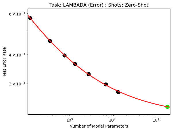
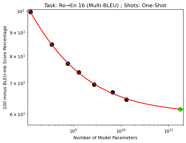
Figure 13: Extrapolation Results of BNSL for Downstream Language Tasks when Number of Model Parameters is on the x-axis. Note that the held-out point(s) are over an order of magnitude larger than the maximum (along the x-axis) of the points used for fitting. “Few-Shot” in plot title means few-shot prompting is used (and “One-Shot” in plot title means one-shot prompting is used) for that downstream evaluation as described in GPT-3 arXiv paper (Brown et al., 2020). Experimental data obtained from Table H.1 of the GPT-3 arXiv paper (Brown et al., 2020). See Section A.15 for more details.

We find in general for each of every modality that the variance between seeds is higher when number of model parameters is on x-axis (as opposed to e.g. training dataset size on the x-axis). Table H.1 of the GPT-3 arXiv paper (Brown et al., 2020) release includes results for 8 numbers of model parameters. In Figure 13, we include examples of when 8 numbers of model parameters (7 for fitting, and largest held-out to evaluate extrapolation) are sufficient for obtaining accurate downstream extrapolation from BNSL due to variance between seeds being low enough. For many other downstream tasks with number of model parameters on the x-axis, the variance between seeds is much higher such that a number considerably larger than 7 points along the curve is needed to obtain an accurate extrapolation.

A.16 Extrapolation Results for Retrieval-Augmented Models

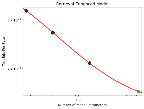
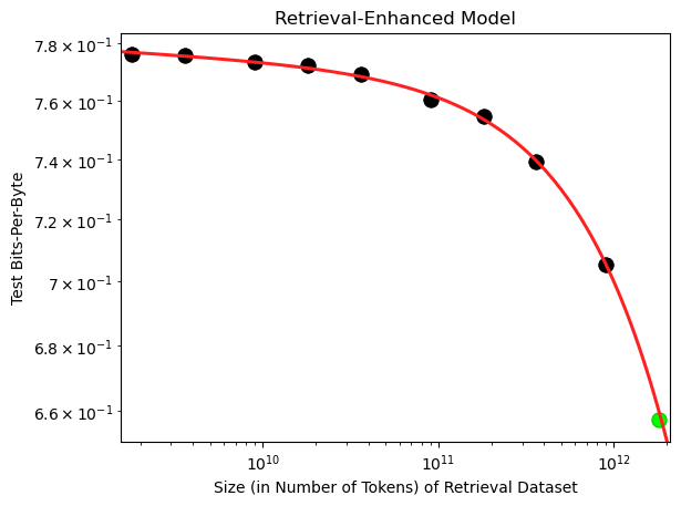
Figure 14: Extrapolation Results of BNSL for Retrieval-Augmented Models. Experimental data of left figure obtained from “RETRO [ON]” results of Figure 1 left of Borgeaud et al. (2022). Experimental data of right figure obtained from the 7.5 billion parameter model results of Figure 1 middle of Borgeaud et al. (2022). The y-axes are Zero-Shot Test Bits-per-Byte on Downstream C4 (Raffel et al., 2019) dataset. In left figure, x-axis is number of model parameters. In right figure, x-axis notably is Size (in Number of Tokens) of the Retrieval Dataset. See Section A.16 for more details.

In Figure 14, we find BNSL accurately extrapolates the scaling behavior (even downstream) of models augmented with a mechanism to retrieve data from a very large collection of data. In right plot of Figure 14, x-axis notably is Size (in Number of Tokens) of the Retrieval Dataset.

A.17 Extrapolation Results with Input Length (of the Model) on the x-axis

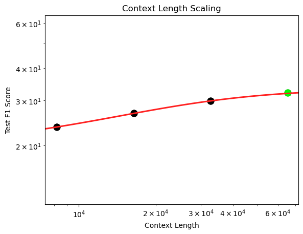
Figure 15: Extrapolation Results of BNSL for Input Size (also known as context length) of the model increases. Experimental data of obtained from the CoLT5 results of Figure 4 of Ainslie et al. (2023). The y-axis is Test F1 Score on Downstream NarrativeQA (Kočiskỳ et al., 2018) dataset. The x-axis is the context length (the four context length values are 8192, 16384, 32768, and 65536). See Section A.17 for more details.

In Figure 15, we find BNSL accurately extrapolates the scaling behavior (even downstream) with input size (also known as context length) (of the model) on the x-axis.

A.18 Extrapolation Results for Sparse Models

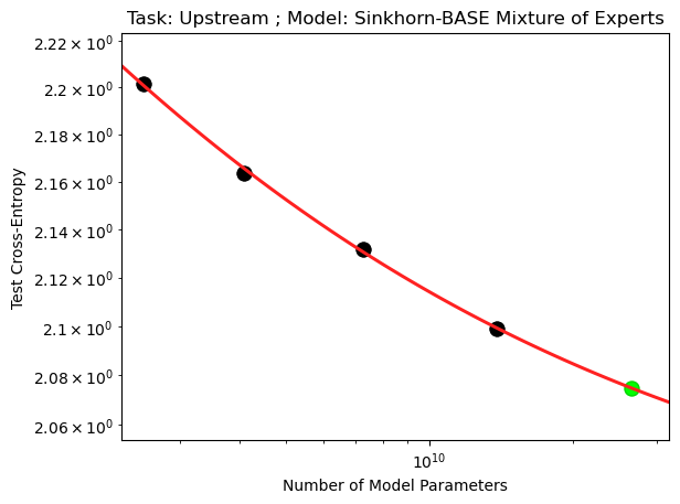
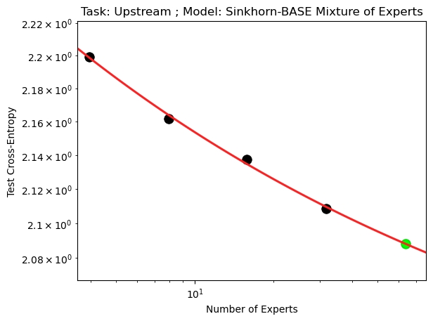
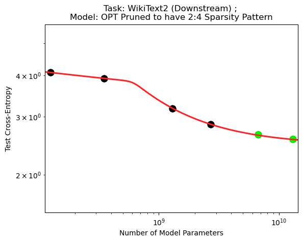
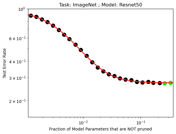
Figure 16: Extrapolation Results of BNSL for Sparse Models. Experimental data of top 2 figures are obtained from Figure 22 of Clark et al. (2022). Experimental data of bottom left figure obtained from Figure 1 right of Frantar & Alistarh (2023). Experimental data of bottom right figure obtained from the “n = 1/4” results of Figure 10 right of arXiv version of Rosenfeld et al. (2021). For all plots on the left, x-axis is number of model parameters that the model contains. In bottom left plot, the fraction of model parameters that have been pruned is held constant. In bottom right plot, x-axis is the fraction of model parameters that are not pruned. See Section A.18 for more details.

In Figure 16, we find BNSL accurately extrapolates the scaling behavior of sparse models (i.e. sparse, pruned models (bottom 2 plots) & sparsely gated mixture-of-expert models (top 2 plots)).

A.19 Extrapolation Results for Adversarial Robustness

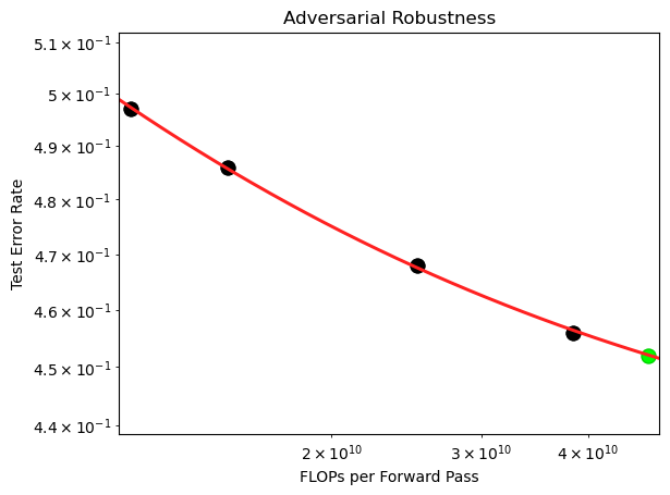
Figure 17: Extrapolation Results of BNSL for Adversarial Robustness. Test Error Rate is on the y-axis. FLOPs of the forward pass of a model of that size is on the x-axis. Experimental data of y-axis is obtained from Table 7 of Xie & Yuille (2020); experimental data of x-axis is obtained from Figure 7 of Xie & Yuille (2020). See Section A.19 for more details.

In Figure 17, we find BNSL accurately extrapolates the scaling behavior of adversarial robustness. The adversarial test set is constructed via a projected gradient descent (PGD) attacker (Madry et al., 2018) of 20 iterations. During training, adversarial examples for training are constructed by PGD attacker of 30 iterations.

A.20 Extrapolation Results with Finetuning Dataset Size on the X-axis (and also for Computer Programming / Coding)

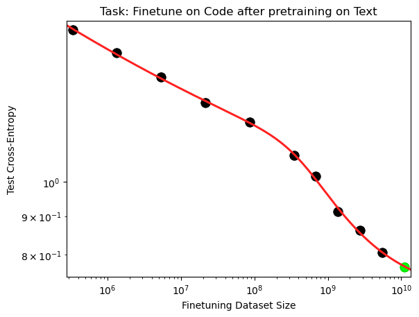
Figure 18: Extrapolation Results of BNSL with Finetuning Dataset Size on the X-axis. Experimental data is obtained from Figure 1 of Hernandez et al. (2021). The figure is of a transformer model that is pretrained on a large amount of mostly English text from the internet and then finetuned on a large amount of python code. The y-axis is Test Cross-Entropy on the distribution of python code. The x-axis is the size (measured in number of characters) of the Finetuning (not pretraining) Dataset. See Section A.20 for more details.

In Figure 18, we find BNSL accurately models and extrapolates the scaling behavior with finetuning dataset size on the x-axis (i.e. model that is pretrained on a large amount of mostly english text from the internet and then finetuned on a large amount of python code).

A.21 Extrapolation Results for Uncertainty Estimation / Calibration

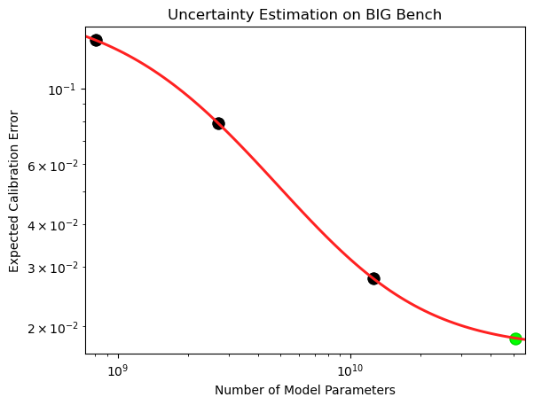
Figure 19: Extrapolation Results of BNSL for Uncertainty Estimation / Calibration. Expected Calibration Error is on the y-axis. Number of Model Parameters is on the x-axis. Experimental data obtained from “Lettered Choices (5-shot)” evaluation protocol plot from Figure 4 right of Kadavath et al. (2022). See Section A.21 for more details.

In Figure 19, we find BNSL accurately extrapolates the scaling behavior of downstream uncertainty estimation / calibration on BIG-Bench (Srivastava et al., 2022).

A.22 Extrapolation Results for AI Alignment via RLHF

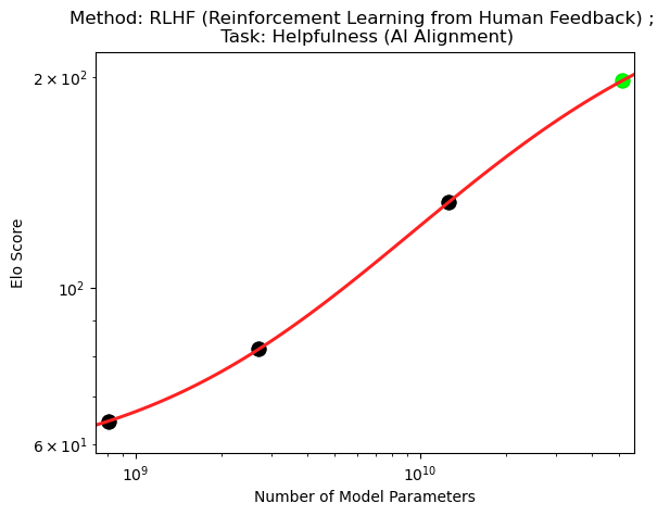
Figure 20: Extrapolation Results of BNSL for Downstream AI Alignment when Number of Model Parameters is on the x-axis. Experimental data obtained from the Static HH RLHF results from Figure 1 of Bai et al. (2022). See Section A.22 for more details.

In Figure 20, we find BNSL accurately extrapolates the scaling behavior of a pretrained language model finetuned (i.e. aligned) via Reinforcement Learning from Human Feedback (RLHF) to be helpful from Figure 1 of Bai et al. (2022). The y-axis is Elo score based on crowdworker preferences. The x-axis is the number of model parameters that the language model contains.

A.23 Extrapolation Results for Continual Learning (i.e. Catastrophic Forgetting)

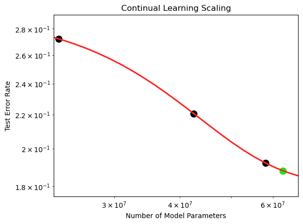
Figure 21: Extrapolation Results of BNSL for Continual Learning (i.e. Catastrophic Forgetting). Experimental data obtained from the Domainnet/Clipart section of the bottom right of Figure 2 of Ramasesh et al. (2022). X-axis is number of model parameters in the ResNet model. In this setup, model is trained (in sequence, not simultaneously) on task A and then task B. Y-axis is mean of the test error rate on task A and task B. See Section A.23 for more details.

In Figure 21, we find that BNSL accurately extrapolates the scaling behavior of continual learning (i.e. catastrophic forgetting).

A.24 Extrapolation Results for Robotics (Out-of-Distribution Generalization and In-distribution Generalization)

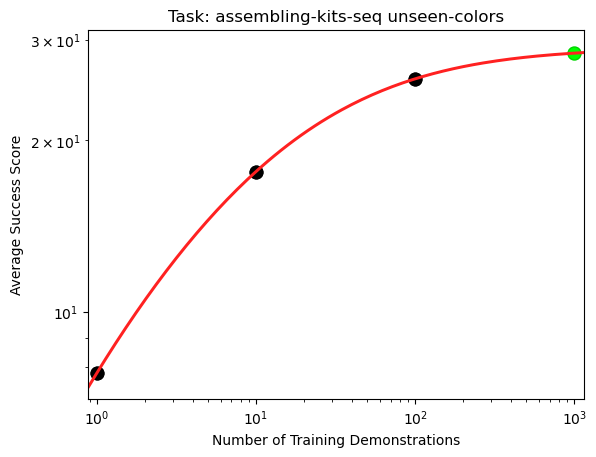
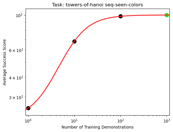
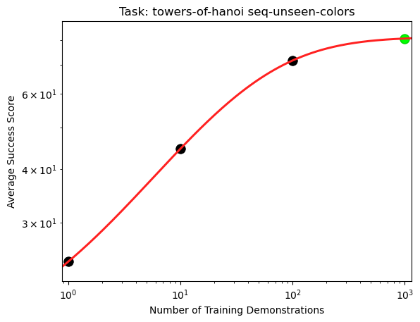
Figure 22: Extrapolation Results of BNSL for Robotic control (and Out-of-Distribution Generalization). Experimental data obtained from the transporter (Zeng et al., 2021) model results from Table 1 of Shridhar et al. (2021). X-axis is number of training demonstrations. Y-axis is task success score (mean percentage) obtained via 100 evaluations. See Section A.24 for more details.

In Figure 22, we find BNSL accurately extrapolates the scaling behavior of a transporter (Zeng et al., 2021) model trained via imitation learning to do robotic control tasks. Plots with “unseen-colors” in the plot title evaluate on a test set that contains colors that are unseen (i.e. out-of-distribution) with respect to the training set. Plots with “seen-colors” in the plot title evaluate on a test set that contains colors that are seen (i.e. in-distribution) with respect to the training set.

A.25 Extrapolation Results for Quantization

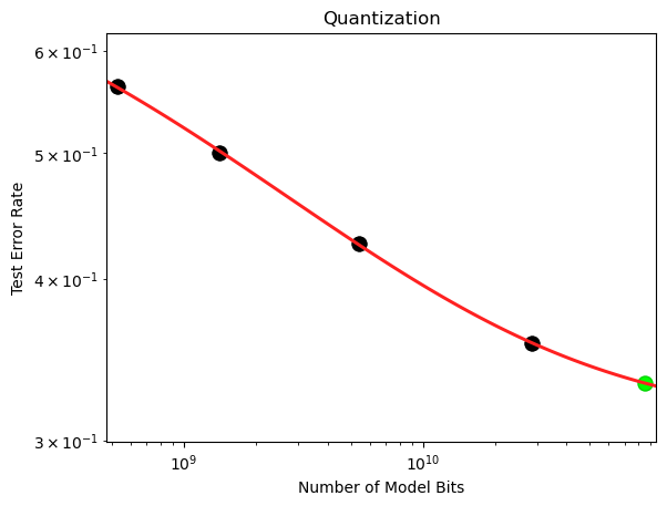
Figure 23: Extrapolation Results of BNSL for Quantization. Experimental data obtained from the 4 Bit Pythia (blockwise 64) results from Figure 8 bottom of Dettmers & Zettlemoyer (2022) in which an originally 16 bits (per parameter) model has been quantized to be 4 bits (per parameter) model. Y-axis is mean downstream zero-shot test error rate across Lambada, PiQA, Winogrande, and Hellaswag. X-axis is number of bits of parameters of model. See Section A.25 for more details.

In Figure 23, we find BNSL accurately extrapolates the scaling behavior (even downstream) of quantized models.

A.26 Extrapolation Results for Distillation

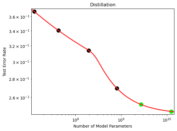
Figure 24: Extrapolation Results of BNSL for Distillation. Experimental data obtained from the Context Distillation results from Figure 5 left of Bai et al. (2022). In this setup, a language model (with the number of model parameters on the x-axis of this figure) that has been prompted is distilled into a language model (with the number of model parameters on the x-axis of this figure). Y-axis is test error rate on the helpful honest harmless (HHH) evaluation of Askell et al. (2021). See Section A.26 for more details.

In Figure 24, we find BNSL accurately extrapolates the scaling behavior of distillation (even to scales over an order of magnitude larger than the maximum (along the x-axis) of the points used for fitting).

A.27 Extrapolation Results for Out-of-Distribution Detection

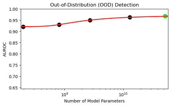
Figure 25: Extrapolation Results of BNSL for Out-of-Distribution Detection. Number of model parameters is on the x-axis. Y-axis is AUROC. Experimental data obtained from the Outlier Exposure results from Figure 23 of Bai et al. (2022) when exposed to 30 outlier examples. See Section A.27 for more details.

In Figure 25, we find BNSL accurately extrapolates the scaling behavior of Out-of-Distribution Detection performance (even to scales over an order of magnitude larger than the maximum (along the x-axis) of the points used for fitting).

A.28 Extrapolation Results for Molecules

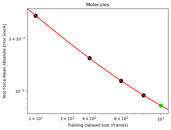
Figure 26: Extrapolation Results of BNSL for Molecules. Experimental data obtained from the “NequIP L=3” results for the aspirin molecule in MD-17 of Figure 8 of the arXiv version of Batzner et al. (2022). Y-axis is the test force mean absolute error [eV/A]. X-axis is the training dataset size (frames). See Section A.28 for more details.

In Figure 26, we find BNSL accurately extrapolates the scaling behavior of Neural Equivariant Interatomic Potentials (NequIP) graph neural networks (Batzner et al., 2022) trained via minimizing the weighted sum of energy and a force loss terms in order to predict the forces of molecules.

A.29 Extrapolation Results for Math Word Problems

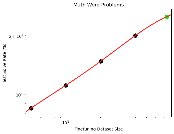
Figure 27: Extrapolation Results of BNSL for Math Word Problems. Experimental data obtained from the 12 billion parameter model results in Figure 2 left of Cobbe et al. (2021a). Y-axis is the test solve rate. X-axis is the finetuning dataset size. See Section A.29 for more details.

In Figure 27, we find BNSL accurately extrapolates the scaling behavior of large language models finetuned to solve math word problems.

A.30 Extrapolation Results for Fairness (and also Ensembles)

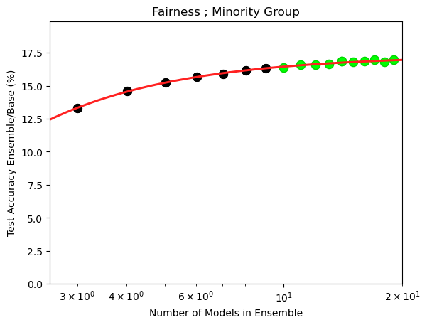
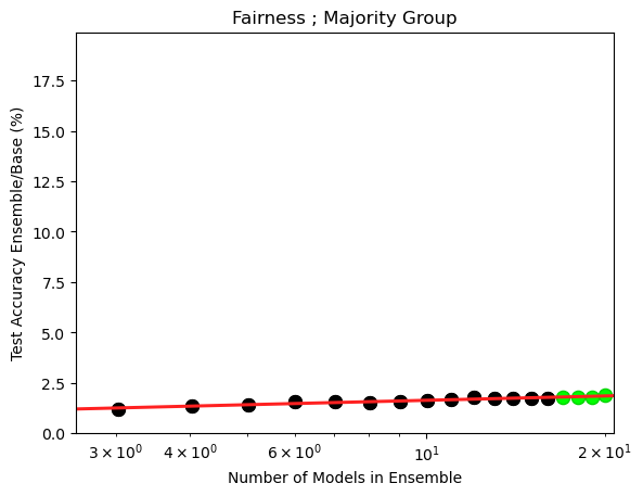
Figure 28: Extrapolation Results of BNSL for Fairness. Experimental data obtained from the Resnet-34 CIFAR-100 results in Figure 1 left of Ko et al. (2023). The model in this setup is an ensemble model. X-axis the number of models in the ensemble. Y-axis is the ratio of the ensemble’s accuracy over that of a single base model. In left plot, the test dataset is the minority group which is the bottom-10 classes that are least accurately predicted. In right plot, the test dataset is the majority group which is the top-10 classes that are most accurately predicted. See Section A.30 for more details.

In Figure 28, we find BNSL accurately extrapolates the scaling behavior of fairness (and also ensembles).

A.31 Extrapolation Results with Amount of Test-Time (a.k.a. Inference) Compute on the X-axis

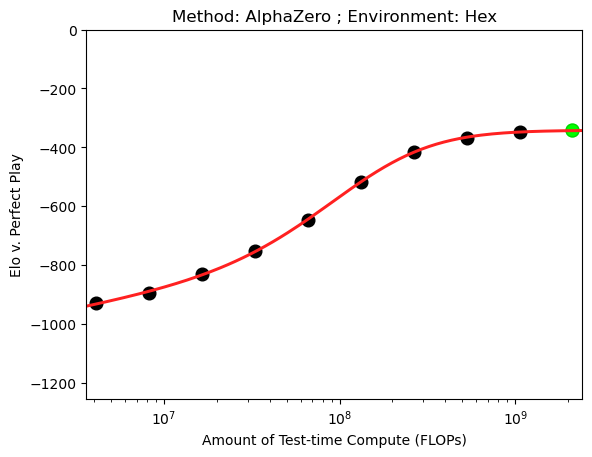
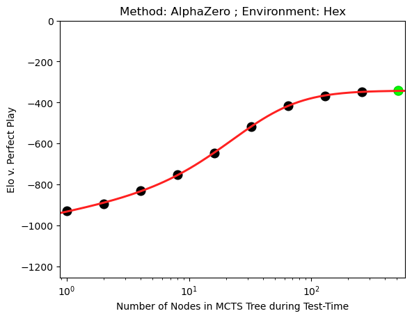
Figure 29: Extrapolation Results of BNSL with Test-Time Compute on the X-axis. Experimental data obtained from the “2x128” results in Figure 8 of Jones (2021). Y-axis is Elo score v. Perfect Play. The test-time scaling behavior in the plots is that of AlphaZero that has been trained to play Hex. In the right plot, x-axis is the number of nodes in the Monte Carlo tree search (MCTS) during test-time; note that the number of nodes in MCTS is held constant (at node count 64) during training for all variations of the x-axis, so the variations in the y-axis are 100% due to variations in the number of nodes in the MCTS during test-time (not training-time). Left plot is the same as the right plot but with the x-axis replaced with the amount of Test-Time Compute used to perform MCTS (with that number of nodes) during test-time. As a result, the x-axis of left plot is simply the x-axis of right plot multiplied times $\sim$$4120000$ which corresponds to the FLOPs per node of MCTS. See Section A.31 for more details.

In Figure 29, we find BNSL accurately extrapolates the scaling behavior when the amount of test-time (a.k.a. inference) compute (available to the model) is on the x-axis.

A.32 Extrapolation Results for Recurrent Neural Networks

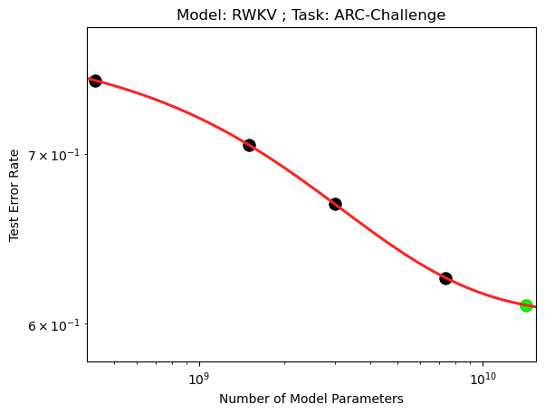
Figure 30: Extrapolation Results of BNSL for Recurrent Neural Networks. Experimental data obtained from the RWKV-4 ARC-c results in Table 3 of Peng et al. (2023). Y-axis is the downstream zero-shot test error rate on the ARC Challenge dataset. X-axis is the number of model parameters. See Section A.32 for more details.

In Figure 30, we find BNSL accurately extrapolates the scaling behavior of recurrent neural networks (even downstream).

A.33 Extrapolation Results for Downstream Performance of Multimodal Contrastive Learning (e.g. Non-Generative Unsupervised Learning)

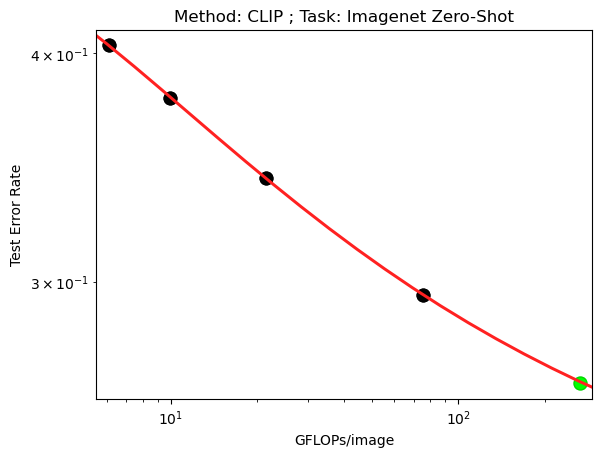
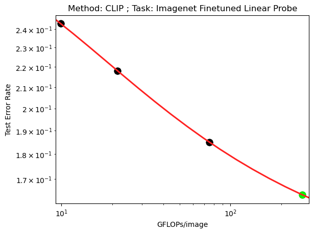
Figure 31: Extrapolation Results of BNSL for Downstream Performance of Multimodal Contrastive Learning (e.g. Non-Generative Unsupervised Learning). Experimental data of scaling behavior obtained from Table 10 and Table 11 in arXiv version of Radford et al. (2021). The upstream task is “Contrastive Image Language Pretraining” (a.k.a. CLIP) of ResNets on a training dataset consisting of hundreds of millions of image-text pairs. The x-axis is GFLOPs/image (GigaFLOPs/image) of the forward-pass of model. The Downstream Task is ImageNet classification (i.e. the y-axis of plot). The y-axis of left plot is Zero-Shot Downstream. The y-axis of right plot is performance of model with finetuned linear probe on it. See Section A.33 for more details.

In Figure 31, we show that BNSL accurately extrapolates the scaling behavior of the Downstream Performance of Multimodal Contrastive Learning (e.g. Non-Generative Unsupervised Learning).

A.34 Extrapolation Results for Downstream Performance on Audio Tasks

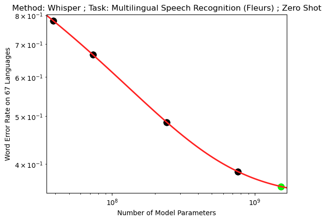
Figure 32: Extrapolation Results of BNSL for Downstream Audio Tasks when Number of Model Parameters is on the x-axis. Experimental data obtained from the second plot of Figure 6 of Whisper paper (Radford et al., 2022). The downstream task in the plot is downstream zero shot multilingual speech recognition performance on the FLEURS dataset of “Whisper” speech recognition model pretrained on a dataset of 681,070 hours of audio. See Section A.34 for more details.

In Figure 32, we show that BNSL accurately extrapolates the scaling behavior of the Downstream Performance on Audio Tasks.

A.35 Extrapolation Results for Downstream Performance (e.g. on Language/Coding Tasks) to scales that are greater than 100,000 times larger than the maximum (along the x-axis (e.g. amount of compute used for training)) of the points used for fitting

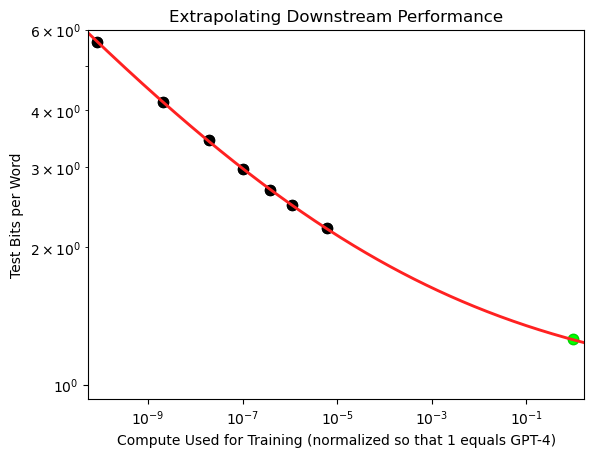
Figure 33: Extrapolation Results of BNSL for Downstream Performance (e.g. on Language/Coding Tasks) to scales that are greater than 100,000 (i.e. greater than 5 orders of magnitude) times larger than the maximum (along the x-axis (e.g. amount of compute used for training)) of the points used for fitting. Experimental data obtained from Figure 1 of GPT-4 paper (OpenAI, 2023). Each point corresponds to a different individual training run. The downstream evaluation (i.e. the y-axis) in the plot is downstream zero-shot test bits per word on OpenAI’s internal codebase (which was held out from the training set). The x-axis is normalized (i.e. divided by the amount of compute used to train GPT-4) such that 1 (i.e. where the green point is) is the amount of compute used to train GPT-4. Given that other language models released before GPT-4 used greater than 1e24 FLOPs of training compute and that GPT-4 is considerably more capable than those other language models, one can speculatively estimate that amount of compute used to train GPT-4 is probably an amount that is greater than 1e24 FLOPs. See Section A.35 for more details.

In Figure 33, we show that BNSL accurately extrapolates the scaling behavior of Downstream Performance (e.g. on Language/Coding Tasks) to scales that are greater than 100,000 (i.e. greater than 5 orders of magnitude) times larger than the maximum (along the x-axis (e.g. amount of compute used for training)) of the points used for fitting.

A.36 Plots of BNSL Extrapolations on Scaling Laws Benchmark of Alabdulmohsin et al. (2022)

References

- dam (2017) Direct detection of a break in the teraelectronvolt cosmic-ray spectrum of electrons and positrons. Nature, 552(7683):63–66, nov 2017. doi: 10.1038/nature24475. URL https://doi.org/10.1038%2Fnature24475.
- Abnar et al. (2021) Samira Abnar, Mostafa Dehghani, Behnam Neyshabur, and Hanie Sedghi. Exploring the limits of large scale pre-training, 2021.
- Ainslie et al. (2023) Joshua Ainslie, Tao Lei, Michiel de Jong, Santiago Ontañón, Siddhartha Brahma, Yury Zemlyanskiy, David Uthus, Mandy Guo, James Lee-Thorp, Yi Tay, Yun-Hsuan Sung, and Sumit Sanghai. Colt5: Faster long-range transformers with conditional computation, 2023.
- Alabdulmohsin et al. (2022) Ibrahim Mansour I Alabdulmohsin, Behnam Neyshabur, and Xiaohua Zhai. Revisiting neural scaling laws in language and vision. In NeurIPS 2022, 2022. URL https://arxiv.org/abs/2209.06640.
- Askell et al. (2021) Amanda Askell, Yuntao Bai, Anna Chen, Dawn Drain, Deep Ganguli, Tom Henighan, Andy Jones, Nicholas Joseph, Ben Mann, Nova DasSarma, et al. A general language assistant as a laboratory for alignment. arXiv preprint arXiv:2112.00861, 2021.
- Bahri et al. (2021) Yasaman Bahri, Ethan Dyer, Jared Kaplan, Jaehoon Lee, and Utkarsh Sharma. Explaining neural scaling laws. arXiv preprint arXiv:2102.06701, 2021.
- Bai et al. (2022) Yuntao Bai, Andy Jones, Kamal Ndousse, Amanda Askell, Anna Chen, Nova DasSarma, Dawn Drain, Stanislav Fort, Deep Ganguli, Tom Henighan, et al. Training a helpful and harmless assistant with reinforcement learning from human feedback. arXiv preprint arXiv:2204.05862, 2022.
- Bansal et al. (2022) Yamini Bansal, Behrooz Ghorbani, Ankush Garg, Biao Zhang, Colin Cherry, Behnam Neyshabur, and Orhan Firat. Data scaling laws in nmt: The effect of noise and architecture. In International Conference on Machine Learning, pp. 1466–1482. PMLR, 2022.
- Batzner et al. (2022) Simon Batzner, Albert Musaelian, Lixin Sun, Mario Geiger, Jonathan P. Mailoa, Mordechai Kornbluth, Nicola Molinari, Tess E. Smidt, and Boris Kozinsky. E(3)-equivariant graph neural networks for data-efficient and accurate interatomic potentials. Nature Communications, 13(1), may 2022. doi: 10.1038/s41467-022-29939-5. URL https://doi.org/10.1038%2Fs41467-022-29939-5.
- Borgeaud et al. (2022) Sebastian Borgeaud, Arthur Mensch, Jordan Hoffmann, Trevor Cai, Eliza Rutherford, Katie Millican, George Bm Van Den Driessche, Jean-Baptiste Lespiau, Bogdan Damoc, Aidan Clark, et al. Improving language models by retrieving from trillions of tokens. In International conference on machine learning, pp. 2206–2240. PMLR, 2022.
- Brown et al. (2020) Tom Brown, Benjamin Mann, Nick Ryder, Melanie Subbiah, Jared D Kaplan, Prafulla Dhariwal, Arvind Neelakantan, Pranav Shyam, Girish Sastry, Amanda Askell, et al. Language models are few-shot learners. Advances in neural information processing systems, 33:1877–1901, 2020.
- Clark et al. (2022) Aidan Clark, Diego De Las Casas, Aurelia Guy, Arthur Mensch, Michela Paganini, Jordan Hoffmann, Bogdan Damoc, Blake Hechtman, Trevor Cai, Sebastian Borgeaud, et al. Unified scaling laws for routed language models. In International Conference on Machine Learning, pp. 4057–4086. PMLR, 2022.
- Cobbe et al. (2020) Karl Cobbe, Chris Hesse, Jacob Hilton, and John Schulman. Leveraging procedural generation to benchmark reinforcement learning. In International conference on machine learning, pp. 2048–2056. PMLR, 2020.
- Cobbe et al. (2021a) Karl Cobbe, Vineet Kosaraju, Mohammad Bavarian, Mark Chen, Heewoo Jun, Lukasz Kaiser, Matthias Plappert, Jerry Tworek, Jacob Hilton, Reiichiro Nakano, et al. Training verifiers to solve math word problems. arXiv preprint arXiv:2110.14168, 2021a.
- Cobbe et al. (2021b) Karl W Cobbe, Jacob Hilton, Oleg Klimov, and John Schulman. Phasic policy gradient. In International Conference on Machine Learning, pp. 2020–2027. PMLR, 2021b.
- Cortes et al. (1994) Corinna Cortes, Lawrence D Jackel, Sara A Solla, Vladimir Vapnik, and John S Denker. Learning curves: Asymptotic values and rate of convergence. In Advances in Neural Information Processing Systems, pp. 327–334, 1994.
- Deng et al. (2009) Jia Deng, Wei Dong, Richard Socher, Li-Jia Li, Kai Li, and Li Fei-Fei. Imagenet: A large-scale hierarchical image database. In 2009 IEEE conference on computer vision and pattern recognition, pp. 248–255. Ieee, 2009.
- Dettmers & Zettlemoyer (2022) Tim Dettmers and Luke Zettlemoyer. The case for 4-bit precision: k-bit inference scaling laws. arXiv preprint arXiv:2212.09720, 2022.
- Dosovitskiy et al. (2020) Alexey Dosovitskiy, Lucas Beyer, Alexander Kolesnikov, Dirk Weissenborn, Xiaohua Zhai, Thomas Unterthiner, Mostafa Dehghani, Matthias Minderer, Georg Heigold, Sylvain Gelly, et al. An image is worth 16x16 words: Transformers for image recognition at scale. arXiv preprint arXiv:2010.11929, 2020.
- Evans et al. (2021) Owain Evans, Owen Cotton-Barratt, Lukas Finnveden, Adam Bales, Avital Balwit, Peter Wills, Luca Righetti, and William Saunders. Truthful ai: Developing and governing ai that does not lie. arXiv preprint arXiv:2110.06674, 2021.
- Fei-Fei et al. (2004) Li Fei-Fei, Rob Fergus, and Pietro Perona. Learning generative visual models from few training examples: An incremental bayesian approach tested on 101 object categories. In 2004 conference on computer vision and pattern recognition workshop, pp. 178–178. IEEE, 2004.
- Frantar & Alistarh (2023) Elias Frantar and Dan Alistarh. Massive language models can be accurately pruned in one-shot. arXiv preprint arXiv:2301.00774, 2023.
- Ganguli et al. (2022) Deep Ganguli, Danny Hernandez, Liane Lovitt, Amanda Askell, Yuntao Bai, Anna Chen, Tom Conerly, Nova Dassarma, Dawn Drain, Nelson Elhage, et al. Predictability and surprise in large generative models. In 2022 ACM Conference on Fairness, Accountability, and Transparency, pp. 1747–1764, 2022.
- Hendrycks & Mazeika (2022) Dan Hendrycks and Mantas Mazeika. X-risk analysis for ai research. arXiv preprint arXiv:2206.05862, 2022.
- Henighan et al. (2020) Tom Henighan, Jared Kaplan, Mor Katz, Mark Chen, Christopher Hesse, Jacob Jackson, Heewoo Jun, Tom B. Brown, Prafulla Dhariwal, Scott Gray, Chris Hallacy, Benjamin Mann, Alec Radford, Aditya Ramesh, Nick Ryder, Daniel M. Ziegler, John Schulman, Dario Amodei, and Sam McCandlish. Scaling Laws for Autoregressive Generative Modeling. arXiv e-prints, art. arXiv:2010.14701, October 2020.
- Hernandez et al. (2021) Danny Hernandez, Jared Kaplan, Tom Henighan, and Sam McCandlish. Scaling Laws for Transfer. arXiv e-prints, art. arXiv:2102.01293, February 2021.
- Hestness et al. (2017) Joel Hestness, Sharan Narang, Newsha Ardalani, Gregory Diamos, Heewoo Jun, Hassan Kianinejad, Md. Mostofa Ali Patwary, Yang Yang, and Yanqi Zhou. Deep Learning Scaling is Predictable, Empirically. arXiv e-prints, art. arXiv:1712.00409, December 2017.
- Hilton et al. (2023) Jacob Hilton, Jie Tang, and John Schulman. Scaling laws for single-agent reinforcement learning. arXiv preprint arXiv:2301.13442, 2023.
- Hunter (2007) J. D. Hunter. Matplotlib: A 2d graphics environment. Computing in Science & Engineering, 9(3):90–95, 2007. doi: 10.1109/MCSE.2007.55.
- Jones (2021) Andy L Jones. Scaling scaling laws with board games. arXiv preprint arXiv:2104.03113, 2021.
- Kadavath et al. (2022) Saurav Kadavath, Tom Conerly, Amanda Askell, Tom Henighan, Dawn Drain, Ethan Perez, Nicholas Schiefer, Zac Hatfield Dodds, Nova DasSarma, Eli Tran-Johnson, et al. Language models (mostly) know what they know. arXiv preprint arXiv:2207.05221, 2022.
- Kaplan et al. (2020) Jared Kaplan, Sam McCandlish, Tom Henighan, Tom B. Brown, Benjamin Chess, Rewon Child, Scott Gray, Alec Radford, Jeffrey Wu, and Dario Amodei. Scaling Laws for Neural Language Models. arXiv e-prints, art. arXiv:2001.08361, January 2020.
- Karpathy (2020) Andrej Karpathy. mingpt. https://github.com/karpathy/minGPT, 2020.
- Ko et al. (2023) Wei-Yin Ko, Daniel D’souza, Karina Nguyen, Randall Balestriero, and Sara Hooker. Fair-ensemble: When fairness naturally emerges from deep ensembling. arXiv preprint arXiv:2303.00586, 2023.
- Kočiskỳ et al. (2018) Tomáš Kočiskỳ, Jonathan Schwarz, Phil Blunsom, Chris Dyer, Karl Moritz Hermann, Gábor Melis, and Edward Grefenstette. The narrativeqa reading comprehension challenge. Transactions of the Association for Computational Linguistics, 6:317–328, 2018.
- Kolesnikov et al. (2020) Alexander Kolesnikov, Lucas Beyer, Xiaohua Zhai, Joan Puigcerver, Jessica Yung, Sylvain Gelly, and Neil Houlsby. Big transfer (bit): General visual representation learning. In European conference on computer vision, pp. 491–507. Springer, 2020.
- Krizhevsky et al. (2009) Alex Krizhevsky, Geoffrey Hinton, et al. Learning multiple layers of features from tiny images. 2009.
- Lin et al. (2021) Stephanie Lin, Jacob Hilton, and Owain Evans. Truthfulqa: Measuring how models mimic human falsehoods. arXiv preprint arXiv:2109.07958, 2021.
- Madry et al. (2018) Aleksander Madry, Aleksandar Makelov, Ludwig Schmidt, Dimitris Tsipras, and Adrian Vladu. Towards deep learning models resistant to adversarial attacks. In International Conference on Learning Representations, 2018. URL https://openreview.net/forum?id=rJzIBfZAb.
- Nakkiran et al. (2021) Preetum Nakkiran, Gal Kaplun, Yamini Bansal, Tristan Yang, Boaz Barak, and Ilya Sutskever. Deep double descent: Where bigger models and more data hurt. Journal of Statistical Mechanics: Theory and Experiment, 2021(12):124003, 2021.
- Neumann & Gros (2022) Oren Neumann and Claudius Gros. Scaling laws for a multi-agent reinforcement learning model. arXiv preprint arXiv:2210.00849, 2022.
- Nichol & Dhariwal (2021) Alexander Quinn Nichol and Prafulla Dhariwal. Improved denoising diffusion probabilistic models. In International Conference on Machine Learning, pp. 8162–8171. PMLR, 2021.
- OpenAI (2023) OpenAI. Gpt-4 technical report. ArXiv, abs/2303.08774, 2023.
- Peng et al. (2023) Bo Peng, Eric Alcaide, Quentin Anthony, Alon Albalak, Samuel Arcadinho, Huanqi Cao, Xin Cheng, Michael Chung, Matteo Grella, Kranthi Kiran GV, et al. Rwkv: Reinventing rnns for the transformer era. arXiv preprint arXiv:2305.13048, 2023.
- Power et al. (2022) Alethea Power, Yuri Burda, Harri Edwards, Igor Babuschkin, and Vedant Misra. Grokking: Generalization beyond overfitting on small algorithmic datasets. arXiv preprint arXiv:2201.02177, 2022.
- Radford et al. (2021) Alec Radford, Jong Wook Kim, Chris Hallacy, Aditya Ramesh, Gabriel Goh, Sandhini Agarwal, Girish Sastry, Amanda Askell, Pamela Mishkin, Jack Clark, et al. Learning transferable visual models from natural language supervision. In International Conference on Machine Learning, pp. 8748–8763. PMLR, 2021.
- Radford et al. (2022) Alec Radford, Jong Wook Kim, Tao Xu, Greg Brockman, Christine McLeavey, and Ilya Sutskever. Robust speech recognition via large-scale weak supervision. arXiv preprint arXiv:2212.04356, 2022.
- Raffel et al. (2019) Colin Raffel, Noam Shazeer, Adam Roberts, Katherine Lee, Sharan Narang, Michael Matena, Yanqi Zhou, Wei Li, and Peter J. Liu. Exploring the limits of transfer learning with a unified text-to-text transformer. arXiv e-prints, 2019.
- Ramasesh et al. (2022) Vinay Venkatesh Ramasesh, Aitor Lewkowycz, and Ethan Dyer. Effect of scale on catastrophic forgetting in neural networks. In International Conference on Learning Representations, 2022.
- Rosenfeld et al. (2019) Jonathan S. Rosenfeld, Amir Rosenfeld, Yonatan Belinkov, and Nir Shavit. A constructive prediction of the generalization error across scales. CoRR, abs/1909.12673, 2019. URL http://arxiv.org/abs/1909.12673.
- Rosenfeld et al. (2021) Jonathan S Rosenfeld, Jonathan Frankle, Michael Carbin, and Nir Shavit. On the predictability of pruning across scales. arXiv preprint arXiv:2006.10621, 2021.
- Schulman et al. (2017) John Schulman, Filip Wolski, Prafulla Dhariwal, Alec Radford, and Oleg Klimov. Proximal policy optimization algorithms. arXiv preprint arXiv:1707.06347, 2017.
- Shridhar et al. (2021) Mohit Shridhar, Lucas Manuelli, and Dieter Fox. Cliport: What and where pathways for robotic manipulation. In Proceedings of the 5th Conference on Robot Learning (CoRL), 2021.
- Silver et al. (2017) David Silver, Thomas Hubert, Julian Schrittwieser, Ioannis Antonoglou, Matthew Lai, Arthur Guez, Marc Lanctot, Laurent Sifre, Dharshan Kumaran, Thore Graepel, et al. Mastering chess and shogi by self-play with a general reinforcement learning algorithm. arXiv preprint arXiv:1712.01815, 2017.
- Sorscher et al. (2022) Ben Sorscher, Robert Geirhos, Shashank Shekhar, Surya Ganguli, and Ari S. Morcos. Beyond neural scaling laws: beating power law scaling via data pruning, 2022. URL https://arxiv.org/abs/2206.14486.
- Srivastava et al. (2022) Aarohi Srivastava, Abhinav Rastogi, Abhishek Rao, Abu Awal Md Shoeb, Abubakar Abid, Adam Fisch, Adam R Brown, Adam Santoro, Aditya Gupta, Adrià Garriga-Alonso, et al. Beyond the imitation game: Quantifying and extrapolating the capabilities of language models. arXiv preprint arXiv:2206.04615, 2022.
- Sun et al. (2017) Chen Sun, Abhinav Shrivastava, Saurabh Singh, and Abhinav Gupta. Revisiting unreasonable effectiveness of data in deep learning era. In Proceedings of the IEEE international conference on computer vision, pp. 843–852, 2017.
- Tolstikhin et al. (2021) Ilya O Tolstikhin, Neil Houlsby, Alexander Kolesnikov, Lucas Beyer, Xiaohua Zhai, Thomas Unterthiner, Jessica Yung, Andreas Steiner, Daniel Keysers, Jakob Uszkoreit, et al. Mlp-mixer: An all-mlp architecture for vision. Advances in Neural Information Processing Systems, 34:24261–24272, 2021.
- Van Den Oord et al. (2017) Aaron Van Den Oord, Oriol Vinyals, et al. Neural discrete representation learning. Advances in neural information processing systems, 30, 2017.
- Vaswani et al. (2017) Ashish Vaswani, Noam Shazeer, Niki Parmar, Jakob Uszkoreit, Llion Jones, Aidan N Gomez, Łukasz Kaiser, and Illia Polosukhin. Attention is all you need. Advances in neural information processing systems, 30, 2017.
- Virtanen et al. (2020) Pauli Virtanen, Ralf Gommers, Travis E Oliphant, Matt Haberland, Tyler Reddy, David Cournapeau, Evgeni Burovski, Pearu Peterson, Warren Weckesser, Jonathan Bright, et al. Scipy 1.0: fundamental algorithms for scientific computing in python. Nature methods, 17(3):261–272, 2020.
- Wei et al. (2022a) Jason Wei, Yi Tay, Rishi Bommasani, Colin Raffel, Barret Zoph, Sebastian Borgeaud, Dani Yogatama, Maarten Bosma, Denny Zhou, Donald Metzler, et al. Emergent abilities of large language models. arXiv preprint arXiv:2206.07682, 2022a.
- Wei et al. (2022b) Jason Wei, Xuezhi Wang, Dale Schuurmans, Maarten Bosma, Ed Chi, Quoc Le, and Denny Zhou. Chain of thought prompting elicits reasoning in large language models. arXiv preprint arXiv:2201.11903, 2022b.
- Welinder et al. (2010) Peter Welinder, Steve Branson, Takeshi Mita, Catherine Wah, Florian Schroff, Serge Belongie, and Pietro Perona. Caltech-ucsd birds 200. 2010.
- Xie & Yuille (2020) Cihang Xie and Alan Yuille. Intriguing properties of adversarial training at scale. In International Conference on Learning Representations, 2020. URL https://openreview.net/forum?id=HyxJhCEFDS.
- Zeng et al. (2021) Andy Zeng, Pete Florence, Jonathan Tompson, Stefan Welker, Jonathan Chien, Maria Attarian, Travis Armstrong, Ivan Krasin, Dan Duong, Vikas Sindhwani, et al. Transporter networks: Rearranging the visual world for robotic manipulation. In Conference on Robot Learning, pp. 726–747. PMLR, 2021.
- Zhai et al. (2021) Xiaohua Zhai, Alexander Kolesnikov, Neil Houlsby, and Lucas Beyer. Scaling vision transformers. CoRR, abs/2106.04560, 2021. URL https://arxiv.org/abs/2106.04560.