Quantum deep recurrent reinforcement learning

Abstract

Recent advances in quantum computing (QC) and machine learning (ML) have drawn significant attention to the development of quantum machine learning (QML). Reinforcement learning (RL) is one of the ML paradigms which can be used to solve complex sequential decision making problems. Classical RL has been shown to be capable to solve various challenging tasks. However, RL algorithms in the quantum world are still in their infancy. One of the challenges yet to solve is how to train quantum RL in the partially observable environments. In this paper, we approach this challenge through building QRL agents with quantum recurrent neural networks (QRNN). Specifically, we choose the quantum long short-term memory (QLSTM) to be the core of the QRL agent and train the whole model with deep $Q$-learning. We demonstrate the results via numerical simulations that the QLSTM-DRQN can solve standard benchmark such as Cart-Pole with more stable and higher average scores than classical DRQN with similar architecture and number of model parameters.

Index Terms—  Quantum machine learning, Reinforcement learning, Recurrent neural networks, Long short-term memory

1 Introduction

Quantum computing (QC) promises superior performance on certain hard computational tasks over classical computers [1]. However, existing quantum computers are not error-corrected, making implementation of deep quantum circuits extremely difficult. These so-called noisy intermediate-scale quantum (NISQ) devices [2] require special design of quantum circuit architectures so that the quantum advantages can be harnessed. Recently, a hybrid quantum-classical computing framework [3] which leverage both the classical and quantum computing has been proposed. Under this paradigm, certain computational tasks which are expected to have quantum advantages are carried out on a quantum computer, while other tasks such as gradient calculations remain on the classical computers. These algorithms are usually called variational quantum algorithms are have been successful in certain ML tasks. Reinforcement learning (RL) is a sub-field of ML dealing with sequential decision making tasks. RL based on deep neural networks have gained tremendous success in complex tasks with human-level [4] or super-human performance [5]. However, quantum RL is an emerging subject with many issues and challenges not yet investigated. For example, existing quantum RL methods focus on various VQCs without the recurrent structures. Nevertheless, recurrent connections are crucial components in the classical ML to keep memory of past time steps. The potential of such architectures, to our best knowledge, is not yet studied in the quantum RL. In this work, we propose the quantum deep recurrent $Q$-learning via the application of quantum recurrent neural networks (QRNN) as the value function approximator. Specifically, we apply the quantum long short-term memory (QLSTM) as the core of the QRL agent. The scheme is illustrated in Figure 1. Our numerical simulation shows that the proposed framework can reach performance comparable to or better than their classical LSTM counterparts when the model sizes are similar and under the same training setting.

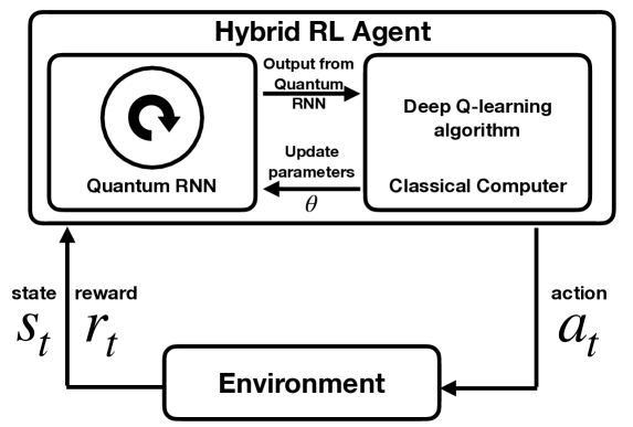
Fig. 1: The hybrid quantum-classical deep recurrent $Q$-learning.

2 Related Work

The quantum reinforcement learning (QRL) can be traced back to the work [6]. However, the framework requires the environment to be quantum, which may not be satisfied in most real-world cases. Here we focus on the recent developments of VQC-based QRL dealing with classical environments. The first VQC-based QRL [7], which is the quantum version of deep $Q$-learning (DQN), considers discrete observation and action spaces in the testing environments such as Frozen-Lake and Cognitive-Radio. Later, more advanced works in the direction of quantum deep $Q$-learning consider continuous observation spaces such as Cart-Pole [8, 9]. Hybrid quantum-classical linear solver are also used to find value functions. [10]. A further improvement of DQN to Double DQN (DDQN) in the VQC framework is considered in the work [11], which applies QRL to solve robot navigation task. In addition to learning the value functions such as the $Q$-function, QRL frameworks designed to learn the policy functions $\pi$ have been proposed recently. For example, the paper [12] describes the quantum policy gradient RL through the use of REINFORCE algorithm. Then, the work [13] consider an improved policy gradient algorithm called PPO with VQCs and show that quantum models with small amount of parameters can beat their classical counterparts. Along this direction, various modified quantum policy gradient algorithms are proposed such as actor-critic [14] and soft actor-critic (SAC) [15]. There are also applications of QRL in quantum control [16] and the proposal of QRL in the multi-agent setting [17]. QRL optimization with evolutionary optimization is first studied in [18]. Advanced quantum policy gradient such as DDPG which can deal with continuous action space is considered in [19]. In this work we consider the quantum deep recurrent $Q$-learning, which is an extension of the DQN discussed in [7, 8, 9]. However, our work is different from the aforementioned ones as our work consider the recurrent quantum policy, while previous works consider the application of various feed-forward VQC architectures. The recurrent policies considered in this work may provide benefits in environments requiring memory of previous steps.

3 Reinforcement Learning

Reinforcement learning (RL) is a machine learning framework in which an agent learns to achieve a given goal through interacting with an environment $\mathcal{E}$ over a sequence of discrete time steps [20]. At each time step $t$, the agent observes a state $s_{t}$ and then selects an action $a_{t}$ from the action space $\mathcal{A}$ according to its current policy $\pi$. The policy is a mapping from a certain state $s_{t}$ to the probabilities of selecting an action from $\mathcal{A}$. After exercising the action $a_{t}$, the agent receives a scalar reward $r_{t}$ and the state of the next time step $s_{t+1}$ from the environment. For episodic tasks, the process proceeds over a number of time steps until the agent reaches the terminal state or the maximum steps allowed. Seeing the state $s_{t}$ along the training process, the agent aims to maximize the expected return, which can be expressed as the value function at state $s$ under policy $\pi$, $V^{\pi}(s)=\mathbb{E}\left[R_{t}|s_{t}=s\right]$, where $R_{t}=\sum_{t^{\prime}=t}^{T}\gamma^{t^{\prime}-t}r_{t^{\prime}}$ is the return, the total discounted reward from time step $t$. The value function can be further expressed as $V^{\pi}(s)=\sum_{a\in\mathcal{A}}Q^{\pi}(s,a)\pi(a|s)$, where the action-value function or Q-value function $Q^{\pi}(s,a)=\mathbb{E}[R_{t}|s_{t}=s,a]$ is the expected return of choosing an action $a\in\mathcal{A}$ in state $s$ according to the policy $\pi$. The $Q$-learning is RL algorithm to optimize the $Q^{\pi}(s,a)$ via the following benchmark formula

$$Q\left(s_{t},a_{t}\right)\leftarrow \,Q\left(s_{t},a_{t}\right)$$

$$+\alpha\left[r_{t}+\gamma\max_{a}Q\left(s_{t+1},a\right)-Q\left(s_{t},a_{t}\right)\right].$$ (1)

The deep $Q$-learning [4] is an extension of the $Q$-learning via the inclusion of the experience replay and the target network to make the training of deep neural network-based $Q$-value function numerically stable. The deep recurrent $Q$-learning is when a recurrent neural network (RNN) is used to approximate the $Q$-value function [21].

4 Variational Quantum Circuits

Variational quantum circuits (VQC), also known as parameterized quantum circuits (PQC) in the literature, are a special kind of quantum circuits with trainable parameters. Those parameters are trained via optimization algorithms developed in the classical ML communities. The optimization can be gradient-based or gradient-free. The general form of a VQC is described in Figure 2

@C=1em @R=1em —0⟩ & 3U(x) 3V(θ)

—0⟩

U(x) V(θ)

—0⟩

U(x) V(θ)

—0⟩

U(x) V(θ)

Fig. 2: Generic architecture for variational quantum circuits (VQC).

There are three components in a VQC. The encoding block $U(\mathbf{x})$ is to transform the classical data $\mathbf{x}$ into a quantum state. The variational or parameterized block $V(\bm{\theta})$ represents the part with learnable parameters $\bm{\theta}$ that is optimized through gradient-descent method in this study. The final measurement is to output information through measuring a subset (or all) of the qubits and thereby retrieving a (classical) bit string. If we run the circuit once, we can get a bit string such as $0,0,1,1$. However, if we run the circuit multiple times, we can get the expectation values of each qubit. In this paper, we consider the Pauli-$Z$ expectation values of the VQC.

One of the benefits provided by the VQCs is that such circuits are more robust against quantum device noise [22, 23, 24]. This feature makes VQCs useful for the NISQ [2] era. In addition, it has been shown that VQCs mav be more expressive than classical neural networks [25, 26, 27, 28] and can be trained with smaller dataset [29]. Notable examples of VQC in QML include classification [30, 31, 32, 33, 34], natural language processing [35, 36, 37] and sequence modeling [38, 39].

5 METHODS

5.1 QLSTM

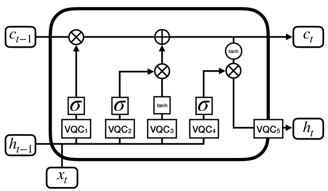
Fig. 3: The QLSTM used in the proposed quantum deep recurrent $Q$-learning.

The QLSTM (shown in Figure 3), first proposed in the work [38], is the quantum version of LSTM [40]. The main idea behind this model is that the classical neural networks are replaced by the VQCs. It has been shown to be capable of learning time-series data [38] and performing NLP tasks [37]. A formal mathematical formulation of a QLSTM cell is given by

$$f_{t} =\sigma\left(VQC_{1}(v_{t})\right)$$ (2a)

$$i_{t} =\sigma\left(VQC_{2}(v_{t})\right)$$ (2b)

$$\tilde{C}_{t} =\tanh\left(VQC_{3}(v_{t})\right)$$ (2c)

$$c_{t} =f_{t}*c_{t-1}+i_{t}*\tilde{C}_{t}$$ (2d)

$$o_{t} =\sigma\left(VQC_{4}(v_{t})\right)$$ (2e)

$$h_{t} =VQC_{5}(o_{t}*\tanh\left(c_{t}\right))$$ (2f)

where the input to the QLSTM is the concatenation $v_{t}$ of the hidden state $h_{t-1}$ from the previous time step and the current input vector $x_{t}$ which is the processed observation from the environment. The VQC component used in the QLSTM follows the design shown in Figure 4. This architecture has been shown to be highly successful in time-series modeling [38]. The data encoding part includes $R_{y}$ and $R_{z}$ rotations, the variational part includes multiple CNOT gates to entangle qubits and trainable general unitary $U$ gates. Finally, the quantum measurement follows.

@C=1em @R=1em —0⟩ & H R_y(arctan(x_1)) R_z(arctan(x_1^2)) 1 2 R(α_1, β_1, γ_1)

—0⟩

H R_y(arctan(x_2)) R_z(arctan(x_2^2)) 1 2 R(α_2, β_2, γ_2)

—0⟩

H R_y(arctan(x_3)) R_z(arctan(x_3^2)) 1 -2 R(α_3, β_3, γ_3)

—0⟩

H R_y(arctan(x_4)) R_z(arctan(x_4^2)) -3 -2 R(α_4, β_4, γ_4) 15413.7em–

Fig. 4: VQC architecture for QLSTM

5.2 Quantum Deep Recurrent Q-Learning

The proposed QDRQN includes the policy network $\theta$ and the target network $\theta^{-}$. Both of them are of the same architecture with a classical NN layer for preprocessing the input, a QLSTM core for the main decision making and a final classical NN layer for post-processing. Such kind of architecture is called dressed QLSTM model. During the training, the trajectories are stored in the replay memory so that in the optimization stage, these trajectories can be sampled and make the training more stable. The target network is updated every $S$ steps. The QDRQN algorithm is summarized in Algorithm. 1.

Initialize replay memory $\mathcal{D}$ to capacity $N$

Initialize action-value function dressed QLSTM $Q$ with random parameters $\theta$

Initialize target dressed QLSTM $Q$ with $\theta^{-}=\theta$

for episode $=1,2,\ldots,M$ do

     Initialize the episode record buffer $\mathcal{M}$

     Initialise state $s_{1}$ and encode into the quantum state

     Initialize $h_{1}$ and $c_{1}$ for the QLSTM

     for $t=1,2,\ldots,T$ do

         With probability $\epsilon$ select a random action $a_{t}$

         otherwise select $a_{t}=\max_{a}Q^{*}(s_{t},a;\theta)$ from the output of the QLSTM

         Execute action $a_{t}$ in emulator and observe reward $r_{t}$ and next state $s_{t+1}$

         Store transition $\left(s_{t},a_{t},r_{t},s_{t+1}\right)$ in $\mathcal{M}$

         Sample random batch of trajectories $\mathcal{T}$ from $\mathcal{D}$

         Set $y_{j}=\left\{\begin{array}[]{l}r_{j}\quad\text{for terminal }s_{j+1}\\ r_{j}+\gamma\max_{a^{\prime}}Q(s_{j+1},a^{\prime};\theta)\\ \quad\text{for non-terminal }s_{j+1}\end{array}\right.$

         Perform a gradient descent step on $\left(y_{j}-Q(s_{j},a_{j};\theta^{-})\right)^{2}$

         Update the target network $\theta^{-}$ every $S$ steps.

     end for

     Store episode record $\mathcal{M}$ to $\mathcal{D}$

     Update $\epsilon$

end for

Algorithm 1 Quantum deep recurrent $Q$-learning

6 Experiments

6.1 Environment

The testing environment we choose in this work is Cart-Pole, a standard control problem for benchmarking simple RL models and is also a commonly used example in the OpenAI Gym [41]. In this environment, a pole is attached by a fixed joint to a cart moving horizontally along a frictionless track. The goal of the RL agent is to learn to output the appropriate action according to the observation it receives at each time step so that it can keep the pole as close to the initial state (upright) as possible by pushing the cart leftwards and rightwards. The Cart-Pole environment mapping is: Observation: A four dimensional vector $s_{t}$ including values of the cart position, cart velocity, pole angle, and pole velocity at the tip; Action: There are two actions $+1$ (pushing rightwards) and $-1$ (pushing leftwards) in the action space; Reward: A reward of $+1$ is given for every time step where the pole remains close to being upright. An episode terminates if the pole is angled over $15$ degrees from vertical, or the cart moves away from the center more than $2.4$ units.

6.2 Hyperparameters

The hyperparameters for the proposed QDRQN are: batch size: 8, learning rate (Adam): $1\times 10^{-3}$, memory buffer length $N$: 100, lookup steps $L$: 10. The $\epsilon$-greedy strategy used in this work is $\epsilon\leftarrow\epsilon\times 0.995$ with the initial $\epsilon=0.1$ and the final $\epsilon=0.001$ The target network $\theta^{-}$ is updated every $S=4$ steps with the soft update $\theta^{-}\leftarrow\tau\times\theta+(1-\tau)\times\theta^{-}$ where $\tau=1\times 10^{-2}$.

6.3 Model Size

The QLSTM used in this paper includes $8$-qubit VQCs. The input and hidden dimension of the QLSTM are both $4$. The cell or internal state is $8$ dimensional. We consider QLSTM with $1$ or $2$ VQC layers (dashed box in Figure 4). We consider the classical LSTM with different number of hidden neurons in the DRQN as the benchmarks. To make fair comparison, we set classical LSTM with model size (number of parameters) similar to the QLSTM model. The LSTM we consider in this work include LSTM with $8$ and $16$ hidden neurons. The summary of quantum and classical models is in Table 1.

	QLSTM-1	QLSTM-2	LSTM-8	LSTM-16
Full	150	270	634	2290
Partial	146	266	626	2274

Table 1: Number of parameters.

6.4 Results

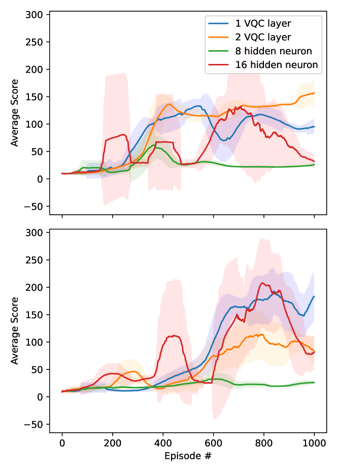
Fig. 5: Results: Quantum DRQN in Cart-Pole environment.

Fully Observable Cart-Pole  We first consider the standard setting that the RL agent can observe the full state of the environment. In Cart-Pole environment, this is a $4$-dimensional vector includes position and velocities as described in Section 6.1. The results are shown in the upper panel of Figure 5. We can observe that among the four cases we consider here: QLSTM with 1 or 2 VQC layers and LSTM with 8 or 16 hidden neurons, the QLSTM model with 2 VQC layers achieve the best performance. The QLSTM model with 1 VQC layer performs slightly worse than the one with two VQC layers. We also observe that, under the same training hyperparameters, the quantum models perform much better than their classical counterparts in both the stability and average scores.
Partially Observable Cart-Pole  We further consider the setting that the RL agent can only observe part of the state of the environment. In Cart-Pole environment, we reduce one dimension of the observation by dropping the last element in the observation vector. Now the RL agent can only get limited information from the environment. The task is more challenging than the previous one since the RL agent needs to figure out how to generate the decision based on partial information. The (Q)LSTM here may be more crucial because the agent may need information from previous steps. We observe that (in the lower panel of Figure 5), compared to the fully observed one, in the partially observed environment, the RL agent learns slower (requires more training episodes to reach high scores). Consistent with the fully observed cases, the quantum models perform better than their classical counterparts in both the stability and average scores. For example, the classical LSTM with 16 hidden neurons collapses after 800 episodes of training while the QLSTM agents remain stable.

7 Conclusions

In this paper, we first show the quantum recurrent neural network (QRNN)-based RL. Specifically, we employ the QLSTM as the $Q$-function approximator to realize the quantum deep recurrent $Q$-learning. From the results obtained from the testing environments we consider, our proposed framework shows higher stability and average scores than their classical counterparts when the model sizes are similar and training hyperparameters are fixed. The proposed method paves a new way of pursuing QRL with memory of previous time steps.

References

- [1] Michael A Nielsen and Isaac L Chuang, “Quantum computation and quantum information,” 2010.
- [2] John Preskill, “Quantum computing in the nisq era and beyond,” Quantum, vol. 2, pp. 79, 2018.
- [3] Kishor Bharti, Alba Cervera-Lierta, Thi Ha Kyaw, Tobias Haug, Sumner Alperin-Lea, Abhinav Anand, Matthias Degroote, Hermanni Heimonen, Jakob S Kottmann, Tim Menke, et al., “Noisy intermediate-scale quantum algorithms,” Reviews of Modern Physics, vol. 94, no. 1, pp. 015004, 2022.
- [4] Volodymyr Mnih, Koray Kavukcuoglu, David Silver, Andrei A Rusu, Joel Veness, Marc G Bellemare, Alex Graves, Martin Riedmiller, Andreas K Fidjeland, Georg Ostrovski, et al., “Human-level control through deep reinforcement learning,” nature, vol. 518, no. 7540, pp. 529–533, 2015.
- [5] David Silver, Julian Schrittwieser, Karen Simonyan, Ioannis Antonoglou, Aja Huang, Arthur Guez, Thomas Hubert, Lucas Baker, Matthew Lai, Adrian Bolton, et al., “Mastering the game of go without human knowledge,” nature, vol. 550, no. 7676, pp. 354–359, 2017.
- [6] Daoyi Dong, Chunlin Chen, Hanxiong Li, and Tzyh-Jong Tarn, “Quantum reinforcement learning,” IEEE Transactions on Systems, Man, and Cybernetics, Part B (Cybernetics), vol. 38, no. 5, pp. 1207–1220, 2008.
- [7] Samuel Yen-Chi Chen, Chao-Han Huck Yang, Jun Qi, Pin-Yu Chen, Xiaoli Ma, and Hsi-Sheng Goan, “Variational quantum circuits for deep reinforcement learning,” IEEE Access, vol. 8, pp. 141007–141024, 2020.
- [8] Owen Lockwood and Mei Si, “Reinforcement learning with quantum variational circuit,” in Proceedings of the AAAI Conference on Artificial Intelligence and Interactive Digital Entertainment, 2020, vol. 16, pp. 245–251.
- [9] Andrea Skolik, Sofiene Jerbi, and Vedran Dunjko, “Quantum agents in the gym: a variational quantum algorithm for deep q-learning,” Quantum, vol. 6, pp. 720, 2022.
- [10] Chih-Chieh CHEN, Koudai SHIBA, Masaru SOGABE, Katsuyoshi SAKAMOTO, and Tomah SOGABE, “Hybrid quantum-classical ulam-von neumann linear solver-based quantum dynamic programing algorithm,” Proceedings of the Annual Conference of JSAI, vol. JSAI2020, pp. 2K6ES203–2K6ES203, 2020.
- [11] Dirk Heimann, Hans Hohenfeld, Felix Wiebe, and Frank Kirchner, “Quantum deep reinforcement learning for robot navigation tasks,” arXiv preprint arXiv:2202.12180, 2022.
- [12] Sofiene Jerbi, Casper Gyurik, Simon Marshall, Hans J Briegel, and Vedran Dunjko, “Variational quantum policies for reinforcement learning,” arXiv preprint arXiv:2103.05577, 2021.
- [13] Jen-Yueh Hsiao, Yuxuan Du, Wei-Yin Chiang, Min-Hsiu Hsieh, and Hsi-Sheng Goan, “Unentangled quantum reinforcement learning agents in the openai gym,” arXiv preprint arXiv:2203.14348, 2022.
- [14] Michael Schenk, Elías F Combarro, Michele Grossi, Verena Kain, Kevin Shing Bruce Li, Mircea-Marian Popa, and Sofia Vallecorsa, “Hybrid actor-critic algorithm for quantum reinforcement learning at cern beam lines,” arXiv preprint arXiv:2209.11044, 2022.
- [15] Qingfeng Lan, “Variational quantum soft actor-critic,” arXiv preprint arXiv:2112.11921, 2021.
- [16] André Sequeira, Luis Paulo Santos, and Luís Soares Barbosa, “Variational quantum policy gradients with an application to quantum control,” arXiv preprint arXiv:2203.10591, 2022.
- [17] Won Joon Yun, Yunseok Kwak, Jae Pyoung Kim, Hyunhee Cho, Soyi Jung, Jihong Park, and Joongheon Kim, “Quantum multi-agent reinforcement learning via variational quantum circuit design,” arXiv preprint arXiv:2203.10443, 2022.
- [18] Samuel Yen-Chi Chen, Chih-Min Huang, Chia-Wei Hsing, Hsi-Sheng Goan, and Ying-Jer Kao, “Variational quantum reinforcement learning via evolutionary optimization,” Machine Learning: Science and Technology, vol. 3, no. 1, pp. 015025, 2022.
- [19] Shaojun Wu, Shan Jin, Dingding Wen, and Xiaoting Wang, “Quantum reinforcement learning in continuous action space,” arXiv preprint arXiv:2012.10711, 2020.
- [20] Richard S Sutton and Andrew G Barto, Reinforcement learning: An introduction, MIT press, 2018.
- [21] Matthew Hausknecht and Peter Stone, “Deep recurrent q-learning for partially observable mdps,” in 2015 aaai fall symposium series, 2015.
- [22] Abhinav Kandala, Antonio Mezzacapo, Kristan Temme, Maika Takita, Markus Brink, Jerry M Chow, and Jay M Gambetta, “Hardware-efficient variational quantum eigensolver for small molecules and quantum magnets,” Nature, vol. 549, no. 7671, pp. 242–246, 2017.
- [23] Edward Farhi, Jeffrey Goldstone, and Sam Gutmann, “A quantum approximate optimization algorithm,” arXiv preprint arXiv:1411.4028, 2014.
- [24] Jarrod R McClean, Jonathan Romero, Ryan Babbush, and Alán Aspuru-Guzik, “The theory of variational hybrid quantum-classical algorithms,” New Journal of Physics, vol. 18, no. 2, pp. 023023, 2016.
- [25] Sukin Sim, Peter D Johnson, and Alán Aspuru-Guzik, “Expressibility and entangling capability of parameterized quantum circuits for hybrid quantum-classical algorithms,” Advanced Quantum Technologies, vol. 2, no. 12, pp. 1900070, 2019.
- [26] Trevor Lanting, Anthony J Przybysz, A Yu Smirnov, Federico M Spedalieri, Mohammad H Amin, Andrew J Berkley, Richard Harris, Fabio Altomare, Sergio Boixo, Paul Bunyk, et al., “Entanglement in a quantum annealing processor,” Physical Review X, vol. 4, no. 2, pp. 021041, 2014.
- [27] Yuxuan Du, Min-Hsiu Hsieh, Tongliang Liu, and Dacheng Tao, “The expressive power of parameterized quantum circuits,” arXiv preprint arXiv:1810.11922, 2018.
- [28] Amira Abbas, David Sutter, Christa Zoufal, Aurélien Lucchi, Alessio Figalli, and Stefan Woerner, “The power of quantum neural networks,” Nature Computational Science, vol. 1, no. 6, pp. 403–409, 2021.
- [29] Matthias C Caro, Hsin-Yuan Huang, Marco Cerezo, Kunal Sharma, Andrew Sornborger, Lukasz Cincio, and Patrick J Coles, “Generalization in quantum machine learning from few training data,” Nature communications, vol. 13, no. 1, pp. 1–11, 2022.
- [30] Kosuke Mitarai, Makoto Negoro, Masahiro Kitagawa, and Keisuke Fujii, “Quantum circuit learning,” Physical Review A, vol. 98, no. 3, pp. 032309, 2018.
- [31] Jun Qi, Chao-Han Huck Yang, and Pin-Yu Chen, “Qtn-vqc: An end-to-end learning framework for quantum neural networks,” arXiv preprint arXiv:2110.03861, 2021.
- [32] Mahdi Chehimi and Walid Saad, “Quantum federated learning with quantum data,” in ICASSP 2022-2022 IEEE International Conference on Acoustics, Speech and Signal Processing (ICASSP). IEEE, 2022, pp. 8617–8621.
- [33] Samuel Yen-Chi Chen and Shinjae Yoo, “Federated quantum machine learning,” Entropy, vol. 23, no. 4, pp. 460, 2021.
- [34] Samuel Yen-Chi Chen, Chih-Min Huang, Chia-Wei Hsing, and Ying-Jer Kao, “An end-to-end trainable hybrid classical-quantum classifier,” Machine Learning: Science and Technology, vol. 2, no. 4, pp. 045021, 2021.
- [35] Chao-Han Huck Yang, Jun Qi, Samuel Yen-Chi Chen, Pin-Yu Chen, Sabato Marco Siniscalchi, Xiaoli Ma, and Chin-Hui Lee, “Decentralizing feature extraction with quantum convolutional neural network for automatic speech recognition,” in ICASSP 2021-2021 IEEE International Conference on Acoustics, Speech and Signal Processing (ICASSP). IEEE, 2021, pp. 6523–6527.
- [36] Chao-Han Huck Yang, Jun Qi, Samuel Yen-Chi Chen, Yu Tsao, and Pin-Yu Chen, “When bert meets quantum temporal convolution learning for text classification in heterogeneous computing,” in ICASSP 2022-2022 IEEE International Conference on Acoustics, Speech and Signal Processing (ICASSP). IEEE, 2022, pp. 8602–8606.
- [37] Riccardo Di Sipio, Jia-Hong Huang, Samuel Yen-Chi Chen, Stefano Mangini, and Marcel Worring, “The dawn of quantum natural language processing,” in ICASSP 2022-2022 IEEE International Conference on Acoustics, Speech and Signal Processing (ICASSP). IEEE, 2022, pp. 8612–8616.
- [38] Samuel Yen-Chi Chen, Shinjae Yoo, and Yao-Lung L Fang, “Quantum long short-term memory,” in ICASSP 2022-2022 IEEE International Conference on Acoustics, Speech and Signal Processing (ICASSP). IEEE, 2022, pp. 8622–8626.
- [39] Johannes Bausch, “Recurrent quantum neural networks,” arXiv preprint arXiv:2006.14619, 2020.
- [40] Sepp Hochreiter and Jürgen Schmidhuber, “Long short-term memory,” Neural computation, vol. 9, no. 8, pp. 1735–1780, 1997.
- [41] Greg Brockman, Vicki Cheung, Ludwig Pettersson, Jonas Schneider, John Schulman, Jie Tang, and Wojciech Zaremba, “Openai gym,” arXiv preprint arXiv:1606.01540, 2016.