Anisotropic multiresolution analyses for deepfake detection

Abstract

Generative Adversarial Networks (GANs) have paved the path towards entirely new media generation capabilities at the forefront of image, video, and audio synthesis. However, they can also be misused and abused to fabricate elaborate lies, capable of stirring up the public debate. The threat posed by GANs has sparked the need to discern between genuine content and fabricated one. Previous studies have tackled this task by using classical machine learning techniques, such as k-nearest neighbours and eigenfaces, which unfortunately did not prove very effective. Subsequent methods have focused on leveraging on frequency decompositions, i.e., discrete cosine transform, wavelets, and wavelet packets, to preprocess the input features for classifiers. However, existing approaches only rely on isotropic transformations. We argue that, since GANs primarily utilize isotropic convolutions to generate their output, they leave clear traces, their fingerprint, in the coefficient distribution on sub-bands extracted by anisotropic transformations. We employ the fully separable wavelet transform and multiwavelets to obtain the anisotropic features to feed to standard CNN classifiers. Lastly, we find the fully separable transform capable of improving the state-of-the-art.

1 Introduction

Generative Adversarial Networks (GANs) have become a thriving topic in recent years after the initial work by Goodfellow et al.in [16]. Since then, GANs have quickly become a popular and rapidly changing field due to their ability to learn high-dimensional complex real image distributions. As a result, numerous GAN variants have emerged, like CramerGAN ([5]), MMDGAN ([26]), ProGAN ([14]), SN-DCGAN ([33]), and the state-of-the-art StyleGAN, StyleGAN2, and StyleGAN3 ([22, 23, 21]). Among various primary applications of GANs is fake image and video generation, e.g., Deepfakes ([1]), FaceApp ([2]), and ZAO ([3]). In particular, Deepfakes is the first successful project taking advantages of deep learning, which was started in 2017 on Reddit by an account with the same name. Since then, deepfakes are regarded as falsified images and videos created by deep learning algorithms, see [39]. A major source of motivation for investigation into the automatic deepfake detection is the visual indistinguishability between fake images created by GANs and real ones. Moreover, the abuse of fake images potentially pose threats to personal and national security. Therefore, research on deepfake detection has become increasingly important with the rapid iteration of GANs.

There are two kinds of tasks in the detection of GAN-generated images. The easiest is identifying an image as real or fake. The harder one consists of attributing fake images to the corresponding GAN that generated them. In this paper, we mainly focus on the attribution task. Both tasks involve extracting features from images and feeding them to classifiers. For the classifiers, there are approaches based on traditional machine learning methods, which are relatively simple, but often reach relatively bad results, see [13, 24]. Approaches based on deep learning, especially convolutional neural networks (CNN), have proven powerful and are employed in many recent papers, see [38, 45, 42, 28, 47, 12, 43]. For feature extraction, the simplest method is just using raw pixels as input. The results are, however, not of high accuracy and the classifiers fed with raw pixels are not robust under common perturbations, see [28, 12]. Therefore, it is necessary to develop methods to better extract features. One stream is the learning-based method by Yu et al.in [45, 46, 47], which found unique fingerprints of each GAN. Another stream is based on the mismatches between real and fake in the frequency domain, see [48, 10, 12, 9, 28, 43]. Specifically, multiresolution methods, e.g., the wavelet packet transform, have recently been employed for deepfake detection, see Wolter et al.in [43]. Their work demonstrates the capabilities of multiresolution analyses for the task at hand and marks the starting point for our considerations. In contrast to the isotropic transformations considered there, we focus on anisotropic transformations, i.e., the fully separable wavelet transform ([40]) and samplets ([18]), which are a particular variant of multiwavelets.

Because the generators in all GAN architectures synthesize images in high resolution from low resolution images using deconvolution layers with square sliding windows, it is highly likely for the anisotropic multi wavelet transforms of fake images to leave artifacts on anisotropic sub-bands. In this paper, we show that features from anisotropic (multi-)wavelet transforms are promising descriptors of images. This is due to remarkable mismatches between the anisotropic multiwavelet transforms of real and fake images, see Figure 3. To evaluate the anisotropic features, we set up a lightweight multi-class CNN classifier as in [12, 43] and compare our results on the datasets consisting of authentic images from one of the three commonly used image datasets: Large-scale Celeb Faces Attributes (CelebA [27]), LSUN bedrooms ([44]), and Flickr-Faces-HQ (FFHQ [22]), and synthesized images generated by CramerGAN, MMDGAN, ProGAN, and SN-DCGAN on the CelebA and LSUN bedroom, or the StyleGANs on the FFHQ. Finally, as in [12, 43], we test the sensitivity to the number of training samples and the robustness under the four common perturbations: Gaussian blurring, image crop, JPEG based compression, and addition of Gaussian noise.

2 Related work

Deepfake detection: A comprehensive statistical studying of natural images shows that regularities always exist in natural images due to the strong correlations among pixels, see [29]. However, such regularity does not exist in synthesized images. Besides, it is well-known that checkerboard artifacts exist in CNNs-generated images due to downsampling and upsampling layers, see examples in [37, 4]. The artifacts make identification of deepfakes possible. In [31, 38, 42], the authors show that GAN-generated fake images can be detected using CNNs fed by conventional image foresics features, i.e., raw pixels. In order to improve the accuracy and generalization of classifier, several methods are proposed to address the problem of finding more discriminative features instead of raw pixels. Several non-learnable features are proposed, for example hand-crafted cooccurrence features in [35], color cues in [32], layer-wise neuron behavior in [41], and global texture in [28]. In [45], Yu et al.discover the possibility of uniquely fingerprinting each GAN model and characterize the corresponding output during the training procedure. With this technique, responsible GAN developers could fingerprint their models and keep track of abnormal usage of their releases. In the follow-up paper ([47]), Yu et al.scale up the GAN fingerprinting mechanism. However, in [36], Neves et al.propose GANprintR to remove the fingerprints of GANs, which renders this identification method useless.

Frequency artifacts: It is found that artifacts are more visible in the frequency domain. State of the art results are achieved using features in the frequency domain, e.g., the coefficients of the discrete cosine transform ([48, 10, 12, 9, 28]) and the coefficients of the isotropic wavelet packet transform ([43]). In [12], Frank et al.found that the grid-like patterns in the frequency domain stem from the upsampling layers. Even though ProGAN and StyleGANs are equipped with improved upsampling methods, artifacts still exit in their frequency domain. Combination of the features in frequency domain and lightweight convolutional neural networks can outperform the complex heavyweight convolution neural networks using features based on the pixel values of images. In [43], features based on wave-packets are used, which outperforms all the other state-of-the-art methods with comparable lightweight CNN classifiers. The success of the isotropic wave-packets inspired us to further investigate this direction and to also take into account anisotropic multiresolution analyses, to extract more distinguishable features for the deepfake detection.

3 Proposed Method

3.1 Motivation

Images are often composed of two types of regions: mostly monochromatic patches, usually backgrounds, and areas with sharp color gradients, found in correspondence with borders that separate different objects. This construction is similar to a square wave in 1D, which is notoriously difficult to approximate with only cosine functions like the discrete cosine transform (DCT) does. This fact is known as the Gibbs phenomenon, see [15]. Similar to a square wave in 1D, images can be considered as piecewise constant functions in 2D, which makes using DCT methods challenging as their supports are not localized in space but only in frequency. This results in redundant representations of images in the frequency domain. One solution, proposed in [43], is to decompose an image into frequencies while also maintaining spatial information is using wavelets, which are localized in both domains and are thus less susceptible to discontinuities. In order to manifest the efficient representation of images using wavelets, we consider an isotropic pattern with discontinuities on the boundaries of square blocks, and a anisotropic pattern with discontinuities on the boundaries of rectangular blocks, see Figure 1. We then compute the DCT and four different kinds of wavelet transforms, i.e., the discrete wavelet transform (DWT), the discrete wavelet packet transform (DWPT), the fully separable wavelet transform (FSWT), and the samplet transform. From the bar plot in Figure 1, all wavelet transforms overcome the Gibbs phenomenon, in contrast to the DCT. However, anisotropic wavelet transforms, i.e., FSWT and samplets, perform much better than isotropic DWT and DWPT in the task of finding efficient representations for anisotropic patterns which commonly exist in real images.

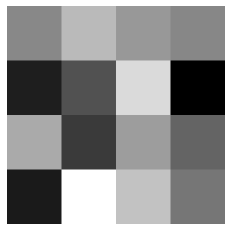
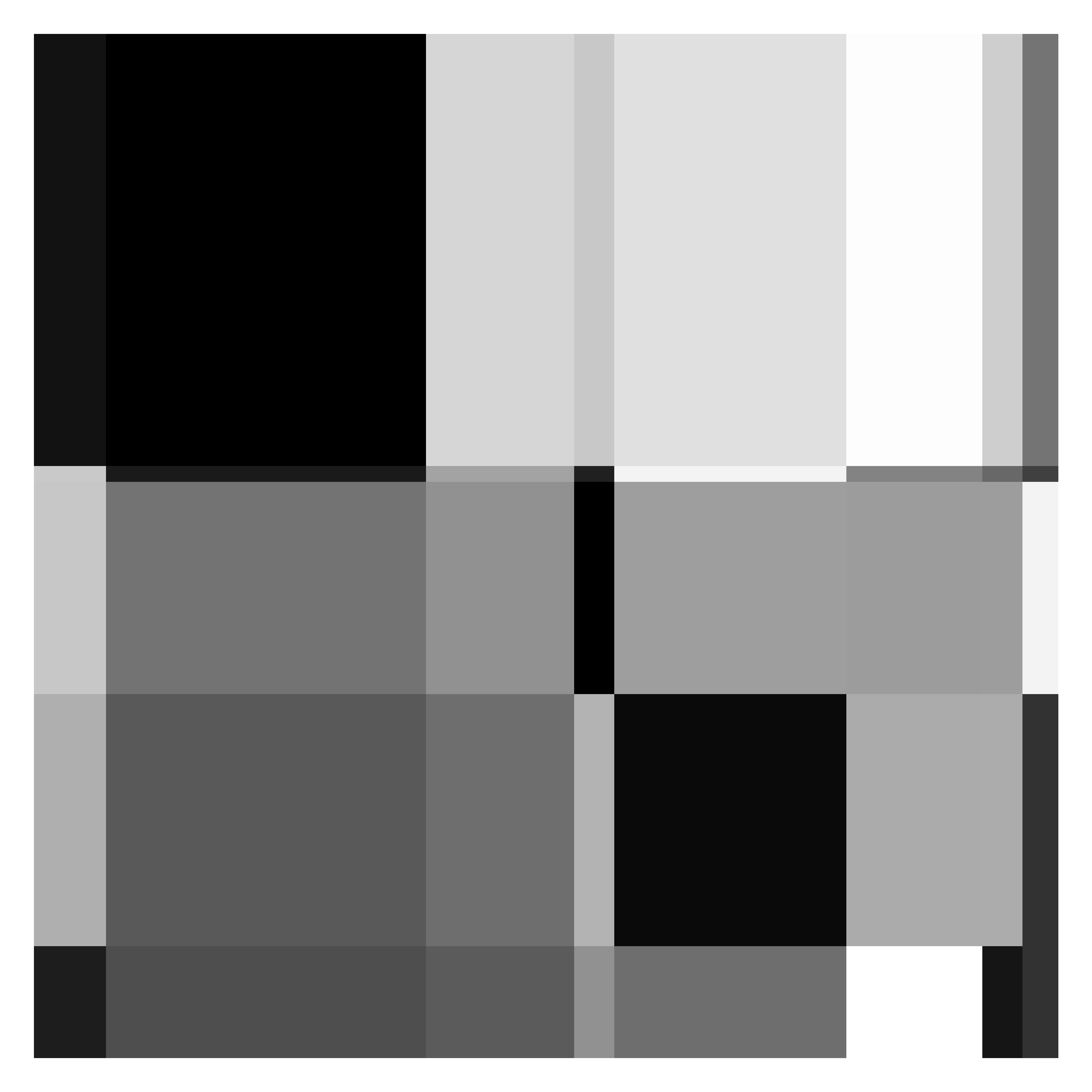
Figure 1: The top left part shows a $256\times 256$ blockwise constant grayscale image with 16 squares of equal size (black stands for 0, and white stands for 255). The bottom left part shows a $256\times 256$ blockwise constant grayscale image with 40 rectangles (black stands for 0, and white stands for 255). The right part shows the numbers of nonzero coefficients under different transforms of the isotropic and anisotropic patterns respectively. Herein, we consider the wavelets and samplets with vanishing moments up to order 1.

The previous works [48, 12] have already analyzed the effectiveness of using the frequency domain instead of the direct pixel representation when detecting deepfakes. Moreover, the method in [43] has improved the state-of-the-art result using the isotropic wavelet, i.e., the DWPT. However, they usually result in redundant representations of images. Moreover, they rely on only isotropic decompositions. We are convinced that anisotropic transforms can add a new aspect to the challenge at hand. The intuition behind this reasoning comes from the fact that GAN architectures typically only use isotropic convolutions (square sliding windows) to synthesize new samples, thus being unaware of the fingerprint they are leaving in the hidden anisotropic coefficients’ distribution of the image.

We focus on two technologies that allow us to expose these fingerprints and obtain a spatio-frequency representation of the source image: the fully separable wavelet transform and samplets, which are a particular variant of multiwavelets.

3.2 Preliminaries

3.2.1 Isotropic wavelets

Discrete wavelet transform: Wavelets are localized waves that have a nonzero value around a certain point but then collapse to zero when moving further away. Examples for such wavelets are Haar- and Daubechies- wavelets, see [8]. The main idea behind wavelet-based analyses is the decomposition of a signal with respect to a hierarchical scales. The smaller the scales, the higher the corresponding frequency. Unlike the DCT, wavelets are localized in the spatial domain as well, due to their hierarchical nature. The fast wavelet transform (FWT), see [6], is an algorithm commonly used to apply a discrete wavelet transform onto an $n\times n$ image and decompose it into approximation coefficients using convolutions of filter banks and downsampling operators, with a computational cost in the order of $\mathrm{O}(n^{2})$, i.e., linear in the number of pixels. The results of one decomposition step of the FWT are four sets of coefficients usually referred to as $a$, $h$, $v$, $d$, which stand for approximation, horizontal, vertical, and diagonal coefficients. To produce a decomposition up to level $l$, the $a$ coefficient of level $l-1$ is further decomposed into four components: $aa$, $ah$, $av$, $ad$, giving rise to the structure in the leftmost side of Figure 2. This approach is also known as Mallat decomposition ([30]) and amounts to a 2D isotropic wavelet transform. All frequency-based methods like Fourier transformations and wavelets are usually tailored towards unbounded domains, while images are instead bounded. In the case of the Haar wavelet, the transition from unbounded to bounded is not a problem and no boundary modifications are required to obtain an orthonormal basis. However, higher-order wavelets require modifications at the boundary, which introduces the need for padding, usually accomplished either by appending zeros to a dimension or by repeating the data or reflecting it. To avoid changing the size of images, the Gram-Schmidt boundary filter is proposed in [20], which replaces the wavelet filters at the boundary with special shorter filters that preserve both the shape and the reconstruction property of the wavelet transform.

Wavelet packets: Following the assumption that information is mostly contained in the low-frequency approximation coefficient $a$, the Mallat approach leaves the high frequency terms $h$, $v$, and $d$ untouched when moving up one level in the decomposition. Previous work ([11]) has instead shown that, especially when dealing with compressed and lower resolution images, information in the higher frequencies is usually affected more by the reduction processes than that in the lower part of the frequency spectrum. Therefore, the remaining three feature maps are likely to also contain relevant information for deepfake detection. Motivated by this reasoning, the authors of [43] employed wavelet packets as input features for their classifiers. A single level decomposition of a wavelet packet is essentially the same as that of the FWT, but when decomposing up to level $l$, also the $h$, $v$, and $d$ of level $l-1$ are further decomposed into $(ha,hh,hv,hd)$, $(va,vh,vv,vd)$ and $(da,dh,dv,dd)$, at the total cost of $\mathrm{O}(n^{2}\log n)$ operations. The resulting quad-tree-like structure is depicted in the middle of Figure 2 for a complete decomposition. In [43], the authors used a Gram-Schmidt boundary filter such that coefficients of any image using the wavelet packet transform remain the same size as the transformed image. Afterwards, all packets are stacked together along the channel direction before feeding the CNN.

Figure 2: Leftmost: the quad tree structure of the wavelet decomposition of an image. Middle: the complete tree structure of a wavelet packet. Rightmost: tree structure of a fully separable wavelet decomposition.

3.2.2 Anisotropic wavelets

Fully Separable Wavelet Transform: Previous work has focused on the isotropic discrete wavelet transform and its derivatives to extract features. For images, the isotropic decomposition from level 1 up to level $l$ consists of transforming each axis once for each level. As we have seen with the FWT and wavelet packets, first the $x$ axis is decomposed, then the $y$ axis, and only after the algorithm moves to the next level. Instead, the fully separable decomposition first decomposes completely one axis up to level $l$ and then decomposes the obtained features on the other axis (see the rightmost of Figure 2 for a sketch of the resulting pattern). This different approach gives rise to a more anisotropy-friendly feature extraction while only increasing the computational cost by a factor of two compared to the Mallat decomposition. Similarly to wavelet packets, a suitable boundary modification, e.g., by padding, is necessary for the fully separable wavelet transform with more than one vanishing moment. In this paper, we consider both the reflect-padding method and the boundary filter with QR orthogonalization.

Samplets: First presented in [18], samplets are a generalization of multiwavelets that produce a multiresolution analysis of a given signal in terms of discrete signed measures. Samplets can be constructed with an arbitrary number $m$ of vanishing moments for arbitrary data sets. For structured data, such as images, lowest order samplets (m=1) correspond to Haar wavelets. The construction of the basis and the fast samplet transform can both be performed in linear time, i.e., the cost of transforming an $n\times n$ input image is $\mathcal{O}(n^{2})$. Different from the FSWT, samplets are a data-centric approach and can accommodate any data dimensions without the need for padding or special boundary treatment. In particular, they do not suffer from discontinuities at the boundaries and do not introduce artifacts in the decomposition, which allows using samplets directly without modifications and without increasing their computational cost.

3.3 Proof of concept

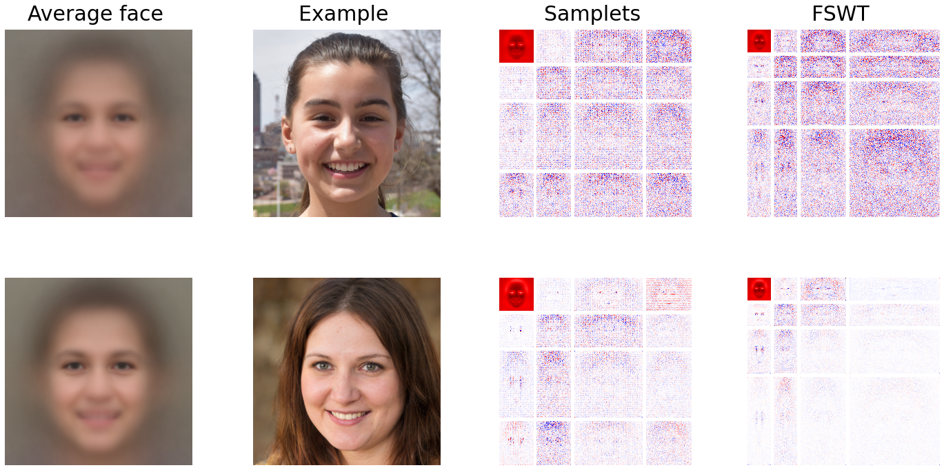
Figure 3: A row by row comparison of real and synthesized images on sub-bands. The first row shows the average of 1000 real images from the FFHQ dataset. The second column shows the corresponding block-wise normalized samplet coefficients, while the last column shows the block-wise normalized coefficients of the FSWT. Herein, we employed samplets with vanishing moments up to order $3$ and level $l=3$, and the FSWT with the Daubechies 3 orthogonal wavelet, reflect-padding method, and $l=3$. The second row shows the same information for a dataset of the same size generated by the StyleGAN model taken from thispersondoesnotexist.com. In the color map, white stands for zeros, red for positive numbers, and blue for negative numbers.

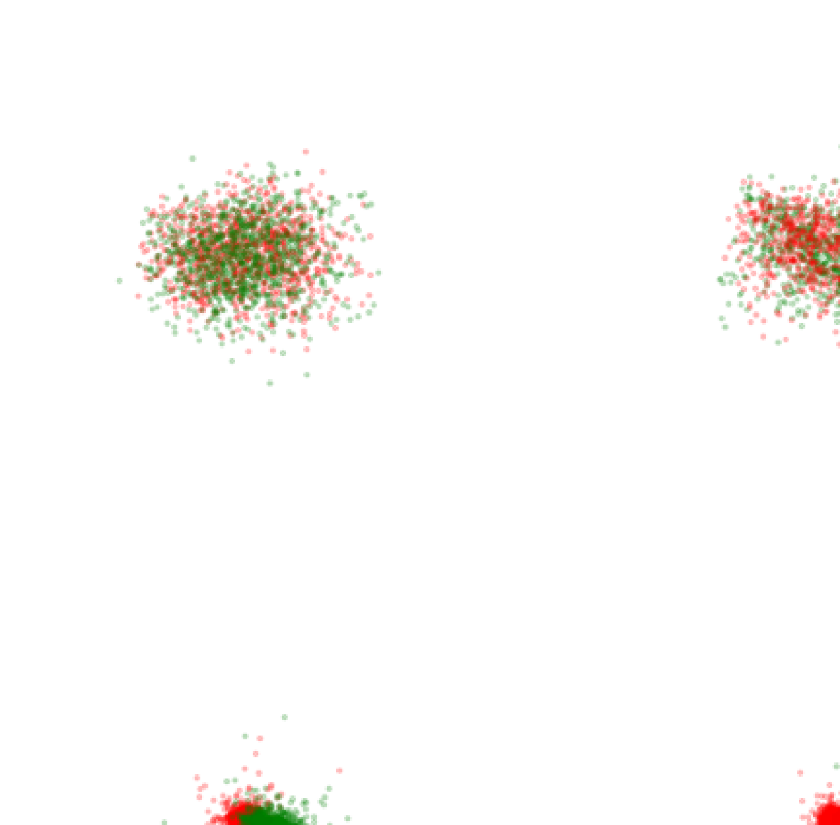
(a) Raw pixels

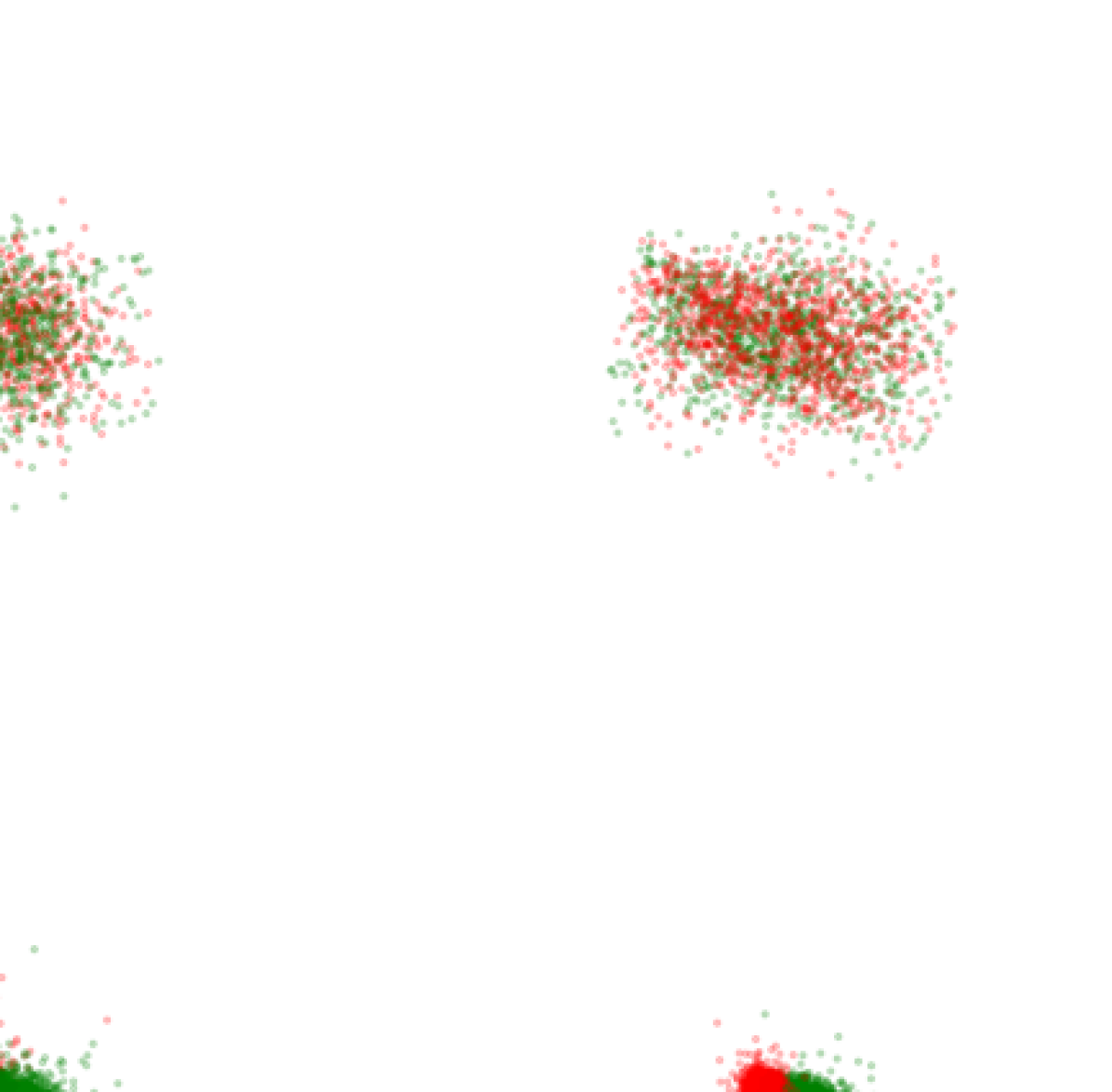
(b) Low frequency coefficients

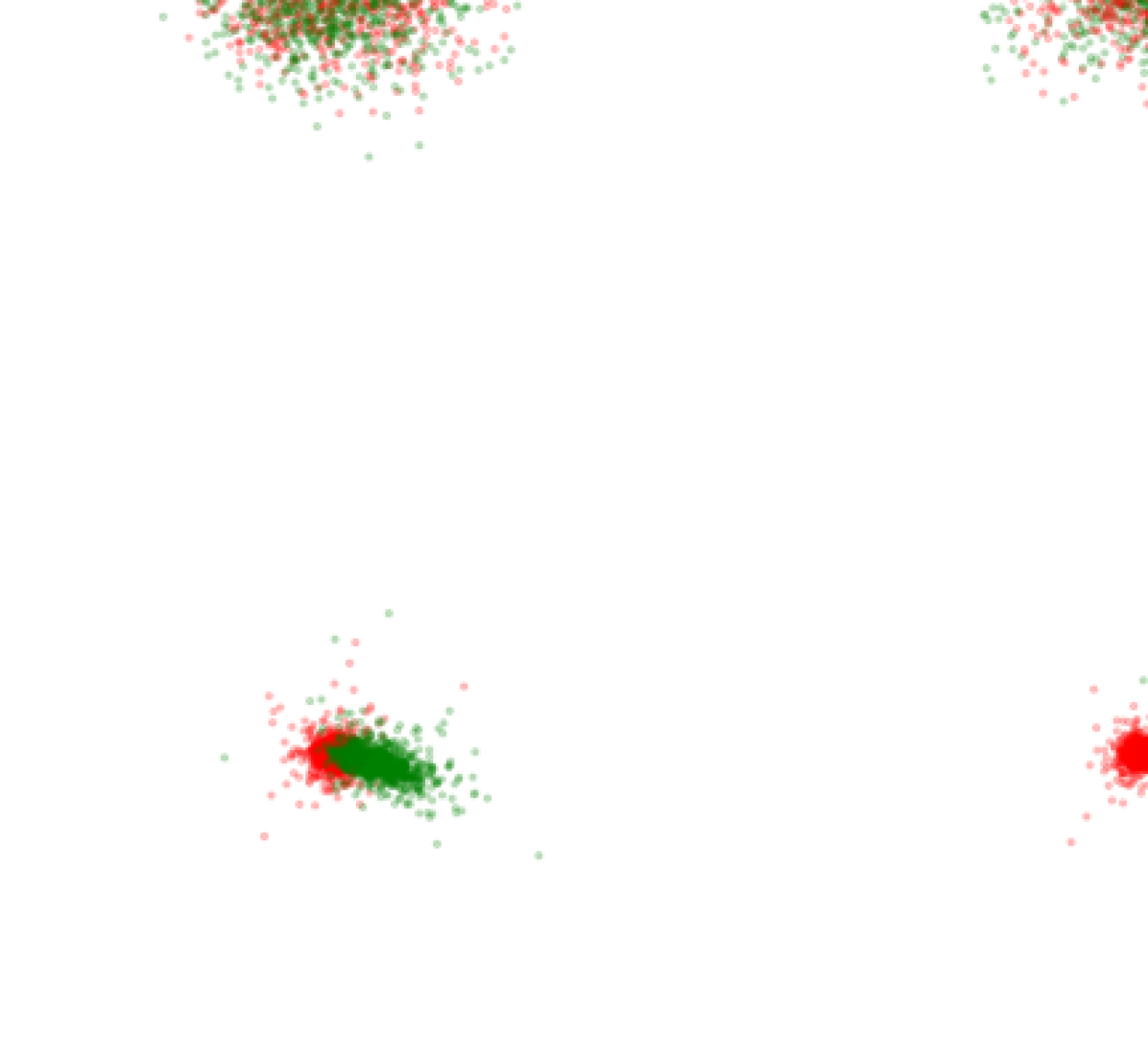
(c) Anisotropic coefficients

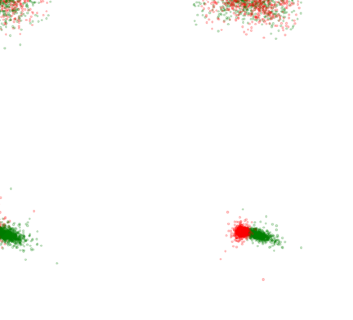
(d) High frequency coefficients

Figure 4: The 3D scatter plots of 2000 samples consisting of 1k real and 1k fake images visualize the first three principle components of the raw pixels and the three different parts of the FSWT coefficients.The red nodes represent real images, and the green ones represent fake images.

To illustrate how features are extracted by anisotropic multiresolution analyses, we visualize in Figure 3 the samplet- and FSTW- coefficients for the average of 1000 real images from the FFHQ (top row) and for 1000 images by the StyleGAN models from the photorealistic face generation website thispersondoesnotexist.com (bottom row). As can be seen, the average images from the real sample and the one generated by StyleGAN in the first column are very similar. In particular, it is very difficult to tell which of the exemplary images in the second column is synthesized and which one is real. According to the experiments in [28], human performance in classification only leads to an accuracy of about 63.9% in the FFHQ vs StyleGAN case, which is only slightly higher than the probability of randomly guessing. The two anisotropic transforms lead to the sparse patterns on the right side of the figure. The patterns for the real images and the synthesized images are clearly distinguishable, especially by examining the high and anisotropic frequency parts. These observations suggest that samplets and FSWT are suitable for assisting classifiers in discerning the origin of a given image.

To further illustrate the idea of using features extracted by the two proposed anisotropic transforms, we visualize the first three principal components of the raw pixels and different parts of the FSWT coefficients in a principal component analysis (PCA). The samples for FFHQ and StyleGAN2 consist of 1000 images, each, with a resolution of $128\times 128$. Panel (a) in Figure 4 shows the principal components of the raw pixels, which are not distinguishable. The same accounts for the low frequency contributions depicted in panel (b). In turn, the principal components of real and synthesized images become linearly separable in the anisotropic parts and high frequency parts, depicted in panels (c) and (d).

The scales of the wavelet transform coefficients decrease exponentially with respect to their underlying level $l$ if the underlying signal exhibits sufficient smoothness. However, the importance of the high frequency coefficients at high levels is large. Therefore, we employ a block-wise normalization, where we divide coefficients by the maximum absolute value on the corresponding block. This way, we can bring each block to the same range $(-1,1)$. Moreover, we keep the zero coefficients untouched to maintain the sparsity pattern. In the following experiments, this block-wise normalization is always applied before feeding the data into the CNN classifier.

4 Experiments

All experiments in this paper are performed on a compute server with two Intel Xeon (E5-2650 v3 @ 2.30GHz), one NVIDIA A100-PCIe-40GB, two NVIDIA GeForce GTX 1080 Ti (Titan 11GB GDDR5X), and one NVIDIA GeForce GTX 1080 (Founders Edition 8GB GDDR5X).

4.1 Source Identification

Experimental Setup The experiments are conducted on three datasets: CelebA, LSUN bedroom, and FFHQ. The datasets CelebA and LSUN bedroom are generated by the pre-trained GAN models from [45], and contain 150k resized real images of resolution $128\times 128$ and 150k fake images in the same size for each model. The models under consideration are CramerGAN, MMDGAN, ProGAN, and SN-DCGAN. Thus, the total dataset has a size of 750k. It is then partitioned into training, validation, and test datasets consisting of 500k, 100k, and 150k images respectively. On the other hand, the FFHQ dataset contains 70k real images resized to $128\times 128$ and 70k fake images of the same size for each StyleGAN model, i.e., StyleGAN, StyleGAN2, and StyleGAN3. As in [43], we split the full dataset into training, validation, and test datasets with sizes of 252k, 8k, and 20k, respectively. The CelebA and LSUN bedroom samples are generated following the recommendations of the from the references [12, 43], which suggest using the pre-trained models from [45]. Analogously to [43], the fake dataset of FFHQ is instead generated using the pre-trained models provided by the authors of [22, 23, 21], using, in particular, the R configuration (translation and rotation equivalent) of StyleGAN3, a value of 1 for the truncation parameter, and image numbers from 1 to 70k as the random seeds.

Secondly, the fully separable wavelet transform is realized by using the GPU enabled fast wavelet transform library ptwt ([17, 34, 7]). The samplets, implemented in C++, are integrated into the toolchain by using pybind11 ([19]). The implementation is available at https://github.com/muchip/fmca.

In order to demonstrate the advantages of features extracted by anisotropic multiresolution analyses, we train the same shallow CNN proposed in [12], fed with the samplets and the fully separable decomposition to match the state of the art performance. In the architecture, a fully connected layer is added at the end of the convolution part as a classifier. Its output is the number of classes, and the input size is $32d^{2}$, where $d$ depends on the size of input features. Because the samplet transform does not involve any padding procedure, $d$ for the samplets is the same number as for the raw pixels. However, the size of the fully separable decomposition coefficients depends on the padding methods, which is slightly larger than the size of the raw pixels and the samplets except when using boundary filters. Therefore, the fully connected layer for the FSWT without the boundary method is slightly larger than that for the raw pixels and samplets. With a specific size for the Daubechies 3 orthogonal wavelet (db3), and reflect-padding method the total number of parameters for the FSWT increase to roughly 202k compared to the 170k parameters for the raw pixels, DCT, and samplets. Even though the numbers of parameters for samplets and FSWT are the same as for DCT and, thus, larger than for wavelet packets, their parameters are still only around $2\%$ of the parameters in [45]. Besides, the training and evaluation procedures are faster using samplets or FSWT compared to wavelet packets due to their linear time complexity.

In the training procedure, we set the batch size to 128 and train the model using the Adam algorithm ([25]) with a learning rate of 0.001 for 10 epochs. The random seed values used are 0,1,2,3,4 for 5 repetitive training procedures. The random seed is not only used to initialize the network weights, but also shuffle the entire datasets before splitting. This way, there is no bias in the partitioning of the data into the training, test, and validation datasets.

CelebA% LSUN bedrooms% Method complexity parameters max $\mu\pm\sigma$ max $\mu\pm\sigma$ Pixels (Frank et al.[12]) $\mathrm{O}(1)$ 170k 97.80 - 98.95 - DCT (Frank et al.[12]) $\mathrm{O}(n^{2}\log n)$ 170k 99.07 - 99.64 - Packet-ln-db3 (Wolter et al.[43]) $\mathrm{O}(n^{2}\log n)$ 109k 99.38 $99.11\pm 0.49$ 99.19 $99.01\pm 0.17$ Packet-ln-db4 (Wolter et al.[43]) $\mathrm{O}(n^{2}\log n)$ 109k 99.43 $99.27\pm 0.15$ 99.02 $98.46\pm 0.67$ Samplets-BN-2-3 (our) $\mathrm{O}(n^{2})$ 170k 99.84 $99.71\pm 0.12$ 99.49 $99.31\pm 0.15$ Samplets-BN-3-3 (our) $\mathrm{O}(n^{2})$ 170k 99.92 $99.86\pm 0.06$ 99.44 $99.36\pm 0.09$ Samplets-BN-4-3 (our) $\mathrm{O}(n^{2})$ 170k 99.79 $99.75\pm 0.06$ 99.2 $98.96\pm 0.21$ Samplets-BN-5-3 (our) $\mathrm{O}(n^{2})$ 170k 99.87 $99.79\pm 0.05$ 99.52 $99.34\pm 0.11$ Samplets-BN-6-3 (our) $\mathrm{O}(n^{2})$ 170k 99.87 $99.82\pm 0.04$ 99.55 $99.42\pm 0.13$ Samplets-BN-7-3 (our) $\mathrm{O}(n^{2})$ 170k 99.89 $99.77\pm 0.12$ 99.62 $99.38\pm 0.24$ FSWT-BN-db3-3-boundary (our) $\mathrm{O}(n^{2})$ 170k 99.88 $99.84\pm 0.05$ 99.1 $98.76\pm 0.35$ FSWT-BN-db4-3-boundary (our) $\mathrm{O}(n^{2})$ 170k 99.91 $99.76\pm 0.11$ 99.33 $99.13\pm 0.18$ FSWT-BN-db3-3-reflect (our) $\mathrm{O}(n^{2})$ 202k 99.97 $99.96\pm 0.01$ 99.9 $99.79\pm 0.06$ FSWT-BN-db4-3-reflect (our) $\mathrm{O}(n^{2})$ 225k 99.96 $99.86\pm 0.14$ 99.86 $99.79\pm 0.04$

Table 1: Accuracy results for different features with max, mean and standard deviation on the CelebA and the LSUN bedroom datasets. We report our results in comparison to the results in [12, 43], which are obtained using seeds from 0 to 4.

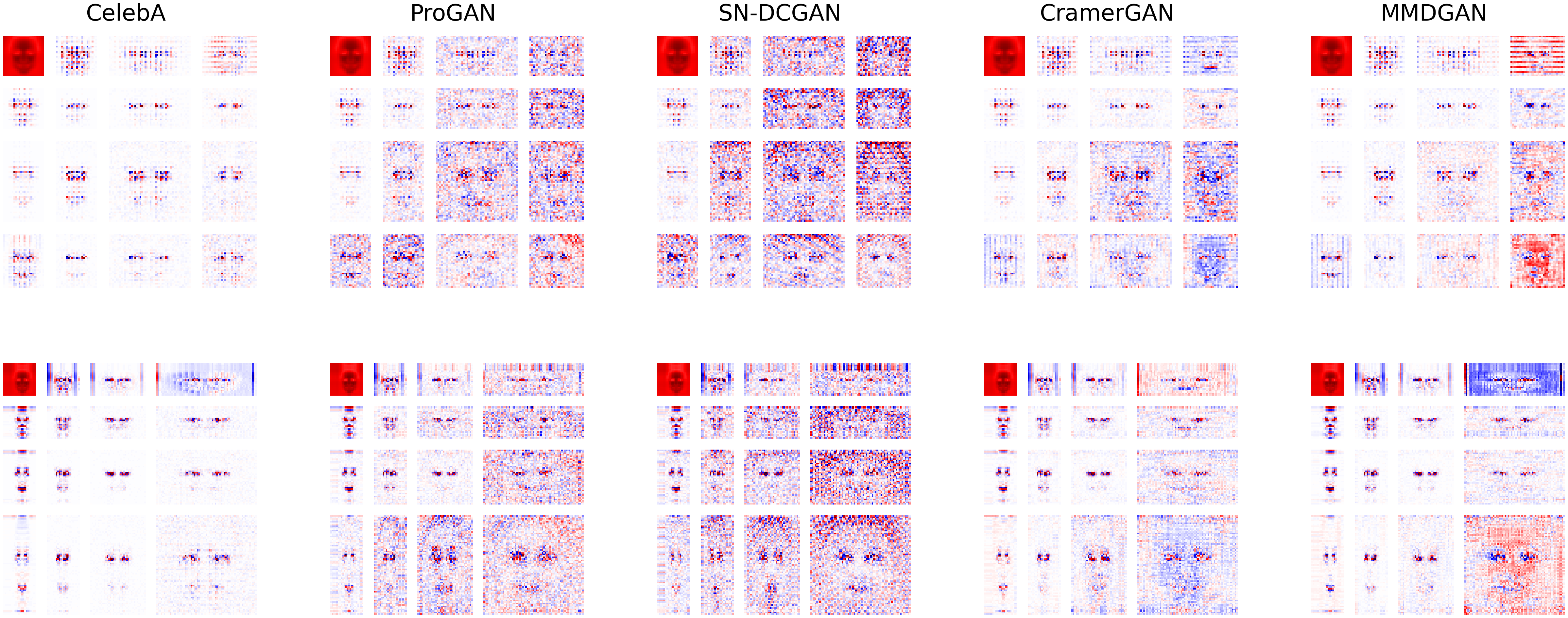
Figure 5: Average coefficients of each feature extraction method on the CelebA dataset. These visualizations are obtained by applying the block-wise normalization, then scaling them to the range $(0,255)$, and finally casting to unsigned int 8 bit. The first row corresponds Samplets-BN-3-3 and the second FSWT-BN-db3-3-reflect. We are using a diverging color map with white standing for zeros, red for positive numbers, and blue for negative numbers.

Results: The best result from [43] is obtained by the db4-fuse architecture, where a much more complex network than the one we use is fed with both the wavelet packet representations, the Fourier transform, and the raw pixels. We decided to ignore the results of the fuse architecture because they rely more on the underlying network architecture than the input features. We rather compare our features to the features in [12, 43] using the same simple CNN in [12], focusing on the results solely obtained from a single multiresolution analysis: wavelet packets db3 and db4. We also evaluate samplets with vanishing moments up to order $m=7$ to see how the accuracy changes when increasing drastically the number of vanishing moments. Afterwards, we represent the block-wise normalized samplets with vanishing moment up to order $m$, and level of $l$, denoted by Samplets-BN-$m$-$l$.

To summarize, for our features, we consider:

• Samplets with vanishing moments up to order $m=7$, and $l=3$ as in [43];

• Fully separable db3 and db4 with the maximum decomposition level of 3, to have a direct comparison to the wavelet packet db3 and db4;

From Table 1, we see that on the datasets of CelebA and LSUN bedroom the anisotropic transforms performs better in terms of the maximum, the mean, and the standard deviation. Among all features, the fully separable db3 with the reflect-padding method is the clear winner. On the another hand, if we only consider the fully separable transformation without padding, samplets with the vanishing moment 3 perform better than the FSWT with the boundary method on all aspects. Samplets with a lot of vanishing moments do not bring much improvements compared to the ones with lower vanishing moments. Thus, we will only focus on the samplets with vanishing moment up to the orders 3 and 4 to have a direct comparison to the the wavelet packet db3 and db4 in our following experiments. To visually demonstrate why anisotropic features work better, in Figure 5, we compare the average samplets, and the fully separable decomposition coefficients of the reference CelebA dataset and synthetic data generated from multiple GANs. As we can see, the anisotropic analysis leads to different patterns for images from different sources, which, we believe, could aid a neural classifier in discerning the origin of each data point.

We also want to explore how well the different features perform on more advanced GAN models. Since the five GANs considered for the CelebA and the LSUN bedrooms are not state-of-the-art anymore, we shift our focus to StyleGAN, StyleGAN2 and StyleGAN3, for which there also exist pre-trained models on the FFHQ dataset. We repeat the classification task for 5 times and report the results in Table 2 for the six best methods identified before: Samplets-BN-3-3 and Samplets-BN-4-3, fully separable db3 and db4 with the boundary and the reflect-padding methods, plus the samplets with a larger level $l$, as well as the benchmarks in [12, 43]. Even though samplets perform not as good as on the CelebA and LSUN bedroom datasets, the fully separable db3 and db3 with reflecting padding method consistently perform better compared to the other features.

FFHQ% incomplete CelebA% Method max $\mu\pm\sigma$ max $\mu\pm\sigma$ Pixels (Wolter et al.[43]) 93.71 $90.90\pm 2.19$ 96.33 - DCT (Frank et al.[12]) - - 98.47 - Packet-ln-db4 (Wolter et al.[43]) 96.28 $95.85\pm 0.59$ 99.01 $96.96\pm 3.47$ Samplets-BN-3-3 92.64 $91.95\pm 0.73$ 99.53 $99.3\pm 0.12$ Samplets-BN-3-4 94.45 $92.6\pm 1.03$ 99.5 $99.2\pm 0.24$ Samplets-BN-4-3 90.68 $89.04\pm 0.98$ 98.82 $98.14\pm 0.42$ Samplets-BN-4-4 90.24 $88.52\pm 1.05$ 98.65 $97.9\pm 0.4$ FSWT-BN-db3-3-boundary 95.72 $94.9\pm 0.47$ 99.18 $98.81\pm 0.24$ FSWT-BN-db4-3-boundary 94.35 $93.63\pm 0.7$ 99.14 $98.76\pm 0.23$ FSWT-BN-db3-3-reflect 96.36 $95.13\pm 1.63$ 99.77 $99.49\pm 0.3$ FSWT-BN-db4-3-reflect 97.15 $96.13\pm 0.55$ 99.89 $99.68\pm 0.16$

Table 2: Accuracy results for different features with max, mean and standard deviation on the FFHQ dataset and a fifth of the CelebA data. We report the results as stated in [43], which were obtained using seeds from 0 to 4.

4.2 Training on 20% of the training dataset

We also observe that anisotropic features can achieve a higher accuracy than DCT and wavelet packets when not much training data is available. To demonstrate this, we only train our model on 20% of the CelebA training dataset, and report the statistics of the accuracy on the entire CelebA test dataset. From Table 2, we observe that samplets and the FSWT performs better on all aspects, especially on the average and the standard deviation. The fully separable db4 with the reflect-padding method almost reaches the same accuracy as using the entire training dataset.

4.3 Robustness to Perturbations

Blur% Cropped% Compression% Noise% Pixels (Frank et al.[12]) 88.23 97.82 78.67 78.18 DCT (Frank et al.[12]) 93.61 98.83 94.83 89.56 Packet-ln-db3 (Wolter et al.[43]) - 95.68 84.73 - Samplets-BN-3-3 94.29 98.15 92.51 86.45 Samplets-BN-4-3 93.1 97.87 90.55 83.46 FSWT-BN-db3-3-boundary 91.14 98.49 94.23 88.17 FSWT-BN-db4-3-boundary 90.71 98.35 95.19 86.41 FSWT-BN-db3-3-reflect 96.79 99.2 96.86 90.88 FSWT-BN-db4-3-reflect 96.28 99.13 97.23 90.8

Table 3: Accuracy results for different features with max on the distorted datasets

Finally, we test the resilience of different features against the 4 common image perturbations. We consider the same image perturbation configurations as in [12]: Gaussian blurring with a kernel size randomly sampled from $(3,5,7,9)$, image crop by a percentage randomly selected from $U(5,20)$, JPEG based compression with a quality randomly selected from $U(10,75)$, and addition of Gaussian noise whose variance is sampled from the uniform distribution $U(5,20)$. The modified pixel values are clipped to the range of (0,255), followed by being cast into 8-bit unsigned integers. In the experiment, we apply one of the mentioned perturbations with a probability of $\frac{1}{2}$. Here, we conduct the experiments on the LSUN bedroom dataset. Results are shown in Table 3. Most anisotropic transformations perform much better than the other features including pixels, DCT coefficients, and wavelet packets. Our features are very robust when images are exposed to the random crop. Instead the accuracy is reduced more dramatically under the blurring, JPEG-based compression, and noise addition. Especially in the case of noise addition, the accuracy is reduced by around 10%.

5 Conclusion

With the results for anisotropic multiresolution analyses presented, we have added a new aspect to the general understanding of how GANs truly operate and what traces they tend to leave in their output. Based on the experiments, the fully separable decomposition and samplets improved the accuracy results compared to the state-of-the-art on the CelebA and LSUN bedroom datasets. However, even though samplets and FSWT with the boundary method do not achieve the state-of the art on the FFHQ dataset, FSWT with the reflect-padding method perform consistently best among all features. In terms of training on incomplete datasets and robustness to perturbations, anisotropic transformations are better than wavelet packets. Moreover, samplets and FSWT with the boundary method do not require padding. They are thus free from boundary artifacts, allowing them to transform any input signal while maintaining the same support size. Furthermore, this capability makes them perfect as a drop-in addition to any network architecture, which means that, for example, any pixel-based discriminator could instantly and effortlessly improve its classification performance by just adding a single preprocessing layer without modifying its architecture.

References

- [1] Deepfakes. https://github.com/deepfakes.
- [2] Faceapp. https://www.faceapp.com.
- [3] Zao. https://www.zaoapp.net.
- [4] Aharon Azulay and Yair Weiss. Why do deep convolutional networks generalize so poorly to small image transformations? arXiv preprint arXiv:1805.12177, 2018.
- [5] Marc G Bellemare, Ivo Danihelka, Will Dabney, Shakir Mohamed, Balaji Lakshminarayanan, Stephan Hoyer, and Rémi Munos. The cramer distance as a solution to biased wasserstein gradients. arXiv preprint arXiv:1705.10743, 2017.
- [6] Gregory Beylkin, Ronald Coifman, and Vladimir Rokhlin. Fast wavelet transforms and numerical algorithms i. Communications on pure and applied mathematics, 44(2):141–183, 1991.
- [7] Felix Blanke. Randbehandlung bei Wavelets für Faltungsnetzwerke, 2021.
- [8] Ingrid Daubechies. Ten Lectures on Wavelets. SIAM, Philadelphia, 1992.
- [9] Ricard Durall, Margret Keuper, and Janis Keuper. Watch your up-convolution: CNN based generative deep neural networks are failing to reproduce spectral distributions. In Proceedings of the IEEE/CVF conference on computer vision and pattern recognition, pages 7890–7899, 2020.
- [10] Ricard Durall, Margret Keuper, Franz-Josef Pfreundt, and Janis Keuper. Unmasking deepfakes with simple features. arXiv preprint arXiv:1911.00686, 2019.
- [11] Tarik Dzanic, Karan Shah, and Freddie Witherden. Fourier Spectrum Discrepancies in Deep Network Generated Images. In H. Larochelle, M. Ranzato, R. Hadsell, M.F. Balcan, and H. Lin, editors, Advances in Neural Information Processing Systems, volume 33, pages 3022–3032. Curran Associates, Inc., 2020.
- [12] Joel Frank, Thorsten Eisenhofer, Lea Schönherr, Asja Fischer, Dorothea Kolossa, and Thorsten Holz. Leveraging frequency analysis for deep fake image recognition. In International Conference on Machine Learning, pages 3247–3258. PMLR, 2020.
- [13] Jessica Fridrich and Jan Kodovsky. Rich models for steganalysis of digital images. IEEE Transactions on information Forensics and Security, 7(3):868–882, 2012.
- [14] Hongchang Gao, Jian Pei, and Heng Huang. Progan: Network embedding via proximity generative adversarial network. In Proceedings of the 25th ACM SIGKDD International Conference on Knowledge Discovery & Data Mining, pages 1308–1316, 2019.
- [15] J Willard Gibbs. Fourier’s series. Nature, 59(1522):200–200, 1898.
- [16] Ian Goodfellow, Jean Pouget-Abadie, Mehdi Mirza, Bing Xu, David Warde-Farley, Sherjil Ozair, Aaron Courville, and Yoshua Bengio. Generative adversarial nets. Advances in neural information processing systems, 27, 2014.
- [17] Lee Gregory, Gommers Ralf, Waselewski Filip, Wohlfahrt Kai, and O’Leary Aaron. Pywavelets: A Python package for wavelet analysis. Journal of Open Source Software, 4(36):1237, 2019.
- [18] Helmut Harbrecht and Michael D Multerer. Samplets: Construction and scattered data compression. Journal of Computational Physics, 2022.
- [19] Wenzel Jakob, Jason Rhinelander, and Dean Moldovan. pybind11 – Seamless operability between C++11 and Python, 2017. https://github.com/pybind/pybind11.
- [20] Arne Jensen and Anders la Cour-Harbo. Ripples in Mathematics: The Discrete Wavelet Transform. Springer Berlin Heidelberg, 2001.
- [21] Tero Karras, Miika Aittala, Samuli Laine, Erik Härkönen, Janne Hellsten, Jaakko Lehtinen, and Timo Aila. Alias-free generative adversarial networks. Advances in Neural Information Processing Systems, 34, 2021.
- [22] Tero Karras, Samuli Laine, and Timo Aila. A style-based generator architecture for generative adversarial networks. In Proceedings of the IEEE/CVF conference on computer vision and pattern recognition, pages 4401–4410, 2019.
- [23] Tero Karras, Samuli Laine, Miika Aittala, Janne Hellsten, Jaakko Lehtinen, and Timo Aila. Analyzing and improving the image quality of stylegan. In Proceedings of the IEEE/CVF conference on computer vision and pattern recognition, pages 8110–8119, 2020.
- [24] Junaed Younus Khan, Md Khondaker, Tawkat Islam, Anindya Iqbal, and Sadia Afroz. A benchmark study on machine learning methods for fake news detection. arXiv preprint arXiv:1905.04749, 2019.
- [25] Diederik P Kingma and Jimmy Ba. Adam: A method for stochastic optimization. arXiv preprint arXiv:1412.6980, 2014.
- [26] Chun-Liang Li, Wei-Cheng Chang, Yu Cheng, Yiming Yang, and Barnabás Póczos. MMD GAN: Towards deeper understanding of moment matching network. Advances in neural information processing systems, 30, 2017.
- [27] Ziwei Liu, Ping Luo, Xiaogang Wang, and Xiaoou Tang. Deep learning face attributes in the wild. In Proceedings of the IEEE international conference on computer vision, pages 3730–3738, 2015.
- [28] Zhengzhe Liu, Xiaojuan Qi, and Philip HS Torr. Global texture enhancement for fake face detection in the wild. In Proceedings of the IEEE/CVF Conference on Computer Vision and Pattern Recognition, pages 8060–8069, 2020.
- [29] Siwei Lyu. Natural image statistics in digital image forensics. In Digital Image Forensics, pages 239–256. Springer, 2013.
- [30] Stephane G Mallat. A theory for multiresolution signal decomposition: the wavelet representation. IEEE Transactions on Pattern Analysis and Machine Intelligence, 11(7):674–693, 1989.
- [31] Francesco Marra, Diego Gragnaniello, Davide Cozzolino, and Luisa Verdoliva. Detection of gan-generated fake images over social networks. In 2018 IEEE Conference on Multimedia Information Processing and Retrieval (MIPR), pages 384–389. IEEE, 2018.
- [32] Scott McCloskey and Michael Albright. Detecting gan-generated imagery using color cues. arXiv preprint arXiv:1812.08247, 2018.
- [33] Takeru Miyato, Toshiki Kataoka, Masanori Koyama, and Yuichi Yoshida. Spectral normalization for generative adversarial networks. arXiv preprint arXiv:1802.05957, 2018.
- [34] Moritz Wolter. Frequency Domain Methods in Recurrent Neural Networks for Sequential Data Processing. PhD thesis, Rheinische Friedrich-Wilhelms-Universität Bonn, July 2021.
- [35] Lakshmanan Nataraj, Tajuddin Manhar Mohammed, BS Manjunath, Shivkumar Chandrasekaran, Arjuna Flenner, Jawadul H Bappy, and Amit K Roy-Chowdhury. Detecting GAN generated fake images using co-occurrence matrices. Electronic Imaging, 2019(5):532–1, 2019.
- [36] Joao C Neves, Ruben Tolosana, Ruben Vera-Rodriguez, Vasco Lopes, Hugo Proença, and Julian Fierrez. Ganprintr: Improved fakes and evaluation of the state of the art in face manipulation detection. IEEE Journal of Selected Topics in Signal Processing, 14(5):1038–1048, 2020.
- [37] Augustus Odena, Vincent Dumoulin, and Chris Olah. Deconvolution and checkerboard artifacts. Distill, 1(10):e3, 2016.
- [38] Andreas Rossler, Davide Cozzolino, Luisa Verdoliva, Christian Riess, Justus Thies, and Matthias Nießner. Faceforensics++: Learning to detect manipulated facial images. In Proceedings of the IEEE/CVF International Conference on Computer Vision, pages 1–11, 2019.
- [39] Husrev Taha Sencar, Luisa Verdoliva, and Nasir Memon. Multimedia Forensics. 2022.
- [40] Vladan Velisavljevic, Baltasar Beferull-Lozano, Martin Vetterli, and Pier Luigi Dragotti. Directionlets: anisotropic multidirectional representation with separable filtering. IEEE Transactions on Image Processing, 15(7):1916–1933, 2006.
- [41] Run Wang, Felix Juefei-Xu, Lei Ma, Xiaofei Xie, Yihao Huang, Jian Wang, and Yang Liu. Fakespotter: A simple yet robust baseline for spotting ai-synthesized fake faces. arXiv preprint arXiv:1909.06122, 2019.
- [42] Sheng-Yu Wang, Oliver Wang, Richard Zhang, Andrew Owens, and Alexei A. Efros. CNN-Generated Images Are Surprisingly Easy to Spot… for Now. In Proceedings of the IEEE/CVF Conference on Computer Vision and Pattern Recognition (CVPR), June 2020.
- [43] Moritz Wolter, Felix Blanke, Raoul Heese, and Jochen Garcke. Wavelet-packets for deepfake image analysis and detection. Machine Learning, 2022.
- [44] Fisher Yu, Ari Seff, Yinda Zhang, Shuran Song, Thomas Funkhouser, and Jianxiong Xiao. LSUN: Construction of a large-scale image dataset using deep learning with humans in the loop. arXiv preprint arXiv:1506.03365, 2015.
- [45] Ning Yu, Larry S Davis, and Mario Fritz. Attributing fake images to gans: Learning and analyzing gan fingerprints. In Proceedings of the IEEE/CVF international conference on computer vision, pages 7556–7566, 2019.
- [46] Ning Yu, Vladislav Skripniuk, Sahar Abdelnabi, and Mario Fritz. Artificial fingerprinting for generative models: Rooting deepfake attribution in training data. In Proceedings of the IEEE/CVF International Conference on Computer Vision, pages 14448–14457, 2021.
- [47] Ning Yu, Vladislav Skripniuk, Dingfan Chen, Larry Davis, and Mario Fritz. Responsible disclosure of generative models using scalable fingerprinting. International Conference on Learning Representations (ICLR), 2022.
- [48] Xu Zhang, Svebor Karaman, and Shih-Fu Chang. Detecting and simulating artifacts in gan fake images. In 2019 IEEE International Workshop on Information Forensics and Security (WIFS), pages 1–6. IEEE, 2019.