R-NL: Covariance Matrix Estimation for Elliptical Distributions based on Nonlinear Shrinkage

Abstract

We combine Tyler’s robust estimator of the dispersion matrix with nonlinear shrinkage. This approach delivers a simple and fast estimator of the dispersion matrix in elliptical models that is robust against both heavy tails and high dimensions. We prove convergence of the iterative part of our algorithm and demonstrate the favorable performance of the estimator in a wide range of simulation scenarios. Finally, an empirical application demonstrates its state-of-the-art performance on real data.

Keywords: Heavy Tails, Nonlinear Shrinkage, Portfolio Optimization

1 Introduction

Many statistical applications rely on covariance matrix estimation. Two common challenges are (1) the presence of heavy tails and (2) the high-dimensional nature of the data. Both problems lead to suboptimal performance or even inconsistency of the usual sample covariance estimator $\mathbf{\hat{S}}$. Consequently, there is a vast literature on addressing these problems.

Two prominent ways to address (1) are (Maronna’s) $M$-estimators of scatter (Kent and Tyler, (1991)), as well as truncation of the sample covariance matrix; for example, see Ke et al., (2019). There also appear to be two main approaches to solving problem (2). The first is to assume a specific structure on the covariance matrix to reduce the number of parameters. One example of this is the “spiked covariance model”, as explored e.g., in Johnstone, (2001); Johnstone and Lu, (2009); Donoho et al., (2018), a second is to assume (approximate) sparsity and to use thresholding estimators (Bickel and Levina, 2008a ; Bickel and Levina, 2008b ; Rothman et al., (2009); Cai and Liu, (2011)). We also refer to Ke et al., (2019) who present a range of general estimators under heavy tails and extend to the case $n>p$, by assuming specific structures on the covariance matrix. If one is not willing to assume such structure, a second approach is to leave the eigenvectors of the sample covariance matrix unchanged and to only adapt the eigenvalues. This leads to the class of estimators of Stein, (1975, 1986). Linear shrinkage (Ledoit and Wolf, (2004)) as well as nonlinear shrinkage developed in Ledoit and Wolf, (2012, 2015, 2020); Ledoit and Wolf, 2022b are part of this class.

One promising line of research to address both problems at once is to extend (Maronna’s) $M$-estimators of scatter (Kent and Tyler,, 1991) with a form of shrinkage for high dimensions. This approach is in particular popular with a specific example of $M$-estimators called “Tyler’s estimator” (Tyler, 1987a ), which is derived in the context of elliptical distributions. Several papers have studied this approach, using a convex combination of the base estimator and a target matrix, usually the (scaled) identity matrix. We generally refer to such approaches as robust linear shrinkage estimators. For instance, Ollila and Tyler, (2014); Auguin et al., (2016); Ollila et al., (2021); Ashurbekova et al., (2021) combine the linear shrinkage with Maronna’s $M$-estimators, whereas Abramovich and Spencer, (2007); Chen et al., (2011); Yang et al., (2014); Zhang and Wiesel, (2016) do so with Tyler’s estimator. Since this approach of combining linear shrinkage with a robust estimator entails choosing a hyperparameter determining the amount of shrinkage, the second step often consists of deriving some (asymptotically) optimal parameter that then can be estimated from data. The approach results in estimation methods that are generally computationally inexpensive and it also enables strong theoretical results on the convergence of the underlying iterative algorithms.

Despite these advantages, several problems remain. First, the performance of these robust methods sometimes does not exceed the performance of the basic linear shrinkage estimator of Ledoit and Wolf, (2004) in heavy-tailed models, except for small sample sizes $n$ (say $n<100$). In fact, the theoretical analysis of Couillet and McKay, (2014); Auguin et al., (2016) shows that robust $M$-estimators using linear shrinkage are asymptotically equivalent to scaled versions of the linear shrinkage estimator of Ledoit and Wolf, (2004). Depending on how the data-adaptive hyperparameter is chosen, the performance can even deteriorate quickly as the tails get lighter, as we demonstrate in our simulation study in Section 4. Second, some robust methods cannot handle the case when the dimension $p$ is larger than the sample size $n$, such as Ollila et al., (2021). Third, some methods propose a choice of hyperparameter(s) through cross-validation, such as Yu et al., (2017); Yi and Tyler, (2021), which can be computationally expensive. In this paper, we address these problems by developing a simple algorithm based on nonlinear shrinkage (Ledoit and Wolf, (2012, 2015, 2020); Ledoit and Wolf, 2022b ), inspired by the above robust approaches and the work of Hediger and Näf, (2022). In essence, the algorithm applies the quadratic inverse shrinkage (QIS) method of Ledoit and Wolf, 2022b to appropriately standardized data, thereby greatly increasing its finite-sample performance in heavy-tailed models. Thus, we refer to the new method as “Robust Nonlinear Shrinkage” (R-NL); in particular, we extend the proposal of Hediger and Näf, (2022) from a parametric model to general elliptical distributions. This approach includes an iteration over the space of orthogonal matrices, which we prove converges to a stationary point. We motivate our approach using properties of elliptical distributions along the lines of Chen et al., (2011); Zhang and Wiesel, (2016); Ashurbekova et al., (2021) and demonstrate the favorable performance of our method in a wide range of settings. Notably, our approach (i) greatly improves the performance of (standard) nonlinear shrinkage in heavy-tailed settings; does not deteriorate when moving from heavy to Gaussian tails; (iii) can handle the case $p>n$; and (iv) does not require the choice of a tuning parameter.

The remainder of the article is organized as follows. Section 1.1 lists our contributions. Section 2 presents an example to motivate our methodology. Section 3 describes the proposed new methodology and provides results concerning the convergence of the new algorithm. Section 4 showcases the performance of our method in a simulation study using various settings for both $p<n$ and $p>n$. Section 5 applies our method to financial data, illustrating the performance of the method on real data.

1.1 Contributions

To the best of our knowledge, no paper has so far attempted to combine nonlinear shrinkage of Ledoit and Wolf, (2012, 2015, 2020); Ledoit and Wolf, 2022b with Tyler’s method. As such, our approach differs markedly from previous ones. It is partly based on an $M$-estimator interpretation, but also adds the nonparametric nonlinear shrinkage approach. A downside of this approach is that theoretical convergence results are harder to come by. Nonetheless, we are able to show that the iterative part of our algorithm converges to a stationary point, a crucial result for the practical usefulness of the algorithm.

Maybe the closest paper to our method is Breloy et al., (2019), where the eigenvalues of Tyler’s estimator are iteratively shrunken towards predetermined target eigenvalues, with a parameter $\alpha$ determining the shrinkage strength. Through different objectives, they arrive at an algorithm from which the iterative part of our Algorithm 2 can be recovered when setting $\alpha=\infty$. Additionally, using the eigenvalues from nonlinear shrinkage as the target eigenvalues, their method presents an alternative way of combining Tyler’s estimator with nonlinear shrinkage. Though they did not originally propose this, this was suggested by an anonymous reviewer. However, while there is an overlap in the two algorithms for the corner case of $\alpha=\infty$, they arrive at their Algorithm 1 from a different angle than we do. Consequently, their theoretical results cannot be applied in our analysis. Moreover, they do not suggest how to choose the tuning parameter $\alpha$. In Appendix A, simulations indicate that when the target eigenvalues are obtained from nonlinear shrinkage, setting $\alpha=\infty$, and thus maximally shrinking towards the nonlinear shrinkage eigenvalues, is usually beneficial. In addition, these simulations show that the updating of eigenvalues we propose after the iterations converged can lead to an additional boost in performance over their method.

Whereas many of the aforementioned robust linear shrinkage papers have important theoretical results, the empirical examination of their estimators in simulations and real data applications is often limited. We attempt to give a more comprehensive empirical overview in this paper. Contrary to most of the previous papers, we also consider a comparatively large sample size of $n=300$ in our simulation study. Compared to 6 competing methods, our new approach displays a superior performance over a wide range of scenarios. We also provide a Matlab implementation of our method, as well as the code to replicate all simulations on https://github.com/hedigers/RNL_Code.

Table 1: Notation

Symbol	Description
$n$	Sample size
$p$	Dimensionality
$\boldsymbol{\Sigma}\mathrel{\vbox{\hbox{\scriptsize.}\hbox{\scriptsize.}}}=\operatorname*{Var}(\mathbf{Y})$	The covariance matrix of the random vector $\mathbf{Y}$.
$\operatorname{Tr}(\mathbf{A})$	Trace of a square matrix $\mathbf{A}$
$\|\mathbf{A}\|_{F}$	Frobenius norm $\sqrt{\operatorname{Tr}(\mathbf{A}^{\top}\mathbf{A})}$ of a sqaure matrix $\mathbf{A}$
$\mathbf{H}$	dispersion matrix
$\mathcal{O}$	the orthogonal group
$\mathcal{O}_{0}$	equivalence class in $\mathcal{O}$
$\mathbf{U}$	arbitrary element of $\mathcal{O}$
$\mathbf{V}$	Eigenvectors of $\mathbf{H}=\mathbf{V}\boldsymbol{\Lambda}\mathbf{V}^{\top}$
$\mathbf{V}^{[\ell]}$	$\ell$th iteration of the algorithm
$\mathbf{\hat{V}}$	critical point/solution/estimate
$\mathcal{V}$	subset of critical points of $\mathcal{O}$
$\boldsymbol{\Lambda}$	True ordered eigenvalues of $\mathbf{H}$, up to scaling
$\boldsymbol{\Lambda}_{0}$	Initial (shrunken) estimate of $\boldsymbol{\Lambda}$
$\boldsymbol{\Lambda}_{R}$	Final R-NL (shrunken) estimate of $\boldsymbol{\Lambda}$
$\boldsymbol{\hat{\Lambda}}$	Eigenvalues of $F\left(\mathbf{\hat{V}}\right)$
$\boldsymbol{\hat{\Lambda}}^{[\ell+1]}$	Eigenvalues of $F\left(\mathbf{V}^{[\ell]}\right)$
$\mbox{diag}()$	Transforms a vector $\mathbf{a}\in{\mathbb{R}}^{p}$ into an $p\times p$ diagonal matrix $\mbox{diag}(\mathbf{a})$

2 Motivational Example

For a collection of $n$ independent and identically distributed (i.i.d.) random vectors with values in ${\mathbb{R}}^{p}$, let $\mathbf{\hat{V}}=\begin{pmatrix}\mathbf{\hat{v}}_{1},\ldots,\mathbf{\hat{v}}_{p}\end{pmatrix}$ be the matrix of eigenvectors of the sample covariance matrix $\mathbf{\hat{S}}$. Nonlinear shrinkage, just as the linear shrinkage of Ledoit and Wolf, (2004), only changes the eigenvalues of the sample covariance matrix, while keeping the eigenvectors $\mathbf{\hat{V}}$. That is, nonlinear shrinkage is also in the class of estimators of the form $\mathbf{\hat{V}}\Delta\mathbf{\hat{V}}^{\top}$, with $\Delta$ diagonal, a class that goes back to Stein, (1975, 1986). It is well known that

$$\operatorname*{arg\,min}_{\Delta\text{ diagonal }}\|\boldsymbol{\Sigma}-\mathbf{\hat{V}}\Delta\mathbf{\hat{V}}^{\top}\|_{F}=\mbox{diag}\Bigl{(}\begin{pmatrix}\delta_{1}&\ldots&\delta_{N}\end{pmatrix}^{\top}\Bigr{)}$$

$$\mbox{with}\quad\delta_{j}:=\mathbf{\hat{v}}_{j}^{\top}\boldsymbol{\Sigma}\mathbf{\hat{v}}_{j}~{};$$

for example, see (Ledoit and Wolf, 2022a, , Section 3.1). Nonlinear shrinkage takes the sample covariance matrix $\mathbf{\hat{S}}$ as an input and outputs a shrunken estimate of $\boldsymbol{\Sigma}$ of the form $\mathbf{\hat{V}}\boldsymbol{\Lambda}_{0}\mathbf{\hat{V}}^{\top}$, where $\boldsymbol{\Lambda}_{0}=\mbox{diag}(\hat{\delta}_{1},\ldots,\hat{\delta}_{N})$ is a diagonal matrix. Although there are different schemes to come with estimates $\{\hat{\delta}_{j}\}$, each scheme uses as the only inputs $p$, $n$, and the set of eigenvalues of $\mathbf{\hat{S}}$. In this paper we derive a new estimator that is not in the class of Stein, (1975, 1986) but applies nonlinear shrinkage to a transformation of the data. It thereby implicitly uses more information than just the sample covariance matrix (together with $p$ and $n$). Since we focus in the following on the class of elliptical distributions, we will differentiate between the dispersion matrix $\mathbf{H}$ and the covariance matrix $\boldsymbol{\Sigma}$. The former will be defined in Section 3, but the main difference between the two population quantities is that $\boldsymbol{\Sigma}$ might not exist. If it does exist, $\boldsymbol{\Sigma}$ is simply given by $c\mathbf{H}$, with $c>0$ depending on the underlying distribution.

To illustrate the advantage of our method, we now present a motivational toy example before moving on to the general methodology. We first consider a multivariate Gaussian distribution in dimension $p=200$ with mean $\boldsymbol{\mu}=\mathbf{0}$ and covariance matrix $\boldsymbol{\Sigma}=\mathbf{H}$, where the $(i,j)$ element of $\mathbf{H}$ is $0.7^{\mid i-j\mid}$, as in Chen et al., (2011). We simulate $n=300$ i.i.d. observations from this distribution. For $j=1,\ldots,p$, the left panel of Figure 1 displays the theoretical optimum $\delta_{j}$, $\mathbf{\hat{v}}_{j}^{\top}\mathbf{\hat{V}}\boldsymbol{\Lambda}_{0}\mathbf{\hat{V}}\mathbf{\hat{v}}_{j}=\mathrel{\vbox{\hbox{\scriptsize.}\hbox{\scriptsize.}}}\hat{\delta}_{j}$, as well as $\mathbf{\hat{v}}_{j}^{\top}\mathbf{\hat{H}}\mathbf{\hat{v}}_{j}$, where $\mathbf{\hat{H}}$ is the proposed R-NL estimator. Importantly, the estimated values are very close to the theoretical optimum $\delta_{j}$, $j=1,\ldots,p$, for both nonlinear shrinkage and our proposed method.

We next consider the same setting, but instead simulate from a multivariate $t$ distribution with $4$ degrees of freedom and dispersion matrix $\mathbf{H}$, such that the covariance matrix $\boldsymbol{\Sigma}$ is $4/(4-2)\cdot\mathbf{H}$. In particular the $\mathbf{\hat{v}}_{j}^{\top}\mathbf{\hat{H}}\mathbf{\hat{v}}_{j}$ are multiplied by $c=2$ in this case to obtain an estimate of $\mathbf{\hat{v}}_{j}^{\top}\boldsymbol{\Sigma}\mathbf{\hat{v}}_{j}$. (The value $c=2$ would not be known in practice but is ‘fair’ to use it in this toy example, since doing so does not favor one estimation method over the other). The left panel of Figure 1 displays the results. It can be seen that nonlinear shrinkage overestimates large values of $\delta_{j}$ (by a lot) and underestimates small values of $\delta_{j}$; on the other hand, our new method does not have this problem and its performance (almost) matches the one from the Gaussian case.

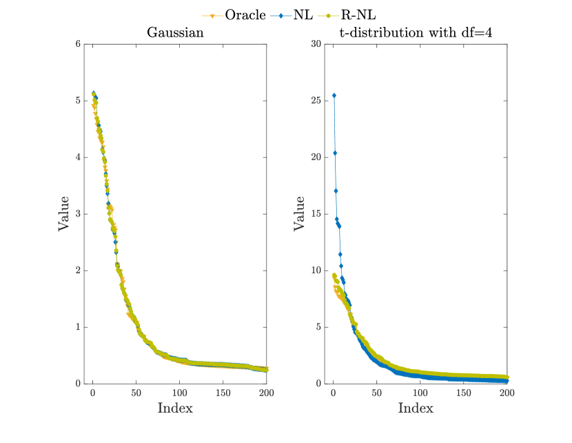
Figure 1: Comparison of the estimated values of nonlinear shrinkage and R-NL. The theoretical optimal eigenvalues $\mathbf{\hat{v}}_{j}^{\top}\boldsymbol{\Sigma}\mathbf{\hat{v}}_{j}$ are denoted by ‘Oracle”. In the left panel the sample is taken from a multivariate Gaussian distribution and in the right panel from a multivariate $t$-distribution with 4 degrees of freedom. For both distributions the $(i,j)$ element of $\mathbf{H}$ is $0.7^{\mid i-j\mid}$, as in Chen et al., (2011). The number of observations is $n=300$ and the dimension is $p=200$.

3 Methodology

We assume to observe an i.i.d. sample $\mathbb{Y}\mathrel{\vbox{\hbox{\scriptsize.}\hbox{\scriptsize.}}}=\{\mathbf{Y}_{1},\ldots,\mathbf{Y}_{n}\}$ from a $p$-dimensional elliptical distribution. If $\mathbf{Y}$ has an elliptical distribution it can be represented as

$$\mathbf{Y}\stackrel{{\scriptstyle D}}{{=}}\boldsymbol{\mu}+R\mathbf{H}^{1/2}\boldsymbol{\xi}~{},$$ (1)

where $R$ is a positive random variable, and $\boldsymbol{\xi}$ is uniformly distributed on the $p$-dimensional unit sphere, independently of $R$, and $\stackrel{{\scriptstyle D}}{{=}}$ denotes equality in distribution (Cambanis et al.,, 1981). The dispersion matrix $\mathbf{H}$ is assumed to be symmetric positive-definite (pd), with eigendecomposition $\mathbf{H}=\mathbf{V}\boldsymbol{\Lambda}\mathbf{V}^{\top}$. If $\mathbf{Y}$ meets (1), we write $\mathbf{Y}\sim E_{p}(\boldsymbol{\mu},\mathbf{H},g)$, where $g$ is the “generator” that identifies the distribution of $R$; for example, see Fang et al., (1990). We assume this generator to exist, which is equivalent to $R$ having a density (Fang et al.,, 1990).

In the following we restrict ourselves to distributions of the form (1) with $\boldsymbol{\mu}=\mathbf{0}$ and such that second moments exist. The assumption $\boldsymbol{\mu}=\mathbf{0}$ is used for simplicity, though it is not necessarily restrictive in the context of elliptical distributions. We refer to the discussion in (Goes et al.,, 2020, Section 2). Then $\operatorname*{Var}(\mathbf{Y})=c\mathbf{H}$ for some $c>0$. Following Chen et al., (2011), we will normalize our estimators of $\mathbf{H}$ to have trace $p$. We note however that, to obtain an estimator of $\boldsymbol{\Sigma}$, one could instead normalize the estimator to have the same trace as $\hat{\mathbf{S}}$. As an illustration, in the example from the right panel of Figure 1, $\operatorname{Tr}(\mathbf{\hat{S}})\approx 428$ whereas $\operatorname{Tr}(\boldsymbol{\Sigma})=400$.

3.1 Robust Nonlinear Shrinkage

We start by outlining our main idea. Let $\|\cdot\|$ be the Euclidean norm on ${\mathbb{R}}^{p}$. As shown in Tyler, 1987b , if $\mathbf{Y}\sim E_{p}(\boldsymbol{\mu},\mathbf{H},g)$, $\mathbf{Z}\mathrel{\vbox{\hbox{\scriptsize.}\hbox{\scriptsize.}}}=\frac{\mathbf{Y}}{\|\mathbf{Y}\|}$ has a central angular Gaussian distribution with density

$$p(\mathbf{z};\mathbf{H})\propto|\mathbf{H}|^{-1/2}\cdot\left(\mathbf{z}^{\top}\mathbf{H}^{-1}\mathbf{z}\right)^{-p/2}~{},$$ (2)

where for $a,b\in{\mathbb{R}}$, $a\propto b$ means there exists $c>0$ with $a=cb$. We will also write $\mathbf{A}\propto\mathbf{B}$, for two $p\times p$ matrices $\mathbf{A},\mathbf{B}$ if $\mathbf{A}=c\mathbf{B}$. The likelihood in (2) is the starting point of the original Tyler’s method. Taking the derivative of (2), Tyler’s estimator $\mathbf{\hat{H}}_{T}$ is implicitly given by the following condition:

$$\mathbf{\hat{H}}_{T}=\frac{p}{n}\sum_{t=1}^{n}\frac{\mathbf{Z}_{t}\mathbf{Z}_{t}^{\top}}{\mathbf{Z}_{t}^{\top}\mathbf{\hat{H}}_{T}^{-1}\mathbf{Z}_{t}}~{}.$$ (3)

This estimator is obtained as the limit of the iterations

$$\mathbf{\hat{H}}^{[\ell+1]}\ \propto\ \frac{p}{n}\sum_{t=1}^{n}\frac{\mathbf{Z}_{t}\mathbf{Z}_{t}^{\top}}{\mathbf{Z}_{t}^{\top}(\mathbf{\hat{H}}^{[\ell]})^{-1}\mathbf{Z}_{t}}~{},$$ (4)

where $\propto$ indicates that $\mathbf{\hat{H}}^{[\ell+1]}$ is actually obtained after an additional trace-normalization step; for example, see Tyler, 1987a or Chen et al., (2011). Robust linear shrinkage methods such as the method of Chen et al., (2011) augment (4) by shrinking towards the identity matrix in each iteration. That is, if for an $p\times p$ matrix $\mathbf{A}$ and $\rho\in[0,1]$, we define $\mbox{LS}\left(\mathbf{A},\rho\right)\mathrel{\vbox{\hbox{\scriptsize.}\hbox{\scriptsize.}}}=(1-\rho)\mathbf{A}+\rho\mathbf{I}$, then the robust linear shrinkage estimator is obtained from the iterations

$$\mathbf{\hat{H}}^{[\ell+1]}\ \propto\ \mbox{LS}\left(\frac{p}{n}\sum_{t=1}^{n}\frac{\mathbf{Z}_{t}\mathbf{Z}_{t}^{\top}}{\mathbf{Z}_{t}^{\top}(\mathbf{\hat{H}}^{[\ell]})^{-1}\mathbf{Z}_{t}},\rho\right)~{},$$ (5)

where again $\propto$ indicates a trace-normalization step.

Similarly, denote for any symmetric pd matrix $\mathbf{A}$ by $\mbox{NL}\left(\mathbf{A}\right)$ the matrix that is obtained when using nonlinear shrinkage on $\mathbf{A}$. A few clarifications are in order at this point. First, in the existing literature on nonlinear shrinkage, $\mathbf{A}$ is always the sample covariance matrix; but the ‘algorithm’ of nonlinear shrinkage allows for a more general input instead. Second, there are (at least) three different nonlinear shrinkage schemes by now: the numerical scheme called QuEST of Ledoit and Wolf, (2015), the analytical scheme of Ledoit and Wolf, (2020), and the QIS method of Ledoit and Wolf, 2022b , which is also of analytical nature; our methodology allows for the use of any such scheme, with our personal choice being the QIS method. Third, any ‘algorithm’ of nonlinear shrinkage needs as an additional input to $\mathbf{A}$, which of course determines the dimension $p$, also the sample size $n$, which we may treat as fixed and known in our methodology.

Applying nonlinear shrinkage to the matrix $\mathbf{A}$ leaves its eigenvectors unchanged and only changes its eigenvalues. The way the eigenvalues are changed depends on the particular nonlinear shrinkage scheme; for example, see (Ledoit and Wolf, 2022b, , Section 4.5) for the details concerning the QIS method. In analogy to the case of linear shrinkage, we could now apply nonlinear shrinkage each time in the above iteration. That is, we could iterate

$$\mathbf{\hat{H}}^{[\ell+1]}\ \propto\ \mbox{NL}\left(\frac{p}{n}\sum_{t=1}^{n}\frac{\mathbf{Z}_{t}\mathbf{Z}_{t}^{\top}}{\mathbf{Z}_{t}^{\top}(\mathbf{\hat{H}}^{[\ell]})^{-1}\mathbf{Z}_{t}}\right)~{},$$ (6)

where the input to NL corresponds to the sample covariance matrix of the scaled data $\mathbf{Z}_{t}/(\mathbf{Z}_{t}^{\top}(\mathbf{\hat{H}}^{[\ell]})^{-1}\mathbf{Z}_{t}/p)^{1/2}.$ Unfortunately, contrary to the case of linear shrinkage, it is not clear how to ensure convergence for such an approach. However, we note that iteration (6) can be seen as a simultaneous iteration over the eigenvalues and eigenvectors, whereby only the former is changed by nonlinear shrinkage. Following the ideas in Hediger and Näf, (2022), we instead aim to iterate over the eigenvectors for fixed (shrunken) eigenvalues. That is, after the first iteration, we fix the eigenvalues obtained by nonlinear shrinkage, denoted $\boldsymbol{\Lambda}_{0}$. Choosing $\mathbf{\hat{H}}^{[0]}=\mathbf{I}$, this corresponds to using nonlinear shrinkage on the sample covariance matrix of $\mathbb{Z}\mathrel{\vbox{\hbox{\scriptsize.}\hbox{\scriptsize.}}}=\{\mathbf{Z}_{1},\ldots,\mathbf{Z}_{T}\}$, with $\mathbf{Z}_{t}\mathrel{\vbox{\hbox{\scriptsize.}\hbox{\scriptsize.}}}=\mathbf{Y}_{t}/\|\mathbf{Y}_{t}\|$. It should be mentioned here that any nonlinear shrinkage scheme ensures that the elements on the diagonal of $\boldsymbol{\Lambda}_{0}$, denoted $\hat{\delta}_{j}$, $j=1,\ldots,p$, are all strictly positive.

We then optimize the likelihood of the central angular Gaussian distribution only with respect to the orthogonal matrix $\mathbf{V}$. That is, we solve,

$$\mathbf{\hat{V}} \mathrel{\vbox{\hbox{\scriptsize.}\hbox{\scriptsize.}}}=\operatorname*{arg\,max}_{\mathbf{U}\in\mathcal{O}}\sum_{t=1}^{n}\ln(p(\mathbf{Z}_{t};\mathbf{U},\boldsymbol{\Lambda}_{0}))$$

$$=\operatorname*{arg\,min}_{\mathbf{U}\in\mathcal{O}}\frac{1}{n}\sum_{t=1}^{n}\ln\left(\mathbf{Z}_{t}^{\top}\mathbf{U}\boldsymbol{\Lambda}_{0}^{-1}\mathbf{U}^{\top}\mathbf{Z}_{t}\right)~{},$$ (7)

where $\mathcal{O}\mathrel{\vbox{\hbox{\scriptsize.}\hbox{\scriptsize.}}}=\{\mathbf{U}:\mathbf{U}^{\top}\mathbf{U}=\mathbf{U}\mathbf{U}^{\top}=\mathbf{I}$} is the orthogonal group. Finally, once $\mathbf{\hat{V}}$ is obtained, $\boldsymbol{\Lambda}_{0}$ is updated. That is, we apply nonlinear shrinkage to the covariance matrix of the standardized data

$$\tilde{\mathbf{Z}}_{t}\mathrel{\vbox{\hbox{\scriptsize.}\hbox{\scriptsize.}}}=\frac{\mathbf{Z}_{t}}{\sqrt{\mathbf{Z}_{t}^{\top}\mathbf{\hat{V}}\boldsymbol{\Lambda}_{0}^{-1}\mathbf{\hat{V}}^{\top}\mathbf{Z}_{t}/p}}~{},t=1,\ldots,n,$$ (8)

to obtain $\boldsymbol{\Lambda}_{R}$. The final estimate is then given as

$$\mathbf{\hat{H}}\mathrel{\vbox{\hbox{\scriptsize.}\hbox{\scriptsize.}}}=p\cdot\mathbf{\hat{V}}\boldsymbol{\Lambda}_{R}\mathbf{\hat{V}}^{\top}/\operatorname{Tr}(\mathbf{\hat{V}}\boldsymbol{\Lambda}_{R}\mathbf{\hat{V}}^{\top})~{}.$$ (9)

Since, as we will show below, the eigenvectors of the sample covariance matrix of $\{\mathbf{\tilde{Z}}_{1},\ldots,\mathbf{\tilde{Z}}_{n}\}$ are again given by $\mathbf{\hat{V}}$, it holds that,

$$\mathbf{\hat{H}}\ \propto\ \mbox{NL}\left(\frac{1}{n}\sum_{t=1}^{n}\frac{\mathbf{Z}_{t}\mathbf{Z}_{t}^{\top}}{\mathbf{Z}_{t}^{\top}\mathbf{\hat{V}}\boldsymbol{\Lambda}_{0}^{-1}\mathbf{\hat{V}}^{\top}\mathbf{Z}_{t}}/p\right)~{}.$$

The whole procedure is summarized in Algorithm 2. We now detail how to solve (3.1).

For an $p\times p$ symmetric pd matrix $\mathbf{A}$, let

$$\mathbf{A}=\mathbf{U}_{A}\boldsymbol{\Lambda}_{A}\mathbf{U}_{A}^{\top}\ ,$$

be its eigendecomposition, where we assume the elements of $\boldsymbol{\Lambda}_{A}$ to be ordered from smallest to largest. We define $\mathcal{E}$ to be the operator that returns all possible matrices of eigenvectors. That is, $\mathcal{E}(\mathbf{A})$ is a subset of $\mathcal{O}$ and for any $\mathbf{U}\in\mathcal{E}(\mathbf{A})$, $\mathbf{U}^{\top}\mathbf{A}\mathbf{U}$ is a diagonal matrix with elements ordered from smallest to largest.

We also define in the following for $\mathbf{U}\in\mathcal{O}$,

$$F\left(\mathbf{U}\right)\mathrel{\vbox{\hbox{\scriptsize.}\hbox{\scriptsize.}}}=\sum_{t=1}^{n}\frac{\mathbf{Z}_{t}\mathbf{Z}_{t}^{\top}}{\mathbf{Z}_{t}^{\top}\mathbf{U}\boldsymbol{\Lambda}_{0}^{-1}\mathbf{U}^{\top}\mathbf{Z}_{t}}~{},$$ (10)

where the dependence on $\mathbf{Z}_{1},\dots,\mathbf{Z}_{n}$ and $\boldsymbol{\Lambda}_{0}$ is suppressed to keep notation compact.

lemmalone A minimizer $\mathbf{\hat{V}}$ of (3.1) exists and meets the condition

$$\mathbf{\hat{V}}^{\top}F\left(\mathbf{\hat{V}}\right)\mathbf{\hat{V}}\boldsymbol{\Lambda}_{0}^{-1}=\boldsymbol{\Lambda}_{0}^{-1}\mathbf{\hat{V}}^{\top}F\left(\mathbf{\hat{V}}\right)\mathbf{\hat{V}}~{}.$$ (11)

Proof

Since the orthogonal group is compact (Absil et al.,, 2007, Ch. 3) and

$$\mathbf{U}\mapsto f(\mathbf{U}):=\frac{1}{n}\sum_{t=1}^{n}\ln\left(\mathbf{Z}_{t}^{\top}\mathbf{U}\boldsymbol{\Lambda}_{0}^{-1}\mathbf{U}^{\top}\mathbf{Z}_{t}\right)~{},$$ (12)

is continuous, $f(\mathbf{U})$ takes its minimal and maximal value on $\mathcal{O}$. Thus there exists $\mathbf{\hat{V}}\in\mathcal{O}$ such that $\mathbf{\hat{V}}$ minimizes $f$.

On the other hand, according to Wen and Yin, (2013), if $\mathbf{\hat{V}}$ is a minimizer of $f$, it must satisfy the following first-order conditions:

$$G\mathbf{\hat{V}}^{\top}-\mathbf{\hat{V}}G^{\top}=\mathbf{0}~{},$$

where $G$ is the unconstrained gradient of problem (3.1),

$$G:=\frac{1}{n}\sum_{t=1}^{n}\frac{1}{\mathbf{Z}_{t}^{\top}\mathbf{\hat{V}}\boldsymbol{\Lambda}_{0}^{-1}\mathbf{\hat{V}}^{\top}\mathbf{Z}_{t}}\mathbf{Z}_{t}\mathbf{Z}_{t}^{\top}\mathbf{\hat{V}}\boldsymbol{\Lambda}_{0}^{-1}~{}.$$

Thus

$$\sum_{t=1}^{n}\left(\frac{\mathbf{Z}_{t}\mathbf{Z}_{t}^{\top}\mathbf{\hat{V}}\boldsymbol{\Lambda}_{0}^{-1}\mathbf{\hat{V}}^{\top}}{\mathbf{Z}_{t}^{\top}\mathbf{\hat{V}}\boldsymbol{\Lambda}_{0}^{-1}\mathbf{\hat{V}}^{\top}\mathbf{Z}_{t}}-\frac{\mathbf{\hat{V}}\boldsymbol{\Lambda}_{0}^{-1}\mathbf{\hat{V}}^{\top}\mathbf{Z}_{t}\mathbf{Z}_{t}^{\top}}{\mathbf{Z}_{t}^{\top}\mathbf{\hat{V}}\boldsymbol{\Lambda}_{0}^{-1}\mathbf{\hat{V}}^{\top}\mathbf{Z}_{t}}\right)=\mathbf{0}$$

$$\mathbf{\hat{V}}^{\top}\sum_{t=1}^{n}\frac{\mathbf{Z}_{t}\mathbf{Z}_{t}^{\top}}{\mathbf{Z}_{t}^{\top}\mathbf{\hat{V}}\boldsymbol{\Lambda}_{0}^{-1}\mathbf{\hat{V}}\boldsymbol{\Lambda}_{0}^{-1}\mathbf{Z}_{t}}\mathbf{\hat{V}}\boldsymbol{\Lambda}_{0}^{-1}$$

$$-\boldsymbol{\Lambda}_{0}^{-1}\mathbf{\hat{V}}^{\top}\sum_{t=1}^{n}\frac{\mathbf{Z}_{t}\mathbf{Z}_{t}^{\top}}{\mathbf{Z}_{t}^{\top}\mathbf{\hat{V}}\boldsymbol{\Lambda}_{0}^{-1}\mathbf{\hat{V}}^{\top}\mathbf{Z}_{t}}\mathbf{\hat{V}}=\mathbf{0}~{}.$$

Hence, any minimizer $\mathbf{\hat{V}}\in\mathcal{O}$ meets (11).
_■

The necessary condition in (11) is true in particular if $\mathbf{\hat{V}}$ diagonalizes $F\left(\mathbf{\hat{V}}\right)$, or

$$\mathbf{\hat{V}}\in\mathcal{E}\left(\frac{1}{n}\sum_{t=1}^{n}\frac{\mathbf{Z}_{t}\mathbf{Z}_{t}^{\top}}{\mathbf{Z}_{t}^{\top}\mathbf{\hat{V}}\boldsymbol{\Lambda}_{0}^{-1}\mathbf{\hat{V}}^{\top}\mathbf{Z}_{t}}\right)~{},$$ (13)

in analogy to (3). Thus given $\boldsymbol{\Lambda}_{0}$, we propose the following iterations

$$\mathbf{V}^{[\ell+1]} \in\mathcal{E}\left(\frac{1}{n}\sum_{t=1}^{n}\frac{\mathbf{Z}_{t}\mathbf{Z}_{t}^{\top}}{\mathbf{Z}_{t}^{\top}\mathbf{V}^{[\ell]}\boldsymbol{\Lambda}_{0}^{-1}(\mathbf{V}^{[\ell]})^{\top}\mathbf{Z}_{t}}\right)~{},$$ (14)

starting with

$$\mathbf{V}^{[1]}\in\mathcal{E}\left(\frac{1}{n}\sum_{t=1}^{n}\frac{\mathbf{Z}_{t}\mathbf{Z}_{t}^{\top}}{\|\mathbf{Z}_{t}\|}\right)=\mathcal{E}\left(\frac{1}{n}\sum_{t=1}^{n}\mathbf{Z}_{t}\mathbf{Z}_{t}^{\top}\right)~{}.$$ (15)

As noted above, this corresponds to the iterations in (Breloy et al.,, 2019, Algorithm 1), for $\alpha=\infty$. We also note that the time complexity in each iteration is the same as for the iterations of the original Tyler’s method in (4), namely $O(np^{2}+p^{3})$; for example, see Danon and Garber, (2022).

We now proceed by showing that any sequence generated by these iterations has a limit $\mathbf{V}^{[\infty]}$ such that (11) holds. To this end we adapt the approach taken in Wiesel, (2012); Razaviyayn et al., (2013); Sun et al., (2014) and define the surrogate function

$$g(\mathbf{U}\mid\mathbf{V}^{[\ell]})\mathrel{\vbox{\hbox{\scriptsize.}\hbox{\scriptsize.}}}= \frac{1}{n}\sum_{t=1}^{n}\ln\left(\mathbf{Z}_{t}^{\top}\mathbf{V}^{[\ell]}\boldsymbol{\Lambda}_{0}^{-1}(\mathbf{V}^{[\ell]})^{\top}\mathbf{Z}_{t}\right)$$

$$+\frac{1}{n}\sum_{t=1}^{n}\frac{\mathbf{Z}_{t}^{\top}\mathbf{U}\boldsymbol{\Lambda}_{0}^{-1}\mathbf{U}^{\top}\mathbf{Z}_{t}}{\mathbf{Z}_{t}^{\top}\mathbf{V}^{[\ell]}\boldsymbol{\Lambda}_{0}^{-1}(\mathbf{V}^{[\ell]})^{\top}\mathbf{Z}_{t}}-1~{}.$$ (16)

Then for $f(\mathbf{U})\mathrel{\vbox{\hbox{\scriptsize.}\hbox{\scriptsize.}}}=\frac{1}{n}\sum_{t=1}^{n}\ln\left(\mathbf{Z}_{t}^{\top}\mathbf{U}\boldsymbol{\Lambda}_{0}^{-1}\mathbf{U}^{\top}\mathbf{Z}_{t}\right)$,

lemmalthree The surrogate function $g$ satisfies:

$$f(\mathbf{U}) \leq g(\mathbf{U}\mid\mathbf{V}^{[\ell]})\text{ for all }\mathbf{U},\mathbf{V}^{[\ell]}\in\mathcal{O}$$ (17)

$$f(\mathbf{V}^{[\ell]}) =g(\mathbf{V}^{[\ell]}\mid\mathbf{V}^{[\ell]})~{},$$ (18)

and for $\mathbf{V}^{[\ell+1]}$ as in (14),

$$g(\mathbf{V}^{[\ell+1]}\mid\mathbf{V}^{[\ell]})\leq g(\mathbf{U}\mid\mathbf{V}^{[\ell]})\text{ for all }\mathbf{U}\in\mathcal{O}~{}.$$ (19)

Proof

The first inequality follows from the fact that, for any $a>0$, $\log(x)\leq\log(a)+(\frac{x}{a}-1)$ (Wiesel, (2012)), whereas the second equality is trivial. For the last claim, we can write

$$\operatorname*{arg\,min}_{\mathbf{U}\in\mathcal{O}}g(\mathbf{U}\mid\mathbf{V}^{[\ell]})$$

$$=\operatorname*{arg\,min}_{\mathbf{U}\in\mathcal{O}}\mbox{Tr}\left(\frac{1}{n}\sum_{t=1}^{n}\frac{\mathbf{Z}_{t}\mathbf{Z}_{t}^{\top}}{\mathbf{Z}_{t}^{\top}\mathbf{V}^{[\ell]}\boldsymbol{\Lambda}_{0}^{-1}(\mathbf{V}^{[\ell]})^{\top}\mathbf{Z}_{t}}\mathbf{U}\boldsymbol{\Lambda}_{0}^{-1}\mathbf{U}^{\top}\right)~{}.$$

Since we assume $\boldsymbol{\Lambda}_{0}$ has ordered values, this is globally minimized when $\mathbf{U}$ is chosen to diagonalize $\frac{1}{n}\sum_{t=1}^{n}\frac{\mathbf{Z}_{t}\mathbf{Z}_{t}^{\top}}{\mathbf{Z}_{t}^{\top}\mathbf{V}^{[\ell]}\boldsymbol{\Lambda}_{0}^{-1}(\mathbf{V}^{[\ell]})^{\top}\mathbf{Z}_{t}}$; for example, see Hediger and Näf, (2022).
_■

Define now the set of critical points as $\mathcal{V}\subset\mathcal{O}$, that is,

$$\mathcal{V}:=\{\mathbf{\hat{V}}\in\mathcal{O}\text{ such that }\eqref{critical_conditions}\text{ holds}\}~{},$$

and let for all $\mathbf{U}\in\mathcal{O}$,

$$d(\mathbf{U},\mathcal{V}):=\inf_{\mathbf{\hat{V}}\in\mathcal{V}}\|\mathbf{\hat{V}}-\mathbf{U}\|_{F}~{},$$

as in Razaviyayn et al., (2013). Using Lemma Proof the following convergence result can be obtained.

theoremthmone For any sequence $(\mathbf{V}^{[\ell]})_{\ell=1}^{\infty}$ generated by the above iterations,

$$f(\mathbf{V}^{[\ell+1]})\leq f(\mathbf{V}^{[\ell]})~{},\text{ for all }\ell,$$ (20)

and

$$\lim_{\ell\to\infty}d(\mathbf{V}^{[\ell]},\mathcal{V})=0~{}.$$ (21)

Proof

The proof closely follows the argument in (Razaviyayn et al.,, 2013, Theorem 1, Corollary 1). Using Lemma Proof, we have that for all $\ell$,

$$f(\mathbf{V}^{[\ell+1]})\leq g(\mathbf{V}^{[\ell+1]}\mid\mathbf{V}^{[\ell]})\leq g(\mathbf{V}^{[\ell]}\mid\mathbf{V}^{[\ell]})=f(\mathbf{V}^{[\ell]})~{},$$

proving the first part. For the second, since the orthogonal group $\mathcal{O}$ is compact, there exists a subsequence $(\mathbf{V}^{[\ell_{k}]})_{k=1}^{\infty}$ of $(\mathbf{V}^{[\ell]})_{\ell=1}^{\infty}$ that converges to $\mathbf{V}^{[\infty]}\in\mathcal{O}$. Additionally, for all $\mathbf{U}\in\mathcal{O}$,

$$g(\mathbf{U}\mid\mathbf{V}^{[\ell_{k}]})\geq g(\mathbf{V}^{[\ell_{k}+1]}\mid\mathbf{V}^{[\ell_{k}]})\geq f(\mathbf{V}^{[\ell_{k}+1]})$$

$$\geq f(\mathbf{V}^{[\ell_{k+1}]})=g(\mathbf{V}^{[\ell_{k+1}]}\mid\mathbf{V}^{[\ell_{k+1}]})~{},$$

since by the properties of subsequences $\ell_{k+1}\geq\ell_{k}+1$. Letting $k\to\infty$, thanks to the joint continuity of $(\mathbf{U}_{1},\mathbf{U}_{2})\mapsto g(\mathbf{U}_{1}\mid\mathbf{U}_{2})$, this implies

$$g(\mathbf{U}\mid\mathbf{V}^{[\infty]})\geq g(\mathbf{V}^{[\infty]}\mid\mathbf{V}^{[\infty]})~{},\text{for all }\mathbf{U}\in\mathcal{O}.$$

Thus $\mathbf{V}^{[\infty]}$ is the global minimizer of the function $\mathbf{U}\mapsto g(\mathbf{U}\mid\mathbf{V}^{[\infty]})$. In particular, the first-order conditions must hold: Thus

$$G(\mathbf{V}^{[\infty]})^{\top}-\mathbf{V}^{[\infty]}G^{\top}=\mathbf{0}~{},$$

where $G$ is the unconstrained derivative at $\mathbf{V}^{[\infty]}$:

$$G:=\frac{1}{n}\sum_{t=1}^{n}\frac{1}{\mathbf{Z}_{t}^{\top}\mathbf{V}^{[\infty]}\boldsymbol{\Lambda}_{0}^{-1}(\mathbf{V}^{[\infty]})^{\top}\mathbf{Z}_{t}}\mathbf{Z}_{t}\mathbf{Z}_{t}^{\top}\mathbf{V}^{[\infty]}\boldsymbol{\Lambda}_{0}^{-1}~{}.$$

Thus it holds that

$$(\mathbf{V}^{[\infty]})^{\top}\sum_{t=1}^{n}\frac{\mathbf{Z}_{t}\mathbf{Z}_{t}^{\top}}{\mathbf{Z}_{t}^{\top}(\mathbf{V}^{[\infty]})^{\top}\boldsymbol{\Lambda}_{0}^{-1}\mathbf{V}^{[\infty]}\boldsymbol{\Lambda}_{0}^{-1}\mathbf{Z}_{t}}\mathbf{V}^{[\infty]}\boldsymbol{\Lambda}_{0}^{-1}$$

$$-\boldsymbol{\Lambda}_{0}^{-1}(\mathbf{V}^{[\infty]})^{\top}\sum_{t=1}^{n}\frac{\mathbf{Z}_{t}\mathbf{Z}_{t}^{\top}}{\mathbf{Z}_{t}^{\top}\mathbf{V}^{[\infty]}\boldsymbol{\Lambda}_{0}^{-1}(\mathbf{V}^{[\infty]})^{\top}\mathbf{Z}_{t}}\mathbf{V}^{[\infty]}=\mathbf{0}~{},$$

which corresponds to the desired first-order conditions for the minimization of $f$ and thus $\mathbf{V}^{[\infty]}\in\mathcal{V}$, or $d(\mathbf{V}^{[\infty]},\mathcal{V})=0$.

Repeating this argument, it follows that any subsequence of $(\mathbf{V}^{[\ell]})_{\ell=1}^{\infty}$ has a further subsequence converging to some $\mathbf{V}^{[\infty]}$ (depending on the subsequence) with $d(\mathbf{V}^{[\infty]},\mathcal{V})=0$. Now assume the overall sequence does not converge to a point in $\mathcal{V}$. Then there is a subsequence $(\mathbf{V}^{[\ell_{k}]})_{k=1}^{\infty}$ such that for all $k$

$$d(\mathbf{V}^{[\ell_{k}]},\mathcal{V})\geq\varepsilon~{},$$

for some $\varepsilon>0$. But then this would be true also for any subsequence, a contradiction.
_■

Thus, as $\ell\to\infty$, $\mathbf{V}^{[\ell]}$ gets arbitrary close to a critical point. This leads to the following convergence criterion:

$$\|(\mathbf{V}^{[\ell-1]})^{\top}F\left(\mathbf{V}^{[\ell-1]}\right)\mathbf{V}^{[\ell-1]}\boldsymbol{\Lambda}_{0}^{-1}$$

$$-\boldsymbol{\Lambda}_{0}^{-1}(\mathbf{V}^{[\ell]})^{\top}F\left(\mathbf{V}^{[\ell]}\right)\mathbf{V}^{[\ell]}\|_{F}\leq\epsilon~{},$$

where $\epsilon>0$ is some convergence tolerance. This criterion is used in Algorithm 1 and we set $\epsilon=10^{-10}$ in Sections 4 and 5.

Although R-NL is no longer in the same class of estimators as nonlinear shrinkage, namely the class of Stein, (1975, 1986), an interesting question is whether it is still rotation-equivariant. An estimator $\mathbf{\hat{H}}$ applied to $\mathbb{Y}=\{\mathbf{Y}_{1},\ldots,\mathbf{Y}_{T}\}$ is rotation-equivariant if, for any rotation $\mathbf{R}$ and rotated data $\mathbf{\bar{Y}}_{t}\mathrel{\vbox{\hbox{\scriptsize.}\hbox{\scriptsize.}}}=\mathbf{R}\mathbf{Y}_{t}$, $t=1,\ldots,n$, the estimate of the rotated data, $\mathbf{\hat{H}}_{\mathbf{R}}$, satisfies

$$\mathbf{\hat{H}}_{\mathbf{R}}=\mathbf{R}\mathbf{\hat{H}}\mathbf{R}^{\top}~{}.$$ (22)

This is true for any estimator in the class of Stein, (1975, 1986) and, therefore, in particular for nonlinear shrinkage. We now show that this is true for R-NL as well, using the following lemma:

lemmalfour Let $\mathbf{R}$ be an arbitrary rotation, $\mathbf{\bar{Z}}_{t}\mathrel{\vbox{\hbox{\scriptsize.}\hbox{\scriptsize.}}}=\mathbf{R}\mathbf{Z}_{t}$ and $\mathbf{V}^{[\ell]}_{r}$ be the $\ell$th iteration of Algorithm 1 applied to $\{\mathbf{\bar{Z}}_{1},\ldots,\mathbf{\bar{Z}}_{T}\}$. Then

$$\mathcal{E}\left(\frac{1}{n}\sum_{t=1}^{n}\frac{\mathbf{\bar{Z}}_{t}\mathbf{\bar{Z}}_{t}^{\top}}{\mathbf{\bar{Z}}_{t}^{\top}\mathbf{V}^{[\ell]}_{r}\boldsymbol{\Lambda}_{0}^{-1}(\mathbf{V}^{[\ell]}_{r})^{\top}\mathbf{\bar{Z}}_{t}}\right)=\left\{\mathbf{R}\mathbf{V}^{[\ell+1]}:\right.$$

$$\left.\mathbf{V}^{[\ell+1]}\in\mathcal{E}\left(\frac{1}{n}\sum_{t=1}^{n}\frac{\mathbf{Z}_{t}\mathbf{Z}_{t}^{\top}}{\mathbf{Z}_{t}^{\top}\mathbf{V}^{[\ell]}\boldsymbol{\Lambda}_{0}^{-1}(\mathbf{V}^{[\ell]})^{\top}\mathbf{Z}_{t}}\right)\right\}~{}.$$ (23)

Proof

It clearly holds that (23) is true for $\ell=0$. Assume (23) holds for $\ell$, we show that it holds for $\ell+1$: By assumption we can write $\mathbf{V}^{[\ell]}_{r}=\mathbf{R}\mathbf{V}^{[\ell]}$. Thus

$$\mathcal{E}\left(\frac{1}{n}\sum_{t=1}^{n}\frac{\mathbf{\bar{Z}}_{t}\mathbf{\bar{Z}}_{t}^{\top}}{\mathbf{\bar{Z}}_{t}^{\top}\mathbf{V}^{[\ell]}_{r}\boldsymbol{\Lambda}_{0}^{-1}(\mathbf{V}^{[\ell]}_{r})^{\top}\mathbf{\bar{Z}}_{t}}\right)$$

$$=\mathcal{E}\left(\mathbf{R}\frac{1}{n}\sum_{t=1}^{n}\frac{\mathbf{Z}_{t}\mathbf{Z}_{t}^{\top}}{\mathbf{Z}_{t}^{\top}\mathbf{V}^{[\ell]}\boldsymbol{\Lambda}_{0}^{-1}(\mathbf{V}^{[\ell]})^{\top}\mathbf{Z}_{t}}\mathbf{R}^{\top}\right)$$

$$=\mathbf{R}\mathcal{E}\left(\frac{1}{n}\sum_{t=1}^{n}\frac{\mathbf{Z}_{t}\mathbf{Z}_{t}^{\top}}{\mathbf{Z}_{t}^{\top}\mathbf{V}^{[\ell]}\boldsymbol{\Lambda}_{0}^{-1}(\mathbf{V}^{[\ell]})^{\top}\mathbf{Z}_{t}}\right)~{},$$

and thus (23) hold true.
_■

We note that the rotation of the original data in $\mathbb{Y}$ corresponds to a rotation of $\mathbb{Z}$, since for all $t$, $\mathbf{R}\mathbf{Y}_{t}/\|\mathbf{R}\mathbf{Y}_{t}\|=\mathbf{R}\mathbf{Y}_{t}/\|\mathbf{Y}_{t}\|=\mathbf{R}\mathbf{Z}_{t}$. Thus if $(\mathbf{V}^{[\ell]})_{\ell=1}^{\infty}$ is a sequence generated by Algorithm 1 for the data $\{\mathbf{Y}_{1},\ldots,\mathbf{Y}_{T}\}$, then $(\mathbf{R}\mathbf{V}^{[\ell]})_{\ell=1}^{\infty}$ is a sequence generated for the rotated data. Consequently, the corresponding estimate of $\mathbf{H}_{\mathbf{R}}$ for the rotated data will be of the form (22).

3.2 Uniqueness

The matrix $\mathbf{\hat{V}}$ in (13) (and consequently in (11)) is not unique in general. However, we are ultimately not interested in $\mathbf{\hat{V}}$, but in $\mathbf{\hat{V}}\boldsymbol{\Lambda}_{0}\mathbf{\hat{V}}^{\top}$. A natural question is thus whether $\mathbf{\hat{V}}\boldsymbol{\Lambda}_{0}\mathbf{\hat{V}}^{\top}$ is unique even if $\mathbf{\hat{V}}$ is not. This turns out to be true with probability one, as we detail now. Let in the following $\boldsymbol{\hat{\Lambda}}$ be the diagonal matrix of (ordered) eigenvalues of $F\bigl{(}\mathbf{\hat{V}}\bigr{)}$. It has the form $\boldsymbol{\hat{\Lambda}}=\boldsymbol{\hat{\Lambda}}_{+}$, if $p<n$ and

$$\boldsymbol{\hat{\Lambda}}=\begin{pmatrix}\mathbf{0}_{p-n+1,p-n+1}&\mathbf{0}_{p-n+1,n-1}\\ \mathbf{0}_{n-1,p-n+1}&\boldsymbol{\hat{\Lambda}}_{+}\end{pmatrix}, \text{ if }p\geq n~{},$$

where $\boldsymbol{\hat{\Lambda}}_{+}$ is a diagonal matrix with the largest $\min(n-1,p)$ eigenvalues and $\mathbf{0}_{n,p}$ is an $n\times p$ matrix of zeros. We denote the diagonal elements of $\boldsymbol{\hat{\Lambda}}$ as $\hat{\lambda}_{1},\ldots\hat{\lambda}_{p}$. Define similarly the matrix of eigenvalues of $F\left(\mathbf{V}^{[\ell-1]}\right)$ as $\boldsymbol{\hat{\Lambda}}^{[\ell]}$, with elements $\hat{\lambda}_{1}^{[\ell]},\ldots\hat{\lambda}_{p}^{[\ell]}$, and $\boldsymbol{\hat{\Lambda}}_{+}^{[\ell]}$ as the largest $\min(n-1,p)$ eigenvalues of $\boldsymbol{\hat{\Lambda}}^{[\ell]}$.

lemmaltwo Assume that whenever $\hat{\lambda}_{i}=\hat{\lambda}_{j}$, also $\hat{\delta}_{i}=\hat{\delta}_{j}$, for $j,i\in\{1,\ldots,p\}$. Then if $\mathbf{\hat{V}}_{1}$ and $\mathbf{\hat{V}}_{2}$ meet (13),

$$\mathbf{\hat{V}}_{1}\boldsymbol{\Lambda}_{0}(\mathbf{\hat{V}}_{1})^{\top}=\mathbf{\hat{V}}_{2}\boldsymbol{\Lambda}_{0}(\mathbf{\hat{V}}_{2})^{\top}.$$

Proof

If $\hat{\lambda}_{i}$ is unique, the corresponding eigenvector $\mathbf{v}_{i}$ is the basis of the one-dimensional space $\{\mathbf{u}:(F(\mathbf{\hat{V}})-\hat{\lambda}_{i}\mathbf{I})\mathbf{u}=\mathbf{0}\}$. As such if $\mathbf{v}_{i}^{1}$, $\mathbf{v}_{i}^{2}$ are the $i$th column of $\mathbf{\hat{V}}_{1}$ and $\mathbf{\hat{V}}_{2}$ respectively, it must hold that $\mathbf{v}_{i}^{1}=\mathbf{v}_{i}^{2}$ or $\mathbf{v}_{i}^{1}=-\mathbf{v}_{i}^{2}$. However as $\mathbf{\hat{V}}_{1}\boldsymbol{\Lambda}_{0}\mathbf{\hat{V}}_{1}^{\top}=\sum_{i=1}^{p}\hat{\delta}_{i}\mathbf{v}_{i}^{1}(\mathbf{v}_{i}^{1})^{\top}$ this does not affect the overall matrix. This holds true whether or not $\hat{\delta}_{i}$ in $\boldsymbol{\Lambda}_{0}$ is unique.

Now assume there is $\hat{\lambda}_{i}$ with multiplicity $p_{0}$, whereas all other $\hat{\lambda}_{j}$ are unique. By assumption, $\boldsymbol{\Lambda}_{0}$ mimics this pattern and we can reorder their values such that:

$$\boldsymbol{\hat{\Lambda}}=\begin{pmatrix}\boldsymbol{\hat{\Lambda}}_{1}&\mathbf{0}_{p-p_{0},p_{0}}\\ \mathbf{0}_{p_{0},p-p_{0}}&\boldsymbol{\hat{\Lambda}}_{2}\end{pmatrix}\text{ and }\boldsymbol{\Lambda}_{0}=\begin{pmatrix}\boldsymbol{\Lambda}_{0}^{1}&\mathbf{0}_{p-p_{0},p_{0}}\\ \mathbf{0}_{p_{0},p-p_{0}}&\boldsymbol{\Lambda}_{0}^{2}\end{pmatrix}~{},$$

where $\boldsymbol{\hat{\Lambda}}_{1}$ contains unique ordered values and $\boldsymbol{\hat{\Lambda}}_{2}$ of size $p_{0}\times p_{0}$ contains one value with multiplicity. By assumption, $\boldsymbol{\Lambda}_{0}^{1}$ might have values with multiplicity larger one, but $\boldsymbol{\Lambda}_{0}^{2}$ also contains only copies of one value. We similarly decompose the newly ordered $\mathbf{\hat{V}}_{1},\mathbf{\hat{V}}_{2}$:

$$\mathbf{\hat{V}}_{1}=[\mathbf{\hat{V}}_{11},\mathbf{\hat{V}}_{12}]\text{ and }\mathbf{\hat{V}}_{2}=[\mathbf{\hat{V}}_{21},\mathbf{\hat{V}}_{22}]~{}.$$

The columns of $\mathbf{\hat{V}}_{12},\mathbf{\hat{V}}_{22}$ now form an orthogonal basis of the $p_{0}$-dimensional eigenvectorspace. As such, we can express each column of $\mathbf{\hat{V}}_{12}$ as a linear combination of columns in $\mathbf{\hat{V}}_{22}$, that is there exists $\mathbf{A}\in{\mathbb{R}}^{p_{0}\times p_{0}}$, such that $\mathbf{\hat{V}}_{12}=\mathbf{\hat{V}}_{22}\mathbf{A}$. Moreover

$$\mathbf{I}=\mathbf{\hat{V}}_{12}^{\top}\mathbf{\hat{V}}_{12}=\mathbf{A}^{\top}\mathbf{\hat{V}}_{22}^{\top}\mathbf{\hat{V}}_{22}\mathbf{A}=\mathbf{A}^{\top}\mathbf{A}~{}.$$

Thus the columns of $\mathbf{A}$ are orthogonal and since it is square, it has full rank and $\mathbf{A}\mathbf{A}^{\top}=\mathbf{I}$ holds as well. Finally,

$$\mathbf{\hat{V}}_{1}\boldsymbol{\Lambda}_{0}\mathbf{\hat{V}}_{1}^{\top} =\mathbf{\hat{V}}_{11}\boldsymbol{\Lambda}_{0}^{1}\mathbf{\hat{V}}_{11}^{\top}+\mathbf{\hat{V}}_{12}\boldsymbol{\Lambda}_{0}^{2}\mathbf{\hat{V}}_{12}^{\top}$$

$$=\mathbf{\hat{V}}_{21}\boldsymbol{\Lambda}_{0}^{1}\mathbf{\hat{V}}_{21}^{\top}+\hat{\delta}_{i}\mathbf{\hat{V}}_{12}\mathbf{\hat{V}}_{12}^{\top}$$

$$=\mathbf{\hat{V}}_{21}\boldsymbol{\Lambda}_{0}^{1}\mathbf{\hat{V}}_{21}^{\top}+\hat{\delta}_{i}\mathbf{\hat{V}}_{22}\mathbf{A}\mathbf{A}^{\top}\mathbf{\hat{V}}_{22}^{\top}$$

$$=\mathbf{\hat{V}}_{2}\boldsymbol{\Lambda}_{0}\mathbf{\hat{V}}_{2}^{\top}~{}.$$

A similar approach can be used to show that the equality holds if several $\hat{\lambda}_{i}$ have multiplicity larger than one.
_■

Thus if the multiplicity of eigenvalues of $\boldsymbol{\hat{\Lambda}}$ implies the multiplicity of the corresponding eigenvalue in $\boldsymbol{\Lambda}_{0}$, the resulting matrix will also be the same. This is true in particular if $\hat{\lambda}_{i}\neq\hat{\lambda}_{j}$ for all $i,j$. Consequently, under the conditions of Lemma 3.2, $\mathbf{\hat{V}}$ in (13) is unique under the equivalence relation $\sim_{\boldsymbol{\Lambda}_{0}}$ with

$$\mathbf{U}_{1}\sim_{\boldsymbol{\Lambda}_{0}}\mathbf{U}_{2}\iff\mathbf{U}_{1}\boldsymbol{\Lambda}_{0}(\mathbf{U}_{1})^{\top}=\mathbf{U}_{2}\boldsymbol{\Lambda}_{0}(\mathbf{U}_{2})^{\top}.$$

More generally if we consider the space of equivalence classes $\mathcal{O}_{0}:=\mathcal{O}\setminus\sim_{\boldsymbol{\Lambda}_{0}}$ and define the metric

$$\tilde{d}_{\boldsymbol{\Lambda}_{0}}([\mathbf{U}_{1}],[\mathbf{U}_{2}]):=\|\mathbf{U}_{1}\boldsymbol{\Lambda}_{0}\mathbf{U}_{1}^{\top}-\mathbf{U}_{2}\boldsymbol{\Lambda}_{0}\mathbf{U}_{2}^{\top}\|_{F},$$

where $[\mathbf{U}]:=\{\mathbf{U}_{0}\in\mathcal{O}:\mathbf{U}_{0}\sim_{\boldsymbol{\Lambda}_{0}}\mathbf{U}\}$, we obtain the following lemma.

lemmalfive Assume that

$$\forall\ell\ \ \hat{\lambda}_{i}^{[\ell]}=\hat{\lambda}_{j}^{[\ell]}\implies\hat{\delta}_{i}=\hat{\delta}_{j}.$$ (24)

Then we can write iteration (14) in terms of equivalence classes:

$$[\mathbf{V}^{[\ell+1]}]=\mathcal{E}(F([\mathbf{V}^{[\ell]}]))~{}.$$ (25)

Moreover there exists $[\mathbf{\hat{V}}]\in\mathcal{O}_{0}$ such that (13) holds and the generated sequence $\left([\mathbf{V}^{[\ell]}]\right)_{\ell=1}^{\infty}$ satisfies

$$\tilde{d}_{\boldsymbol{\Lambda}_{0}}([\mathbf{V}^{[\ell]}],[\mathbf{\hat{V}}])\to 0~{}.$$

Proof

First we note that, since the values in $\boldsymbol{\Lambda}_{0}$ are all strictly larger than zero,

$$\mathbf{U}_{1}\sim_{\boldsymbol{\Lambda}_{0}}\mathbf{U}_{2}\iff\mathbf{U}_{1}\boldsymbol{\Lambda}_{0}^{-1}(\mathbf{U}_{1})^{\top}=\mathbf{U}_{2}\boldsymbol{\Lambda}_{0}^{-1}(\mathbf{U}_{2})^{\top}.$$

Thus for any two $\mathbf{U}_{1}\in[\mathbf{U}]$, $\mathbf{U}_{2}\in[\mathbf{U}]$, $F(\mathbf{U}_{1})=F(\mathbf{U}_{2})$, such that we may write $F$ directly as a function of the equivalence class, $F([\mathbf{U}])$. Moreover, since the eigenvalues of $F([\mathbf{V}]^{[\ell]})$ meet the multiplicity condition, the same proof as in Lemma 3.2 gives that any $\mathbf{U}_{1}\in\mathcal{E}(F(\mathbf{V}^{[\ell]}))$, $\mathbf{U}_{2}\in\mathcal{E}(F(\mathbf{V}^{[\ell]}))$ have $\mathbf{U}_{1}\sim_{\boldsymbol{\Lambda}_{0}}\mathbf{U}_{2}$. Thus (25) holds and we can write $[\mathbf{V}]^{[\ell]}=[\mathbf{V}^{[\ell]}]$.

Moreover, by the same argument as above, the function value $f(\mathbf{U})$ of any member of an equivalence class is the same, such that we may again write $f([\mathbf{U}])$. Finally $\mathcal{O}_{0}$ is still compact with the metric $\tilde{d}_{\boldsymbol{\Lambda}_{0}}$. Indeed consider a sequence $([\mathbf{U}_{n}])_{n}$ in $\mathcal{O}_{0}$. For each $n$ we choose an arbtriary representative $\mathbf{U}_{n}\in\mathcal{O}$, to form the sequence $\left(\mathbf{U}_{n}\right)_{n}$. Since $\mathcal{O}$ is compact, this sequence will have a convergent subsequence $\left(\mathbf{U}_{n_{k}}\right)_{k}$. We now show that the corresponding subsequence in $\mathcal{O}$, $\left([\mathbf{U}]_{n_{k}}\right)_{k}$ converges in $\mathcal{O}_{0}$. Indeed notice that for any convergent sequence, that is, $\left(\mathbf{U}_{n}\right)_{n}$ such that $\mathbf{U}_{n}\to\mathbf{U}$, it follows by the continuity of the matrix product that

$$\mathbf{U}_{n}\boldsymbol{\Lambda}_{0}\mathbf{U}_{n}^{\top}\to\mathbf{U}\boldsymbol{\Lambda}_{0}\mathbf{U}^{\top}~{},$$

or

$$\tilde{d}_{\boldsymbol{\Lambda}_{0}}([\mathbf{U}_{n}],[\mathbf{U}])=\|\mathbf{U}_{n}\boldsymbol{\Lambda}_{0}\mathbf{U}_{n}^{\top}\to\mathbf{U}\boldsymbol{\Lambda}_{0}\mathbf{U}^{\top}\|_{F}\to 0~{}.$$

Applying this to $\left([\mathbf{U}]_{n_{k}}\right)_{k}$, $\tilde{d}_{\boldsymbol{\Lambda}_{0}}([\mathbf{U}_{n_{k}}],[\mathbf{U}])\to 0$. Since the sequence was arbitrary, every sequence in $\mathcal{O}_{0}$ has a convergent subsequence in $\mathcal{O}_{0}$ and thus $(\mathcal{O}_{0},\tilde{d}_{\boldsymbol{\Lambda}_{0}})$ is compact.

Finally we can trace the same steps as in Theorem Proof to show that

$$\inf_{[\mathbf{\hat{V}}]\in\mathcal{V}_{0}}\tilde{d}_{\boldsymbol{\Lambda}_{0}}([\mathbf{V}^{[\ell]}],[\mathbf{\hat{V}}])\to 0~{},$$

where now the set $\mathcal{V}_{0}\subset\mathcal{O}_{0}$ such that (13) holds has only one member $[\mathbf{\hat{V}}]$.
_■

At first, it might seem unclear how to enforce the eigenvalue condition in Lemma Proof. However, since $\hat{\lambda}_{i}^{[\ell]}$, $i=1,\ldots,p$ are eigenvalues of the sample covariance matrix of the standardized sample, Theorem 1 of Okamoto, (1973) applies. This implies that the eigenvalues of $\boldsymbol{\hat{\Lambda}}_{+}^{[\ell]}$ are all nonzero and distinct with probability one. Thus we only need to ensure that, for $p\geq n$, the smallest $p-n+1$ eigenvalues in $\boldsymbol{\Lambda}_{0}$ are all the same. This is enforced in Algorithm 1 by simply setting the smallest $p-n+1$ values of $\boldsymbol{\Lambda}_{0}$ to the value with the highest multiplicity. The following lemma now obtains.

lemmanone Condition (24) holds with probability one.

We thus obtain uniqueness of $\mathbf{\hat{V}}\boldsymbol{\Lambda}_{0}\mathbf{\hat{V}}^{\top}$ and of $\mathbf{\hat{H}}$, up to scaling.

Inputs: centered data $\mathbb{Z}$, eigenvalue matrix $\boldsymbol{\Lambda}_{0}$;

Output: $\mathbf{\hat{V}}$;

Hyper-parameters: Convergence Tolerance $\epsilon$ ;

Initiate $\ell=0$, $c(0)=-\infty$, $c(1)=0$, $\mathbf{V}^{[0]}=\mathbf{I}$;

while $c(\ell+1)-c(\ell)>\epsilon$ do

       - Calculate $F\left(\mathbf{V}^{[\ell]}\right)$ as in (10) and its eigendecomposition $\mathbf{U}\boldsymbol{\hat{\Lambda}}^{[\ell+1]}\mathbf{U}^{\top}$, with $\boldsymbol{\hat{\Lambda}}^{[\ell+1]}$ ordered;

       - Take $\mathbf{V}^{[\ell+1]}=\mathbf{U}$;

       - $\ell=\ell+1$;

       - $c(\ell+1)=\|(\mathbf{V}^{[\ell-1]})^{\top}F\left(\mathbf{V}^{[\ell-1]}\right)\mathbf{V}^{[\ell-1]}\boldsymbol{\Lambda}_{0}^{-1}-\boldsymbol{\Lambda}_{0}^{-1}(\mathbf{V}^{[\ell]})^{\top}F\left(\mathbf{V}^{[\ell]}\right)\mathbf{V}^{[\ell]}\|_{F}$;

      

return $\mathbf{\hat{V}}=\mathbf{V}^{[\ell]}$

Algorithm 1 VIteration($\mathbb{Z}$, $\boldsymbol{\Lambda}_{0}$)

Inputs: centered data $\mathbb{Y}$;

Output: $\mathbf{\hat{H}}$;

- Calculate $\mathbb{Z}\mathrel{\vbox{\hbox{\scriptsize.}\hbox{\scriptsize.}}}=\{\mathbf{Z}_{1},\ldots\mathbf{Z}_{T}\}$ with $\mathbf{Z}_{t}\mathrel{\vbox{\hbox{\scriptsize.}\hbox{\scriptsize.}}}=\mathbf{Y}_{t}/\|\mathbf{Y}_{t}\|$, $t=1,\ldots,n$;

- Obtain the sorted eigenvalues $\boldsymbol{\Lambda}_{0}$ by applying NL to $\mathbb{Z}$;

- If $p\geq n$: Ensure that the last $p-n+1$ elements of $\boldsymbol{\Lambda}_{0}$ are equal;

- Obtain $\mathbf{\hat{V}}\mathrel{\vbox{\hbox{\scriptsize.}\hbox{\scriptsize.}}}=$ VIteration($\mathbb{Z},\boldsymbol{\Lambda}_{0}$) using Algorithm 1;

- Calculate $\tilde{\mathbf{Z}}_{t}$, $t=1,\ldots,n$, as in (8);

- Apply NL to the sample $\tilde{\mathbf{Z}}_{1},\ldots\tilde{\mathbf{Z}}_{n}$ to obtain $\boldsymbol{\Lambda}_{R}$;

- Calculate $\mathbf{\hat{H}}$ as in (9);

return $\mathbf{\hat{H}}$

Algorithm 2 R-NL($\mathbb{Y}$)

Inputs: centered data $\mathbb{Y}$;

Output: $\mathbf{\hat{H}}$;

- Calculate the diagonal matrix of sample standard deviations $\boldsymbol{\hat{\sigma}}$ of $\mathbb{Y}$;

- Calculate $\mathbb{X}\mathrel{\vbox{\hbox{\scriptsize.}\hbox{\scriptsize.}}}=\{\mathbf{X}_{1},\ldots,\mathbf{X}_{T}\}$ as in (26);

- Obtain $\mathbf{\hat{H}}_{0}\mathrel{\vbox{\hbox{\scriptsize.}\hbox{\scriptsize.}}}=$ R-NL($\mathbb{X}$) using Algorithm 2;

- Calculate $\mathbf{\hat{H}}\mathrel{\vbox{\hbox{\scriptsize.}\hbox{\scriptsize.}}}=p\cdot\boldsymbol{\hat{\sigma}}\mathbf{\hat{H}}_{0}\boldsymbol{\hat{\sigma}}/\operatorname{Tr}(\boldsymbol{\hat{\sigma}}\mathbf{\hat{H}}_{0}\boldsymbol{\hat{\sigma}})$;

return $\mathbf{\hat{H}}$

Algorithm 3 R-C-NL($\mathbb{Y}$)

3.3 Robust Correlation-Based Nonlinear Shrinkage

In the context of covariance matrix estimation, an alternative approach is to use shrinkage estimation for the correlation matrix and to estimate the vector of variances separately, after which one combines the two estimators to obtain a ‘final’ estimator of the covariance matrix itself. Such an approach is used by Hediger and Näf, (2022) in a static setting (that is, for i.i.d. data) and by Engle et al., (2019); De Nard et al., (2022) in a dynamic setting (that is, for time series data). It turns out that by adapting this approach for our method, a considerable boost in performance can be achieved in some settings.

In particular, we first calculate the sample variances $\hat{\sigma}_{1}^{2},\ldots,\hat{\sigma}_{p}^{2}$ and obtain the scaled data as

$$\mathbf{X}_{t}\mathrel{\vbox{\hbox{\scriptsize.}\hbox{\scriptsize.}}}=\boldsymbol{\hat{\sigma}}^{-1}\mathbf{Y}_{t}~{},$$ (26)

where $\boldsymbol{\hat{\sigma}}\mathrel{\vbox{\hbox{\scriptsize.}\hbox{\scriptsize.}}}=\mbox{diag}(\hat{\sigma}_{1},\ldots,\hat{\sigma}_{p})$. Then R-NL is applied to $\mathbf{Z}_{t}\mathrel{\vbox{\hbox{\scriptsize.}\hbox{\scriptsize.}}}=\boldsymbol{\hat{\sigma}}^{-1}\mathbf{Y}_{t}/\|\boldsymbol{\hat{\sigma}}^{-1}\mathbf{Y}_{t}\|$ to obtain $\hat{\mathbf{H}}_{0}\mathrel{\vbox{\hbox{\scriptsize.}\hbox{\scriptsize.}}}=p\mathbf{\hat{V}}\boldsymbol{\Lambda}_{R}\mathbf{\hat{V}}^{\top}/\operatorname{Tr}(\boldsymbol{\Lambda}_{R})$. From these two inputs, we calculate the ‘final’ estimator of $\mathbf{H}$ as

$$\mathbf{\hat{H}}\mathrel{\vbox{\hbox{\scriptsize.}\hbox{\scriptsize.}}}=p\cdot\boldsymbol{\hat{\sigma}}\hat{\mathbf{H}}_{0}\boldsymbol{\hat{\sigma}}/\operatorname{Tr}(\boldsymbol{\hat{\sigma}}\hat{\mathbf{H}}_{0}\boldsymbol{\hat{\sigma}})~{}.$$ (27)

The approach is called “R-C-NL” and is summarized in Algorithm 3.

As we demonstrate in Section 4 this ‘variation’ on our methodology can have a substantial (beneficial) effect on the performance of the estimator. However, a potential disadvantage of this approach is that R-C-NL is no longer rotation-equivariant.

4 Simulation Study

We compare our proposed two methods to several competitors in various simulation scenarios. From the collection of approaches that use Tyler’s method together with (linear) shrinkage, we tried to pick the ones most appropriate for our analysis, without handpicking them to showcase the performance of our method. In particular, we did not pick methods that require the choice of a tuning parameter (such as Sun et al., (2014); Yu et al., (2017); Yi and Tyler, (2021)) or require $p<n$ such as Ollila et al., (2021). This leads us to the following benchmarks:

• LS: the linear shrinkage estimator of Ledoit and Wolf, (2004).

• NL: the quadratic inverse shrinkage (QIS) estimator of Ledoit and Wolf, 2022b .

• R-LS: the robust linear shrinkage estimator of Chen et al., (2011). An estimator that is “widely used and performs well in practice” Sun et al., (2014).

• R-GMV-LS: the robust linear shrinkage estimator of Yang et al., (2014). This estimator is designed for global-minimum-variance portfolios.

• R-A-LS: the regularized estimator of Zhang and Wiesel, (2016), a variation of the robust linear shrinkage approach.

• R-TH: the robust estimator of Goes et al., (2020), based on thresholding Tyler’s M-estimator.

Moreover, we consider the following six structures for the true dispersion matrix $\mathbf{H}$:

• (I)  Identity: The identity matrix $\mathbf{I}$.

• (A)  AR: the $(i,j)$ element of $\mathbf{H}$ is $0.7^{\mid i-j\mid}$, as in Chen et al., (2011).

• (F)  Full matrix: $1$ on the diagonal and $0.5$ on the off-diagonal.

• (I^′)  Base: diagonal matrix, where $20\%$ of the diagonal elements are equal to $1$, $40\%$ of the diagonal elements are equal to $3$, and $40\%$ of the diagonal elements are equal to $10$, as in Ledoit and Wolf, (2012, 2020); Ledoit and Wolf, 2022b .

• (A^′)  AR (non-constant diag): start with $\mathbf{H}$ as in (A) and then pre- and post-multiply with the square-root of the diagonal matrix as in (I^′).

• (F^′)  Full Matrix (non-constant diag): start with $\mathbf{H}$ as in (F) and then pre- and post-multiply with the square-root of the diagonal matrix as in (I^′).

Together these settings cover a wide range of structures for the dispersion matrix $\mathbf{H}$, from sparse to a “full” matrix with nonzero elements everywhere. Most papers related to our method simulate from a multivariate $t$-distribution with $3$ or $4$ degrees of freedom. In contrast, we let the degrees of freedom vary on a grid from $3$ to “infinity”, that is, to the Gaussian case. It appears the actual sample size does not matter as much as the concentration ratio in the relative performance of the methods. As such we choose two concentration ratios, $2/3$ and $4/3$, with a fixed sample size of $n=300$. In Appendix A the same analysis is done for $n=150$ and $p\in\{100,200\}$. In addition, it contains an analysis comparing R-NL to the methodology of Breloy et al., (2019) over various shrinkage parameters $\alpha$ and using $\boldsymbol{\Lambda}_{0}$ as target eigenvalues.

Finally, as a measure for comparing the different methods we consider the Percentage Relative Improvement in Average Loss (PRIAL) defined as

$$\text{PRIAL}(\hat{\mathbf{H}}_{*})\mathrel{\vbox{\hbox{\scriptsize.}\hbox{\scriptsize.}}}=100\times\left(1-\frac{{\mathbb{E}}[\|\hat{\mathbf{H}}_{*}-\mathbf{H}\|^{2}]}{{\mathbb{E}}[\|\mathbf{\hat{S}}-\mathbf{H}\|^{2}]}\right)\%~{},$$

where $\hat{\mathbf{H}}_{*}$ denotes a generic estimator of $\mathbf{H}$. Note that our definition of PRIAL differs from the one in Ledoit and Wolf, 2022b : For both definitions, the value of 0 corresponds to the (scaled) sample covariance matrix; but the value of 100 corresponds to the true matrix in our definition whereas it corresponds to the ‘oracle’ estimator in the class of Stein, (1975, 1986) in the definition of Ledoit and Wolf, 2022b . It does not make sense for us to use the definition of Ledoit and Wolf, 2022b , since our estimator, unlike the their QIS estimator, is not in the Steinian class. We also note that all matrices in the above PRIAL are scaled to have trace $p$.

Figures 2 and 3 show the results. It is immediately visible that in the majority of considered settings both R-NL and R-C-NL outperform the other estimators. One major exception is the AR case, where the tresholding algorithm R-TH dominates all other methods. Also, in the setting (I), for both $p=200$ and $p=400$, LS and R-A-LS recognize that shrinking maximally towards a multiple of the identity matrix is optimal, reaching a PRIAL of almost $100\%$ through all $\nu$. Although R-NL and R-C-NL are close, they cannot quite match this strong performance. For the cases (F) and (F^′), when $p=200$, there is a performance drop of our methods compared to LS and NL for $\nu\geq 30$. However, the values of the methods again stay close. As one would expect, the PRIAL values of R-NL and R-C-NL are similar in the first row, where the true matrix $\mathbf{H}$ has constant diagonal elements. Moreover, although NL is greatly improved upon with both R-NL and R-C-NL for small to moderate $\nu$, both converge to the performance of NL as the degrees of freedom increase. In the case (I^′), where the diagonal elements are non-constant, R-C-NL attains a strong boost compared to R-NL and NL, such that it outperforms all other benchmarks by a considerable margin. The improvement is smaller, but consistent, for (A^′) for both $p$ and for (F^′) in the case $p=400$. We note that the consistently high performance of both methods through most settings is quite remarkable. In Appendix A further simulations with similar findings are presented. Given that other methods, such as that of Zhang and Wiesel, (2016), perform quite well on balance, but can collapse in some cases, this consistent-throughout performance appears remarkable.

It is also worth noting how well the linear shrinkage methods perform in the setting (I^′) with non-constant diagonal elements. This may seem counterintuitive, since the shrinkage target is a multiple of the identity matrix. Indeed, the diagonal elements of the linear shrinkage estimates are close to constant in these cases. However, at least for heavy-tails, the errors the sample matrix admits on the off-diagonal elements far outweigh the errors of constant diagonal elements. Additionally, LS, to which most other papers compare their methods, is extremely competitive with the robust methods (even if $\nu$ is very small). This is especially true for $\mathbf{H}$ with non-constant diagonal elements, which most of the previous papers do not consider. The good performance of LS might also be due to the relatively high sample size used in this paper compared to others.

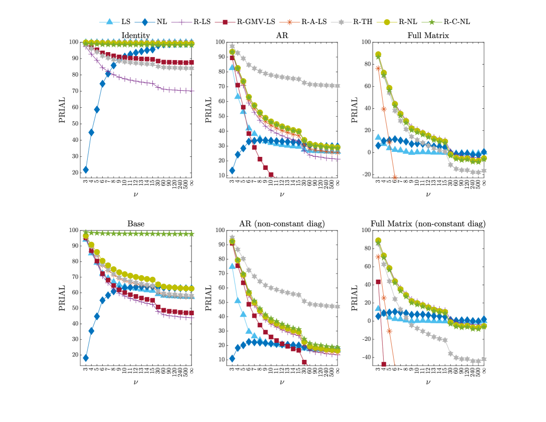
Figure 2: Percentage Relative Improvement in Average Loss (PRIAL) for various dispersion matrix structures, $\nu\in\{3,4,\dots,14,15,30,60,90,120,240,500,\infty\}$, $p=200$ and $n=300$. The plots are scaled such that they extend to $100$ and NL and R-C-NL are fully visible.

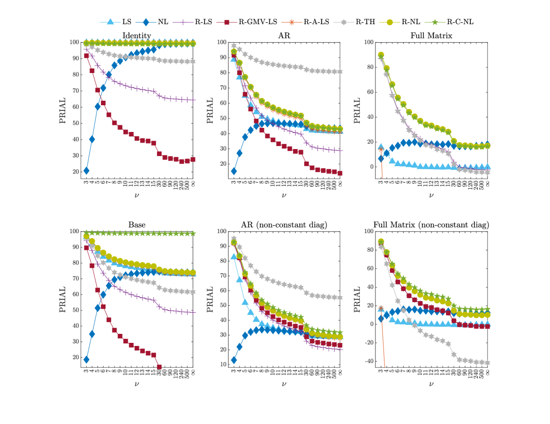
Figure 3: Percentage Relative Improvement in Average Loss (PRIAL) for various dispersion matrix structures, $\nu\in\{3,4,\dots,14,15,30,60,90,120,240,500,\infty\}$, $p=400$ and $n=300$. The plots are scaled such that they extend to $100$ and NL and R-C-NL are fully visible.

5 Empirical Study

From the Center for Research in Security Prices (CRSP) we download daily simple percentage returns of the NYSE, AMEX, and NASDAQ stock exchanges, see https://www.crsp.org/node/1/activetab%3Ddocs for a documentation. The historical data ranges from 02.01.1976 until 31.12.2020 and contains $p^{*}=23^{\prime}131$ stocks in total. The outline of the empirical section is inspired by De Nard et al., (2019).

We conduct a rolling window type exercise, where we consider an estimation window of one year (252 days) and another one with five years (1260 days). In each rolling window we estimate the covariance matrix and perform a minimum variance portfolio optimization with no short selling limits. In the unconstrained case, the global minimum variance portfolio problem is formulated as

$$\min\limits_{\tilde{w}}\tilde{w}^{\top}\boldsymbol{\hat{\Sigma}}\tilde{w}$$

$$\text{subject to}\quad\tilde{w}^{\top}\mathbbm{1}=1~{},$$

where $\mathbbm{1}$ denotes a conformable vector of ones. In the absence of any short-sales constraints the problem has the analytical solution

$$w\mathrel{\vbox{\hbox{\scriptsize.}\hbox{\scriptsize.}}}=\frac{\boldsymbol{\hat{\Sigma}}^{-1}\mathbbm{1}}{\mathbbm{1}^{\top}\boldsymbol{\hat{\Sigma}}^{-1}\mathbbm{1}}~{}.$$

The resulting number of shares (rather than portfolio weights) are then kept fixed for the following 21 days (out-of-sample window). Afterwards the rolling window moves forward by 21 days, the covariance matrix is re-estimated and the weights are updated accordingly. In short, we rebalance the portfolio once a ‘month’, and there are no transaction costs during the ‘month’, where our definition of a ‘month’ corresponds to 21 consecutive trading days rather than a calendar month. Depending on the size of the estimation window, the out-of-sample period starts on 14-Jan-1977 respectively 13-Jan-1981. This results in 528 respectively 480 out-of-sample months. In each month we only consider stocks which have no more than 32 days of missing values during the estimation window and a complete return in the out-of-sample window. The missing values in the remaining universe are set to $0$. Further, every month, only the $p$ stocks with the highest market capitalization are considered, where $p~{}\in~{}\{100,500,1000\}$.

The solution of the minimum variance portfolio only depends on the second moment, that is, the covariance matrix. Therefore, as a portfolio evaluation criterion, the out-of-sample standard deviation is the leading criterion of interest. Hence, in the main text we consider the following two portfolio performance measures:

• SD: annualized standard deviation of portfolio returns.

• TO: average monthly turnover given by

  $$\text{TO}\mathrel{\vbox{\hbox{\scriptsize.}\hbox{\scriptsize.}}}=\frac{1}{(\tau-1)}\sum_{h=1}^{\tau-1}\sum_{j=1}^{p^{*}}\mid w_{j,h+1}-w_{j,h}^{\text{hold}}\mid~{},$$

  Here $p^{*}$ denotes the size of the ‘combined’ investment universe over both months, $h$ and $h+1$; in general some stocks leave the universe, while the same number of new stocks enter the universe, as one advances from month $h$ to month $h+1$ such that $p^{*}\geq p$. Furthermore, $\tau$ denotes the number of out-of-sample months (528 and 480, respectively) and

  $$w_{j,h}^{\text{hold}}\mathrel{\vbox{\hbox{\scriptsize.}\hbox{\scriptsize.}}}=\frac{w_{j,h}\alpha_{j,h}}{\sum_{j=1}^{p^{*}}w_{j,h}\alpha_{j,h}}~{},$$

  with

  $$\alpha_{j,h}\mathrel{\vbox{\hbox{\scriptsize.}\hbox{\scriptsize.}}}=\prod_{s=0}^{20}(1+r_{j,t_{h}+s})$$

  representing the return evolution in the days of month $h$. Note: if stock $j$ is not contained in the universe during month $h$, we set $w_{j,h}=0$ and $r_{j,t_{h}+s}=0\ \forall\ s\in\{0,1,\dots,20\}$.

We consider the same competitors as in Section 4, with one exception: We remove the thresholding method “R-TH”, since the matrix inverse necessary for the portfolio optimization cannot always be computed. We also add the (scaled) sample covariance matrix $\mathbf{\hat{S}}$, which we denote with $S$.

Additionally, in order to test whether the difference of the out-of-sample standard deviation between NL and R-C-NL is significantly different from zero, we apply the HAC inference of Ledoit and Wolf, (2011).

Table 2 presents the main results; for additional results pertaining to alternative performance measures, see Appendix A. The findings are as follows:

• R-C-NL has the lowest SD in every scenario.

• R-C-NL has a significantly lower SD than NL in every scenario.

• R-NL has a lower SD than NL, except for $p=1000$, where they have a similar SD.

• The difference in SD between R-NL and R-C-NL increases as $p$ increases.

• For both $n=252$ and $n=1260$, the robust estimators have a lower SD than the non-robust estimators when $p$ is small. For large $p$ the non-robust estimators perform similarly or better than the robust estimators. This holds for linear shrinkage and nonlinear shrinkage estimators; an exception is R-GMV-LS in the case $n=1260$.

• For $p=500$ and $p=1000$, NL always outperforms the robust linear shrinkage estimators.

• For $p=100$, NL and the robust linear shrinkage estimators perform similarly.

• Except for the case $p=100$, R-C-NL has the lowest TO in every scenario.

• R-NL always has lower TO than NL.

We note that the improvement of R-NL over NL in terms of SD is relatively small, and indeed substantial improvements in SD only occur for R-C-NL. In other words, the strongest improvement appears to stem from using NL on the correlation matrix. However, NL is known to be a very strong benchmark in unconstrained PF optimization. Consequently, already the comparatively small gain of R-NL over NL leads to the lowest SD in five out of six considered scenarios.

Table 2: Out-of-sample portfolio statistics for the largest $p$ stocks on CRSP and an estimation window of $n=252$ and $n=1260$ days, respectively. Significant outperformance of the introduced R-C-NL estimator over NL in terms of SD is indicated by asterisks: ** indicates significance at the 0.05 level and *** indicates significance at the 0.01 level.

	S	LS	NL	R-LS	R-GMV-LS	R-A-LS	R-NL	R-C-NL
	$n=252$
	$p=100$
SD	$13.41$	$12.36$	$11.91$	$12.29$	$11.91$	$12.20$	$11.86$	${\color[rgb]{0,0,1}11.60}\text{***}$
TO	$2.23$	$1.40$	$1.02$	$1.38$	${\color[rgb]{0,0,1}0.79}$	$1.25$	$0.91$	$0.86$
	$p=500$
SD	$-$	$9.65$	$9.10$	$10.01$	$9.41$	$9.65$	$9.08$	${\color[rgb]{0,0,1}8.49}\text{***}$
TO	$-$	$2.29$	$1.16$	$2.72$	$1.59$	$2.18$	$1.04$	${\color[rgb]{0,0,1}1.03}$
	$p=1000$
SD	$-$	$8.33$	$8.23$	$8.38$	$8.45$	$8.34$	$8.23$	${\color[rgb]{0,0,1}7.04}\text{***}$
TO	$-$	$1.59$	$1.01$	$1.76$	$0.93$	$1.56$	$0.92$	${\color[rgb]{0,0,1}0.90}$
	$n=1260$
	$p=100$
SD	$12.83$	$12.78$	$12.68$	$12.67$	$12.69$	$12.68$	$12.59$	${\color[rgb]{0,0,1}12.55}\text{**}$
TO	$0.65$	$0.60$	$0.57$	$0.54$	${\color[rgb]{0,0,1}0.38}$	$0.53$	$0.49$	$0.48$
	$p=500$
SD	$10.25$	$9.82$	$9.35$	$9.72$	$9.44$	$9.69$	$9.32$	${\color[rgb]{0,0,1}9.12}\text{***}$
TO	$1.97$	$1.53$	$0.92$	$1.45$	$0.72$	$1.41$	$0.79$	${\color[rgb]{0,0,1}0.67}$
	$p=1000$
SD	$12.55$	$8.91$	$8.04$	$9.04$	$8.12$	$8.91$	$8.05$	${\color[rgb]{0,0,1}7.46}\text{***}$
TO	$6.56$	$2.38$	$0.94$	$2.52$	$0.84$	$2.35$	$0.80$	${\color[rgb]{0,0,1}0.64}$

6 Conclusion

This paper combines nonlinear shrinkage with Tyler’s method, thereby creating a fast and stable algorithm to estimate the dispersion matrix in elliptical models; the resulting estimator is robust against both heavy tails and high dimensions. We developed the algorithm by separating calculation of the eigenvalues and the eigenvectors and showed that eigenvectors could be obtained by an iterative procedure. We also showed that the resulting R-NL estimator is still rotation-equivariant, although it no longer is contained in the Steinian class of rotation-equivariant estimators that keeps the vectors of the sample covariance matrix and only shrinks the sample eigenvalues. We also compared our approach to existing methods from the literature using both extensive simulations and an application to real data, showcasing its favorable performance. Last but not least, it turns out that a further performance boost can be obtained by using our method on scaled data, which basically amounts to separating the problem of estimating a covariance matrix into estimation of individual variances and estimation of the correlation matrix; the resulting estimator is called R-C-NL.

Appendix A Further Empirical and Simulation Results

Figures 4 and 5 show the simulation results for $n=150$ and $p=100$ and $p=200$ respectively. Figure 6 compares with the “SRTy” estimator of Breloy et al., (2019), by using the NL shrinkage eigenvalues as target eigenvalues. That is, the target matrix of eigenvalues is given as $\boldsymbol{\Lambda}_{0}$ as in the main paper. The shrinkage strength $\beta$ is given by

$$\beta\mathrel{\vbox{\hbox{\scriptsize.}\hbox{\scriptsize.}}}=\frac{\alpha}{1+\alpha},$$

in Breloy et al., (2019), so that $\beta=0$ corresponds to no shrinkage, whereas $\beta=1$ corresponds to maximal shrinkage (or setting $\alpha=\infty$).

Interestingly, in all but the settings (F) and (F’), setting $\beta=1$, and thus maximally shrinking towards $\boldsymbol{\Lambda}_{0}$ appears beneficial. In fact, the performance in this settings of $\beta=1$ is about the same as R-NL. However, in the settings (F) and (F’), the situation is reversed and performance gets worse, the higher $\beta$ is chosen. With the additional updating step performed in R-NL, performance is about the same as choosing $\beta=0$, showing that R-NL can have a substantial benefit over using SRTy with $\beta=1$.

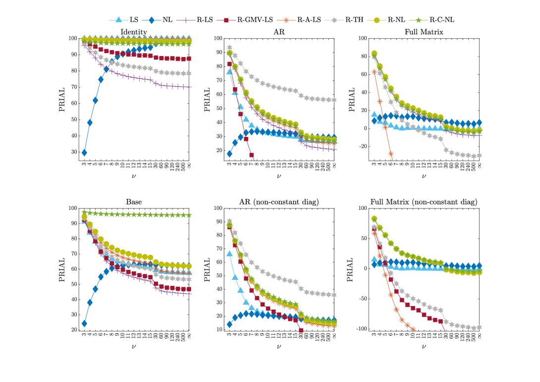
Figure 4: Percentage Relative Improvement in Average Loss (PRIAL) for various dispersion matrix structures, $\nu\in\{3,4,\dots,14,15,30,60,90,120,240,500,\infty\}$, $p=100$ and $n=150$. The plots are scaled such that they extend to $100$ and NL and R-C-NL are fully visible.

Figure 5: Percentage Relative Improvement in Average Loss (PRIAL) for various dispersion matrix structures, $\nu\in\{3,4,\dots,14,15,30,60,90,120,240,500,\infty\}$, $p=200$ and $n=150$. The plots are scaled such that they extend to $100$ and NL and R-C-NL are fully visible.

Figure 6: Percentage Relative Improvement in Average Loss (PRIAL) for various dispersion matrix structures, $\nu\in\{3,4,\dots,14,15,30,60,90,120,240,500,\infty\}$, $p=200$ and $n=300$.

For our empirical application in Section 5 of the main paper, the following four additional performance measures are reported:

• AV: annualized average simple percentage portfolio return.

• TR: final cumulative simple percentage portfolio return.

• MD: percentage maximum drawdown given by

  $$\text{MD}\mathrel{\vbox{\hbox{\scriptsize.}\hbox{\scriptsize.}}}=\max_{\bar{t}\in(0,n)}\left(\max_{t\in(0,\bar{t})}\left[\frac{\tilde{R}_{t}-\tilde{R}_{\tilde{t}}}{\tilde{R}_{t}}\right]\right)~{},$$

  where $\tilde{R}_{t}$ is the cumulative simple percentage portfolio return at day $t$.

• IR: annualized information ratio given by

  $$IR\mathrel{\vbox{\hbox{\scriptsize.}\hbox{\scriptsize.}}}=\frac{AV}{SD}~{}.$$

Table 3: Additional out-of-sample portfolio statistics for the daily $p$ largest stocks on CRSP and an estimation window of $n=252$ and $n=1260$ days, respectively.

	S	LS	NL	R-LS	R-GMV-LS	R-A-LS	R-NL	R-C-NL
	$n=252$
	$p=100$
IR	$0.69$	$0.80$	$0.87$	$0.81$	$0.87$	$0.82$	$0.87$	$0.91$
AV	$9.24$	$9.94$	$10.31$	$9.97$	$10.37$	$9.97$	$10.32$	$10.55$
TR	$3,813.45$	$5,548.60$	$6,710.69$	$5,641.21$	$6,902.58$	$5,677.55$	$6,767.45$	$7,607.62$
MD	$46.56$	$35.20$	$38.48$	$37.94$	$33.40$	$37.05$	$35.48$	$33.26$
	$p=500$
IR	$-$	$1.17$	$1.21$	$1.16$	$1.20$	$1.20$	$1.22$	$1.35$
AV	$-$	$11.27$	$11.01$	$11.57$	$11.26$	$11.56$	$11.07$	$11.50$
TR	$-$	$11,493.55$	$10,447.08$	$12,921.46$	$11,521.84$	$13,053.61$	$10,776.80$	$13,303.94$
MD	$-$	$29.41$	$29.24$	$29.92$	$30.33$	$28.56$	$30.61$	$28.22$
	$p=1000$
IR	$-$	$1.47$	$1.44$	$1.46$	$1.42$	$1.46$	$1.43$	$1.74$
AV	$-$	$12.21$	$11.87$	$12.23$	$12.04$	$12.21$	$11.76$	$12.22$
TR	$-$	$18,342.65$	$15,877.34$	$18,502.15$	$16,942.34$	$18,347.06$	$15,080.18$	$19,254.29$
MD	$-$	$33.88$	$34.39$	$34.52$	$34.82$	$33.63$	$35.19$	$26.75$
	$n=1260$
	$p=100$
IR	$0.93$	$0.94$	$0.94$	$0.94$	$0.95$	$0.94$	$0.93$	$0.95$
AV	$11.95$	$12.06$	$11.97$	$11.89$	$12.01$	$11.90$	$11.74$	$11.86$
TR	$8,428.17$	$8,863.69$	$8,585.57$	$8,323.75$	$8,709.89$	$8,341.21$	$7,862.18$	$8,267.73$
MD	$39.08$	$37.83$	$38.08$	$36.21$	$34.00$	$36.12$	$35.31$	$34.98$
	$p=500$
IR	$1.08$	$1.14$	$1.21$	$1.16$	$1.24$	$1.17$	$1.23$	$1.30$
AV	$11.04$	$11.23$	$11.33$	$11.23$	$11.67$	$11.30$	$11.47$	$11.82$
TR	$6,599.24$	$7,256.96$	$7,703.75$	$7,271.52$	$8,779.64$	$7,487.65$	$8,162.71$	$9,462.95$
MD	$33.16$	$31.64$	$32.92$	$30.85$	$31.07$	$30.79$	$31.48$	$31.56$
	$p=1000$
IR	$0.93$	$1.37$	$1.52$	$1.37$	$1.53$	$1.39$	$1.53$	$1.67$
AV	$11.71$	$12.23$	$12.26$	$12.38$	$12.46$	$12.38$	$12.29$	$12.50$
TR	$7,799.17$	$11,257.77$	$11,731.10$	$11,893.95$	$12,676.34$	$11,951.51$	$11,857.04$	$13,137.98$
MD	$37.38$	$33.98$	$32.18$	$33.42$	$32.07$	$33.58$	$32.28$	$27.65$

References

- Abramovich and Spencer, (2007) Abramovich, Y. I. and Spencer, N. K. (2007). Diagonally loaded normalised sample matrix inversion (LNSMI) for outlier-resistant adaptive filtering. In 2007 IEEE International Conference on Acoustics, Speech and Signal Processing – ICASSP ’07, volume 3, pages III–1105–III–1108.
- Absil et al., (2007) Absil, P.-A., Mahony, R., and Sepulchre, R. (2007). Optimization Algorithms on Matrix Manifolds. Princeton University Press, USA.
- Ashurbekova et al., (2021) Ashurbekova, K., Usseglio-Carleve, A., Forbes, F., and Achard, S. (2021). Optimal shrinkage for robust covariance matrix estimators in a small sample size setting. https://hal.archives-ouvertes.fr/hal-02378034.
- Auguin et al., (2016) Auguin, N., Morales-Jimenez, D., McKay, M., and Couillet, R. (2016). Robust shrinkage -estimators of large covariance matrices. In 2016 IEEE Statistical Signal Processing Workshop (SSP), pages 1–4.
- (5) Bickel, P. J. and Levina, E. (2008a). Covariance regularization by thresholding. Annals of Statistics, 36(6):2577 – 2604.
- (6) Bickel, P. J. and Levina, E. (2008b). Regularized estimation of large covariance matrices. Annals of Statistics, 36(1):199 – 227.
- Breloy et al., (2019) Breloy, A., Ollila, E., and Pascal, F. (2019). Spectral shrinkage of Tyler’s -estimator of covariance matrix. In 2019 IEEE 8th International Workshop on Computational Advances in Multi-Sensor Adaptive Processing (CAMSAP), pages 535–538.
- Cai and Liu, (2011) Cai, T. and Liu, W. (2011). Adaptive thresholding for sparse covariance matrix estimation. Journal of the American Statistical Association, 106(494):672–684.
- Cambanis et al., (1981) Cambanis, S., Huang, S., and Simons, G. (1981). On the theory of elliptically contoured distributions. Journal of Multivariate Analysis, 11(3):368–385.
- Chen et al., (2011) Chen, Y., Wiesel, A., and Hero, A. O. (2011). Robust shrinkage estimation of high-dimensional covariance matrices. IEEE Transactions on Signal Processing, 59(9):4097–4107.
- Couillet and McKay, (2014) Couillet, R. and McKay, M. (2014). Large dimensional analysis and optimization of robust shrinkage covariance matrix estimators. Journal of Multivariate Analysis, 131:99–120.
- Danon and Garber, (2022) Danon, L. and Garber, D. (2022). Frank-Wolfe-based algorithms for approximating Tyler’s -estimator. In Advances in Neural Information Processing Systems, volume 35, pages 3637–3648.
- De Nard et al., (2022) De Nard, G., Engle, R. F., Ledoit, O., and Wolf, M. (2022). Large dynamic covariance matrices: Enhancements based on intraday data. Journal of Banking and Finance, 138:106426.
- De Nard et al., (2019) De Nard, G., Ledoit, O., and Wolf, M. (2019). Factor models for portfolio selection in large dimensions: The good, the better and the ugly. Journal of Financial Econometrics, 19(2):236–257.
- Donoho et al., (2018) Donoho, D., Gavish, M., and Johnstone, I. (2018). Optimal shrinkage of eigenvalues in the spiked covariance model. Annals of Statistics, 46(4):1742 – 1778.
- Engle et al., (2019) Engle, R. F., Ledoit, O., and Wolf, M. (2019). Large dynamic covariance matrices. Journal of Business & Economic Statistics, 37(2):363–375.
- Fang et al., (1990) Fang, K., Kotz, S., and Ng, K. (1990). Symmetric Multivariate and Related Distributions. Number 36 in Monographs on Statistics and Applied Probability. Chapman & Hall, New York.
- Goes et al., (2020) Goes, J., Lerman, G., and Nadler, B. (2020). Robust sparse covariance estimation by thresholding Tyler’s -estimator. Annals of Statistics, 48(1):86 – 110.
- Hediger and Näf, (2022) Hediger, S. and Näf, J. (2022). Combining the MGHyp distribution with nonlinear shrinkage in modeling financial asset returns. Available at SSRN 4069441.
- Johnstone, (2001) Johnstone, I. M. (2001). On the distribution of the largest eigenvalue in principal components analysis. Annals of Statistics, 29(2):295 – 327.
- Johnstone and Lu, (2009) Johnstone, I. M. and Lu, A. Y. (2009). On consistency and sparsity for principal components analysis in high dimensions. Journal of the American Statistical Association, 104(486):682–693. PMID: 20617121.
- Ke et al., (2019) Ke, Y., Minsker, S., Ren, Z., Sun, Q., and Zhou, W.-X. (2019). User-friendly covariance estimation for heavy-tailed distributions. Statistical Science, 34(3):454–471.
- Kent and Tyler, (1991) Kent, J. T. and Tyler, D. E. (1991). Redescending -estimates of multivariate location and scatter. Annals of Statistics, 19(4):2102–2119.
- Ledoit and Wolf, (2004) Ledoit, O. and Wolf, M. (2004). A well-conditioned estimator for large-dimensional covariance matrices. Journal of Multivariate Analysis, 88(2):365–411.
- Ledoit and Wolf, (2011) Ledoit, O. and Wolf, M. (2011). Robust performance hypothesis testing with the variance. Wilmott, 2011(55):86–89.
- Ledoit and Wolf, (2012) Ledoit, O. and Wolf, M. (2012). Nonlinear shrinkage estimation of large-dimensional covariance matrices. Annals of Statistics, 40(2):1024–1060.
- Ledoit and Wolf, (2015) Ledoit, O. and Wolf, M. (2015). Spectrum estimation: A unified framework for covariance matrix estimation and pca in large dimensions. Journal of Multivariate Analysis, 139:360–384.
- Ledoit and Wolf, (2020) Ledoit, O. and Wolf, M. (2020). Analytical nonlinear shrinkage of large-dimensional covariance matrices. Annals of Statistics, 48(5):3043–3065.
- (29) Ledoit, O. and Wolf, M. (2022a). The power of (non-)linear shrinking: A review and guide to covariance matrix estimation. Journal of Financial Econometrics, 20(1):187–218.
- (30) Ledoit, O. and Wolf, M. (2022b). Quadratic shrinkage for large covariance matrices. Bernoulli, 28(3):1519–1547.
- Okamoto, (1973) Okamoto, M. (1973). Distinctness of the eigenvalues of a quadratic form in a multivariate sample. Annals of Statistics, 1(4):763–765.
- Ollila et al., (2021) Ollila, E., Palomar, D. P., and Pascal, F. (2021). Shrinking the eigenvalues of -estimators of covariance matrix. IEEE Transactions on Signal Processing, 69:256–269.
- Ollila and Tyler, (2014) Ollila, E. and Tyler, D. E. (2014). Regularized -estimators of scatter matrix. IEEE Transactions on Signal Processing, 62(22):6059–6070.
- Razaviyayn et al., (2013) Razaviyayn, M., Hong, M., and Luo, Z.-Q. (2013). A unified convergence analysis of block successive minimization methods for nonsmooth optimization. SIAM Journal on Optimization, 23(2):1126–1153.
- Rothman et al., (2009) Rothman, A. J., Levina, E., and Zhu, J. (2009). Generalized thresholding of large covariance matrices. Journal of the American Statistical Association, 104(485):177–186.
- Stein, (1975) Stein, C. (1975). Estimation of a covariance matrix. Rietz lecture, 39th Annual Meeting IMS. Atlanta, Georgia.
- Stein, (1986) Stein, C. (1986). Lectures on the theory of estimation of many parameters. Journal of Mathematical Sciences, 34(1):1373–1403.
- Sun et al., (2014) Sun, Y., Babu, P., and Palomar, D. P. (2014). Regularized Tyler’s scatter estimator: Existence, uniqueness, and algorithms. IEEE Transactions on Signal Processing, 62(19):5143–5156.
- (39) Tyler, D. E. (1987a). A distribution-free -estimator of multivariate scatter. Annals of Statistics, 15(1):234–251.
- (40) Tyler, D. E. (1987b). Statistical analysis for the angular central Gaussian distribution on the sphere. Biometrika, 74(3):579–589.
- Wen and Yin, (2013) Wen, Z. and Yin, W. (2013). A feasible method for optimization with orthogonality constraints. Mathematical Programming, 142(1):397–434.
- Wiesel, (2012) Wiesel, A. (2012). Unified framework to regularized covariance estimation in scaled Gaussian models. IEEE Transactions on Signal Processing, 60(1):29–38.
- Yang et al., (2014) Yang, L., Couillet, R., and McKay, M. R. (2014). Minimum variance portfolio optimization with robust shrinkage covariance estimation. In 2014 48th Asilomar Conference on Signals, Systems and Computers, pages 1326–1330. IEEE.
- Yi and Tyler, (2021) Yi, M. and Tyler, D. E. (2021). Shrinking the covariance matrix using convex penalties on the matrix-log transformation. Journal of Computational and Graphical Statistics, 30(2):442–451.
- Yu et al., (2017) Yu, P. L., Wang, X., and Zhu, Y. (2017). High dimensional covariance matrix estimation by penalizing the matrix-logarithm transformed likelihood. Computational Statistics & Data Analysis, 114(C):12–25.
- Zhang and Wiesel, (2016) Zhang, T. and Wiesel, A. (2016). Automatic diagonal loading for Tyler’s robust covariance estimator. In 2016 IEEE Statistical Signal Processing Workshop (SSP), pages 1–5. IEEE.