TuneUp: A Simple Improved Training Strategy for Graph Neural Networks

Abstract

Despite recent advances in Graph Neural Networks (GNNs), their training strategies remain largely under-explored. The conventional training strategy learns over all nodes in the original graph(s) equally, which can be sub-optimal as certain nodes are often more difficult to learn than others. Here we present TuneUp, a simple curriculum-based training strategy for improving the predictive performance of GNNs. TuneUp trains a GNN in two stages. In the first stage, TuneUp applies conventional training to obtain a strong base GNN. The base GNN tends to perform well on head nodes (nodes with large degrees) but less so on tail nodes (nodes with small degrees). Therefore, the second stage of TuneUp focuses on improving prediction on the difficult tail nodes by further training the base GNN on synthetically generated tail node data. We theoretically analyze TuneUp and show it provably improves generalization performance on tail nodes. TuneUp is simple to implement and applicable to a broad range of GNN architectures and prediction tasks. Extensive evaluation of TuneUp on five diverse GNN architectures, three types of prediction tasks, and both transductive and inductive settings shows that TuneUp significantly improves the performance of the base GNN on tail nodes, while often even improving the performance on head nodes. Altogether, TuneUp produces up to 57.6% and 92.2% relative predictive performance improvement in the transductive and the challenging inductive settings, respectively.

Introduction

Graph Neural Networks (GNNs) are one of the most successful and widely used paradigms for representation learning on graphs, achieving state-of-the-art performance on a variety of prediction tasks, such as semi-supervised node classification (Kipf and Welling 2017; Velickovic et al. 2018), link prediction (Hamilton, Ying, and Leskovec 2017; Kipf and Welling 2016), and recommender systems (Ying et al. 2018; He et al. 2020). There has been a surge of work on improving GNN model architectures (Velickovic et al. 2018; Xu et al. 2019, 2018; Shi et al. 2020; Klicpera, Bojchevski, and Günnemann 2019; Wu et al. 2019; Zhao and Akoglu 2019; Li et al. 2019; Chen et al. 2020; Li et al. 2021) and task-specific losses (Kipf and Welling 2016; Rendle et al. 2012; Verma et al. 2021; Huang et al. 2021b). Despite all these advances, strategies for training a GNN on a given supervised loss remain largely under-explored. Existing work has focused on minimizing the given loss averaged over nodes in the original graph(s), which neglects the fact that some nodes are more difficult to learn than others.

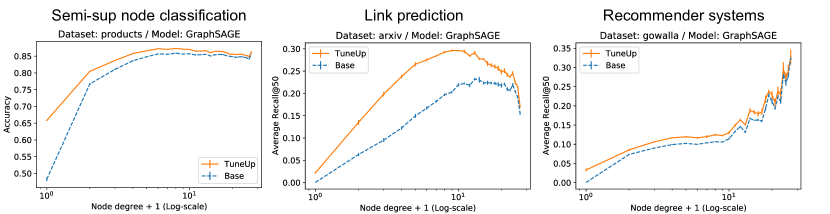
Figure 1: Degree-specific predictive performance of the base GNN (trained with conventional training) and TuneUp GNN in the transductive setting. Between “Base” and “TuneUp”, only the training strategy differs; the model architecture and the loss function stay exactly the same. The $x$-axis represents the node degrees in the training graph, and the $y$-axis is the predictive performance averaged over nodes with specific degrees. We see from the dotted blue curves that the base GNN tends to perform poorly on tail nodes, i.e., nodes with small degrees. Our TuneUp (denoted by the solid orange curves) gives more accurate GNNs than conventional training (“Base”). TuneUp improves the predictive performance across almost all node degrees, but most significantly on tail nodes.

Here we present TuneUp, a simple improved training strategy for improving the predictive performance of GNNs. The key motivation behind TuneUp is that GNNs tend to under-perform on tail nodes, i.e., nodes with small (e.g., 0–5) node degrees, due to the scarce neighbors to aggregation features from (Liu, Nguyen, and Fang 2021). Improving GNN performance on tail nodes is important since they are prevalent in real-world scale-free graphs (Clauset, Shalizi, and Newman 2009) as well as newly arriving cold-start nodes (Lika, Kolomvatsos, and Hadjiefthymiades 2014).

The key idea of TuneUp is to adopt curriculum-based training (Bengio et al. 2009), where it first trains a GNN to perform well on relatively-easy head nodes. It then proceeds to further train the GNN to perform well on the more difficult tail nodes by minimizing the loss over supervised tail node data that is synthetically generated via pseudo-labeling and dropping edges (Rong et al. 2020).

We theoretically analyze TuneUp and show that it provably improves the generalization performance on tail nodes by utilizing information from head nodes. Our theory also justifies how TuneUp generates supervised synthetic tail nodes in the second stage. Our theory suggests that both pseudo-labeling and dropping edges are crucial for improved generalization.

TuneUp is simple to implement on top of the conventional training pipeline of GNNs, as shown in Algorithm 1. Thanks to its simplicity, TuneUp can be readily used with a wide range of GNN models and supervised losses; hence, applicable to many node and edge-level prediction tasks. This is in contrast with recent methods for improving GNN performance on tail nodes (Liu, Nguyen, and Fang 2021; Zheng et al. 2022; Zhang et al. 2022; Kang et al. 2022) as they all require non-trivial modifications of both GNN architectures and loss, making them harder to implement and not applicable to diverse prediction tasks.

To demonstrate the effectiveness and broad applicability of TuneUp, we perform extensive experiments on a wide range of settings. We consider five diverse GNN architectures, three types of key prediction tasks (semi-supervised node classification, link prediction, and recommender systems) with a total of six datasets, as well as both transductive (i.e., prediction on nodes seen during training) and inductive (i.e., prediction on new nodes not seen during training) settings. For the inductive setting, we additionally consider the challenging cold-start scenario (i.e., limited edge connectivity from new nodes) by randomly removing certain portions of edges from new nodes.

Across the settings, TuneUp produces consistent improvement in the predictive performance of GNNs. In the transductive setting, TuneUp significantly improves the performance of base GNNs on tail nodes, while oftentimes even improving the performance on head nodes (see Figure 1). In the inductive setting, TuneUp especially shines in the cold-start prediction scenario, where new nodes are tail-like, producing up to 92.2% relative improvement in the predictive performance. Moreover, our TuneUp significantly outperforms the recent specialized methods for tail nodes (Liu, Nguyen, and Fang 2021; Zheng et al. 2022; Zhang et al. 2022; Kang et al. 2022), while not requiring any modification to GNN architectures nor losses. Overall, our work shows that even a simple training strategy can yield a surprisingly large improvement in the predictive performance of GNNs, pointing to a promising direction to investigate effective training strategies for GNNs, beyond architectures and losses.

General Setup and Conventional Training

Here we introduce a general task setup for machine learning on graphs and review the conventional training strategy of GNNs.

General Setup

We are given a graph $G=(V,E)$, with a set of nodes $V$ and edges $E$, possibly associated with some features. A GNN $F_{\theta}$, parameterized by $\theta$, takes the graph $G$ as input and makes prediction $\widehat{Y}$ for the task of interest. The loss function $L$ measures the discrepancy between the GNN’s prediction $\widehat{Y}$ and the target supervision $Y$. When input node features are available, GNN $F_{\theta}$ can make not only transductive predictions, i.e., prediction over existing nodes $V$, but also inductive predictions (Hamilton, Ying, and Leskovec 2017), i.e., prediction over new nodes $V_{\rm new}$ that are not yet present in $V$. This is a general task setup that covers many representative predictive tasks over graphs as special cases:

Semi-supervised node classification (Kipf and Welling 2017)

• Graph $G$: A graph with input node features.

• Supervison $Y$: Class labels of labeled nodes $V_{\rm labeled}\subset V$.

• GNN $F_{\theta}$: A model that takes $G$ as input and predicts class probabilities over $V$.

• Prediction $\widehat{Y}$: The GNN’s prediction over $V_{\rm labeled}$.

• Loss $L$: Cross-entropy loss.

Link prediction (Kipf and Welling 2016)

• Graph $G$: A graph with input node features.

• Supervison $Y$: Whether node $s\in V$ is linked to node $t\in V$ in $G$ (positive) or not (negative).

• GNN $F_{\theta}$: A model that takes $G$ as input and predicts the score for a pair of nodes $(s,t)\in V\times V$. Specifically, the model generates embedding $\bm{z}_{v}$ for each node in $v\in V$ and uses an MLP over the Hadamard product between $\bm{z}_{s}$ and $\bm{z}_{t}$ to predict the score for the pair $(s,t)$ (Grover and Leskovec 2016).

• Prediction $\widehat{Y}$: The GNN’s predicted scores over $V\times V$.

• Loss $L$: The Bayesian Personalized Ranking (BPR) loss (Rendle et al. 2012), which encourages the predicted score for the positive pair $(s,t_{\rm pos})$ to be higher than that for the negative pair $(s,t_{\rm neg})$ for each source node $s\in V$.

Recommender systems (Wang et al. 2019)

A recommender system is link prediction between user nodes $V_{\rm user}$ and item nodes $V_{\rm item}$.

• Graph $G$: User-item bipartite graph without input node features.

• Supervison $Y$: Whether a user node $u$ has interacted with an item node $v$ in $G$ (positive) or not (negative).

• GNN $F_{\theta}$: A model that takes $G$ as input and predicts the score for a pair of nodes $(u,v)\in V_{\rm user}\times V_{\rm item}$. Following Wang et al. (2019), GNN parameter $\theta$ contains the input shallow embeddings in addition to the original message passing GNN parameter. To produce the score for the pair of nodes $(u,v)$, we generate the user and item embeddings, $\bm{z}_{u}$ and $\bm{z}_{v}$, and take the inner product $\bm{z}_{u}^{\top}\bm{z}_{v}$ to compute the score (Wang et al. 2019).

• Prediction $\widehat{Y}$: The GNN’s predicted scores over $V_{\rm user}\times V_{\rm item}$.

• Loss $L$: The BPR loss (Rendle et al. 2012).

Conventional GNN Training

A conventional way to train a GNN (Kipf and Welling 2017) is to minimize the loss $L(\widehat{Y},Y)$ via gradient descent, as shown in L2–5 of Algorithm1. Extension to mini-batch training (Hamilton, Ying, and Leskovec 2017; Zeng et al. 2020) is straightforward by sampling subgraph $G$ in each parameter update.

Algorithm 1 TuneUp. Compared to the conventional training of a GNN (L2–5), TuneUp introduces a two-stage training process and only adds two components (L8 and L12) that are straightforward to implement. Each parameter update of TuneUp is as efficient as the conventional GNN training.

Given: GNN $F_{\theta}$, graph $G$, loss $L$, supervision $Y$, DropEdge ratio $\alpha$.

1:  # First stage: Conventional training to obtain a base GNN.

2:  while $\theta$ not converged do

3:     Make prediction $\widehat{Y}=F_{\theta}(G)$

4:     Compute loss $L(\widehat{Y},Y)$, compute gradient $\nabla_{\theta}L$, and update parameter $\theta$.

5:  end while

6:  # Set up for the second stage.

7:  if task is semi-supervised node classification then

8:     Use $F_{\theta}$ to predict pseudo-labels on non-isolated, unlabeled nodes. Add the pseudo-labels into $Y$.

9:  end if

10:  # Second stage: Further training the base GNN with increased tail supervision.

11:  while $\theta$ not converged do

12:     Synthesize tail nodes, i.e., randomly drop $\alpha$ of edges: $G\xrightarrow{\rm DropEdge}\widetilde{G}$.

13:     Make prediction $\widehat{Y}=F_{\theta}(\widetilde{G})$.

14:     Compute loss $L(\widehat{Y},Y)$, compute gradient $\nabla_{\theta}L$, and update parameter $\theta$.

15:  end while

Issue with Conventional Training. Conventional training implicitly assumes GNNs can learn over all nodes equally well. In practice, some nodes, such as low-degree tail nodes, are more difficult for GNNs to learn due to the scarce neighborhood information. As a result, GNNs trained with conventional training often give poor predictive performance on the difficult tail nodes (Liu, Nguyen, and Fang 2021).

TuneUp: An Improved GNN Training

To resolve the issue, we present TuneUp, a simple curriculum learning strategy, to improve GNN performance, especially on the difficult tail nodes. At a high level, TuneUp first trains a GNN to perform well on the relatively easy head nodes. Then, it further trains the GNN to also perform well on the more difficult tail nodes.

Specifically, in the first stage (L2–5 in Algorithm 1), TuneUp uses conventional GNN training to obtain a strong base GNN model. The base GNN model tends to perform well on head nodes, but poorly on tail nodes. To remedy this issue, in the second training stage, TuneUp futher trains the base GNN on synthetic tail nodes (L7–L15 in Algorithm 1). TuneUp synthesizes supervised tail node data in two steps, detailed next: (1) synthesizing additional tail node inputs, and (2) adding target supervision on the synthetic tail nodes.

Synthesizing tail node inputs

In many real-world graphs, head nodes start off as tail nodes, e.g., well-cited paper nodes are not cited at the beginning in a paper citation network, and warm users (users with many item interactions) start off as cold-start users in recommender systems. Hence, our key idea is to synthesize tail nodes by systematically removing edges from head nodes. There can be different ways to remove edges. In this work, we simply adopt DropEdge (Rong et al. 2020) to instantiate our idea. DropEdge drops a certain portion (given by hyperparameter $\alpha$) of edges randomly from the original graph $G$ to obtain $\widetilde{G}$ (L12 in Algorithm 1). The resulting $\widetilde{G}$ contains more nodes with low degrees, i.e., tail nodes, than the original graph $G$. Hence, the GNN sees more (synthetic) tail nodes as input during training.

Adding supervision on the synthetic tail nodes

After synthesizing the tail node inputs, TuneUp then adds target supervision (e.g., class labels for node classification, edges for link prediction) on them so that a supervised loss can be computed. Our key idea is to reuse the target labels on the original head nodes for the synthesized tail nodes. The rationale is that many prediction tasks involve target labels that are inherent node properties that do not change with node degree. For example, additional citations will not change a paper’s subject area, and additional purchases will not change a product’s category.

Concretely, for link prediction tasks, TuneUp directly reuses the original edges $E$ in $G$ (before dropping) for the target supervision on the synthetic tail nodes. For semi-supervised node classification, TuneUp can similarly reuse the target labels of labeled nodes $V_{\rm labeled}$ in $G$ as the labels for synthetic tail nodes in $\widetilde{G}$. A critical challenge here is that the number of labeled nodes $V_{\rm labeled}$ is often small in the semi-supervised setting, e.g., 1%–5% of all nodes $V$, limiting the amount of target label supervision TuneUp can reuse.

To resolve this issue, TuneUp applies the base GNN (obtained in the first training stage) over $G$ to predict pseudo-labels (Lee et al. 2013) over non-isolated nodes in $V_{\rm unlabeled}\equiv V\setminus V_{\rm labeled}$. TuneUp then includes the pseudo-labels as supervision $Y$ in the second stage (L8 in Algorithm 1). This significantly increases the size of the supervision $Y$, e.g., by a factor of $\approx$100 if only 1% of nodes are labeled. While the pseudo-labels can be noisy, they are “best guesses” made by the base GNN in the sense that they are predicted using full graph information $G$ as input. In the second stage, TuneUp trains the GNN to maintain its “best guesses” given sparser graph $\widetilde{G}$ as input, which encourages the GNN to perform well on nodes whose neighbors are actually scarce. Note that this strategy is fundamentally different from the classical pseudo-labeling method (Lee et al. 2013) that trains a model without sparsifying the input graph. In the following sections, we will see this both theoretically and empirically.

Theoretical Analysis

To theoretically understand TuneUp with clean insights, we consider node classification with binary labels for a part of a graph with two extreme groups of nodes: ones with full degrees and ones with zero degrees. Considering this part of a graph as an example, we mathematically show how TuneUp uses the nodes with high degrees to improve the generalization for the nodes with low degrees via the curriculum-based training strategy.

We analyze the generalization gap between the test errors of nodes with low degrees and the training errors of nodes with high degrees. This type of generalization is non-standard and does not necessarily happen unless we take advantage of some additional mechanisms such as dropping edges. Define $d$ to be the dimensionality of the feature space of the last hidden layer of a GNN. Denote by $m$ the size of a set of labeled nodes used for training. Let $Q$ be the average training loss at the end of the first stage of TuneUp curriculum learning.

We prove a theorem (Theorem 1), which shows the following three statements:

1. First, consider TuneUp without pseudo labeling (denoted by $M_{1}$). $M_{1}$ helps reduce the test errors of nodes with low degrees via utilizing the nodes with high degrees by dropping edges: i.e., the generalization bound in our theorem decreases towards zero at the rate of $\sqrt{\frac{d}{m}}$.

2. The full TuneUp (denoted by $M_{2}$) further reduces the test errors of nodes with low degrees by utilizing pseudo-labels: i.e., the rate of$\sqrt{\frac{d}{m}}$ is replaced by the rate of $\sqrt{\frac{1}{m}}+Q$, where typically $Q=0$ as $Q$ is explicitly minimized as a training objective. Thus, curriculum-based training with pseudo-labels can remove the factor $d$.

3. TuneUp without DropEdge (denoted by $M_{3}$), i.e., the classical pseudo-labeling method, degrades the test errors of nodes with low degrees by incurring additional error term $\tau>0$ that measures the difference between the losses with and without edges. This is consistent with the above intuition that generalizing from high-degree training nodes to the low-degree test nodes requires some relationship between ones with and without edges.

For each method $M\in\{M_{i}\}_{i=1}^{3}$, we define $\Delta(M)$ to be the generalization gap between the test errors of nodes with low degrees and the training errors of nodes with high degrees.

Theorem 1.

For any $\delta>0$, with probability at least $1-\delta$, the following holds for all $M\in\{M_{1},M_{2},M_{3}\}$:

$$\Delta(M) \leq\sqrt{\frac{\mathbf{1}\{M=M_{1}\}8(d-1)\ln(\frac{16em}{\delta})+8\ln(\frac{16em}{\delta})}{m}}$$

$$\quad+\mathbf{1}\{M\neq M_{1}\}Q+\mathbf{1}\{M=M_{3}\}\tau+G,$$

where $G\rightarrow 0$ as the graph size approaches infinity.

Proof.

A more detailed version of Theorem 1 is presented along with the complete proof in Appendix. ∎

Related Work

Methods for Tail Nodes

Recently, a surge of methods have been developed for improving the predictive performance of GNNs on tail nodes (Liu, Nguyen, and Fang 2021; Zheng et al. 2022; Kang et al. 2022; Zhang et al. 2022). These methods augment GNNs with complicated tail-node-specific architectural components and losses, while TuneUp focuses on the training strategy that does not require any architectural nor loss modification.

Data augmentation for GNNs

The second stage of TuneUp is data augmentation over graphs, on which there has been abundant work (Zhao et al. 2021; Feng et al. 2020; Verma et al. 2021; Kong et al. 2020; Liu et al. 2022; Ding et al. 2022). The most relevant one is DropEdge (Rong et al. 2020), which was originally developed to overcome the over-smoothing issue of GNNs (Li, Han, and Wu 2018) specific to semi-supervised node classification. Our work has a different motivation and expended scope: We use DropEdge to synthesize tail node inputs and consider a wider range of prediction tasks. Our theoretical analysis also differs and focuses on generalization on tail nodes. Methodologically, TuneUp additionally employs curriculum learning and pseudo-labels, both of which are crucial in improving GNN performance over the vanilla DropEdge.

Experiments

We evaluate the broad applicability of TuneUp by considering five GNN models and testing them on the three prediction tasks (semi-supervised node classification, link prediction, and recommender systems) with three predictive settings: transductive, inductive, and cold-start inductive predictions.

Experimental Settings

We evaluate TuneUp on realistic tail node scenarios in both transductive (i.e., naturally occurring tail nodes in scale-free networks) and inductive (i.e., newly arrived cold-start nodes) settings. Conventional experimental setups (Hu et al. 2020; Wang et al. 2019) are not suitable for evaluating TuneUp as they fail to provide either (1) transductive prediction settings with tail nodes, or (2) inductive cold-start prediction settings. Therefore, we split the original realistic graph datasets (Hu et al. 2020; Wang et al. 2019) to simulate both (1) and (2) in a realistic manner. Below, we describe the split for each task type. The dataset statistics are summarized in Table 1.

Table 1: Statistics of nodes used for the transductive evaluation. For link prediction and recommender system graphs (user-item bipartite graphs), we only evaluate on nodes/users with at least one edge in the validation set. See Appendix for the description of the datasets.

Task	Dataset	#Nodes	Avg deg.	Feat. dim
Node	arxiv	143,941	12.93	128
classification	products	2,277,597	48.01	100
Link	flickr	82,981	4.81	500
prediction	arxiv	141,917	7.20	128
Recsys	gowalla	29,858	3.44	–
	amazon-book	52,643	5.67	–

Semi-supervised node classification

Given all nodes in the original dataset, we randomly selected 95% of the nodes and used their induced subgraph as the graph $G=(V,E)$ to train GNNs. The remaining 5% of nodes, $V_{\rm new}$, is used for inductive test prediction. Within $V$, 10% and 2% of the nodes are used as labeled nodes $V_{\rm labeled}$ for arxiv and products, respectively. Half of $V_{\rm labeled}$ is used to compute the supervised training loss, and the other half is used as the transductive validation set for selecting hyperparameters. We used classification accuracy for the evaluation metric. For the transductive performance, we report the test accuracy on the unlabeled test nodes $V_{\rm unlabeled}\equiv V\setminus V_{\rm labeled}$, while for the inductive performance, we report the test accuracy on $V_{\rm new}$. For the inductive test prediction, we also consider the cold-start scenario, where certain portions (30%, 60%, and 90%) of edges are randomly removed from the new nodes.

Table 2: The improvement with TuneUp over the base GNNs for five diverse GNN model architectures. We used the same datasets as Figure 1. For semi-supervised node classification, “inductive (cold)” randomly removed 90% of edges from the new nodes, while for link prediction, 60% were removed. ^†For semi-supervised node classification, GAT gave Out-Of-Memory (OOM) on the products dataset, so we report the performance on arxiv instead.

Task	Config	Setting	SAGE	GCN	SAGE-max	SAGE-sum	GAT
	Transductive	Base	0.8409$\pm$0.0006	0.8432$\pm$0.0007	0.8132$\pm$0.0004	0.7611$\pm$0.0030	OOM / 0.6862$\pm$0.0023†
Semi-sup		TuneUp	0.8552$\pm$0.0003	0.8523$\pm$0.0007	0.8373$\pm$0.0008	0.7612$\pm$0.0030	OOM / 0.6973$\pm$0.0015†
node	Inductive	Base	0.8425$\pm$0.0006	0.8447$\pm$0.0008	0.8129$\pm$0.0012	0.7610$\pm$0.0024	OOM / 0.6800$\pm$0.0024†
classification		TuneUp	0.8562$\pm$0.0005	0.8536$\pm$0.0006	0.8374$\pm$0.0013	0.7616$\pm$0.0029	OOM / 0.6930$\pm$0.0013
(products)	Inductive (cold)	Base	0.7227$\pm$0.0011	0.7461$\pm$0.0033	0.6907$\pm$0.0007	0.5331$\pm$0.0078	OOM / 0.5405$\pm$0.0034†
		TuneUp	0.8054$\pm$0.0011	0.7924$\pm$0.0050	0.7868$\pm$0.0012	0.5366$\pm$0.0129	OOM / 0.5966$\pm$0.0053†
	Transductive	Base	0.1371$\pm$0.0028	0.2242$\pm$0.0005	0.1697$\pm$0.0024	0.0761$\pm$0.0010	0.2363$\pm$0.0016
Link		TuneUp	0.2161$\pm$0.0020	0.2527$\pm$0.0017	0.2489$\pm$0.0027	0.1209$\pm$0.0108	0.2648$\pm$0.0033
prediction	Inductive	Base	0.1227$\pm$0.0042	0.2052$\pm$0.0005	0.1484$\pm$0.0012	0.0684$\pm$0.0015	0.2020$\pm$0.0034
(arxiv)		TuneUp	0.1807$\pm$0.0044	0.2239$\pm$0.0027	0.2141$\pm$0.0020	0.1060$\pm$0.0083	0.2335$\pm$0.0033
	Inductive (cold)	Base	0.0688$\pm$0.0020	0.1185$\pm$0.0011	0.0992$\pm$0.0041	0.0508$\pm$0.0012	0.1273$\pm$0.0024
		TuneUp	0.1241$\pm$0.0025	0.1428$\pm$0.0021	0.1559$\pm$0.0030	0.0785$\pm$0.0046	0.1580$\pm$0.0033
Recsys	Transductive	Base	0.0847$\pm$0.0006	0.0901$\pm$0.0004	0.0858$\pm$0.0006	0.0761$\pm$0.0010	0.0803$\pm$0.0005
(gowalla)		TuneUp	0.1025$\pm$0.0018	0.1094$\pm$0.0007	0.1055$\pm$0.0025	0.1028$\pm$0.0012	0.0822$\pm$0.0006

Link prediction

We follow the same protocol as above to obtain transductive nodes $V$ and inductive nodes $V_{\rm new}$. For transductive evaluation, we randomly split the edges $E$ into training/validation/test sets with the ratio of 50%/20%/30% (Zhang and Chen 2018; You et al. 2021). For inductive evaluation, we randomly split the edges from the new nodes $V_{\rm new}$ into training/test edges with a ratio of 50%/50%. During the inductive inference time, the training edges are used as input to GNNs, with the GNN parameters fixed.

For the evaluation metric, we use the recall@50 (Wang et al. 2019), where the positive target nodes are scored among all negative nodes. We use the validation recall@50 averaged over $V$ to tune hyper-parameters. For the transductive performance, we report the test recall@50 averaged over the $V$, while for inductive performance, we report the recall@50 averaged over $V_{\rm new}$. For the inductive setting, we also consider the cold-start scenario, as we have described in the semi-supervised node classification.

Recommender systems

For recommender systems, we noticed that widely-used benchmark datasets were heavily processed to eliminate all tail nodes, e.g., via the 10-core algorithm (Wang et al. 2019). As a result, the conventional 80%/10%/10% train/validation/test split gives the median training interactions per user of 17 and 27 for gowalla and amazon-book, respectively, which do not reflect the realistic use case that involves cold-start users and items (Lika, Kolomvatsos, and Hadjiefthymiades 2014). To reflect the realistic use case, we use a smaller training edge ratio on top of the existing benchmark datasets. Specifically, we randomly split the edges in the original graph into training/validation/test edges with a 10%/5%/85% ratio. We use the same evaluation metric and protocol as link prediction, except that we do not consider the inductive setting in recommender systems due to the absence of input node features.

Table 3: Semi-supervised node classification performance with GraphSAGE as the backbone architecture. The metric is classification accuracy. For the “Inductive (cold)”, 90% of edges are randomly removed from the new nodes. For the results with other edge removal ratios, refer to Table 7 in Appendix. Refer to Table 6 in Appendix for the performance with GCN, where a similar trend is observed.

Method	arxiv			products
	Transductive	Inductive	Inductive (cold)	Transductive	Inductive	Inductive (cold)
Base	0.6738$\pm$0.0007	0.6686$\pm$0.0005	0.4752$\pm$0.0061	0.8409$\pm$0.0006	0.8425$\pm$0.0006	0.7227$\pm$0.0011
DropEdge	0.6756$\pm$0.0013	0.6690$\pm$0.0032	0.5449$\pm$0.0059	0.8464$\pm$0.0006	0.8472$\pm$0.0006	0.7709$\pm$0.0014
LocalAug	0.6830$\pm$0.0007	0.6768$\pm$0.0010	0.4981$\pm$0.0018	0.8445$\pm$0.0004	0.8461$\pm$0.0004	0.7261$\pm$0.0008
ColdBrew	0.6726$\pm$0.0007	0.6487$\pm$0.0007	0.5082$\pm$0.0018	0.8374$\pm$0.0005	0.8382$\pm$0.0004	0.7395$\pm$0.0019
GraphLessNN	0.6076$\pm$0.0009	0.5456$\pm$0.0008	0.5456$\pm$0.0008	0.6678$\pm$0.0007	0.6648$\pm$0.0009	0.6648$\pm$0.0009
Tail-GNN	0.6614$\pm$0.0013	0.6548$\pm$0.0011	0.5388$\pm$0.0031	OOM	OOM	OOM
TuneUp w/o curriculum	0.6753$\pm$0.0014	0.6682$\pm$0.0020	0.5472$\pm$0.0119	0.8458$\pm$0.0005	0.8467$\pm$0.0008	0.7569$\pm$0.0015
TuneUp w/o pseudo-labels	0.6745$\pm$0.0007	0.6672$\pm$0.0019	0.5332$\pm$0.0077	0.8462$\pm$0.0005	0.8472$\pm$0.0008	0.7631$\pm$0.0055
TuneUp w/o syn-tails	0.6787$\pm$0.0008	0.6760$\pm$0.0006	0.4899$\pm$0.0047	0.8436$\pm$0.0003	0.8451$\pm$0.0003	0.7258$\pm$0.0011
TuneUp (ours)	0.6872$\pm$0.0008	0.6779$\pm$0.0026	0.5996$\pm$0.0012	0.8552$\pm$0.0003	0.8562$\pm$0.0005	0.8054$\pm$0.0011
Rel. gain over base	+2.0%	+1.4%	+26.2%	+1.7%	+1.6%	+11.4%

Baselines and Ablations

We compared TuneUp against the following baselines.

• Base: Trains a GNN with the conventional strategy, i.e., L2–5 of Algorithm 1. Note that our pseudo-labels are produced by this base GNN.

• DropEdge (Wang et al. 2019): Randomly drops edges during training, i.e., L11–15 of Algorithm 1.

• Local augmentation (LocalAug) (Liu et al. 2022): Uses a conditional generative model to generate neighboring node features and use them as additional input to a GNN.

• ColdBrew (Zheng et al. 2022): Distills head node embeddings computed by the base GNN into an MLP. Uses the resulting MLP to obtain higher-quality tail node embeddings.

• GraphLessNN (Zhang et al. 2022): Distills the pseudo-labels predicted by the base GNN into an MLP. Uses the resulting MLP to make prediction.

• Tail-GNN (Liu, Nguyen, and Fang 2021): Adds a tail-node-specific component inside the original GNN.

• RAWLS-GCN (Kang et al. 2022): Modifies the GCN’s adjacency matrix to be doubly stochastic (i.e., all rows and columns sum to 1).

Note that GraphLessNN is only applicable for node classification. LocalAug and ColdBrew require input node features to be available; hence, they are not applicable to recommender systems. RAWLS-GCN is only applicable to the GCN architecture.

In addition to the existing baselines, we consider the following three direct ablations of TuneUp.

• TuneUp w/o curriculum: Interleaves the first stage prediction (L3 in Algorithm 1) and the second stage prediction (L12–13 in Algorithm 1) in every parameter update. It is close to TuneUp except that it does not follow the two-stage curriculum learning strategy.

• TuneUp w/o syn-tails: No L12 in Algorithm 1.

• TuneUp w/o pseudo-labels: No L8 in Algorithm 1.

Another possible ablation, TuneUp w/o the first stage training (i.e., only performing the second stage training of L2–5 in Algorithm 1), is covered as DropEdge in our experiments.

Table 4: Link prediction performance with GraphSAGE as the backbone architecture. The metric is recall@50. For the “Inductive (cold)”, 60% of edges are randomly removed from the new nodes. For other edge removal ratios, refer to Table 10 in Appendix, where TuneUp consistently outperforms the baselines. Refer to Table 9 in Appendix for the performance with GCN, where we see a similar trend.

Method	flickr			arxiv
	Transductive	Inductive	Inductive (cold)	Transductive	Inductive	Inductive (cold)
Base	0.1023$\pm$0.0019	0.1012$\pm$0.0034	0.0582$\pm$0.0014	0.1371$\pm$0.0028	0.1227$\pm$0.0042	0.0688$\pm$0.0020
DropEdge	0.1359$\pm$0.0020	0.1283$\pm$0.0015	0.0992$\pm$0.0008	0.2109$\pm$0.0049	0.1748$\pm$0.0039	0.1189$\pm$0.0046
LocalAug	0.1073$\pm$0.0030	0.1089$\pm$0.0028	0.0646$\pm$0.0059	0.1434$\pm$0.0048	0.1269$\pm$0.0044	0.0734$\pm$0.0036
ColdBrew	0.0716$\pm$0.0062	0.0700$\pm$0.0070	0.0369$\pm$0.0045	0.1242$\pm$0.0047	0.1103$\pm$0.0051	0.0640$\pm$0.0031
Tail-GNN	0.0790$\pm$0.0022	0.0712$\pm$0.0026	0.0657$\pm$0.0016	0.1007$\pm$0.0035	0.0847$\pm$0.0032	0.0586$\pm$0.0031
TuneUp w/o curriculum	0.1406$\pm$0.0005	0.1322$\pm$0.0010	0.1014$\pm$0.0018	0.2064$\pm$0.0050	0.1725$\pm$0.0058	0.1144$\pm$0.0041
TuneUp w/o syn-tails	0.1015$\pm$0.0018	0.0997$\pm$0.0033	0.0583$\pm$0.0013	0.1412$\pm$0.0032	0.1259$\pm$0.0028	0.0728$\pm$0.0032
TuneUp (ours)	0.1464$\pm$0.0033	0.1384$\pm$0.0040	0.1119$\pm$0.0069	0.2161$\pm$0.0020	0.1807$\pm$0.0044	0.1241$\pm$0.0025
Rel. gain over base	+43.2%	+36.8%	+92.2%	+57.6%	+47.4%	+80.4%

Table 5: Transductive performance on the recommender systems datasets. The metric is recall@50.

Method	gowalla		amazon-book
	SAGE	GCN	SAGE	GCN
Base	0.0847$\pm$0.0006	0.0901$\pm$0.0004	0.0545$\pm$0.0003	0.0527$\pm$0.0001
DropEdge	0.0827$\pm$0.0002	0.0814$\pm$0.0004	0.0525$\pm$0.0011	0.0539$\pm$0.0005
RAWLS-GCN	–	0.0625$\pm$0.0005	–	0.0469$\pm$0.0002
Tail-GNN	0.0791$\pm$0.0005	0.0777$\pm$0.0011	0.0550$\pm$0.0002	0.0518$\pm$0.0005
TuneUp w/o curriculum	0.0834$\pm$0.0005	0.0857$\pm$0.0042	0.0537$\pm$0.0001	0.0525$\pm$0.0005
TuneUp w/o syn-tails	0.0847$\pm$0.0006	0.0904$\pm$0.0004	0.0546$\pm$0.0003	0.0530$\pm$0.0002
TuneUp (ours)	0.1025$\pm$0.0018	0.1094$\pm$0.0007	0.0558$\pm$0.0007	0.0618$\pm$0.0003
Rel. gain over base	+21.1%	+21.4%	+2.3%	+17.3%

GNN Model Architectures

We mainly experimented with two classical yet strong GNN models: the mean-pooling variant of GraphSAGE (or SAGE for short) (Hamilton, Ying, and Leskovec 2017) and GCN (Kipf and Welling 2017). In Table 2, we additionally experimented with the max- and sum-pooling variants of GraphSAGE as well as the Graph Attention Network (GAT) (Velickovic et al. 2018). In total, the experimented GNN architectures cover diverse aggregation schemes of mean, renormalized-mean (Kipf and Welling 2017), max, sum, and attention, which are also building blocks of more recent GNN architectures (Corso et al. 2020; Shi et al. 2021; You et al. 2020; Wu et al. 2019; Rossi et al. 2020; Li, Han, and Wu 2018; You, Ying, and Leskovec 2020).

Hyperparameters

We used three-layer GNNs and the Adam optimizer (Kingma and Ba 2015) for all GNN models and datasets, which we found to perform well in our preliminary experiments. For all methods, we performed early stopping and selected hyperparameters based on the transductive validation performance. For the drop edge ratio $\alpha$, we selected it from [0.25, 0.5, 0.75] for all datasets and methods. We repeated all experiments with five training seeds to report the mean and standard deviation. More details are described in Appendix B.

Results

We first compare TuneUp against the base GNNs trained with the conventional strategy. Table 2 summarizes the results across the three different prediction tasks, five diverse GNN architectures, and both transductive and inductive (cold-start) settings. We see that TuneUp improves the predictive performance of GNNs across the settings, indicating its general usefulness in training GNNs. One minor exception is the sum aggregation in semi-supervised node classification, but the sum aggregation is non-standard in semi-supervised classification anyway due to the poor model performance and inappropriate inductive bias (Wu et al. 2019).

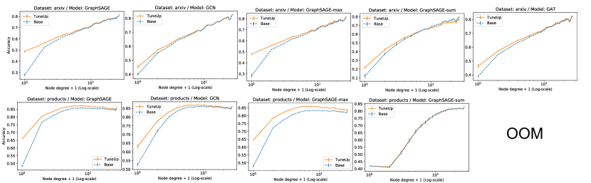
Figure 2: Degree-specific predictive performance of the base GNN and TuneUp in transductive semi-supervised node classification. The evaluation metric is classification accuracy.

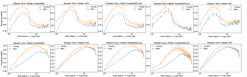
Figure 3: Degree-specific predictive performance of the base GNN and TuneUp in transductive link prediction. The evaluation metric is recall@50.

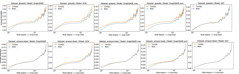
Figure 4: Degree-specific predictive performance of the base GNN and TuneUp in transductive recommender systems. The evaluation metric is recall@50.

We also analyze the degree-specific predictive improvement and highlight the results in Figure 1. The full results (the five GNN architectures times the six datasets) are available in Figures 2, 3, and 4 in Appendix. We see that TuneUp produces consistent improvement over the base GNNs across the node degrees. Not surprisingly, improvement is most significant on tail nodes.

We then focus on the two representative GNNs (GraphSAGE and GCN) and provide extensive results in Tables 3–5. Overall, TuneUp establishes its superior performance over the existing strong baseline methods by outperforming the graph augmentation methods (DropEdge and LocalAug) as well as the specialized methods for tail nodes (ColdBrew, GraphLessNN, and Tail-GNN) across the three different tasks. In particular, from the “Inductive (cold)” column, we see that TuneUp gives superior performance than ColdBrew, GraphLessNN, and Tail-GNN on the cold-start tail nodes, despite its simplicity and not requiring any loss/architectural change.

Moreover, TuneUp outperforms TuneUp w/o curriculum, which highlights the importance of the two-stage curriculum learning strategy in TuneUp. TuneUp also outperforms TuneUp w/o syn-tails and TuneUp w/o pseudo-labels, which suggests that both of the ablated components are necessary, as predicted by our theory. TuneUp is the only method that yielded consistent improvement over the base GNNs, indicating its broad applicability across the prediction tasks. More detailed discussion can be found in Appendix.

Conclusions

We presented TuneUp, a simple two-stage curriculum learning strategy for improving GNN performance, especially on tail nodes. TuneUp is simple to implement, does not require any modification to loss or model architecture, and can be used with a wide range of GNN architectures. Through extensive experiments, we demonstrated the effectiveness of TuneUp in diverse settings, including five GNN architectures, three types of prediction tasks, and three settings (transductive, inductive, and cold-start). Overall, our work suggests that even a simple training strategy can significantly improve the predictive performance of GNNs and complement parallel advances in model architectures and losses.

Appendix A Details of Datasets

Semi-supervised node classification

We used the following two datasets:

• arxiv (Hu et al. 2020): Given a paper citation network, the task is to predict the subject areas of the papers. Each paper has abstract words as its feature.

• products (Hu et al. 2020): Given a product co-purchasing network, the task is to predict the categories of the products. Each product has the product description as its feature.

Link prediction

We used the following two datasets:

• flickr (Zeng et al. 2020): Given an incomplete image-image common-property (e.g., same geographic location, same gallery, comments by the same user, etc.) network, the task is to predict the new common-property links between images. Each image has its description has its feature.

• arxiv (Hu et al. 2020): Given an incomplete paper citation network, the task is to predict the additional citation links. Each paper has words in its abstract as its feature.

Recommender systems

We used the following two datasets:

• gowalla (Liang et al. 2016; Wang et al. 2019): Given a user-location check-in bipartite graph, the task is to predict new check-in of users.

• amazon-book (He and McAuley 2016; Wang et al. 2019): Given user-product reviews, the task is to predict new reviews by users.

Appendix B Details of Hyperparameters

Here we present the details of hyperparameters we used in our experiments.

Semi-supervised node classification

We used the hidden dimensionality of 256 and 64 for arxiv and products, respectively. We trained GNNs in a full-batch manner, and for products, we used the reduced dimensionality of 64 so that the entire graph fits into the limited GPU memory of 45GB. Mini-batch training is left for future work. We used 1500 epochs for both default training and fine-tuning. The learning rate is set to 0.001.

Link prediction

We used the hidden dimensionality of 256 for all datasets. We added L2 regularization on the node embeddings and tuned its weight for each dataset and GNN architecture. For both default training and fine-tuning, we used 1000 epochs and a learning rate of 0.0001.

Recommender systems

We used the shallow embedding dimensionality of 64 and the hidden embedding dimensionality of 256. Similar to link prediction, we added L2 regularization to the node embeddings and tuned its weight for each dataset and GNN architecture. For default training, we trained the model for 2000 epochs with an initial learning rate of 0.001, which is multiplied by 0.1 at the 1000th and 1500th epoch. For fine-tuning, we used 500 epochs with a learning rate of 0.0001.

For training strategies without curriculum learning, we used the same configuration as the default training.

Appendix C Detailed Discussion on Experimental Results

Below, we provide a detailed discussion of our experimental results.

• The last rows of Tables 3, 4, and 5 highlight the relative improvement of TuneUp over the base GNNs. TuneUp improves over the base GNNs across the transductive settings, giving up to 2.0%, 57.6%, and 21.1% relative improvement in the semi-supervised node classification, link prediction, and recommender systems, respectively. Moreover, TuneUp gave even larger improvements on the challenging cold-start inductive prediction setting, yielding up to 26.2% and 92.2% relative improvement on node classification and link prediction, respectively.

• In Tables 7 and 10, we show the results of the challenging cold-start inductive prediction with the three different edge removal ratios from the new nodes. From the last rows of the tables, we see that TuneUp provides larger relative gains on larger edge removal ratios, demonstrating its high effectiveness on the highly cold-start prediction setting.

• On semi-supervised node classification (Tables 3 and 7), TuneUp w/o syn-tails gave limited performance improvement, indicating that the conventional semi-supervised training with the pseudo-labels (Lee et al. 2013) is not as effective. Moreover, TuneUp significantly outperforms TuneUp w/o pseudo-labels, especially in the inductive cold-start scenario, suggesting the benefit of pseudo-labels in increasing the supervised tail node data.

• On link prediction (Tables 4 and 10), DropEdge (TuneUp without the first stage) already gave significant performance improvement over the base GNN. This implies the unrealized potential of DropEdge on this task, beyond mitigating oversmoothing in node classification (Rong et al. 2020). Nonetheless, TuneUp still gave consistent improvement over DropEdge, suggesting the benefit of the two-stage training.

• On recommender systems (Table 5), TuneUp is the only method that produced significantly better performance than the base GNN. DropEdge and TuneUp w/o curriculum performed worse than the base GNN. This may be because jointly learning the GNN and shallow embeddings is hard without the two-stage training.

Table 6: Semi-supervised node classification performance with GCN as the backbone architecture. The evaluation metric is classification accuracy. For the “Inductive (cold),” 90% of edges are randomly removed from the new nodes. Refer to Table 8 in the Appendix for the results with different edge removal ratios.

Method	arxiv			products
	Transductive	Inductive	Inductive (cold)	Transductive	Inductive	Inductive (cold)
Base	0.6921$\pm$0.0004	0.6893$\pm$0.0021	0.5491$\pm$0.0042	0.8432$\pm$0.0007	0.8447$\pm$0.0008	0.7461$\pm$0.0033
DropEdge	0.6958$\pm$0.0007	0.6938$\pm$0.0013	0.5632$\pm$0.0019	0.8486$\pm$0.0004	0.8495$\pm$0.0008	0.7661$\pm$0.0019
LocalAug	0.6986$\pm$0.0010	0.6963$\pm$0.0022	0.5680$\pm$0.0042	0.8485$\pm$0.0005	0.8497$\pm$0.0002	0.7505$\pm$0.0025
ColdBrew	0.6862$\pm$0.0004	0.6726$\pm$0.0031	0.5376$\pm$0.0076	0.8402$\pm$0.0008	0.8412$\pm$0.0006	0.7396$\pm$0.0031
GraphLessNN	0.6129$\pm$0.0008	0.5462$\pm$0.0021	0.5462$\pm$0.0021	0.6671$\pm$0.0008	0.6649$\pm$0.0006	0.6649$\pm$0.0006
RAWLS-GCN	0.6706$\pm$0.0013	0.6696$\pm$0.0027	0.5326$\pm$0.0027	0.8210$\pm$0.0008	0.8223$\pm$0.0009	0.7113$\pm$0.0013
Tail-GNN	0.6434$\pm$0.0010	0.6402$\pm$0.0007	0.5381$\pm$0.0054	OOM	OOM	OOM
TuneUp w/o curriculum	0.6960$\pm$0.0009	0.6927$\pm$0.0023	0.5605$\pm$0.0031	0.8482$\pm$0.0006	0.8489$\pm$0.0004	0.7640$\pm$0.0023
TuneUp w/o pseudo-labels	0.6965$\pm$0.0008	0.6935$\pm$0.0015	0.5567$\pm$0.0035	0.8490$\pm$0.0007	0.8497$\pm$0.0009	0.7670$\pm$0.0036
TuneUp w/o syn-tails	0.6936$\pm$0.0006	0.6924$\pm$0.0027	0.5590$\pm$0.0053	0.8452$\pm$0.0006	0.8467$\pm$0.0006	0.7550$\pm$0.0024
TuneUp (ours)	0.6989$\pm$0.0006	0.6990$\pm$0.0019	0.5916$\pm$0.0044	0.8523$\pm$0.0007	0.8536$\pm$0.0006	0.7924$\pm$0.0050
Rel. gain over base	+1.0%	+1.4%	+7.7%	+1.1%	+1.1%	+6.2%

Table 7: Cold-start inductive node classification performance with GraphSAGE as the backbone architecture. The larger the edge removal ratio is, the more cold-start the prediction task becomes. The evaluation metric is classification accuracy. Refer to Table 8 in Appendix for the performance with GCN, where a similar trend is observed.

Method	arxiv			products
	Edge removal ratio			Edge removal ratio
	30%	60%	90%	30%	60%	90%
Base	0.6450$\pm$0.0023	0.5993$\pm$0.0013	0.4752$\pm$0.0061	0.8334$\pm$0.0008	0.8130$\pm$0.0008	0.7227$\pm$0.0011
DropEdge	0.6534$\pm$0.0017	0.6248$\pm$0.0041	0.5449$\pm$0.0059	0.8411$\pm$0.0007	0.8281$\pm$0.0005	0.7709$\pm$0.0014
LocalAug	0.6547$\pm$0.0016	0.6149$\pm$0.0011	0.4981$\pm$0.0018	0.8370$\pm$0.0006	0.8166$\pm$0.0010	0.7261$\pm$0.0008
ColdBrew	0.6283$\pm$0.0035	0.5923$\pm$0.0017	0.5082$\pm$0.0018	0.8309$\pm$0.0008	0.8134$\pm$0.0007	0.7395$\pm$0.0019
GraphLessNN	0.5456$\pm$0.0008	0.5456$\pm$0.0008	0.5456$\pm$0.0008	0.6648$\pm$0.0009	0.6648$\pm$0.0009	0.6648$\pm$0.0009
Tail-GNN	0.6389$\pm$0.0011	0.6123$\pm$0.0023	0.5388$\pm$0.0031	OOM	OOM	OOM
TuneUp w/o curriculum	0.6531$\pm$0.0023	0.6266$\pm$0.0033	0.5472$\pm$0.0119	0.8396$\pm$0.0006	0.8243$\pm$0.0007	0.7569$\pm$0.0015
TuneUp w/o pseudo-labels	0.6498$\pm$0.0030	0.6192$\pm$0.0038	0.5332$\pm$0.0077	0.8405$\pm$0.0010	0.8262$\pm$0.0016	0.7631$\pm$0.0055
TuneUp w/o syn-tails	0.6518$\pm$0.0016	0.6106$\pm$0.0025	0.4899$\pm$0.0047	0.8362$\pm$0.0004	0.8162$\pm$0.0005	0.7258$\pm$0.0011
TuneUp (ours)	0.6685$\pm$0.0022	0.6504$\pm$0.0024	0.5996$\pm$0.0012	0.8521$\pm$0.0005	0.8432$\pm$0.0005	0.8054$\pm$0.0011
Rel. gain over base	+3.6%	+8.5%	+26.2%	+2.2%	+3.7%	+11.4%

Table 8: Cold-start inductive node classification performance with GCN as the backbone architecture. The larger the edge removal ratio is, the more cold-start the prediction task becomes. The evaluation metric is classification accuracy.

Method	arxiv			products
	Edge removal ratio			Edge removal ratio
	30%	60%	90%	30%	60%	90%
Base	0.6713$\pm$0.0019	0.6401$\pm$0.0029	0.5491$\pm$0.0042	0.8375$\pm$0.0008	0.8209$\pm$0.0012	0.7461$\pm$0.0033
DropEdge	0.6756$\pm$0.0016	0.6475$\pm$0.0026	0.5632$\pm$0.0019	0.8435$\pm$0.0006	0.8298$\pm$0.0008	0.7661$\pm$0.0019
LocalAug	0.6776$\pm$0.0019	0.6489$\pm$0.0025	0.5680$\pm$0.0042	0.8423$\pm$0.0008	0.8261$\pm$0.0008	0.7505$\pm$0.0025
ColdBrew	0.6513$\pm$0.0044	0.6188$\pm$0.0047	0.5376$\pm$0.0076	0.8338$\pm$0.0008	0.8168$\pm$0.0013	0.7396$\pm$0.0031
GraphLessNN	0.5462$\pm$0.0021	0.5462$\pm$0.0021	0.5462$\pm$0.0021	0.6649$\pm$0.0006	0.6649$\pm$0.0006	0.6649$\pm$0.0006
RAWLS-GCN	0.6490$\pm$0.0016	0.6117$\pm$0.0027	0.5326$\pm$0.0027	0.8130$\pm$0.0007	0.7924$\pm$0.0006	0.7113$\pm$0.0013
Tail-GNN	0.6277$\pm$0.0012	0.6058$\pm$0.0015	0.5381$\pm$0.0054	OOM	OOM	OOM
TuneUp w/o curriculum	0.6751$\pm$0.0017	0.6453$\pm$0.0021	0.5605$\pm$0.0031	0.8427$\pm$0.0005	0.8288$\pm$0.0004	0.7640$\pm$0.0023
TuneUp w/o pseudo-labels	0.6751$\pm$0.0027	0.6451$\pm$0.0030	0.5567$\pm$0.0035	0.8439$\pm$0.0011	0.8299$\pm$0.0013	0.7670$\pm$0.0036
TuneUp w/o syn-tails	0.6737$\pm$0.0015	0.6469$\pm$0.0022	0.5590$\pm$0.0053	0.8398$\pm$0.0006	0.8247$\pm$0.0010	0.7550$\pm$0.0024
TuneUp (ours)	0.6815$\pm$0.0025	0.6606$\pm$0.0004	0.5916$\pm$0.0044	0.8489$\pm$0.0007	0.8385$\pm$0.0014	0.7924$\pm$0.0050
Rel. gain over base	+1.5%	+3.2%	+7.7%	+1.4%	+2.1%	+6.2%

Table 9: Link prediction performance with GCN as the backbone architecture. The evaluation metric is recall@50. For the “Inductive (cold),” 60% of edges are randomly removed from the new nodes. Refer to Table 11 in the Appendix for the results with different edge removal ratios.

Method	flickr			arxiv
	Transductive	Inductive	Inductive (cold)	Transductive	Inductive	Inductive (cold)
Base	0.1355$\pm$0.0007	0.1366$\pm$0.0008	0.0863$\pm$0.0009	0.2242$\pm$0.0005	0.2052$\pm$0.0005	0.1185$\pm$0.0011
DropEdge	0.1479$\pm$0.0005	0.1401$\pm$0.0014	0.1001$\pm$0.0019	0.2394$\pm$0.0014	0.2108$\pm$0.0012	0.1348$\pm$0.0013
LocalAug	0.1408$\pm$0.0011	0.1430$\pm$0.0007	0.0930$\pm$0.0009	0.2324$\pm$0.0013	0.2136$\pm$0.0020	0.1209$\pm$0.0007
ColdBrew	0.1177$\pm$0.0015	0.1174$\pm$0.0029	0.0731$\pm$0.0025	0.1978$\pm$0.0024	0.1788$\pm$0.0037	0.0967$\pm$0.0031
RAWLS-GCN	0.0660$\pm$0.0020	0.0422$\pm$0.0020	0.0406$\pm$0.0018	0.1057$\pm$0.0017	0.0814$\pm$0.0027	0.0409$\pm$0.0017
Tail-GNN	0.1287$\pm$0.0017	0.1292$\pm$0.0020	0.0872$\pm$0.0017	0.1492$\pm$0.0012	0.1336$\pm$0.0022	0.0812$\pm$0.0022
TuneUp w/o curriculum	0.1486$\pm$0.0009	0.1434$\pm$0.0024	0.1027$\pm$0.0015	0.2401$\pm$0.0022	0.2121$\pm$0.0023	0.1328$\pm$0.0008
TuneUp w/o syn-tails	0.1395$\pm$0.0022	0.1408$\pm$0.0024	0.0899$\pm$0.0020	0.2282$\pm$0.0026	0.2096$\pm$0.0032	0.1181$\pm$0.0011
TuneUp (ours)	0.1577$\pm$0.0011	0.1510$\pm$0.0016	0.1072$\pm$0.0011	0.2527$\pm$0.0017	0.2239$\pm$0.0027	0.1428$\pm$0.0021
Rel. gain over base	+16.4%	+10.6%	+24.2%	+12.7%	+9.1%	+20.5%

Table 10: Cold-start inductive link prediction performance with GraphSAGE. The evaluation metric is recall@50. The larger the edge removal ratio is, the more cold-start the prediction task becomes. Refer to Table 11 in Appendix for the performance with GCN, where a similar trend is observed.

Method	flickr			arxiv
	Edge removal ratio			Edge removal ratio
	30%	60%	90%	30%	60%	90%
Base	0.0809$\pm$0.0013	0.0582$\pm$0.0014	0.0173$\pm$0.0038	0.0990$\pm$0.0032	0.0688$\pm$0.0020	0.0208$\pm$0.0011
DropEdge	0.1136$\pm$0.0013	0.0992$\pm$0.0008	0.0594$\pm$0.0012	0.1529$\pm$0.0036	0.1189$\pm$0.0046	0.0570$\pm$0.0034
LocalAug	0.0899$\pm$0.0051	0.0646$\pm$0.0059	0.0250$\pm$0.0159	0.1038$\pm$0.0042	0.0734$\pm$0.0036	0.0266$\pm$0.0062
ColdBrew	0.0547$\pm$0.0057	0.0369$\pm$0.0045	0.0266$\pm$0.0057	0.0898$\pm$0.0035	0.0640$\pm$0.0031	0.0331$\pm$0.0027
Tail-GNN	0.0663$\pm$0.0018	0.0657$\pm$0.0016	0.0529$\pm$0.0075	0.0725$\pm$0.0031	0.0586$\pm$0.0031	0.0371$\pm$0.0036
TuneUp w/o curriculum	0.1184$\pm$0.0020	0.1014$\pm$0.0018	0.0622$\pm$0.0020	0.1488$\pm$0.0049	0.1144$\pm$0.0041	0.0535$\pm$0.0045
TuneUp w/o syn-tails	0.0800$\pm$0.0022	0.0583$\pm$0.0013	0.0173$\pm$0.0038	0.1017$\pm$0.0032	0.0728$\pm$0.0032	0.0301$\pm$0.0099
TuneUp (ours)	0.1259$\pm$0.0051	0.1119$\pm$0.0069	0.0734$\pm$0.0084	0.1574$\pm$0.0021	0.1241$\pm$0.0025	0.0598$\pm$0.0028
Rel. gain over base	+55.6%	+92.2%	+324.3%	+59.0%	+80.4%	+187.5%

Table 11: Cold-start inductive link prediction performance with GCN. The evaluation metric is recall@50. The larger the edge removal ratio is, the more cold-start the prediction task becomes.

Method	flickr			arxiv
	Edge removal ratio			Edge removal ratio
	30%	60%	90%	30%	60%	90%
Base	0.1137$\pm$0.0012	0.0863$\pm$0.0009	0.0256$\pm$0.0006	0.1701$\pm$0.0009	0.1185$\pm$0.0011	0.0381$\pm$0.0006
DropEdge	0.1224$\pm$0.0014	0.1001$\pm$0.0019	0.0620$\pm$0.0031	0.1816$\pm$0.0010	0.1348$\pm$0.0013	0.0591$\pm$0.0016
LocalAug	0.1192$\pm$0.0012	0.0930$\pm$0.0009	0.0298$\pm$0.0023	0.1763$\pm$0.0016	0.1209$\pm$0.0007	0.0366$\pm$0.0012
ColdBrew	0.0948$\pm$0.0032	0.0731$\pm$0.0025	0.0542$\pm$0.0019	0.1458$\pm$0.0031	0.0967$\pm$0.0031	0.0383$\pm$0.0045
RAWLS-GCN	0.0404$\pm$0.0021	0.0406$\pm$0.0018	0.0397$\pm$0.0014	0.0625$\pm$0.0019	0.0409$\pm$0.0017	0.0247$\pm$0.0019
Tail-GNN	0.1093$\pm$0.0016	0.0872$\pm$0.0017	0.0511$\pm$0.0029	0.1123$\pm$0.0023	0.0812$\pm$0.0022	0.0421$\pm$0.0041
TuneUp w/o curriculum	0.1240$\pm$0.0023	0.1027$\pm$0.0015	0.0638$\pm$0.0014	0.1812$\pm$0.0014	0.1328$\pm$0.0008	0.0547$\pm$0.0037
TuneUp w/o syn-tails	0.1186$\pm$0.0025	0.0899$\pm$0.0020	0.0274$\pm$0.0029	0.1716$\pm$0.0019	0.1181$\pm$0.0011	0.0357$\pm$0.0018
TuneUp (ours)	0.1292$\pm$0.0013	0.1072$\pm$0.0011	0.0677$\pm$0.0030	0.1920$\pm$0.0020	0.1428$\pm$0.0021	0.0610$\pm$0.0026
Rel. gain over base	+13.7%	+24.2%	+164.1%	+12.9%	+20.5%	+60.3%

Appendix D Theoretical Analysis

Technical Details

The generalization improvement on low-degree nodes is expected to happen when the label distribution for each node is invariant w.r.t. the degree of nodes. This condition is captured by the following generating process for the considered part of a graph. A finite set $\mathcal{Z}$ of (arbitrarily) large size that consists of $(x,y)$ pairs are sampled accordingly to some unknown distribution without graph structure first. Then, $(\bar{x}_{i},\bar{y}_{i})_{i=1}^{T}$ and $(\tilde{x}_{i},\tilde{y}_{i})_{i=1}^{R}$ are sampled uniformly from $\mathcal{Z}$ without replacement, where $(\bar{x}_{i},\bar{y}_{i})_{i=1}^{T}$ and $(\tilde{x}_{i},\tilde{y}_{i})_{i=1}^{R}$ are used in the zero degree nodes and the full degree nodes in the part of a graph $G$, respectively. Define $A$ and $B$ to be the sets of node indices of the zero degree and the full degrees, respectively. The labeled node indices for the full degree are sampled uniformly from $B$ and its set is denoted by $S=\{i\in B:i\text{-th node is in the labeled training dataset}\}$. Let $\theta$ be the parameter trained with a set of labeled nodes $S$. We use nodes $A$ as test data.

We consider a $K$-layer GNN of a standard form: $f(X)=H_{K}\in\mathbb{R}^{n}$ with $H_{k}=\sigma_{k}(JH_{k-1}W_{k}+1_{n}b_{k})$, where $n$ is the number of all nodes, $\sigma_{K}=\mathop{\mathrm{sign}}$, $\sigma_{k}$ represents the ReLU nonlinear function for $k\neq K$, $1_{n}$ is the column vector of size $n$ with all entries being ones, $(W_{k},b_{k})$ are the learnable parameters included in $\theta$, $H_{0}=X$, $W_{K}\in\mathbb{R}^{d\times 1}$, and $b_{K}\in\mathbb{R}$. Here, $J\in\mathbb{R}^{n\times n}$ is defined by $J=\mathbf{A}+\mathbf{I},$ where $\mathbf{A}\in\mathbb{R}^{n\times n}$ denotes the graph adjacency matrix and $\mathbf{I}\in\mathbb{R}^{n\times n}$ is the identity matrix.

Define $\ell(i)$ and $\mathcal{L}(i)$ to be the 0-1 losses of $i$-th node with and without dropping edges: i.e., $\ell(i)$ is the 0-1 loss of $i$-th node with the model $F_{\theta}(\widetilde{G})$ using the modified graph $\widetilde{G}$ that drops all edges for $i\in B$, whereas $\mathcal{L}(i)$ is the loss with the original graph. Define $\tilde{\ell}$ by $\tilde{\ell}(i)=\ell(i)$ for $i\in S$ and $\tilde{\ell}(i)$ is the loss with the pseudo label for $i\in B\setminus S$. The function $\tilde{\mathcal{L}}$ is defined similarly for $\mathcal{L}$ with the pseudo label but without dropping edges. Define the average training loss at the end of the 1st stage of the curriculum-based training by $Q=\frac{1}{|S|}\sum_{t\in S}\mathcal{L}_{1}(t),$ where $\mathcal{L}_{1}(i)$ is the 0-1 loss of $i$-th node at the end of the 1st stage. For methods $M_{1}$–$M_{3}$, we define the generalization gap between the test errors of nodes with low degrees and the training errors of nodes with high degrees by $\Delta(M_{1})=\frac{1}{|A|}\sum_{i\in A}\mathcal{L}(i)-\frac{1}{|S|}\sum_{i\in S}\ell(i)$, $\Delta(M_{2})=\frac{1}{|A|}\sum_{i\in A}\mathcal{L}(i)-\frac{1}{|B|}\sum_{i\in B}\tilde{\ell}(i)$, $\Delta(M_{3})=\frac{1}{|A|}\sum_{i\in A}\mathcal{L}(i)-\frac{1}{|B|}\sum_{i\in B}\tilde{\mathcal{L}}(i)$.

Theorem 2 (A more detailed version of Theorem 1).

For any $\delta>0$, with probability at least $1-\delta$, the following holds for all $M\in\{M_{1},M_{2},M_{3}\}$:

$$\Delta(M) \leq\sqrt{\frac{\mathbf{1}\{M=M_{1}\}8(d-1)\ln(\frac{16e|S|}{\delta})+8\ln(\frac{16e|S|}{\delta})}{|S|}}+\mathbf{1}\{M\neq M_{1}\}Q+\mathbf{1}\{M=M_{3}\}\tau+G,$$

where $\tau=\frac{1}{|B|}\sum_{i\in B}\left(\ell(i)-\mathcal{L}(i)\right)$ and $G=\sqrt{\frac{8d\ln(16eR/\delta)}{R}}+\sqrt{\frac{\ln(4/\delta)}{2T}}$.

Proof of Theorem 2

Recall the following lemma from (Hoeffding 1963, Theorem 4):

Lemma 1 (Hoeffding 1963).

Let $\mathcal{X}$ be a finite population of $N$ real points, $X_{1},\dots,X_{n}$ denote a random sample without replacement drawn uniformly from $\mathcal{X}$, and $\bar{X}_{1},\dots,\bar{X}_{n}$ denote a random sample with replacement drawn uniformly from $\mathcal{X}$. If $g:\mathbb{R}\rightarrow\mathbb{R}$ is continuous and convex,

$$\mathbb{E}\left[g\left(\sum_{i=1}^{n}X_{i}\right)\right]\leq\mathbb{E}\left[g\left(\sum_{i=1}^{n}\bar{X}_{i}\right)\right].$$

We utilize this lemma in our proof.

Proof of Theorem 2.

Without loss of generality, we order the node index such that this part of a graph with the $T$ nodes with zero degree and the $R$ nodes with full degree comes first in node index ordering: i.e., $i$-th node is in the group with zero degree for $i\in A=\{1,\dots,T\}$ and with full degree for $i\in B=\{T+1,\dots,T+R\}$. Define $\Delta_{1}=\Delta(M_{1})$ and $\Delta_{2}=\Delta(M_{2})$. Since $\frac{1}{|A|}\sum_{i\in A}\mathcal{L}(i)=\frac{1}{|A|}\sum_{i\in A}\ell(i)$,

$$\Delta_{1}=\frac{1}{|A|}\sum_{i\in A}\ell(i)-\frac{1}{|S|}\sum_{i\in S}\ell(i)$$

$$\Delta_{2}=\frac{1}{|A|}\sum_{i\in A}\ell(i)-\frac{1}{|B|}\sum_{i\in B}\tilde{\ell}(i).$$

$$\Delta_{3}=\frac{1}{|A|}\sum_{i\in A}\ell(i)-\frac{1}{|B|}\sum_{i\in B}\tilde{\mathcal{L}}(i)$$

Since $\mathcal{Z}$ is finite, we can write $\mathcal{Z}=\{z_{i}:i\in[N]\}$ where $z_{i}=(x_{i},y_{i})$ and $[N]=\{1,2,\dots,N\}$ for some (arbitrarily large) $N$. Then, $(\bar{x}_{i},\bar{y}_{i})$ and $(\tilde{x}_{i},\tilde{y}_{i})$ can be equivalently defined as follows: we define $(\bar{x}_{i},\bar{y}_{i})$ by setting its value to be $(x_{t_{i}},y_{t_{i}})$ (for $i=1\dots,T$) and define $(\tilde{x}_{i},\tilde{y}_{i})$ by setting its value to be $(x_{r_{i}},y_{r_{i}})$ for $i=1\dots,R$, where $t_{1},\dots,t_{T}$ and $r_{1},\dots,r_{R}$ are sampled sampled uniformly from $[N]$ without replacement. Define a loss function with node features and label by $\phi(\bar{z}_{i})=\ell(i)$ where $\bar{z}_{i}=(\bar{x}_{i},\bar{y}_{i})=(x_{t_{i}},y_{t_{i}})=z_{t_{i}}$ for . With this, since $\frac{1}{|A|}\sum_{i\in A}\phi(\bar{z}_{i})=\frac{1}{|A|}\sum_{i\in A}\phi(z_{t_{i}})=\frac{1}{T}\sum_{i=1}^{T}\phi(z_{t_{i}})$,

$$\Delta_{1}=\frac{1}{T}\sum_{i=1}^{T}\phi(z_{t_{i}})-\frac{1}{|S|}\sum_{i\in S}\ell(i)$$

$$\Delta_{2}=\frac{1}{T}\sum_{i=1}^{T}\phi(z_{t_{i}})-\frac{1}{|B|}\sum_{i\in B}\tilde{\ell}(i).$$

$$\Delta_{3}=\frac{1}{T}\sum_{i=1}^{T}\phi(z_{t_{i}})-\frac{1}{|B|}\sum_{i\in B}\tilde{\mathcal{L}}(i).$$

Hoeffding (1963) shows that using Lemma 1 within the proof of (standard) Hoeffding’s inequality, (standard) Hoeffding’s inequality still holds for samples without replacement. Since $\ell(i)\in[0,1]$ for all $i\in[N]$,

$$\mathbb{P}\left(\frac{1}{T}\sum_{i=1}^{T}\phi(z_{t_{i}})-\frac{1}{N}\sum_{i=1}^{N}\phi(z_{i})\geq\epsilon\right)\leq\exp\left(-2T\epsilon^{2}\right).$$

By setting $\delta=\exp\left(-2T\epsilon^{2}\right)$ and solving for $\epsilon$, this implies that for any $\delta>0$, with probability at least $1-\delta$,

$$\frac{1}{T}\sum_{i=1}^{T}\phi(z_{t_{i}})\leq\frac{1}{N}\sum_{i=1}^{N}\phi(z_{i})+\sqrt{\frac{\ln(1/\delta)}{2T}}.$$

Therefore, for any $\delta>0$, with probability at least $1-\delta$,

$$\Delta_{1}\leq\frac{1}{N}\sum_{i=1}^{N}\phi(z_{i})-\frac{1}{|S|}\sum_{i\in S}\ell(i)+\sqrt{\frac{\ln(1/\delta)}{2T}},\text{ and, }$$

$$\Delta_{2}\leq\frac{1}{N}\sum_{i=1}^{N}\phi(z_{i})-\frac{1}{|B|}\sum_{i\in B}\tilde{\ell}(i)+\sqrt{\frac{\ln(1/\delta)}{2T}}.$$

$$\Delta_{3}\leq\frac{1}{N}\sum_{i=1}^{N}\phi(z_{i})-\frac{1}{|B|}\sum_{i\in B}\tilde{\mathcal{L}}(i)+\sqrt{\frac{\ln(1/\delta)}{2T}}.$$

For $\Delta_{1}$, we have

$$\Delta_{1} \leq\frac{1}{N}\sum_{i=1}^{N}\phi(z_{i})-\frac{1}{|S|}\sum_{i\in S}\ell(i)+\sqrt{\frac{\ln(1/\delta)}{2T}}\pm\frac{1}{|B|}\sum_{i\in B}\ell(i)$$

$$=\left(\frac{1}{N}\sum_{i=1}^{N}\phi(z_{i})-\frac{1}{|B|}\sum_{i\in B}\ell(i)\right)+\left(\frac{1}{|B|}\sum_{i\in B}\ell(i)-\frac{1}{|S|}\sum_{i\in S}\ell(i)\right)+\sqrt{\frac{\ln(1/\delta)}{2T}}$$

$$=\left(\frac{1}{N}\sum_{i=1}^{N}\phi(z_{i})-\frac{1}{R}\sum_{i=1}^{R}\phi(z_{r_{i}})\right)+\left(\frac{1}{|B|}\sum_{i\in B}\ell(i)-\frac{1}{|S|}\sum_{i\in S}\ell(i)\right)+\sqrt{\frac{\ln(1/\delta)}{2T}}$$

Similarly, for $\Delta_{2}$ and $\Delta_{3}$,

$$\Delta_{2}\leq\left(\frac{1}{N}\sum_{i=1}^{N}\phi(z_{i})-\frac{1}{R}\sum_{i=1}^{R}\phi(z_{r_{i}})\right)+\left(\frac{1}{|B|}\sum_{i\in B}\ell(i)-\frac{1}{|B|}\sum_{i\in B}\tilde{\ell}(i)\right)+\sqrt{\frac{\ln(1/\delta)}{2T}}$$

$$\Delta_{3}\leq\left(\frac{1}{N}\sum_{i=1}^{N}\phi(z_{i})-\frac{1}{R}\sum_{i=1}^{R}\phi(z_{r_{i}})\right)+\left(\frac{1}{|B|}\sum_{i\in B}\ell(i)-\frac{1}{|B|}\sum_{i\in B}\tilde{\mathcal{L}}(i)\right)+\sqrt{\frac{\ln(1/\delta)}{2T}}$$

For the first term of both RHS of $\Delta_{1}$, $\Delta_{2}$, and $\Delta_{3}$, by using (Esser, Chennuru Vankadara, and Ghoshdastidar 2021, Proposition 1) with the empty graph, we have that for any $\delta>0$, with probability at least $1-\delta$,

$$\frac{1}{N}\sum_{i=1}^{N}\phi(z_{i})-\frac{1}{R}\sum_{i=1}^{R}\phi(z_{r_{i}})\leq\sqrt{\frac{8d\ln(eR)+8\ln(4/\delta)}{R}}\leq\sqrt{\frac{8d\ln(\frac{4eR}{\delta})}{R}},$$

where we have $d$ because the rank of the graph aggregation matrix for this empty graph part can be larger than $d$. For the second term of RHS of $\Delta_{1}$, similarly by using (Esser, Chennuru Vankadara, and Ghoshdastidar 2021, Proposition 1) with the empty graph, we have that for any $\delta>0$, with probability at least $1-\delta$,

$$\frac{1}{|B|}\sum_{i\in B}\ell(i)-\frac{1}{|S|}\sum_{i\in S}\ell(i)\leq\sqrt{\frac{8d\ln(e|S|)+8\ln(4/\delta)}{|S|}}\leq\sqrt{\frac{8d\ln(\frac{4e|S|}{\delta})}{|S|}}.$$

Therefore, by combining these with union bounds, we have that for any $\delta>0$, with probability at least $1-\delta$,

$$\Delta_{1}\leq\sqrt{\frac{8d\ln(\frac{12eR}{\delta})}{R}}+\sqrt{\frac{8d\ln(\frac{12e|S|}{\delta})}{|S|}}+\sqrt{\frac{\ln(3/\delta)}{2T}},\text{ and, }$$

$$\Delta_{2}\leq\sqrt{\frac{8d\ln(\frac{12eR}{\delta})}{R}}+\left(\frac{1}{|B|}\sum_{i\in B}\ell(i)-\frac{1}{|B|}\sum_{i\in B}\tilde{\ell}(i)\right)+\sqrt{\frac{\ln(3/\delta)}{2T}}.$$ (1)

$$\Delta_{3}\leq\sqrt{\frac{8d\ln(\frac{12eR}{\delta})}{R}}+\left(\frac{1}{|B|}\sum_{i\in B}\ell(i)-\frac{1}{|B|}\sum_{i\in B}\tilde{\mathcal{L}}(i)\right)+\sqrt{\frac{\ln(3/\delta)}{2T}}.$$ (2)

For the second term of RHS of $\Delta_{2}$ and $\Delta_{3}$, we formalize and take advantage of the curriculum-based training by relating this second term for the objective of the curriculum-based training and its property. That is, we formalize the fact that the generalization errors over nodes of high-degrees are minimized relatively well when compared to those of low degrees, at the first stage, because of the use of the graph structure at the first stage. Then, such low generalization errors with the full graph information is utilized to reduce the generalization errors for low degree nodes at the second stage. We formalize these intuitions in our proof.

Recall that $\tilde{\ell}(t)=\ell(t)$ for $t\in S$ and $\tilde{\ell}(t)$ is the loss with the pseudo label for $t\in B\setminus S$. Thus, we have that

$$\frac{1}{|B|}\sum_{i\in B}\ell(i)-\frac{1}{|B|}\sum_{i\in B}\tilde{\ell}(i)=\frac{1}{|B|}\sum_{i\in B}\left(\ell(i)-\tilde{\ell}(i)\right).$$

$$\frac{1}{|B|}\sum_{i\in B}\ell(i)-\frac{1}{|B|}\sum_{i\in B}\tilde{\mathcal{L}}(i)=\frac{1}{|B|}\sum_{i\in B}\left(\mathcal{L}(i)-\tilde{\mathcal{L}}(i)\right)+\frac{1}{|B|}\sum_{i\in B}\left(\ell(i)-\mathcal{L}(i)\right).$$

Here, we observe that $(\ell(i)-\tilde{\ell}(i))=0$ if the pseudo label of $i$-th node is correct. In other words, $(\ell(i)-\tilde{\ell}(i))=0$ if $\mathcal{L}_{1}(i)=0$, where $\mathcal{L}_{1}(i)$ is the 0-1 loss of $i$-th node with the model $F_{\hat{\theta}}(G)$ using the original graph $G$ where $\hat{\theta}$ is fixed at the end of the first stage of the curriculum-based training (with or without dropping edges in the second stage). Since $(\ell(i)-\tilde{\ell}(i))\leq 1$ and $\mathcal{L}_{1}(i)\in\{0,1\}$, this implies that

$$\ell(i)-\tilde{\ell}(i)\leq\mathcal{L}_{1}(i).$$

Similarly,

$$\mathcal{L}(i)-\tilde{\mathcal{L}}(i)\leq\mathcal{L}_{1}(i).$$

Combining these,

$$\Delta_{2}\leq\sqrt{\frac{8d\ln(\frac{12eR}{\delta})}{R}}+\frac{1}{|B|}\sum_{i\in B}\mathcal{L}_{1}(i)+\sqrt{\frac{\ln(3/\delta)}{2T}}$$

$$\Delta_{3}\leq\sqrt{\frac{8d\ln(\frac{12eR}{\delta})}{R}}+\frac{1}{|B|}\sum_{i\in B}\mathcal{L}_{1}(i)+\frac{1}{|B|}\sum_{i\in B}\left(\ell(i)-\mathcal{L}(i)\right)+\sqrt{\frac{\ln(3/\delta)}{2T}}$$

Here, by invoking (Esser, Chennuru Vankadara, and Ghoshdastidar 2021, Proposition 1) with the original graph $G$, we have that for any $\delta>0$, with probability at least $1-\delta$,

$$\frac{1}{|B|}\sum_{i\in B}\mathcal{L}_{1}(i)\leq\frac{1}{|S|}\sum_{t\in S}\mathcal{L}_{1}(t)+\sqrt{\frac{8\ln(\frac{4e|S|}{\delta})}{|S|}},$$

where we can remove $d$ because the rank of the graph aggregation matrix for this part of the loss is one. By combining these with equation D via union bounds, we have that for any $\delta>0$, with probability at least $1-\delta$,

$$\Delta_{1}\leq\sqrt{\frac{8d\ln(\frac{16eR}{\delta})}{R}}+\sqrt{\frac{8d\ln(\frac{16e|S|}{\delta})}{|S|}}+\sqrt{\frac{\ln(4/\delta)}{2T}},$$

$$\Delta_{2}\leq\sqrt{\frac{8d\ln(\frac{16eR}{\delta})}{R}}+\sqrt{\frac{8\ln(\frac{16e|S|}{\delta})}{|S|}}+\frac{1}{|S|}\sum_{t\in S}\mathcal{L}_{1}(t)+\sqrt{\frac{\ln(4/\delta)}{2T}},\text{ and, }$$

$$\Delta_{3}\leq\sqrt{\frac{8d\ln(\frac{16eR}{\delta})}{R}}+\sqrt{\frac{8\ln(\frac{16e|S|}{\delta})}{|S|}}+\frac{1}{|S|}\sum_{t\in S}\mathcal{L}_{1}(t)+\sqrt{\frac{\ln(4/\delta)}{2T}}+\frac{1}{|B|}\sum_{i\in B}\left(\ell(i)-\mathcal{L}(i)\right).$$

∎

References

- Bengio et al. (2009) Bengio, Y.; Louradour, J.; Collobert, R.; and Weston, J. 2009. Curriculum learning. In International Conference on Machine Learning (ICML), 41–48.
- Chen et al. (2020) Chen, M.; Wei, Z.; Huang, Z.; Ding, B.; and Li, Y. 2020. Simple and deep graph convolutional networks. In International Conference on Machine Learning (ICML), 1725–1735. PMLR.
- Clauset, Shalizi, and Newman (2009) Clauset, A.; Shalizi, C. R.; and Newman, M. E. 2009. Power-law distributions in empirical data. SIAM review, 51(4): 661–703.
- Corso et al. (2020) Corso, G.; Cavalleri, L.; Beaini, D.; Liò, P.; and Veličković, P. 2020. Principal neighbourhood aggregation for graph nets. volume 33, 13260–13271.
- Ding et al. (2022) Ding, K.; Xu, Z.; Tong, H.; and Liu, H. 2022. Data augmentation for deep graph learning: A survey. arXiv preprint arXiv:2202.08235.
- Esser, Chennuru Vankadara, and Ghoshdastidar (2021) Esser, P.; Chennuru Vankadara, L.; and Ghoshdastidar, D. 2021. Learning theory can (sometimes) explain generalisation in graph neural networks. Advances in Neural Information Processing Systems, 34: 27043–27056.
- Feng et al. (2020) Feng, W.; Zhang, J.; Dong, Y.; Han, Y.; Luan, H.; Xu, Q.; Yang, Q.; Kharlamov, E.; and Tang, J. 2020. Graph random neural networks for semi-supervised learning on graphs. Advances in Neural Information Processing Systems (NeurIPS), 33: 22092–22103.
- Fey and Lenssen (2019) Fey, M.; and Lenssen, J. E. 2019. Fast Graph Representation Learning with PyTorch Geometric. arXiv preprint arXiv:1903.02428.
- Grover and Leskovec (2016) Grover, A.; and Leskovec, J. 2016. node2vec: Scalable feature learning for networks. In ACM SIGKDD Conference on Knowledge Discovery and Data Mining (KDD), 855–864. ACM.
- Hamilton, Ying, and Leskovec (2017) Hamilton, W. L.; Ying, R.; and Leskovec, J. 2017. Inductive Representation Learning on Large Graphs. In Advances in Neural Information Processing Systems (NeurIPS), 1025–1035.
- He and McAuley (2016) He, R.; and McAuley, J. 2016. Ups and downs: Modeling the visual evolution of fashion trends with one-class collaborative filtering. In Proceedings of the International World Wide Web Conference (WWW), 507–517.
- He et al. (2020) He, X.; Deng, K.; Wang, X.; Li, Y.; Zhang, Y.; and Wang, M. 2020. Lightgcn: Simplifying and powering graph convolution network for recommendation. In ACM SIGIR conference on Research and development in Information Retrieval (SIGIR), 639–648.
- Hoeffding (1963) Hoeffding, W. 1963. Probability Inequalities for Sums of Bounded Random Variables. Journal of the American Statistical Association, 13–30.
- Hu et al. (2020) Hu, W.; Fey, M.; Zitnik, M.; Dong, Y.; Ren, H.; Liu, B.; Catasta, M.; and Leskovec, J. 2020. Open graph benchmark: Datasets for machine learning on graphs. In Advances in Neural Information Processing Systems (NeurIPS).
- Huang et al. (2021a) Huang, Q.; He, H.; Singh, A.; Lim, S.-N.; and Benson, A. R. 2021a. Combining label propagation and simple models out-performs graph neural networks.
- Huang et al. (2021b) Huang, T.; Dong, Y.; Ding, M.; Yang, Z.; Feng, W.; Wang, X.; and Tang, J. 2021b. Mixgcf: An improved training method for graph neural network-based recommender systems. In Proceedings of the 27th ACM SIGKDD Conference on Knowledge Discovery & Data Mining, 665–674.
- Kang et al. (2022) Kang, J.; Zhu, Y.; Xia, Y.; Luo, J.; and Tong, H. 2022. Rawlsgcn: Towards rawlsian difference principle on graph convolutional network. In Proceedings of the International World Wide Web Conference (WWW), 1214–1225.
- Kingma and Ba (2015) Kingma, D. P.; and Ba, J. 2015. Adam: A method for stochastic optimization. In International Conference on Learning Representations (ICLR).
- Kipf and Welling (2016) Kipf, T. N.; and Welling, M. 2016. Variational graph auto-encoders. arXiv preprint arXiv:1611.07308.
- Kipf and Welling (2017) Kipf, T. N.; and Welling, M. 2017. Semi-Supervised Classification with Graph Convolutional Networks. In International Conference on Learning Representations (ICLR).
- Klicpera, Bojchevski, and Günnemann (2019) Klicpera, J.; Bojchevski, A.; and Günnemann, S. 2019. Predict then propagate: Graph neural networks meet personalized pagerank. In International Conference on Learning Representations (ICLR).
- Kong et al. (2020) Kong, K.; Li, G.; Ding, M.; Wu, Z.; Zhu, C.; Ghanem, B.; Taylor, G.; and Goldstein, T. 2020. Flag: Adversarial data augmentation for graph neural networks. arXiv preprint arXiv:2010.09891.
- Krichene and Rendle (2020) Krichene, W.; and Rendle, S. 2020. On sampled metrics for item recommendation. In ACM SIGKDD Conference on Knowledge Discovery and Data Mining (KDD), 1748–1757.
- Lee et al. (2013) Lee, D.-H.; et al. 2013. Pseudo-label: The simple and efficient semi-supervised learning method for deep neural networks. In Workshop on challenges in representation learning, ICML, volume 3, 896.
- Li et al. (2021) Li, G.; Müller, M.; Ghanem, B.; and Koltun, V. 2021. Training graph neural networks with 1000 layers. In International Conference on Machine Learning (ICML), 6437–6449. PMLR.
- Li et al. (2019) Li, G.; Muller, M.; Thabet, A.; and Ghanem, B. 2019. Deepgcns: Can gcns go as deep as cnns? In IEEE Conference on Computer Vision and Pattern Recognition (CVPR), 9267–9276.
- Li, Han, and Wu (2018) Li, Q.; Han, Z.; and Wu, X.-M. 2018. Deeper Insights into Graph Convolutional Networks for Semi-Supervised Learning. arXiv preprint arXiv:1801.07606.
- Liang et al. (2016) Liang, D.; Charlin, L.; McInerney, J.; and Blei, D. M. 2016. Modeling user exposure in recommendation. In Proceedings of the International World Wide Web Conference (WWW), 951–961.
- Lika, Kolomvatsos, and Hadjiefthymiades (2014) Lika, B.; Kolomvatsos, K.; and Hadjiefthymiades, S. 2014. Facing the cold start problem in recommender systems. Expert systems with applications, 41(4): 2065–2073.
- Liu et al. (2022) Liu, S.; Ying, R.; Dong, H.; Li, L.; Xu, T.; Rong, Y.; Zhao, P.; Huang, J.; and Wu, D. 2022. Local augmentation for graph neural networks. In International Conference on Machine Learning (ICML), 14054–14072. PMLR.
- Liu, Nguyen, and Fang (2021) Liu, Z.; Nguyen, T.-K.; and Fang, Y. 2021. Tail-gnn: Tail-node graph neural networks. In ACM SIGKDD Conference on Knowledge Discovery and Data Mining (KDD), 1109–1119.
- Paszke et al. (2019) Paszke, A.; Gross, S.; Massa, F.; Lerer, A.; Bradbury, J.; Chanan, G.; Killeen, T.; Lin, Z.; Gimelshein, N.; Antiga, L.; et al. 2019. PyTorch: An imperative style, high-performance deep learning library. In Advances in Neural Information Processing Systems (NeurIPS), 8024–8035.
- Rendle et al. (2012) Rendle, S.; Freudenthaler, C.; Gantner, Z.; and Schmidt-Thieme, L. 2012. BPR: Bayesian personalized ranking from implicit feedback. arXiv preprint arXiv:1205.2618.
- Rong et al. (2020) Rong, Y.; Huang, W.; Xu, T.; and Huang, J. 2020. DropEdge: Towards Deep Graph Convolutional Networks on Node Classification. In International Conference on Learning Representations (ICLR).
- Rossi et al. (2020) Rossi, E.; Frasca, F.; Chamberlain, B.; Eynard, D.; Bronstein, M.; and Monti, F. 2020. SIGN: Scalable Inception Graph Neural Networks. arXiv preprint arXiv:2004.11198.
- Shi et al. (2020) Shi, Y.; Huang, Z.; Wang, W.; Zhong, H.; Feng, S.; and Sun, Y. 2020. Masked label prediction: Unified message passing model for semi-supervised classification. arXiv preprint arXiv:2009.03509.
- Shi et al. (2021) Shi, Y.; Team, P.; Huang, Z.; Li, W.; Su, W.; and Feng, S. 2021. RUnimp: SOLUTION FOR KDDCUP 2021 MAG240M-LSC.
- Velickovic et al. (2018) Velickovic, P.; Cucurull, G.; Casanova, A.; Romero, A.; Lio, P.; and Bengio, Y. 2018. Graph Attention Networks. In International Conference on Learning Representations (ICLR).
- Verma et al. (2021) Verma, V.; Qu, M.; Kawaguchi, K.; Lamb, A.; Bengio, Y.; Kannala, J.; and Tang, J. 2021. Graphmix: Improved training of gnns for semi-supervised learning. In AAAI Conference on Artificial Intelligence, volume 35, 10024–10032.
- Wang et al. (2019) Wang, X.; He, X.; Wang, M.; Feng, F.; and Chua, T.-S. 2019. Neural graph collaborative filtering. In ACM SIGIR conference on Research and development in Information Retrieval (SIGIR), 165–174.
- Wu et al. (2019) Wu, F.; Zhang, T.; Souza Jr, A. H. d.; Fifty, C.; Yu, T.; and Weinberger, K. Q. 2019. Simplifying graph convolutional networks. In International Conference on Machine Learning (ICML).
- Xu et al. (2019) Xu, K.; Hu, W.; Leskovec, J.; and Jegelka, S. 2019. How Powerful are Graph Neural Networks? In International Conference on Learning Representations (ICLR).
- Xu et al. (2018) Xu, K.; Li, C.; Tian, Y.; Sonobe, T.; Kawarabayashi, K.-i.; and Jegelka, S. 2018. Representation Learning on Graphs with Jumping Knowledge Networks. In International Conference on Machine Learning (ICML), 5453–5462.
- Ying et al. (2018) Ying, R.; He, R.; Chen, K.; Eksombatchai, P.; Hamilton, W. L.; and Leskovec, J. 2018. Graph Convolutional Neural Networks for Web-Scale Recommender Systems. In ACM SIGKDD Conference on Knowledge Discovery and Data Mining (KDD), 974–983.
- You et al. (2021) You, J.; Gomes-Selman, J. M.; Ying, R.; and Leskovec, J. 2021. Identity-aware graph neural networks. In AAAI Conference on Artificial Intelligence, volume 35, 10737–10745.
- You, Ying, and Leskovec (2020) You, J.; Ying, Z.; and Leskovec, J. 2020. Design space for graph neural networks. volume 33, 17009–17021.
- You et al. (2020) You, Y.; Chen, T.; Sui, Y.; Chen, T.; Wang, Z.; and Shen, Y. 2020. Graph contrastive learning with augmentations. Advances in Neural Information Processing Systems (NeurIPS), 33: 5812–5823.
- Zeng et al. (2020) Zeng, H.; Zhou, H.; Srivastava, A.; Kannan, R.; and Prasanna, V. 2020. GraphSaint: Graph sampling based inductive learning method. In International Conference on Learning Representations (ICLR).
- Zhang and Chen (2018) Zhang, M.; and Chen, Y. 2018. Link prediction based on graph neural networks. In Advances in Neural Information Processing Systems (NeurIPS), 5165–5175.
- Zhang et al. (2022) Zhang, S.; Liu, Y.; Sun, Y.; and Shah, N. 2022. Graph-less neural networks: Teaching old mlps new tricks via distillation. In International Conference on Learning Representations (ICLR).
- Zhao and Akoglu (2019) Zhao, L.; and Akoglu, L. 2019. Pairnorm: Tackling oversmoothing in gnns.
- Zhao et al. (2021) Zhao, T.; Liu, Y.; Neves, L.; Woodford, O.; Jiang, M.; and Shah, N. 2021. Data augmentation for graph neural networks. In AAAI Conference on Artificial Intelligence, volume 35, 11015–11023.
- Zheng et al. (2022) Zheng, W.; Huang, E. W.; Rao, N.; Katariya, S.; Wang, Z.; and Subbian, K. 2022. Cold brew: Distilling graph node representations with incomplete or missing neighborhoods. In International Conference on Learning Representations (ICLR).