A Nonlinear Sum of Squares Search for CAZAC Sequences

Abstract

We report on a search for CAZAC sequences by using nonlinear sum of squares optimization. Up to equivalence, we found all length 7 CAZAC sequences. We obtained evidence suggesting there are finitely many length 10 CAZAC sequences with a total of 3040 sequences. Last, we compute longer sequences and compare their aperiodic autocorrelation properties to known sequences. The code and results of this search are publicly available through GitHub.

I Introduction

Given $x\in\mathbb{C}^{n}$, we define the periodic ambiguity function by

$$A_{p}(x)[k,\ell]:=\frac{1}{n}\sum_{j=0}^{n-1}x_{j+k}\overline{x_{j}}e^{-2\pi ij\ell/n},$$ (1)

where $0\leq k,\ell\leq n-1$, and indices are taken modulo $n$. The periodic autocorrelation is the case with no frequency shift, i.e. when $\ell=0$. In this case it is convenient to suppress the second input and write

$$A_{p}(x)[k]:=A_{p}(x)[k,0]=\frac{1}{n}\sum_{j=0}^{n-1}x_{j+k}\overline{x_{j}}.$$ (2)

A CAZAC sequence of length $n$ as a vector $x\in\mathbb{C}^{n}$ with the properties

• $|x_{j}|=1$ for $1\leq j\leq n$,

• $A_{p}(x)[k]=0$ for $1\leq k\leq n-1$.

The first property is known as the constant amplitude property and the second is known as the zero autocorrelation property, which gives rise to the acronym CAZAC.

These sequences have several interpretations and applications which motivate their study. In communication theory they have been used to reduce the cross-correlation of signals, for uplink synchronization [9], and OFDM for 5G communication [7][15]. It is also studied as an idealized waveform with regards to the narrowband ambiguity function in radar [14]. In general, the constant amplitude allows one to encode information purely in terms of phase and the zero autocorrelation ensures no interference with shifted copies of the signal. CAZAC sequences are also known as perfect polyphase sequences and are also well studied under that name [11][12][13].

CAZAC sequences have perfect periodic autocorrelation, but many applications require their aperiodic autocorrelation. The aperiodic ambiguity function of a sequence $x\in\mathbb{C}^{n}$ is given by

$$A_{a}(x)[k,\ell]:=\sum_{j=1}^{n-1}x^{(a)}_{j+k}\overline{x^{(a)}_{j}}e^{-2\pi ij\ell/n},$$ (3)

where $0\leq k,\ell\leq n-1$ and $x^{(a)}_{j}$ is defined by

$$x_{j}^{(a)}=\begin{cases}x_{j},&\text{ if }0\leq j\leq n-1,\\ 0,&\text{ otherwise}.\end{cases}$$ (4)

The key difference is instead of taking indices modulo $n$, we set the value to zero when the index falls outside of the usual range. The aperiodic autocorrelation corresponds to $\ell=0$ and it is convenient to write

$$A_{a}(x)[k]:=A_{a}[k,0]=\sum_{j=1}^{n-1}x^{(a)}_{j+k}\overline{x^{(a)}_{j}}.$$ (5)

In particular, we use aperiodic autocorrelation to study two properties of interest. We define the peak sidelobe level (PSL) of $x\in\mathbb{C}^{n}$ by

$$\mathrm{PSL}(x)=\frac{1}{|A_{a}(x)[k]|}\max_{k\neq 0}|A_{a}[k]|,$$ (6)

and the integrated sidelobe level (ISL) by

$$\mathrm{ISL}(x)=\frac{1}{|A_{a}(x)[k]|^{2}}\sum_{k=1}^{n-1}|A_{a}[k]|^{2}.$$ (7)

Although CAZAC sequences are well studied, many things about them are still unknown. Given two CAZAC sequences, $x$ and $y$, we say they are equivalent if there exists a complex scalar $c$ with $|c|=1$ so that $y=cx$ and make the representative of the equivalence class the sequence whose first entry is 1. With this in mind, it is natural to ask: For each $n$, how many CAZAC sequences of length $n$ are there? As a partial answer, it is known that if $n$ is prime, then there are at most $\binom{2n-2}{n-1}$ CAZAC sequences [8]. If $n$ is composite and divisible by a perfect square, then there are infinitely many sequences [6][10]. If $n$ is composite and not divisible by any perfect square, then it is unknown how many there are. A brute force calculation verifies that there are finitely many for $n=6$ [5]. Beyond that, it is currently unknown.

There are additional transformations under which CAZAC sequences are closed [3]. They are a finite set of transformations so it does not fundamentally change the question of whether the set of CAZAC sequences of a given length is finite. We use these to filter out known length 7 CAZAC sequences.

Proposition 1.

Let $x\in\mathbb{C}^{n}$ be a CAZAC sequence and let $\omega=e^{2\pi i/n}$. Then, the following sequences are also CAZAC sequences:

• $(T_{k}x)_{j}=x_{j+k}$, $0\leq k\leq n-1$,

• $(M_{\ell}x)_{j}=\omega^{\ell j}x_{j}$, $0\leq\ell\leq n-1$,

• $(D_{m}x)_{j}=x_{mj},\mathrm{gcd}(m,n)=1,$

• $(\overline{x})_{j}=\overline{x_{j}}$.

II CAZAC Sequneces of Length 7

The CAZAC sequences of length 7 can be split into quadratic phase sequences and non-quadratic phase sequences. Suppose $x\in\mathbb{C}^{n}$ is defined by

$$x_{j}=e^{\pi ip(j)/n},$$

where $p(j)$ is a quadratic polynomial. In this case, we say that $x$ is a quadratic phase sequence. The polynomials associated with the known quadratic phase CAZAC sequences are

Zadoff-Chu: $$p(j)=j(j-1),\hskip 5.0pt(n\text{ odd})$$

P4: $$p(j)=j(j-n).$$

Wiener: $$p(j)=2kj^{2},\hskip 5.0pt(\mathrm{gcd}(k,n)=1,n\text{ odd}),$$

$$p(j)=kj^{2},\hskip 5.0pt(\mathrm{gcd}(k,2n)=1,n\text{ even}).$$

When $n$ is prime, there are at least $n(n-1)$ CAZAC sequences comprised of roots of unity, including the quadratic phase sequences [2]. When $n=7$, this gives at least 42 roots of unity sequences. Moreover, the transformations described in Proposition 1 will keep the sequence a root of unity sequence. On the other hand, in [4] Björck constructed CAZAC sequences comprised of non roots of unity for each prime $p>5$. The construction is as follows.

Given an odd prime $p$, let $\left(\frac{j}{p}\right)$ denote the Legendre symbol defined by

$$\left(\frac{j}{p}\right)=\begin{cases}0,&\!\!\!\!\text{ if }j\equiv 0\mod p,\\ 1,&\!\!\!\!\text{ if }j\equiv x^{2}\!\!\!\!\!\mod p,\text{ for some }x\neq 0,\\ -1,&\!\!\!\!\text{ if }j\not\equiv x^{2}\mod p,\text{ for any }x\neq 0.\end{cases}$$

We define the Björck sequence of length $p$ by

$$x_{j}=e^{i\theta(j)},\hskip 5.0pt0\leq j\leq p-1,$$ (8)

where if $p\equiv 1\mod 4$, then $\theta(j)$ is given by

$$\left(\frac{j}{p}\right)\mathrm{arccos}\left(\frac{1}{1+\sqrt{p}}\right),$$ (9)

and if $p\equiv 3\mod 4$, then $\theta(j)$ is given by

$$\theta(j)=\begin{cases}\mathrm{arccos}\left(\frac{1-p}{1+p}\right)&\text{ if }\left(\frac{j}{p}\right)=-1,\\ 0,&\text{ otherwise}.\end{cases}$$ (10)

Since $7\equiv 3\mod 4$, the Björck sequence of length 7 is

$$x=(1,1,1,e^{i\theta_{7}},1,e^{i\theta_{7}},e^{i\theta_{7}}),$$ (11)

where $\theta_{7}=\mathrm{arccos}(3/4)$. Since CAZAC sequences are closed under the operations outlined in Proposition 1 the Björck sequence generates up to 252 CAZAC sequences which begin with 1 when p = 7. Some combinations of transformations result in the same sequence and thus this is an over count, which our computations reflect. Regardless, a total of at most 294 of the 532 sequences are accounted for, leaving many new sequences of length 7 to be found.

III CAZACs as an Algebraic Variety

The conditions which define a CAZAC sequence can be viewed as a system of $2n-1$ equations with $n$ variables. A natural question is to ask about the dimension of the set of solutions to this system. If the set of solutions is zero dimensional, then it is a discrete set and may be a finite set. Conversely, if the set of solutions has positive dimension, then there are infinitely many of them. This question puts the problem in the realm of algebraic geometry.

The techniques of algebraic geometry only work with systems of polynomials. However, the conjugations in the sums prevent those conditions from being interpreted as polynomials. We can get around this by expressing entries in real and imaginary parts and converting the equations to polynomials of real variables. Given a vector $X\in\mathbb{C}^{n}$ and expressing its entries as $x_{j}=a_{j}+ib_{j}$, CAZAC sequences arise as solutions to the system

$$a_{j}^{2}+b_{j}^{2}=1, \hskip 10.00002pt0\leq j\leq n-1,$$ (12)

$$\sum_{j=0}^{n-1}a_{j+k}a_{j}+b_{j+k}b_{j}=0, \hskip 10.00002pt1\leq k\leq n-1,$$ (13)

$$\sum_{j=0}^{n-1}a_{j}b_{j+k}-b_{j}a_{j+k}=0, \hskip 10.00002pt1\leq k\leq n-1.$$ (14)

Since constraining each amplitude has $n$ conditions, and each of the $n-1$ autocorrelation conditions has been split into real and imaginary parts, there are $3n-2$ equations in this system. Since each entry of the sequence was split into a real and imaginary part, the system has $2n$ variables. Hence, the system is a real algebraic variety with $3n-2$ equations and $2n$ variables.

IV Nonlinear Least Squares Search

The system of equations (12) - (14) can be converted into an unconstrained nonlinear sum of squares optimization problem. Let $a=(a_{1},\cdots,a_{n})$ and $b=(b_{1},\cdots,b_{n})$, and for each $1\leq k\leq n-1$ and $0\leq\ell\leq n-1$, define the functions

$$f_{\ell}(a,b) =a_{\ell}^{2}+b_{\ell}^{2}-1,$$ (15)

$$g_{k}(a,b) =\sum_{j=0}^{n-1}a_{j+k}a_{j}+b_{j+k}b_{j},$$ (16)

$$h_{k}(a,b) =\sum_{j=0}^{n-1}a_{j}b_{j+k}-b_{j}a_{j+k}.$$ (17)

Note that $(a,b)$ are the real and imaginary parts, respectively, of a CAZAC sequence precisely when all $3n-2$ functions are all zero at $(a,b)$. We can obtain CAZAC sequences as solutions to the unconstrained optimization problem

$$\operatorname*{arg\,min}_{(a,b)}\sum_{\ell=0}^{n-1}f_{\ell}^{2}+\sum_{k=1}^{n-1}g_{k}^{2}+h_{k}^{2},$$ (18)

for which the objective function is zero.

Since the equations are nonlinear polynomials, optimization procedures are not guaranteed to work. Specifically, there may be local minima where the objective function is greater than zero. Moreover, the objective function is not convex which makes it difficult to give theoretical guarantees about this method. Nonetheless, in our experiments we found very few such local minima and generated as many sequences as needed for each test.

V Method

The experimental design was implemented in a Jupyter Notebook. All trials were run on a 2020 MacBook Pro with the 10-core M1 Pro CPU and 16 GB of physical memory. The optimization problem in (18) was implemented using the least squares solver in SciPy’s Optimization package. By default the solver uses the Trust Region Reflective (TRR) algorithm and a finite difference operation to estimate the Jacobian at each point. The code is available through GitHub at: https://github.com/magsino-usna/IEEE-SoS-CAZAC.git.

V-A Length 7 CAZACS

We perform the optimization on 10,000 random initial starting points in $[-1,1]^{14}$. For increased precision, we used stronger tolerances of $10^{-12}$ instead of the default $10^{-8}$ for changes in the gradient, input variables, and cost function. If the resulting cost function was lower than $10^{-10}$, we considered the point found as a CAZAC sequence stored it as a new row in an array.

After generating the list of sequences, we rounded each one to 8 decimal places and pass the rounded list through NumPy’s algorithm for determining unique rows in arrays to determine the number of sequences found. After that, we used the transformations listed in Proposition 1 using the Björck and the Wiener sequences as base sequences to filter out all previously known CAZAC sequences.

V-B Length 10 CAZACs

Since 10 is composite and not divisible by a perfect square, it is not known if there are finitely many of them. Our idea for exploring whether the set of solutions is finite is based on the following intuition.

Solving the sum of squares minimization with an initial point is essentially projecting the point onto the set of solutions. If the set of solutions is greater than zero dimensional, most of the initialization points will project to different points on the continuous set of solutions. Conversely, if the set of solutions is zero dimensional and finite, then most of the points should project to that finite set of points. Thus, if the number of unique sequences found is far smaller than the number of trials, the set is likely finite. This idea is illustrated in Fig. 1.

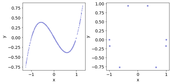
Figure 1: Experiments taking 1000 initial points and using nonlinear sum-of-squares to find points onto two sets. Left: The points traced out the one dimensional curve $x^{3}-x-y=0$. Right: The points went to the 8 points of the intersection of $x^{2}+y^{2}-1=0$ and $8x^{4}-10x^{2}-x+2=0$.

For the experiment, we performed the optimization on 200,000 random initial starting points in $[-1,1]^{20}$ and use the same tolerances and rounding method as in the length 7 case.

V-C Aperiodic Autocorrelations of Longer CAZACs

Using the nonlinear sum of squares optimization method, we computed 1000 CAZAC sequences of prime lengths $n=11,13,17,23,29,37,43,47$. We then compared the PSL and ISL of the CAZAC sequences to the PSL and ISL of the corresponding Zadoff-Chu and Björck sequences. We compare the results using a box plot to give a sense of how generic CAZAC sequences behave with respect to PSL and ISL behavior.

VI Results

As previously mentioned, all results and code are stored on GitHub: The full list is available on GitHub: https://github.com/magsino-usna/IEEE-SoS-CAZAC.git.

VI-A Length 7 Sequences

We were able to enumerate all 532 CAZAC, handling equivalence by dividing and making the first entry 1. This took 15 min to run all 100,000 attempts on the aforementioned MacBook Pro. The maximum final value of the objective function across all trials was on the order of $10^{-17}$ which implies the objective function has no spurious local minima in the length 7 case. We picked out the new CAZAC with the best PSL and compared its autocorrelation to the Zadoff-Chu and Björck sequences in Fig. 2.

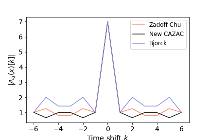
Figure 2: Autocorrelation of the best performing length 7 CAZAC sequence plotted against the autocorrelations of the length 7 Zadoff-Chu and Björck sequences. The new CAZAC sequence achieves a lower PSL than the Zadoff-Chu sequence.

VI-B Length 10 Sequences

We ran three sets of the trials described in Section V-B. In all three trials, the same 3040 CAZAC sequences were found. This heavily implies that there are 3040 CAZAC sequences of length 10, although it is still possible that points corresponding to a highly unstable minimum could be missed. However, the average runtime for each set of these trials was about 13 hours. The maximum cost function value across all trials was to the order of $10^{-24}$, which implies once again that every local minimum of the objective function is the global minimum of 0. All 3040 sequences found are also available through GitHub as well.

VI-C Aperodic Correlations

We were successfully able to find 1,000 CAZAC sequences of each length $n$ = 11,13,17,23,29,37,43,47. For these larger cases a few spurious local minima were found in initial tests requiring more minimizations than the number of desired sequences, slowing down the computation. We compare the PSL and ISL properties of the numerical CAZAC sequences found with the box plot in Fig. 3.

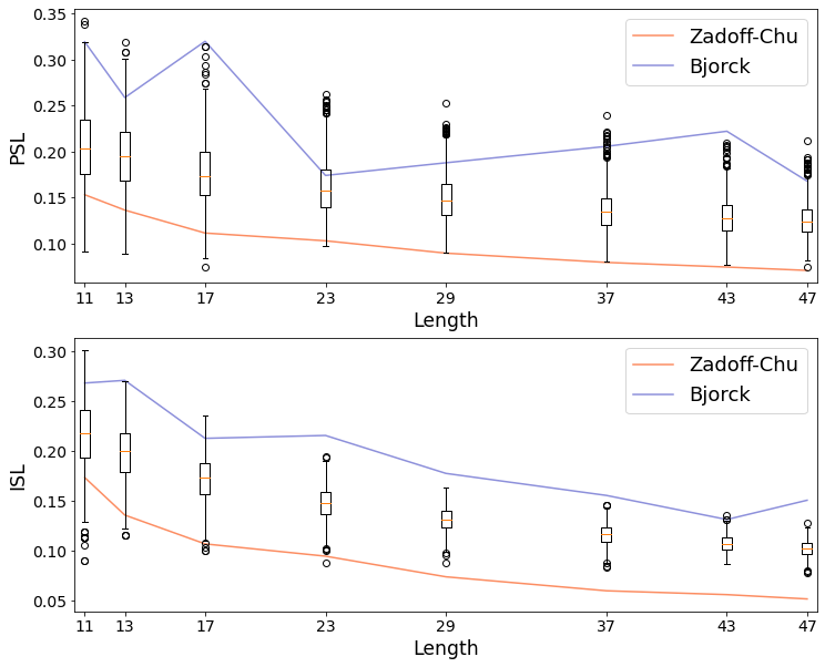
Figure 3: Top: The PSLs of each numerically found CAZAC are compared to the Zadoff-Chu and Björck sequences by box plot. Bottom: The ISLs of each numerically found CAZAC are compared to the Zadoff-Chu and Björck sequences by box plot. Notably, it seems possible to get better PSL and ISL than the Zadoff-Chu sequence in some cases.

To further illustrate the properties of CAZAC sequences generated by these methods, we juxtapose the (modulus) of the ambiguity function of a length 43 numerically found CAZAC sequence and the typically used used Zadoff-Chu sequence. This is depicted in Fig. 4.

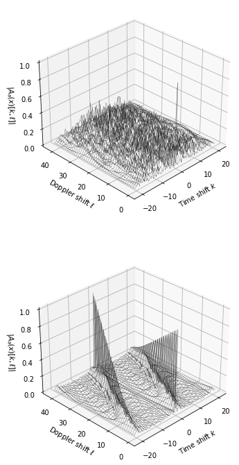
Figure 4: Top: Ambiguity function plot for a computed length 43 CAZAC sequence. Bottom: Ambiguity function plot for the length 43 Zadoff-Chu sequence. Although not as flat as the Zadoff-Chu sequence, the energy is more well spread in the computed sequence so no values exceed 0.3 times the ambiguity function at $(k,\ell)=(0,0)$.

VII Future Directions

This work provides a framework for computing CAZAC sequences by using nonlinear sum of squares optimization. In addition to the potential problem of spurious local minima, scalability is an issue as well. It is possible that other optimization methods or equation solvers would lead to improved efficiency. The code has been made available through GitHub to help ensure replicability of the numerical experiments and to provide a base of code for future directions of work.

It is also likely that the system of equations defining CAZAC sequences has some symmetries or redundancies. Exploring these could make it possible to reduce the number of equations and find new sequences more efficiently.

Another alternative is to convert the aperiodic autocorrelations into a system of polynomials of real variables. We could then use the resulting function to create objective functions that act as a proxy for PSL or ISL and run an optimization search. This could also give us insight on what the optimal PSL and ISL values are for phase-coded waveforms.

Since this work involves an algebraic variety, it is useful to consider techniques from numerical algebraic geometry. For example, homotopy continuation [1] is a framework for analyzing isolated solutions of algebraic varieties. This could be useful in determining whether there are finitely many CAZAC sequences in currently unknown cases.

References

- [1] JC Alexander and James A Yorke. The homotopy continuation method: numerically implementable topological procedures. Transactions of the American Mathematical Society, 242:271–284, 1978.
- [2] John J Benedetto, Katherine Cordwell, and Mark Magsino. Cazac sequences and haagerup’s characterization of cyclic n-roots. In New Trends in Applied Harmonic Analysis, Volume 2, pages 1–43. Springer, 2019.
- [3] John J Benedetto and Jeffrey J Donatelli. Ambiguity function and frame-theoretic properties of periodic zero-autocorrelation waveforms. IEEE Journal of Selected Topics in Signal Processing, 1(1):6–20, 2007.
- [4] Göran Björck. Functions of modulus 1 on Zn whose fourier transforms have constant modulus, and “cyclic n-roots”. In Recent Advances in Fourier Analysis and its Applications, pages 131–140. Springer, 1990.
- [5] Göran Björck and Ralf Fröberg. A faster way to count the solutions of inhomogeneous systems of algebraic equations, with applications to cyclic n-roots. Journal of Symbolic Computation, 12(3):329–336, 1991.
- [6] Göran Björck and Bahman Saffari. New classes of finite unimodular sequences with unimodular fourier transforms. circulant hadamard matrices with complex entries. Comptes rendus de l’Académie des sciences. Série 1, Mathématique, 320(3):319–324, 1995.
- [7] Zhenhua Feng, Ming Tang, Songnian Fu, Lei Deng, Qiong Wu, Rui Lin, Ruoxu Wang, Ping Shum, and Deming Liu. Performance-enhanced direct detection optical OFDM transmission with CAZAC equalization. IEEE Photonics Technology Letters, 27(14):1507–1510, 2015.
- [8] Uffe Haagerup. Cyclic p-roots of prime lengths p and related complex hadamard matrices. arXiv preprint arXiv:0803.2629, 2008.
- [9] Mohammad M Mansour. Optimized architecture for computing zadoff-chu sequences with application to lte. In GLOBECOM 2009-2009 IEEE Global Telecommunications Conference, pages 1–6. IEEE, 2009.
- [10] Andrzej Milewski. Periodic sequences with optimal properties for channel estimation and fast start-up equalization. IBM Journal of Research and Development, 27(5):426–431, 1983.
- [11] Wai Ho Mow. A unified construction of perfect polyphase sequences. In Proceedings of 1995 IEEE International Symposium on Information Theory, page 459. IEEE, 1995.
- [12] Wai Ho Mow and S-YR Li. Aperiodic autocorrelation properties of perfect polyphase sequences. In [Proceedings] Singapore ICCS/ISITA92, pages 1232–1234. IEEE, 1992.
- [13] Ki-Hyeon Park, Hong-Yeop Song, Dae San Kim, and Solomon W Golomb. Optimal families of perfect polyphase sequences from the array structure of fermat-quotient sequences. IEEE Transactions on Information Theory, 62(2):1076–1086, 2015.
- [14] DE Vakman. The ambiguity function in the statistical theory of radar. In Sophisticated Signals and the Uncertainty Principle in Radar, pages 98–125. Springer, 1968.
- [15] Krzysztof Wesolowski, Adrian Langowski, and Krzysztof Bakowski. A novel pilot scheme for 5g downlink transmission. In 2015 International Symposium on Wireless Communication Systems (ISWCS), pages 161–165. IEEE, 2015.