Theory-independent randomness generation with spacetime symmetries

Abstract

We introduce a class of semi-device-independent protocols based on the breaking of spacetime symmetries. In particular, we characterise how the response of physical systems to spatial rotations constrains the probabilities of events that may be observed: in our setup, the set of quantum correlations arises from rotational symmetry without assuming quantum physics. On a practical level, our results allow for the generation of secure random numbers without trusting the devices or assuming quantum theory. On a fundamental level, we open a theory-agnostic framework for probing the interplay between probabilities of events (as prevalent in quantum mechanics) and the properties of spacetime (as prevalent in relativity).

Introduction. Quantum field theory and general relativity, as they currently stand, describe two distinct classes of physical phenomena: probabilities of events on the one hand, and spacetime geometry on the other. Large efforts are currently underway to construct a theory of quantum gravity that would describe both classes of phenomena and their interaction in a unified way. Given the difficulties in this endeavour, one may start with a more modest, but nonetheless illuminating approach: analyse how probabilities of detector clicks and properties of spacetime interact, and what constraints they impose on one another. Here, we propose to use semi-device-independent (semi-DI) quantum information protocols to study this interrelation.

DI and semi-DI approaches mayers1998quantum ; barrett2005no ; colbeck ; acin2007device ; gallego2010device ; pawlowski2011semi ; liang2011semi ; branciard2012one ; VanHimbeeck2017 treat devices in an experiment as “black boxes”: no assumptions (or only very mild ones) are made about the inner workings of the devices, and the analysis relies on the observed input-output statistics alone. While Bell and other DI black-box scenarios have previously been used to study the foundations of quantum theory brunner2014bell ; scarani2019bell , here we suggest to “put the boxes into space and time”.

Specifically, we consider the prepare-and-measure scenario sketched in Fig. 1, which can be used to generate random numbers that are secure against eavesdroppers with additional classical information li2011semi ; acin2016certified ; ma2016quantum ; VanHimbeeck2017 ; rusca2019self ; tebyanian2021semi . We define a class of semi-DI quantum random number generators based on an assumption about how the transmitted system may respond to spatial rotations. Crucially, this semi-DI assumption is representation-theoretic in nature, thus recapturing the theory-independence characteristic of the DI regime. We show that the exact shape of the set of quantum correlations in this setup appears to emerge as a direct consequence of the symmetries of spacetime, which also entails the security of our protocol against post-quantum eavesdroppers.

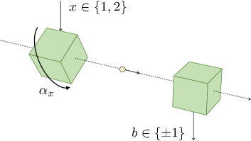
Figure 1: Setup: A fixed but arbitrary state is generated in the preparation device $P$, which is rotated by an angle $\alpha_{x}\in\{0,\alpha\}$ relative to the measurement device $M$ according to an input setting $x\in\{1,2\}$. The state is then sent to $M$, where a measurement yields one of two outcomes $b\in\{\pm 1\}$.

The setup. We consider a semi-DI random number generator similar to the one described in VanHimbeeck2017 ; van2019correlations , given by the prepare-and-measure scenario depicted in Fig. 1. The goal is to generate statistics $P(b|x)$ that certify that even external eavesdroppers with additional (classical) knowledge cannot predict $b$. As in standard DI quantum information, the security of semi-DI protocols does not require any assumptions on the inner-workings of the devices, but it requires some constraint on the physical system that is communicated between the devices gallego2010device ; bowles2014certifying ; VanHimbeeck2017 . This has often been implemented with a bound on the dimension of the Hilbert space of the transmitted system, restricting the communication to qubits or qutrits, as in gallego2010device ; li2011semi ; bowles2014certifying ; brunner2008testing , although this is arguably not very well-motivated for non-idealised physical scenarios. An alternative scheme was provided in VanHimbeeck2017 ; van2019correlations , in which the mean value of some observable $H$ (such as the energy of the transmitted system) was constrained. This formulation, however, requires one to assume the validity of quantum theory, which is a restriction we would like to avoid for our purpose. In fact, the physical meaning of $H$ (say, as the generator of time translations) plays no direct role in their analysis. Here, instead, we propose semi-DI assumptions on quantities like spin or energy, which anchor the security of the resulting protocols on properties of spacetime physics that are directly related to the interpretation of these quantities.

Quantum boxes. Let us start by describing the setup in terms of quantum theory, which we will later generalise to a theory-agnostic description. We consider two devices (Fig. 1). The first device prepares some quantum state $\rho_{1}$ and takes an input $x\in\{1,2\}$. The experimenter either does nothing to the device (i.e. applies $R_{0}=\mathds{1}$ if $x=1$), or rotates it by an angle $\alpha$ around a fixed axis relative to the other device (i.e. applies the rotation $R_{\alpha}$, if $x=2$). After the rotation, the physical system is prepared and sent to the second device. The second device produces an outcome $b\in\{\pm 1\}$, and is described by a POVM $\{M_{b}\}$. Minimal assumptions are made about the devices pironio2016focus , such that $\rho_{1}$ and $M_{b}$ are treated as unknown and may fluctuate according to some shared random variable $\lambda$.

While we allow such shared randomness (see Eq. (7) below), we do not allow shared entanglement between preparation and measurement devices, which is a standard assumption in the semi-DI context Pauwels . Disallowing this, and demanding that the full preparation device is rotated, prevents the rotation from being applied only to a part of the emitted system, which in turn prevents the appearance of detectable relative phases like $(-1)$ for a $2\pi$-rotation of spin-$1/2$ fermions.

Well-known arguments (e.g. in (Wald, , Sec. 13.1)) imply that fundamental symmetries, such as the rotations $R_{\alpha}$, must act as unitary transformations $U_{\alpha}$ on Hilbert space, furnishing a projective representation of the symmetry group (here ${\rm SO}(2)$). The finite-dimensional projective unitary representations of SO(2) arise from unitary representations of the translation group ($\mathbb{R},+)$ and are of the form ${U}_{\alpha}=e^{i\phi\alpha}\bigoplus_{k}e^{ik\alpha}$, where $k$ runs over a subset of $\mathbb{Z}$ and can appear with some multiplicity, and $\phi\in\mathbb{R}$. To implement an assumption about the response of the system to rotations, we upper bound the absolute value of the labels $j=k+\phi$ in ${U}_{\alpha}$. Then, we can restrict to representations of the form

$${U}_{\alpha}=\bigoplus_{j=-J}^{J}n_{j}e^{ij\alpha},$$ (1)

where $j$ runs over either integers or half-integers, and $n_{j}$ indicates how many copies of the $j$-th irrep of the translation group are contained in ${U}_{\alpha}$. For details see Supplemental Material I, where we also show that it is sufficient to consider representations on Hilbert spaces; in principle, we could consider systems containing incoherent mixtures of both fermions and bosons, but such cases can be reduced to correlations deriving from the Hilbert space attached to the system of the highest $J$.

Fixing some $J\in\{0,\frac{1}{2},1,\frac{3}{2},\ldots\}$ introduces an assumption on the physical system that is sent from the preparation to the measurement device, namely, on its possible response to spatial rotations. This is what makes our scenario semi-DI, and what replaces the more common assumption on the Hilbert space dimension of the transmitted system. It is important to note that we do not fix the numbers $n_{j}$, thus allowing for the number of copies to vary, i.e. the Hilbert space dimension is not bounded by this. Furthermore, the decomposition of ${U}_{\alpha}$ into its irreducible representations (irreps) leads to a decomposition of the Hilbert space into $\mathcal{H}=\bigoplus_{j=-J}^{J}\mathcal{H}_{j}$, where ${\mathrm{dim}}(\mathcal{H}_{j})=n_{j}$. If we have a particle with internal degrees of freedom given by $\mathcal{H}$, then $J$ bounds the spin of the particle. This setup could e.g. be realized by a single photon being sent through a polarizer, with a relative rotation between the two devices, and “spin” (helicity) $J=1$ (or $J=N$ for $N$ photons caban2003photon ).

We are interested in the possible correlations between outcome $b$ and setting $x$ that can be obtained under an assumption on $J$ via Eq. (1) in the quantum case. Let us for the moment assume that the initial state $\rho_{1}$ is a pure state $\rho_{1}=\outerproduct{\phi_{1}}{\phi_{1}}$, then

$$\mathcal{Q}_{J,\alpha}\coloneqq\{(E_{1},E_{2})|E_{x}=\langle\phi_{x}|M|\phi_{x}\rangle,\ket{\phi_{2}}=U_{\alpha}\ket{\phi_{1}}\},$$ (2)

where $M=M_{1}-M_{-1}$ is an observable constructed from the POVM $\{M_{b}\}$ such that $E_{x}=P(+1|x)-P(-1|x)$ characterises the bias of the outcome toward $\pm 1$ for a given $x$. In VanHimbeeck2017 it was shown that when the states that may be sent have overlap $\gamma\geq|\langle\phi_{1}|\phi_{2}\rangle|$, the set of possible correlations is characterised by the inequality

$$\frac{1}{2}\left(\sqrt{1+E_{1}}\sqrt{1+E_{2}}+\sqrt{1-E_{1}}\sqrt{1-E_{2}}\right)\geq\gamma.$$ (3)

We show in Supplemental Material II that for our scenario,

$$\gamma=\min|\langle\phi_{1}|\phi_{2}\rangle|=\left\{\begin{matrix}\cos(J\alpha)&\mbox{if}&|J\alpha|<\frac{\pi}{2}\\ 0&\mbox{if}&|J\alpha|\geq\frac{\pi}{2}\end{matrix}\right..$$ (4)

The bound $\gamma$ describes the smallest possible overlap of any initial state with its rotation by $\alpha$, given that the absolute value of its spin is at most $J$. From VanHimbeeck2017 , it follows that (3) and (4) define some set of correlations $\widetilde{\mathcal{Q}}_{J,\alpha}$ (see Fig. 2), of which we know that our set of interest is a subset: ${\mathcal{Q}}_{J,\alpha}\subseteq\widetilde{\mathcal{Q}}_{J,\alpha}$. In Supplemental Material III, we show that the two sets are in fact identical: the extremal boundary of $\widetilde{\mathcal{Q}}_{J,\alpha}$ can be realised via rotations of the family of states $(|j\rangle+e^{i\theta}|-j\rangle)/\sqrt{2}$, hence $\mathcal{Q}_{J,\alpha}=\widetilde{\mathcal{Q}}_{J,\alpha}$.

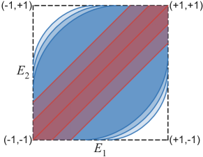
Figure 2: The quantum and classical sets $\mathcal{Q}_{J,\alpha}$ (dark blue) and $\mathcal{C}_{J,\alpha}$ (dark red; line $|E_{2}-E_{1}|=0$), and the quantum and classical relaxed sets $\mathcal{Q}^{\delta}_{J,\alpha}$ and $\mathcal{C}^{\delta}_{J,\alpha}$ for $\delta\in\{0.15,0.3\}$. We set $J=1$ and $\alpha=0.66$ throughout.

The set $\mathcal{Q}_{J,\alpha}$ grows with $J\alpha$ until $J\alpha=\pi/2$, at which point a $\ket{\phi_{1}}$ exists such that $|\phi_{2}\rangle=U_{\alpha}\ket{\phi_{1}}$ is orthogonal to it. If $|\phi_{1}\rangle$ and $|\phi_{2}\rangle$ are perfectly distinguishable, there exist (even deterministic) strategies to generate all conceivable correlations.

Anticipating the generation of private randomness as discussed further below, we define classical correlations as convex combinations of deterministic behaviours, i.e. $\mathbf{E}^{\lambda}:=(E_{1},E_{2})\in\{\pm 1\}\times\{\pm 1\}$, that again satisfy the maximum spin $J$ bound:

$$\mathcal{C}_{J,\alpha}\coloneqq\{\mathbf{E}=\sum_{\lambda}p(\lambda)\mathbf{E}^{\lambda}\,\,|\,\,\mathbf{E}^{\lambda}\in\mathcal{Q}_{J,\alpha},\mathbf{E}^{\lambda}\in\{\pm 1\}\times\{\pm 1\}\},$$ (5)

where $\{p(\lambda)\}_{\lambda}$ is a probability distribution. If $J\alpha<\pi/2$, the states are not perfectly distinguishable, and so correlations are limited to $\mathbf{E}^{\lambda}=(\pm 1,\pm 1)$; alternatively, if $J\alpha\geq\pi/2$, the states can be perfectly distinguishable, and so $\mathbf{E}^{\lambda}=(\pm 1,\mp 1)$ are also possible correlations. Convex combinations of the former case gives the set $\mathcal{C}_{J,\alpha}=\{(E_{1},E_{2})|-1\leq E_{1}=E_{2}\leq 1\}$, whilst the latter case gives all possible correlations.

So far only pure states have been considered. However, it turns out that this is sufficient, as the set of mixed state correlations, defined by

$$\ \mathcal{Q}^{\prime}_{J,\alpha}\coloneqq\{(E_{1},E_{2})\,\,|\,\,E_{x}={\mathrm{tr}}(M\rho_{x}),\rho_{2}=U_{\alpha}\rho_{1}U^{\dagger}_{\alpha}\},$$ (6)

coincides precisely with $\mathcal{Q}_{J,\alpha}$. Clearly $\mathcal{Q}_{J,\alpha}\subseteq\mathcal{Q}_{J,\alpha}^{\prime}$, and the converse $\mathcal{Q}_{J,\alpha}^{\prime}\subseteq\mathcal{Q}_{J,\alpha}$ can be proven by purifying arbitrary states $\rho$ using an ancilla system, without adding any spin (for details, see Supplemental Material IV). Thus, the set $\mathcal{Q}_{J,\alpha}$ is convex, which means that it also describes scenarios where preparation $\rho_{1}$ and measurements $M_{b}$ fluctuate according to some shared random variable $\lambda$ distributed $\sim p(\lambda)$, i.e.

$$P(b|\alpha)=\sum_{\lambda}p(\lambda){\rm tr}(M_{b}(\lambda)U_{\alpha}\rho_{1}(\lambda)U_{\alpha}^{\dagger})$$ (7)

(where the input $x\in\{0,\alpha\}$ is chosen independently from $\lambda$). So far we have assumed that the constraint on the maximum spin $J$ holds exactly and in every run of the experiment. However, in a more realistic scenario, one may want to grant room for imperfections. This can be taken into account by trusting only that the constraint strictly holds with probability $1-\delta$, with $0\leq\delta<1$, but for probability $\delta$ the system might carry arbitrarily high spin. This leads to the relaxed quantum set

$$\mathcal{Q}^{\delta}_{J,\alpha}=(1-\delta)\mathcal{Q}_{J,\alpha}+\delta\,\left([-1,+1]\times[-1,+1]\right)$$ (8)

depicted in Fig. 2, where ${\mathrm{conv}}$ denotes the convex hull Webster . Similarly, replacing $\mathcal{Q}$ by $\mathcal{C}$ in this expression defines the classical relaxed set $\mathcal{C}_{J,\alpha}^{\delta}$. For a full characterisation of the relaxed quantum and classical sets, see Supplemental Material V, where we also discuss types of experimental uncertainties for which these sets are physically relevant. For example, we show that for coherent states, where the photon number $n$ follows a Poisson distribution on Fock space, the relaxed quantum set $\mathcal{Q}^{\delta}_{J,\alpha}$ with $\delta=\mathcal{O}(\eta^{1/4})$ contains the relevant set of possible correlations, with $\eta:={\rm Prob}(n>N)$ giving the probability of a constraint on $J(=N)$ failing (which tends to zero exponentially in $N$).

Generating private randomness. Adapting the results of van2019correlations , we can show that correlations in $\mathcal{Q}_{J,\alpha}$ outside of the classical set admit the generation of private randomness. Consider an eavesdropper Eve with classical (but no quantum) side information who tries to guess the value of $b$. Alice, who uses the setup of Fig. 1 to generate private random outcomes $b$, will in general not have complete knowledge of all variables $\lambda\in\Lambda$ of relevance for the experiment, which is expressed in Eq. (7) by $P(b|x)$ being the mixture $\sum_{\lambda}p(\lambda)P(b|x,\lambda)$. Eve, however, may have additional relevant information $\lambda$ (in addition to knowing the inputs $x$), and Alice would thus like to guarantee that the conditional entropy $H(B|X,\Lambda)=-\sum_{b,x,\lambda}p(b,x,\lambda)\log_{2}p(b|x,\lambda)$ is large, quantifying Eve’s difficulty to predict $b$. Since $H(B|X,\Lambda)=\sum_{\lambda}p(\lambda)H(\mathbf{E}^{\lambda})$ where $H(\mathbf{E}):=-\frac{1}{2}\sum_{b,x}\frac{1+bE_{x}}{2}\log\frac{1+bE_{x}}{2}$ , the amount of conditional entropy $H^{\star}$ that Alice can guarantee if she observes correlations $\mathbf{E}=(E_{1},E_{2})$, i.e. $H(B|X,\Lambda)\geq H^{\star}$, is determined by the optimisation problem

$$H^{\star} = \min_{\{p(\lambda),\mathbf{E}^{\lambda}\}}\sum_{\lambda}p(\lambda)H(\mathbf{E}^{\lambda})$$ (9)

$$\mbox{subject to }\sum_{\lambda:\mathbf{E}^{\lambda}\in\mathcal{Q}^{\omega}_{J,\alpha}}p(\lambda)\geq 1-\varepsilon$$

$$\mbox{and }\sum_{\lambda}p(\lambda)\mathbf{E}^{\lambda}=\mathbf{E}.$$

That is, $H^{\star}$ tells us the number of certified bits of private randomness against Eve, under the assumption that the transmitted systems have spin at most $J$ — or, rather, when this assumption holds approximately (up to some $\omega$), with high probability $(1-\varepsilon)$. This quantity is non-zero, $H^{\star}\equiv H^{\star}_{\varepsilon,\omega,\alpha}>0$, whenever the observed correlations are outside of the relaxed classical set, $\mathbf{E}\not\in\mathcal{C}^{\varepsilon}_{J,\alpha}$. For $\varepsilon=\omega=0$, this optimisation problem is equivalent to the one in (van2019correlations, , Sec. 3.2) for the case that there is, in the terminology of that paper, no max-average assumption (see Supplemental Material  VI). For determining the numerical value of $H^{\star}_{0,0,\alpha}$, we thus refer the reader to van2019correlations . Furthermore, as we show in Supplemental Material VII, we have a robustness bound for $H^{\star}_{\varepsilon,\omega,\alpha}$, which reads

$$H_{0,0,\alpha}^{\star}\geq H_{\varepsilon,\omega,\alpha}^{\star}\geq H^{\star}_{0,0,\alpha+c(\varepsilon+\omega)}+\log(1-\varepsilon)-\frac{\varepsilon\log(2/\varepsilon)}{1-\varepsilon},$$

where $c=2\cot(J\alpha)/J$. Thus, for small $\varepsilon,\omega>0$, the number of certified random bits can still be well approximated by using the results of van2019correlations for $\varepsilon=\omega=0$.

Rotation boxes. We now drop the assumption that quantum theory holds, and consider the most general form the probabilities $P(b|\alpha)$ may take that is consistent with the rotational symmetry of the setup while implementing our spin bound. Due to the $(2\pi)$-periodicity of the setup, we can develop $P(b|\alpha)$ into a Fourier series, given sufficient regularity in $\alpha$. We argue that the semi-DI bound on the maximal spin $J$ translates into the condition that this series has to terminate at $2J$, i.e. that

$$P(b|\alpha)=\sum_{k=0}^{2J}\left(c_{k}^{(b)}\cos(k\alpha)+s_{k}^{(b)}\sin(k\alpha)\right),$$ (10)

with suitable coefficients $c_{k}^{(b)}$, $s_{k}^{(b)}$. In fact, if $P(b|\alpha)$ satisfies Eq. (7) and $U_{\alpha}$ satisfies the semi-DI assumption Eq. (1), then it is of the form (10). This can be seen by expanding the complex exponentials appearing in $U_{\alpha}$ and collecting sine and cosine terms (see Supplemental Material VIII). However, such “rotation boxes” (10) are more general: no assumptions are made on the existence of quantum states, measurements, or representations of ${\rm SO}(2)$ on Hilbert spaces that would reproduce $P(b|\alpha)$. We can think of these $P(b|\alpha)$ as “black boxes” that accept a spatial rotation by angle $\alpha$ as input, and produce an output $b$, in any possible world where it makes sense to talk about outcome probabilities and spacetime symmetries, even if quantum theory does not necessarily hold.

Similar arguments as in the quantum case Wald imply that there must be a representation of ${\rm SO(2)}$ on the space of ensembles of boxes (in QT, on the density matrices), and $2J$ is the maximal label appearing in this representation. This “post-quantum number” $J$ behaves in ways that resemble its quantum counterpart. For example, placing two independent rotation boxes $P_{1}$ and $P_{2}$ side by side gives a resulting box $P(b_{1},b_{2}|\alpha):=P_{1}(b_{1}|\alpha)P_{2}(b_{2}|\alpha)$ with $J=J_{1}+J_{2}$. This is in line with particle physics intuition by hinting at $J$ being related to the number of constituents or “size” of the physical system.

Since $P(+1|\alpha)+P(-1|\alpha)=1$, the set of possible spin-$J$ quantum and rotation boxes respectively can be denoted by

$$\mathcal{Q}_{J} := \{\alpha\mapsto P(+1|\alpha)\,\,|\,\,P(b|\alpha)\mbox{ is of the form }(\ref{eqQuantum})\},$$

$$\mathcal{R}_{J} := \{\alpha\mapsto P(+1|\alpha)\,\,|\,\,P(b|\alpha)\mbox{ is of the form }(\ref{SBs})\},$$

where, for $\mathcal{Q}_{J}$, we assume that $U_{\alpha}$ is of the form (1). We have just seen that $\mathcal{Q}_{J}\subseteq\mathcal{R}_{J}$. Trivially, $\mathcal{Q}_{0}=\mathcal{R}_{0}$ is the set of constant probability functions, and it can be shown that $\mathcal{Q}_{1/2}=\mathcal{R}_{1/2}$ (see Supplemental Material IX). However, in upcoming work InPreparation , we show that $\mathcal{Q}_{J}\subsetneq\mathcal{R}_{J}$, i.e. that there are more general ways to respond to spatial rotations than allowed by quantum theory, if $J\geq 3/2$.

Agreement of correlation sets. If we consider only two possible inputs, $x\in\{1,2\}$, with corresponding rotations by $0$ and $\alpha$ (which is a fixed angle), the resulting set of rotation box correlations is

$$\mathcal{R}_{J,\alpha} \coloneqq \{(E_{1},E_{2})|E_{1}=P(+1|0)-P(-1|0),$$ (11)

$$E_{2}=P(+1|\alpha)-P(-1|\alpha),P\,\mbox{as in}\,(\ref{SBs})\}$$

Obviously $\mathcal{Q}_{J,\alpha}\subseteq\mathcal{R}_{J,\alpha}$, but we can say more:

Theorem 1.

For every fixed angle $\alpha$, the quantum set coincides with the rotation box set, i.e. $\mathcal{Q}_{J,\alpha}=\mathcal{R}_{J,\alpha}$.

Proof.

We use (DeVore, , Chapter 4, Thm. 1.1): If $T$ is a trigonometric polynomial of degree $n$ with $-1\leq T(x)\leq 1\;\forall x$, then

$$T^{\prime}(x)^{2}+n^{2}T(x)^{2}\leq n^{2}.$$ (12)

Define $T(\alpha)\coloneqq P(+|\alpha)-P(-|\alpha)=1-2P(+|\alpha)$, which is a trigonometric polynomial of degree $n=2J$ with $-1\leq T(\alpha)\leq 1$. Rewrite (12) as $T^{\prime}(x)\leq 2J\sqrt{1-T(x)^{2}}$ and set $E_{x}:=T(0)$ and $E_{x^{\prime}}:=T(\alpha_{\varepsilon})$, then

$$\alpha_{\varepsilon}=\int_{0}^{\alpha_{\varepsilon}}d\alpha \geq\int_{0}^{\alpha_{\varepsilon}}\frac{T^{\prime}(\alpha)d\alpha}{2J\sqrt{1-T(\alpha)^{2}}}=\frac{1}{2J}\int_{E_{x}}^{E_{x^{\prime}}}\frac{dy}{\sqrt{1-y^{2}}}$$

$$=\frac{1}{2J}\left(\arcsin E_{x^{\prime}}-\arcsin E_{x}\right),$$

where we have substituted $y=T(\alpha)$. It follows that

$$\frac{1}{2}|\arcsin E_{2}-\arcsin E_{1}|\leq J\alpha.$$ (13)

For $J\alpha\geq\pi/2$, the set $\mathcal{R}_{J,\alpha}$ contains all possible correlations, as in the quantum case. For $J\alpha<\pi/2$, taking the cosine of both sides of (13) reproduces, after some elementary manipulations (see Supplemental Material X), precisely the conditions of the quantum set, as in (3) and (4), hence $\mathcal{R}_{J,\alpha}\subseteq\mathcal{Q}_{J,\alpha}$. ∎

This shows that the set of quantum correlations in our setup can be understood completely and exactly as a consequence of the interplay of probabilities and spatial symmetries. Notably, tavakoli2022informationally also identify a general polytope $\mathcal{G}$ that characterises the set of correlations under an abstract informational restriction tavakoli2020informationally when no assumption is made on the underlying physical theory, and in the simplest case of two inputs, this polytope agrees with the set of achievable quantum correlations. Here, however, we show that a physically well-motivated assumption reproduces the curved boundary of the set of quantum correlations exactly, for all $J$.

Post-quantum security. The equality $\mathcal{R}_{J,\alpha}=\mathcal{Q}_{J,\alpha}$ implies that the semi-DI protocol above is secure against post-quantum eavesdroppers. While Alice observes quantum correlations $\bm{E}\in\mathcal{Q}_{J,\alpha}$, i.e. of the form (7), it is conceivable that these are actually mixtures of beyond-quantum rotation boxes $\bm{E}^{\lambda}\in\mathcal{R}_{J,\alpha}^{\omega}$ such that $\bm{E}=\sum_{\lambda}p(\lambda)\bm{E}^{\lambda}$, where Eve may have access to beyond-quantum physics and know the value of $\lambda$. To see how many bits of private randomness $H^{\star}$ Alice can guarantee against Eve in this case, the optimisation problem (9) has to be altered by relaxing the condition on $\mathbf{E}^{\lambda}\in\mathcal{Q}_{J,\alpha}^{\omega}$ to $\mathbf{E}^{\lambda}\in\mathcal{R}_{J,\alpha}^{\omega}$, i.e. by only demanding that every transmitted system is, up to probability $\varepsilon$, approximately a (not necessarily quantum) rotation box of maximal spin $J$. However, since $\mathcal{R}_{J,\alpha}^{\omega}=\mathcal{Q}_{J,\alpha}^{\omega}$, the optimisation problem and hence $H^{\star}$ are unaffected by this.

Conclusions. We have introduced a theory-independent and semi-device-independent scenario for generating random numbers based on the response of physical systems to spatial rotations. This allowed us to recover the exact set of quantum correlations of the setup without assuming quantum mechanics, merely from a semi-DI assumption on a generalized notion of spin of the transmitted system. From a fundamental point of view, our results demonstrate that the symmetries of space and time enforce important features of quantum theory in some scenarios. From a more pragmatic point of view, they allow us to certify random numbers from physically better motivated assumptions than the usual dimension bounds, and guarantee security even against eavesdroppers with additional classical knowledge and access to post-quantum physics.

While we have focused on spatial ${\rm SO}(2)$ rotations for simplicity, the elements of our framework can obviously be generalized to other symmetry groups such as the group of rotations ${\rm SO(3)}$, the group of time translations $\mathbb{R}$, or the Lorentz group, and to other causal scenarios. We will analyze this more general setting in future work InPreparation , building on the earlier results of Garner2020 .

In addition to several open technical questions, our work suggests an interesting foundational question: is quantum theory perhaps the only probabilistic theory that “fits into space and time” for all scenarios? A positive answer to this question would significantly improve our understanding of the logical architecture of our world. On the other hand, a negative answer could inform experimental tests of quantum theory, by telling us where there might be elbow room for beyond-quantum physics consistent with spacetime as we know it.

Acknowledgments. We are grateful to Valerio Scarani and Armin Tavakoli for helpful discussions. We acknowledge support from the Austrian Science Fund (FWF) via project P 33730-N. This research was supported in part by Perimeter Institute for Theoretical Physics. Research at Perimeter Institute is supported by the Government of Canada through the Department of Innovation, Science, and Economic Development, and by the Province of Ontario through the Ministry of Colleges and Universities.

Supplemental Material

I Projective Representations of SO(2)

In this section, we want to analyse the representations of SO(2). We will restrict our discussion to representations on finite-dimensional Hilbert spaces. In general, we consider projective unitary representation of SO(2). In finite dimension it is always possible to deprojectivise unitary representations of the connected Lie group $\mathcal{G}$ by passing them to unitary representations of its universal cover $\hat{\mathcal{G}}$, and moreover, every projective unitary representation of $\mathcal{G}$ stems from a ordinary unitary representation of $\hat{\mathcal{G}}$ hall2013 . It can be checked that the universal cover of SO(2) is the translation group $(\mathbb{R},+)$ hatcher2002 ; hall2015 . Using Stone’s theorem stone1932 , we find that the projective representations of SO(2) must be (up to a global phase) of the form

$$U_{\alpha}=\exp(i\,\mbox{diag}(\begin{matrix}j_{1},&\ldots,&j_{N}\end{matrix})\alpha),$$

where all $j_{i}\in\mathbb{R}$, $\alpha\in\mathbb{R}$, and $U_{2\pi n}=e^{i\phi_{n}}\mathds{1}$ with $\phi_{n}\in\mathbb{R}$.

From $U_{2\pi}=\exp(i\phi 2\pi)\mathds{1}$, it follows that

$$j_{i}=\phi+k$$ (14)

where $k\in\mathbb{Z}$. It is easy to check that every $U_{\alpha}$ of the form

$$U_{\alpha}=e^{i\phi\alpha}\bigoplus_{k\in\mathbb{Z}}n_{k}e^{ik\alpha},$$

where $\phi\in\mathbb{R}$, $n_{k}\in\mathbb{N}_{0}$, and only a finite number of the $n_{k}\neq 0$, gives a valid projective representation of SO(2).

At first glance, it seems like that $\phi$ introduces only an (on $\alpha$ depending) global phase, which cannot be observed and thus one might conclude that w.l.o.g we can set $\phi=0$. However, it turns out that $\phi$ plays an important role as soon as we implement our constraint $|j_{i}|\leq J$. An immediate consequence of (14) is that $j_{i}-j_{k}\in\mathbb{Z}$ for all $i,k$. Hence, $|j_{i}|\leq J$ will constrain the number of allowed $j_{k}$ (up to multiplicity $n_{k}$). Namely, the maximal number of different $j_{k}$’s is given by $2\tilde{J}+1$, where $\tilde{J}\in\mathbb{N}_{0}\cup\mathbb{N}/2$ and $\tilde{J}\leq J<\tilde{J}+1$. This implies that we can restrict to projective representations of the form

$$U_{\alpha}=\bigoplus_{j=-J}^{J}n_{j}e^{ij\alpha},$$ (15)

where $J\in\mathbb{N}_{0}\cup\mathbb{N}/2$ and all $j\in\mathbb{N}_{0}$ (i.e. $\phi=0$) or all $j\in\mathbb{N}/2$ (i.e. $\phi=-1/2$) depending on if $J$ is in $\mathbb{N}_{0}$ or $\mathbb{N}/2$.

For a better understanding why we only need to consider representations of the form (15), we look at an example where $J=3/4$ and $j_{1}=-1/4$ and $j_{2}=3/4$. Thus we have a representation

$$U_{\alpha}=n_{1}e^{-i\frac{\alpha}{4}}\oplus n_{2}e^{i\frac{3\alpha}{4}}=e^{i\frac{\alpha}{4}}\left(n_{1}e^{-i\frac{\alpha}{2}}\oplus n_{2}e^{i\frac{\alpha}{2}}\right).$$

However, we can define a new projective representation by $\tilde{U}_{\alpha}=e^{-i\frac{\alpha}{4}}U_{\alpha}$, which is now of the form (15) with maximum $\tilde{J}=1/2$ and both representations will lead to the same observable physics.

So far we only considered representations on Hilbert spaces and thus on pure states. Now, we want to argue that this is actually sufficient. In principle, one could think of situations where in every run the measurement device picks a system associated with a different Hilbert space $\mathcal{H}^{i}$ with a different maximum $J^{i}$ and a different phase $\phi^{i}$ appearing in $U^{i}_{\alpha}$. More generally, we can have physical systems that feature incoherent mixtures of bosonic and fermionic degrees of freedom, in accordance with an univalence superselection rule Wightman . Hence, the most general state space to consider is $\mathcal{S}\left(\bigoplus_{i}\mathcal{H}^{i}\right)$. Then, we have a representation $\mathcal{U}_{\alpha}$ acting on $\mathcal{B}\left(\bigoplus_{i}\mathcal{H}^{i}\right)$, which can be written as

$$\mathcal{U}_{\alpha}(\rho)=\bigoplus_{i}(U^{i}_{\alpha})^{\dagger}\bigoplus_{k}\rho^{k}\bigoplus_{l}U^{l}_{\alpha}=\bigoplus_{i}(U^{i}_{\alpha})^{\dagger}\rho^{i}U^{i}_{\alpha},$$

where $U^{i}_{\alpha}$ is a representation of SO(2) on $\mathcal{H}^{i}$ and $\rho^{i}$ is a subnormalised state acting on $\mathcal{H}^{i}$ and we can interpret $p_{i}={\mathrm{Tr}}(\rho^{i})$ as the probability that the box prepares a state $\widetilde{\rho}^{i}=\rho^{i}/{\mathrm{Tr}}(\rho^{i})\in\mathcal{S}(\mathcal{H}^{i})$. For a POVM element $M_{+}$ the probabilities are given by

$$P(+|\alpha) = {\mathrm{Tr}}(\mathcal{U}_{\alpha}(\rho)M_{+})=\sum_{i}{\mathrm{Tr}}((U^{i}_{\alpha})^{\dagger}\rho^{i}U^{i}_{\alpha}M^{i}_{+})$$ (16)

$$= \sum_{i}p_{i}P_{i}(+|\alpha),$$

where $M^{i}_{+}=\Pi^{i}M_{+}\Pi^{i}$, $\Pi^{i}$ is the projection on $\mathcal{H}^{i}$ and $P_{i}(+|\alpha)={\mathrm{Tr}}((U^{i}_{\alpha})^{\dagger}\widetilde{\rho}^{i}U^{i}_{\alpha}M^{i}_{+})\in\mathcal{Q}_{J^{i}}$. Now let $\mathcal{H}^{m}$ be the subspace with the highest maximal spin i.e. $J^{i}\leq J^{m}$, for all $i$. This implies $\mathcal{Q}_{J^{i}}\subseteq\mathcal{Q}_{J^{m}}$ for all $i$, and in particular, we have $P_{i}(+|\alpha)\in\mathcal{Q}_{J^{m}}$. Thus, probabilities $P(+|\alpha)$ of the form (16) are convex combinations of elements of $\mathcal{Q}_{J^{m}}$ and hence $P(+|\alpha)\in\mathcal{Q}_{J^{m}}$. It follows that we could have found the same correlations only by considering the representation $U^{m}_{\alpha}$. This implies that we can restrict to representations of the form (15) without loss of generality.

II Bounding the overlap $\gamma$

To prove the bound (4) on the overlap, it is sufficient to assume $|J\alpha|<\frac{\pi}{2}$ since the other case is trivial. To this end, we evaluate the inner product of an arbitrary state $\ket{\phi}=\sum_{j}\phi_{j}\ket{\psi_{j}}$ and the rotated state $U_{\alpha}\ket{\phi}=\sum_{k}e^{ij\alpha}\phi_{j}\ket{\psi_{j}}$. Using that $|z|\geq{\rm Re}(z)$ for $z\in\mathbb{C}$, we obtain

$$\gamma =\absolutevalue{\bra{\phi}U_{\alpha}\ket{\phi}}$$

$$=\absolutevalue{\sum_{j}|\phi_{j}|^{2}e^{ij\alpha}}$$

$$=\absolutevalue{|\phi_{0}|^{2}+\sum_{j>0}\big{(}|\phi_{-j}|^{2}e^{-ij\alpha}+|\phi_{j}|^{2}e^{ij\alpha}\big{)}}$$

$$\geq|\phi_{0}|^{2}+\sum_{j>0}\cos(j\alpha)\big{(}|\phi_{-j}|^{2}+|\phi_{j}|^{2}\big{)}.$$

There is a factor of $\cos(j\alpha)$ in front of all coefficients, which is smaller for larger $j$, i.e. $\cos(j_{1}\alpha)<\cos(j_{2}\alpha)$ for $j_{1}>j_{2}$ since $|\alpha|\leq\pi/(2J)$. Therefore the final expression is minimised when the coefficients are weighted entirely by the maximum $j$ terms, i.e. for $|\phi_{-J}|^{2}+|\phi_{J}|^{2}=1$, and so $\gamma\geq\cos(J\alpha)$. Moreover, this bound is attained for e.g. $\phi_{J}=\phi_{-J}=1/\sqrt{2}$.

III Identity of the correlation sets, $\mathcal{Q}_{J,\alpha}=\widetilde{\mathcal{Q}}_{J,\alpha}$

In this section, we will assume that $0<J\alpha<\frac{\pi}{2}$, and hence that $0<\cos(J\alpha)<1$. The case $-\frac{\pi}{2}<\alpha<0$ will then follow via symmetry, and all other cases are trivial. From VanHimbeeck2017 , it follows that the set $\mathcal{Q}_{J,\alpha}$ is a subset of the set of general 2-input 2-output quantum correlations $\widetilde{\mathcal{Q}}_{J,\alpha}$ that satisfy

$$\frac{1}{2}\left(\sqrt{1+E_{1}}\sqrt{1+E_{2}}+\sqrt{1-E_{1}}\sqrt{1-E_{2}}\right)\geq\cos(J\alpha).$$ (17)

To show the converse inclusion $\mathcal{Q}_{J,\alpha}\supseteq\widetilde{\mathcal{Q}}_{J,\alpha}$, we will give a convex description of the set of correlations $\widetilde{\mathcal{Q}}_{J,\alpha}$ that are constrained by (17), and then find quantum models for all those correlations, such that the assumptions for $\mathcal{Q}_{J,\alpha}$ are met. First, we rewrite (17) in terms of probabilities. Before we do so, we will fix some notation. As before, we will write $\mathbf{E}=(E_{1},E_{2})$. We will denote pairs of the probabilities that we find for the output “$+$” given settings $0$ and $\alpha$ by $\mathbf{P}^{+}=(P^{+}_{0},P^{+}_{\alpha})=(P(+|0),P(+|\alpha))$. The correlations and the probabilities are related by

$$\mathbf{P}^{+}=\frac{1}{2}\mathbf{E}+\left(\frac{1}{2},\frac{1}{2}\right),$$ (18)

which is a bijective affine transformation, with an affine inverse

$$\mathbf{E}=2\mathbf{P}^{+}-(1,1).$$

Hence, the set $\widetilde{\mathcal{Q}}_{J,\alpha}$ is mapped to a set $\widetilde{\mathcal{Q}}_{J,\alpha}^{P}$ via (18), and $\widetilde{\mathcal{Q}}^{P}_{J,\alpha}$ inherits its convex properties from $\widetilde{\mathcal{Q}}_{J,\alpha}$, and vice versa.

We rewrite (17) as

$$\sqrt{P^{+}_{0}}\sqrt{P^{+}_{\alpha}}+\sqrt{1-P^{+}_{0}}\sqrt{1-P^{+}_{\alpha}}\geq\cos(j\alpha).$$ (19)

It is obvious from Fig. 2, and easy to check formally, that the extremal points of the compact convex set $\widetilde{\mathcal{Q}}_{J,\alpha}^{P}$ are to be found among the corner points $(0,0)$, $(1,1)$, and the two curves for which Eq. (19) holds with equality. These curves $c_{1}$ and $c_{2}$ can be parametrized by a parameter $\tau$, i.e. $c_{i}(\tau)=(P_{0}^{+}(\tau),P_{\alpha}^{+}(\tau))$, such that by a variable $\tau$ via

$$c_{1}(\tau) = (\cos^{2}(J\tau),\cos^{2}(J(\tau+\alpha))\quad(\tau\in I_{1}),$$ (20)

$$c_{2}(\tau) = (\cos^{2}(J\tau),\cos^{2}(J(\tau-\alpha)))\quad(\tau\in I_{2}),$$ (21)

where $I_{1}=\left[0,\frac{\pi}{2J}-\alpha\right]$ and $I_{2}=\left[\alpha,\frac{\pi}{2J}\right]$. To check this for e.g. the curve $c_{1}$, use the addition theorem for the cosine and calculate

$$\sqrt{P_{0}^{+}(\tau)}\sqrt{P_{\alpha}^{+}(\tau)}+\sqrt{1-P_{0}^{+}(\tau)}\sqrt{1-P_{\alpha}^{+}(\tau)}=$$

$$= \cos(J\tau)\cos(J(\tau+\alpha))+\sin(J\tau)\sin(J(\tau+\alpha))$$

$$= \cos(J\alpha);$$

checking equality for the curve $c_{2}$ is analogous. For $\tau=0$, the $c_{1}$ attains $P_{0}^{+}=1$, and for $\tau=\frac{\pi}{2J}-\alpha$, it attains $P_{\alpha}^{+}=0$; hence it describes the complete lower curve that bounds $\widetilde{\mathcal{Q}}_{J,\alpha}^{P}$ in Fig. 2. Similarly, the $c_{2}$ parametrizes the complete upper curve.

Now, we will construct quantum models for all these candidate extreme points using only probability distributions that lead to correlations in $\mathcal{Q}_{J,\alpha}$. The points $(0,0)$ and $(1,1)$ are given by constant probability distributions, and can therefore be trivially constructed. For example, the point $(1,1)$ can be constructed from the state $\ket{J}\in\mathcal{H}_{J}$ and the measurement operators $M_{+}=\outerproduct{J}{J}$ and $M_{-}=\mathds{1}-M_{+}$.

Next, we consider the points $(\cos^{2}(J\tau),\cos^{2}(J(\tau+\alpha)))$ for $\tau\in I_{1}$. We will consider the state $\ket{\phi}=\frac{1}{\sqrt{2}}\left(\ket{-J}+\ket{J}\right)$ and the measurement operators $M_{+}=U_{\tau}^{\dagger}\outerproduct{\phi}{\phi}U_{\tau}$ and $M_{-}=\mathds{1}-M_{+}$, and we can check that this gives us the desired probabilities

$$P^{+}_{0} = P(+|0)=\langle\phi|M_{+}|\phi\rangle=\left|\bra{\phi}U_{\tau}\ket{\phi}\right|^{2}$$

$$= \left|\frac{e^{-iJ\tau}+e^{iJ\tau}}{2}\right|^{2}=\cos^{2}(J\tau),$$

and

$$P^{+}_{\alpha} = P(+|\alpha)=\langle\phi|U_{\alpha}^{\dagger}M_{+}U_{\alpha}|\phi\rangle=\left|\bra{\phi}U_{\tau}U_{\alpha}\ket{\phi}\right|^{2}$$

$$= \left|\bra{\phi}U_{\tau+\alpha}\ket{\phi}\right|^{2}=\cos^{2}(J(\tau+\alpha)).$$

Similarly, for the points $(\cos^{2}(\tau J),\cos^{2}((\alpha-\tau)J))$, where $\tau\in I_{2}$, we can use the same state $\ket{\phi}$ as before, but we have to replace the measurement operators with $M_{+}=U^{\dagger}_{-\tau}\outerproduct{\phi}{\phi}U_{-\tau}$ and $M_{-}=\mathds{1}-M_{+}$. We check

$$P(+|0)=|\bra{\phi}U_{-\tau}\ket{\phi}|^{2}=\cos^{2}(-J\tau)=\cos^{2}(J\tau),$$

and

$$P(+|\alpha)=\cos^{2}(J(\alpha-\tau))=\cos^{2}(J(\tau-\alpha)).$$

We have seen that all extreme points of $\widetilde{\mathcal{Q}}_{J,\alpha}^{P}$ can be associated with probability distributions that are compatible with $\mathcal{Q}_{J,\alpha}$. To also associate the non-extreme points of $\widetilde{\mathcal{Q}}_{J,\alpha}^{P}$ with probabilities compatible with $\mathcal{Q}_{J,\alpha}$, we use that all (non-extreme) points $P$ can be written as a convex combination of three extreme points due to Carathéodory’s theorem Webster . That is, for $\beta\in\{0,\alpha\}$,

$$P(+|\beta)=\sum_{i=1}^{3}\lambda^{i}P^{i}_{ex}(+|\beta),$$

with $0\leq\lambda^{i}\leq 1$ and $\sum_{i=1}^{3}\lambda^{i}=1$. As just discussed, we can write down a quantum model for all extreme points

$$P^{i}_{ex}(+1|\beta)=\bra{\phi^{i}}U_{\beta}^{\dagger}M^{i}_{+}U_{\beta}\ket{\phi^{i}}.$$

Now, we introduce a three-dimensional auxiliary system and we define the state

$$\ket{\psi}=\sum_{i=1}^{3}\sqrt{\lambda^{i}}\ket{\phi^{i}}\otimes\ket{i},$$

where $\ket{\phi^{i}}$ are the states from the quantum model that generated the extreme points. Furthermore, we adapt the representation of SO(2) by

$$U_{\alpha}\otimes\mathds{1},$$

which does not affect the assumption on the maximal spin $J$ (see also Supplemental Material IV). We define the following measurement operator

$$M_{+}=\sum_{i=1}^{3}M^{i}_{+}\otimes\outerproduct{i}{i}.$$

Then we have

$$\bra{\psi}\big{(}U_{\beta}^{\dagger}\otimes\mathds{1}\big{)}M_{+}\big{(}U_{\beta}\otimes\mathds{1}\big{)}\ket{\psi} = \sum_{i=1}^{3}\lambda^{i}\bra{\phi^{i}}U_{\beta}^{\dagger}M^{i}_{+}U_{\beta}\ket{\phi^{i}}$$

$$= \sum_{i=1}^{3}\lambda^{i}P^{i}_{ex}(1|\beta)$$

$$= P(+|\beta)$$

for $\beta\in\{0,\alpha\}$, which shows that we can also always find quantum models that are compatible with $\mathcal{Q}_{J,\alpha}$ for all non-extreme points $P$ of $\widetilde{\mathcal{Q}}_{J,\alpha}^{P}$.

Putting everything together shows that $\widetilde{\mathcal{Q}}_{J,\alpha}=\mathcal{Q}_{J,\alpha}$.

IV Proof that ${\mathcal{Q}_{J,\alpha}=\mathcal{Q}^{\prime}_{J,\alpha}}$

We can show $\mathcal{Q}_{J,\alpha}\supseteq\mathcal{Q}^{\prime}_{J,\alpha}$ by considering the purification of mixed states, and ensuring that the purification is carried out in such a way that it does not add any extra spin.

In purifying the state, we are embedding our Hilbert space $\mathcal{H}_{A}$ into a larger Hilbert space $\mathcal{H}_{AB}=\mathcal{H}_{A}\otimes\mathcal{H}_{B}$. We require that $\mathcal{H}_{AB}$ has the same constraint on $J$, in order that it doesn’t give any new correlations. Since the total spin of the composite system is the sum of the spins of the two individual systems, we must only use the trivial representation for purification.

The Hilbert space of the mixed state is given by $\mathcal{H}_{A}=\mathop{\oplus}^{J}_{j=-J}n_{j}\mathcal{H}_{j}$, with dimension $\mbox{dim}(\mathcal{H}_{A})=d_{A}$. The Hilbert space of the ancilla system must then be given by $\mathcal{H}_{B}=d_{A}\mathcal{H}_{0}$, i.e. $d_{A}$ copies of the trivial representation.

The state emitted from $P$ is given by $\rho_{A}=\sum_{i,j}p_{i,j}\outerproduct{i}{j}$, which can be diagonalised as $\rho_{A}=\sum_{s}\tilde{p}_{s}\outerproduct{s}{s}$. The composite pure state is thus given by $\ket{\psi_{AB}}=\sum_{s}\sqrt{\tilde{p}_{s}}\outerproduct{ss}{ss}$. For the input $x=2$, the following unitary transformation is then applied to the total system:

$$U_{\alpha}\otimes d_{A}T_{0}=U_{\alpha}\otimes\mathbb{1}_{B},$$

where $T_{0}$ is the trivial representation of ${\rm SO}(2)$.

Let $\ket{\psi_{1}}$ be a purification of $\rho_{1}$, and let $\ket{\psi_{2}}:=U_{A}(\alpha)\otimes\mathbf{1}_{B}\ket{\psi_{1}}$, then $\ket{\psi_{2}}$ is also a purification of $\rho_{2}$. Since ${\mathrm{tr}}(\rho_{x}M)={\mathrm{tr}}(\outerproduct{\psi_{x}}{\psi_{x}}M_{A}\otimes\mathbf{1}_{B})$, we have realised the mixed-state correlation via pure states. Thus, for any given correlation realised by mixed states $(E_{1},E_{2})\in\mathcal{Q}^{\prime}_{J,\alpha}$, this correlation can also be realised via a pure state with the same bound $J$, i.e. $(E_{1},E_{2})\in\mathcal{Q}_{J,\alpha}$.

V Relaxed quantum & classical sets

Relaxed quantum set. We now characterise a more general quantum set, for which we only probabilistically know $J$. We consider the set of correlations such that the probability that $J_{\lambda}\leq J$ is at least $1-\omega$, where $0\leq\omega<1$:

$$\mathcal{Q}^{\omega}_{J,\alpha}\coloneqq\left\{\left.\mathbf{E}\!=\!\sum_{\lambda}p(\lambda)\mathbf{E}_{\lambda}\,\,\right|\,\,\mathbf{E}_{\lambda}\!\in\!\mathcal{Q}_{J_{\lambda},\alpha},\sum_{\lambda:J_{\lambda}\leq J}p(\lambda)\geq 1\!-\!\omega\right\},$$ (22)

where the second sum ranges over the values of $\lambda$ for which $J_{\lambda}\leq J$. We have labeled this first type of error $\omega$, in order to signify that it refers to a genuine, ontic randomness, such as that associated with e.g. bounding the photon number when measuring single-mode coherent states. Note that the correlations $\mathbf{E}$ are convex mixtures (weighted by the probabilities) of $\mathbf{E}_{\lambda}$. Therefore we claim that the probabilistic correlations are of the following form:

$$\mathcal{Q}_{J,\alpha}^{\omega}=\{(1-\omega)\mathbf{E}+\omega\mathbf{E}^{\prime}\,\,|\,\,\mathbf{E}\in\mathcal{Q}_{J,\alpha},\enspace\mathbf{E}^{\prime}\mbox{ arbitrary}\}.$$ (23)

We would like to show that the correlations $\bm{E}^{\omega}$ in $\mathcal{Q}_{J,\alpha}^{\omega}$, as defined in Eq. (22), are of the form of Eq. (23), i.e. they are of the form:

$$\bm{E}^{\omega}\coloneqq \sum_{\lambda}p(\lambda)\bm{E}_{\lambda}=(1-\omega)\bm{E}^{J}+\omega\bm{E}^{\prime},$$ (24)

where $\mathbf{E}^{J}\in\mathcal{Q}_{J,\alpha}$, and $\mathbf{E}^{\prime}$ is constrained only by the requirement to give valid probabilities.

Choose $\eta$ such that $\sum_{\lambda:J_{\lambda}\leq J}p(\lambda)=(1-\omega)+\eta$, then $\eta\geq 0$. Set $\mathbf{E}^{J}:=\sum_{\lambda:J_{\lambda}\leq J}\tilde{p}(\lambda)\mathbf{E}_{\lambda}$, where $\tilde{p}(\lambda):=p(\lambda)/(1-\omega+\eta)$. Due to convexity of the set $\mathcal{Q}_{J,\alpha}$, we have $\mathbf{E}^{J}\in\mathcal{Q}_{J,\alpha}$. If $\omega-\eta=0$, set $\mathbf{E}^{\prime}=(1,1)$, and otherwise, set $\mathbf{E}^{\prime}:=\sum_{\lambda:J_{\lambda}>J}p^{\prime}_{\lambda}\mathbf{E}_{\lambda}$, where $p^{\prime}_{\lambda}:=p(\lambda)/(\omega-\eta)$. Again, due to convexity, $\mathbf{E}^{\prime}$ is a valid correlation. So we have

$$\bm{E}^{\omega} =(1-\omega)\mathbf{E}^{J}+\eta\mathbf{E}^{J}+(\omega-\eta)\mathbf{E}^{\prime}$$

$$=(1-\omega)\mathbf{E}^{J}+\omega\mathbf{E}^{\prime\prime},$$

where we go to the second line by defining $\bm{E}^{\prime\prime}:=\frac{\eta}{\omega}\bm{E}^{J}+(1-\frac{\eta}{\omega})\bm{E}^{\prime}$, which is also a valid correlation, as it is the convex combination of two valid correlations.

In order to plot the set $\mathcal{Q}^{\omega}_{J,\alpha}$, we use the convention of VanHimbeeck2017 :

$$g(E_{1},E_{2}) \coloneqq \frac{1}{2}\left(\sqrt{1\!+\!E_{1}}\sqrt{1\!+\!E_{2}}+\sqrt{1\!-\!E_{1}}\sqrt{1\!-\!E_{2}}\right)$$

$$\geq \gamma.$$

A correlation $\bm{E}^{\omega}$ belongs to $\mathcal{Q}^{\omega}_{J,\alpha}$ if it can be written in the form of (24). Equivalently, for any correlation $\bm{E}^{J}$, we can get to a new point $\bm{E}^{\omega}$ as the result of mixing with an arbitrary $\bm{E}^{\prime}$, for which we sometimes obtain a new correlation that is outside the original set, $\bm{E}^{\omega}\notin\mathcal{Q}_{J,\alpha}$. We can characterise $\mathcal{Q}^{\omega}_{J,\alpha}$ by considering how $\bm{E}^{\prime}$ can maximally violate $\mathcal{Q}_{J,\alpha}$. This is done by mixing all correlations where $E_{1}\leq E_{2}$ with $\bm{E}^{\prime}=(-1,1)$, and mixing all correlations where $E_{1}\geq E_{2}$ with $\bm{E}^{\prime}=(1,-1)$. In other words, we mix all correlations with the extremal corners $(\pm 1,\mp 1)$.

$$E^{\omega}_{1} =(1-\omega)E_{1}\mp\omega;$$

$$E^{\omega}_{2} =(1-\omega)E_{2}\pm\omega.$$

Hence, in order to check whether some given correlation $\mathbf{E}^{\omega}$ is in $\mathcal{Q}_{J,\alpha}^{\omega}$ or not, one has to check whether

$$\gamma\leq\begin{cases}g\Big{(}\frac{E^{\omega}_{1}+\omega}{1-\omega},\frac{E^{\omega}_{2}-\omega}{1-\omega}\Big{)},&\text{if}\>E_{1}^{\omega}\leq E_{2}^{\omega};\\ g\Big{(}\frac{E^{\omega}_{1}-\omega}{1-\omega},\frac{E^{\omega}_{2}+\omega}{1-\omega}\Big{)},&\text{if}\>E_{1}^{\omega}\geq E_{2}^{\omega}.\end{cases}$$ (25)

Example: Coherent states. The relaxed quantum set bears relevance for instances in which the physical systems sent from preparation to measurement device satisfy our spin bound only approximately. For example, coherent states

$$\ket{\beta}=e^{-\frac{|\beta|^{2}}{2}}\sum_{n=0}^{\infty}\frac{\beta^{n}}{\sqrt{n!}}\ket{n}\qquad(\beta\in\mathbb{C})$$

contain superpositions of arbitrary photon numbers $n$. While we cannot exactly impose a constraint on the maximum spin (i.e. helicity or photon number), the coherent state can be approximated by the state

$$\ket{\beta^{\prime}}:=\frac{\Pi_{N}\ket{\beta}}{\sqrt{\bra{\beta}\Pi_{N}\ket{\beta}}}=\frac{\Pi_{N}\ket{\beta}}{\sqrt{1-\eta}}$$

for which the constraint on the maximum spin $J=N$ holds exactly. Here, $\Pi_{N}=\sum_{n=0}^{N}|n\rangle\langle n|$ is the projector onto the subspace of photon numbers less than or equal to $N$, and we have defined

$$\bra{\beta}\Pi_{N}\ket{\beta} =:1-\eta,$$

where $\eta$ is given by

$$\eta=1-e^{-|\beta|^{2}}\sum^{N}_{n=0}\frac{|\beta|^{2n}}{n!}.$$

Thus we can find the overlap as

$$\innerproduct{\beta}{\beta^{\prime}}=\sqrt{1-\eta}.$$

We can interpret $\eta$ as the probability that our constraint on $J=N$ does not hold, even though we do not assume that the measurement is actually performed in our setup. We would like to show that the coherent state $|\beta\rangle$ produces correlations that are close to the correlation set $\mathcal{Q}_{J,\alpha}$, given that it has large overlap with $|\beta^{\prime}\rangle$. To this end, we will use the trace distance nielsen2010 for quantum states

$$D(\rho,\sigma)=\frac{1}{2}\mbox{tr}(|\rho-\sigma|)=\max_{0\leq M\leq\mathbf{1}}|{\rm tr}(M(\rho-\sigma))|.$$

For pure states, the trace distance is given by $D(\outerproduct{\phi}{\phi},\outerproduct{\psi}{\psi})=\sqrt{1-|\innerproduct{\phi}{\psi}|^{2}}$ and hence

$$D(\outerproduct{\beta}{\beta},\outerproduct{\beta^{\prime}}{\beta^{\prime}})=\sqrt{\eta}.$$

Therefore

$$|\bra{\beta}M_{b}\ket{\beta}-\bra{\beta^{\prime}}M_{b}\ket{\beta^{\prime}}|$$

$$\leq \max_{0\leq M\leq\mathbf{1}}|{\rm tr}(M(|\beta\rangle\langle\beta|-|\beta^{\prime}\rangle\langle\beta^{\prime}|))|$$

$$= D(\outerproduct{\beta}{\beta},\outerproduct{\beta^{\prime}}{\beta^{\prime}})$$

$$= \sqrt{\eta}.$$

The same inequality will hold for measurements on the states $U_{\alpha}|\beta\rangle$ versus $U_{\alpha}|\beta^{\prime}\rangle$. Thus, denoting the resulting correlations when $|\beta\rangle$ resp. $|\beta^{\prime}\rangle$ is sent by $\mathbf{E}$ resp. $\mathbf{E}^{\prime}$, we have

$$E_{1}=\langle\beta|(M_{1}-M_{-1})|\beta\rangle,\quad E^{\prime}_{1}=\langle\beta^{\prime}|(M_{1}-M_{-1})|\beta^{\prime}\rangle,$$

and thus $|E_{1}-E_{1}^{\prime}|\leq 2\sqrt{\eta}$. Similar argumentation shows that $|E_{2}-E^{\prime}_{2}|\leq 2\sqrt{\eta}$. Note that this result can equivalently be posed in terms of probabilities as $|P^{+}_{i}-P_{i}^{+^{\prime}}|\leq\sqrt{\eta}$ with $i\in\{0,\alpha\}$. This allows us to determine a relaxed quantum set $\mathcal{Q}_{J,\alpha}^{\delta}$ that contains all the correlations generated by the coherent state $|\beta\rangle$.

To do so, we consider a general error $0\leq\kappa<1$ (above, $\kappa=\sqrt{\eta}$) and ask for the smallest $\delta\geq 0$ such that

$$|E_{i}-E_{i}^{\prime}|\leq 2\kappa,\mathbf{E}\in\mathcal{Q}_{J,\alpha}\Rightarrow\mathbf{E}^{\prime}\in\mathcal{Q}_{J,\alpha}^{\delta}.$$

In Figure 3 we illustrate the set generated by this error, i.e. by the left-hand side of this implication. The orange curve corresponding to the boundary of the error set given by $\kappa$ has been obtained by adding an error box around the curve given by Eqs. (20,21) and grabbing the outer points.

We start by looking at the point in the orange line such that $P^{+}_{\alpha}=0$. By geometrical arguments, this point can be found to be

$$\left(\cos^{2}(\arccos{\sqrt{\kappa}}-J\alpha)+\kappa,0\right).$$

Then, from this point it follows that the set $\mathcal{Q}_{J,\alpha}^{\delta}$ has

$$\delta=2\left(\kappa+\sqrt{\kappa(1-\kappa)}\tan(J\alpha)\right)=2\tan(J\alpha)\sqrt{\kappa}+\mathcal{O}(\kappa).$$

In Figure 3 we show the boundary (green curve) of the relaxed quantum set $\mathcal{Q}_{J,\alpha}^{\delta}$. Most importantly, one observes that $\mathcal{Q}_{J,\alpha}^{\delta}$ includes the orange curve. While a proof remains to be found, we have strong numerical evidence to believe that this inclusion holds for any values of $J,\alpha,\kappa$.

This shows that our definition of the relaxed quantum set $\mathcal{Q}_{J,\alpha}^{\delta}$ also describes physically well-motivated examples like photon number unncertainty in single-mode coherent states, where $\delta=\mathcal{O}(\eta^{1/4})$, for $\eta$ the probability of observing more than $J=N$ photons.

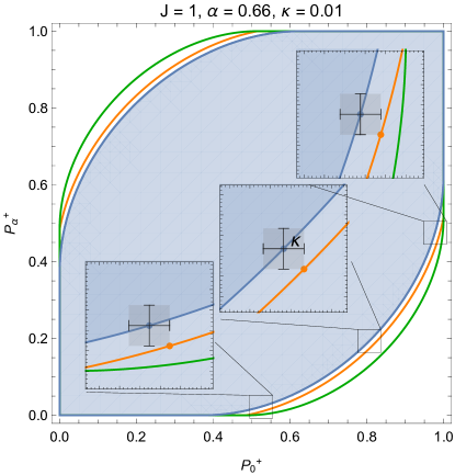
Figure 3: The quantum set $\mathcal{Q}_{J,a}$, the boundary of the set with error $\kappa$ (orange line) and the boundary of the smallest relaxed quantum set $\mathcal{Q}_{J,a}^{\delta}$ such that it includes the previous error set given by $\kappa$. The plot illustrates that $\mathcal{Q}_{J,a}^{\delta}$ always contains the set given by the error $\kappa$.

Relaxed classical set. Suppose now that the experimental error $\delta$ is of such a type that it could in principle be anticipated by an eavesdropper, such that there are more classical strategies available to her. We denote such epistemic error by $\varepsilon$, and characterise the set of classical correlations $\mathcal{C}^{\varepsilon}_{J,\alpha}$ accounting for this uncertainty. As in VanHimbeeck2017 , we define the relaxed classical set in terms of its quantum equivalent, with the additional assumption of deterministic outcomes:

$$\mathcal{C}_{J,\alpha}^{\varepsilon}= \left\{\mathbf{E}=\sum_{\lambda}p(\lambda)\mathbf{E}_{\lambda}\,\,\left|\,\,\mathbf{E}_{\lambda}\in\mathcal{Q}_{J_{\lambda},\alpha},\right.\right.$$

$$\;\left.\left.\sum_{\lambda:J_{\lambda}\leq J}p(\lambda)\geq 1-\varepsilon,\mathbf{E}_{\lambda}\in\{\pm 1\}\times\{\pm 1\}\right.\right\}.$$ (26)

Suppose that $J$ and $\alpha$ are such that $\mathcal{C}_{J,\alpha}$ is not the full square, $(\pm 1,\mp 1)\not\in\mathcal{C}_{J,\alpha}$. Then for all $\lambda$ with $J_{\lambda}\leq J$, we have $|E_{1|\lambda}-E_{2|\lambda}|=0$, and so all $\mathbf{E}^{\varepsilon}\in\mathcal{C}_{J,\alpha}^{\varepsilon}$ satisfy

$$|E^{\varepsilon}_{1}-E^{\varepsilon}_{2}|\leq\sum_{\lambda}p(\lambda)|E_{1|\lambda}-E_{2|\lambda}|\leq 2\varepsilon.$$ (27)

Conversely, suppose that $\mathbf{E}^{\varepsilon}$ satisfies Eq. (27). Consider the case $E_{1}^{\varepsilon}\leq E_{2}^{\varepsilon}$ (the other case can be treated analogously). In this case, it is geometrically clear that the line starting at the corner $(-1,1)$ which crosses $\mathbf{E}^{\varepsilon}$ hits the diagonal at some point $(E,E)$ with $-1\leq E\leq 1$. In other words, $\mathbf{E}^{\varepsilon}=\kappa(-1,1)+(1-\kappa)(E,E)$ for some $\kappa\in[0,1]$. From this, we obtain $\kappa=\frac{1}{2}(E_{2}^{\varepsilon}-E_{1}^{\varepsilon})\leq\varepsilon$, and so $E^{\varepsilon}\in\mathcal{C}_{J,\alpha}^{\varepsilon}$, since $(E,E)$ is a convex combination of the deterministic correlations $(\pm 1,\pm 1)$.

In summary, inequality (27) characterizes $\mathcal{C}_{J,\alpha}^{\varepsilon}$ exactly.

VI Calculating $H^{\star}_{0,0,\alpha}$

Here, we point out an equivalence between formulating the optimisation problem in Eq. (9) and the one presented in (van2019correlations, ), in order to use the algorithm presented in (van2019correlations, , Sec. 3.3) to find a numerical solution to our optimisation problem. In particular, the equivalence holds for the no-errors case (setting $\varepsilon=\omega=0$ in Eq. (9)), or (in the terminology of (van2019correlations, )) no max-average assumption. Under these cases, the only difference between formulating both optimisation problems is on how the set of allowed quantum correlations is defined. In our case, we have

$$\mathcal{Q}_{J,\alpha}:=\{\textbf{E}|E_{1}={\mathrm{Tr}}(\rho_{1}M),\,E_{2}={\mathrm{Tr}}(U_{\alpha}\rho_{1}U_{\alpha}^{\dagger}M)\}.$$

Meanwhile, in their case, the set of quantum correlations is defined as

$$\mathcal{Q}_{w_{\text{pk}}}:=\{(\textbf{E},\textbf{w})|\textbf{w}\leq\textbf{w}_{\text{pk}},\,E_{x}={\mathrm{Tr}}(\rho_{x}M),\,{\mathrm{Tr}}(\rho_{x}\mathcal{O})\leq w_{x}\},$$

where $x=\{1,2\}$, $\mathcal{O}$ is some energy operator, and $w_{1},w_{2}$ gives an upper bound on the energy peak (i.e. a “max-peak” assumption). In both cases, the set of correlations is characterised by the overlap between quantum states. In particular, we have the inequality

$$\frac{1}{2}\left(\sqrt{1+E_{1}}\sqrt{1+E_{2}}+\sqrt{1-E_{1}}\sqrt{1-E_{2}}\right)$$

$$\geq\left\{\begin{matrix}\cos(J\alpha)&\mbox{if}&|J\alpha|<\frac{\pi}{2}\\ 0&\mbox{if}&|J\alpha|\geq\frac{\pi}{2}\end{matrix}\right.,$$

whilst, in (van2019correlations, ), they have

$$\frac{1}{2}\left(\sqrt{1+E_{1}}\sqrt{1+E_{2}}+\sqrt{1-E_{1}}\sqrt{1-E_{2}}\right)$$

$$\geq\sqrt{1-w_{1}}\sqrt{1-w_{2}}-\sqrt{w_{1}}\sqrt{w_{2}}.$$

In our case, in order to calculate $H^{\star}_{0,0,\alpha}$, one can perform the algorithm in (van2019correlations, , Sec. 3.3) by setting some $w_{1}=w_{2}=w_{\text{pk}}$ such that $\cos(J\alpha)=1-2w_{\text{pk}}$. A numerical study on the amount of randomness is beyond the scope of this manuscript. Nonetheless, the curious reader may be referred to Figure $5$(b) of van2019correlations for an instance of $H^{\star}_{0,0,\alpha}$, for some given $J$ and $\alpha$ fulfilling the constraints.

VII Bounding $H^{\star}_{\varepsilon,\omega,\alpha}$

Note that we have $\mathcal{Q}_{J,\alpha}=\mathcal{Q}_{J,-\alpha}$, and thus $\mathcal{Q}_{J,\alpha}^{\omega}=\mathcal{Q}_{J,-\alpha}^{\omega}$ and $H^{\star}_{\varepsilon,\omega,\alpha}=H^{\star}_{\varepsilon,\omega,-\alpha}$. Thus, it is sufficient to consider the case $\alpha>0$ in this section.

The relaxed quantum and classical sets play a role for characterising imperfect protocols, in which we may want to consider types of error introduced into our setup, whereby our assumption on $J$ may fail. First, we have $\varepsilon$-type error, which can be thought of approximately as epistemic uncertainty of the experimenters; there may be additional variables $\lambda$ to which they may not have access (but to which Eve may), such that $\lambda$ describes exactly when our assumption fails. Second, we have $\omega$-type error, which can be thought of as genuine, ontic randomness, such as that introduced by sending coherent states, for which the photon number (and the spin) can only be described probabilistically. This type of randomness cannot be described by any classical side-information that Eve may hold, and even she could never predict when the assumption fails. The amount of randomness $H^{\star}=H^{\star}_{\varepsilon,\omega,\alpha}$ that can be certified using our setup is thus affected by the room that we wish to grant for these types of experimental errors.

To bound the certified randomness given such errors, let $\{p(\lambda),\mathbf{E}^{\lambda}\}$ be a minimizing ensemble for $H_{\varepsilon,\omega,\alpha}^{\star}$, i.e.

$$H_{\varepsilon,\omega,\alpha}^{\star} = \sum_{\lambda}p(\lambda)H(\mathbf{E}^{\lambda}),$$ (30)

$$\sum_{\lambda:\mathbf{E}^{\lambda}\in\mathcal{Q}_{J,\alpha}^{\omega}}p(\lambda)\geq 1-\varepsilon,$$

$$\sum_{\lambda}p(\lambda)\mathbf{E}^{\lambda}=\mathbf{E}.$$

Then, for all $\varepsilon^{\prime}\geq\varepsilon$, we trivially have

$$\sum_{\lambda:\mathbf{E}^{\lambda}\in\mathcal{Q}_{J,\alpha}^{\omega}}p(\lambda)\geq 1-\varepsilon\geq 1-\varepsilon^{\prime},$$

and so the ensemble $\{p(\lambda),\mathbf{E}^{\lambda}\}$ satisfies the conditions that define the optimisation problem for $H^{\star}_{\varepsilon^{\prime},\omega,\alpha}$. Consequently,

$$H^{\star}_{\varepsilon^{\prime},\omega,\alpha}\leq H^{\star}_{\varepsilon,\omega,\alpha}.$$ (31)

Similarly, $\omega^{\prime}\geq\omega$ implies $\mathcal{Q}_{J,\alpha}^{\omega^{\prime}}\supseteq\mathcal{Q}_{J,\alpha}^{\omega}$, and so

$$\sum_{\lambda:\mathbf{E}^{\lambda}\in\mathcal{Q}_{J,\alpha}^{\omega^{\prime}}}p(\lambda)\geq\sum_{\lambda:\mathbf{E}^{\lambda}\in\mathcal{Q}_{J,\alpha}^{\omega}}p(\lambda)\geq 1-\varepsilon,$$

hence $\{p(\lambda),\mathbf{E}^{\lambda}\}$ is also a candidate ensemble for $H^{\star}_{\varepsilon,\omega^{\prime},\alpha}$. It follows that

$$H^{\star}_{\varepsilon,\omega^{\prime},\alpha}\leq H^{*}_{\varepsilon,\omega,\alpha}.$$ (32)

In particular, Eqs. (31) and (32) imply the following result:

Lemma 1.

Both types of error $\varepsilon,\omega>0$ decrease the number of certified random bits:

$$H^{\star}_{\varepsilon,\omega,\alpha}\leq H^{\star}_{0,0,\alpha}.$$

To obtain inequalities in the converse direction, the following intermediate result will be useful. It is motivated by the Taylor expansion

$$\arccos\left((1-\omega)^{2}\cos x\right)=x+2\omega\cot x+\mathcal{O}(\omega^{2}),$$

which also shows that the constant factor appearing in front of $\omega$ in the following lemma cannot be improved.

Lemma 2.

Suppose that $0\leq\omega\leq 1$ and $0\leq x\leq\frac{\pi}{2}$. Then

$$(1-\omega)^{2}\cos x\geq\cos_{*}(x+2\omega\cot x),$$

where

$$\cos_{*}(t):=\left\{\begin{array}[]{cl}\cos t&\mbox{if }0\leq t\leq\frac{\pi}{2}\\ 0&\mbox{otherwise}.\end{array}\right.$$

Proof.

If $x+2\omega\cot x\geq\frac{\pi}{2}$, then the inequality is trivially true, since the left-hand side is non-negative. Thus, it is sufficient to consider the case $x+2\omega\cot x<\frac{\pi}{2}$. For every fixed $x$, consider the function $g:[0,1]\to\mathbb{R}$, given by

$$g(\omega):=\sin(x+2\omega\cot x)-(1-\omega)\sin x.$$

We have $g(0)=0$ and

$$g^{\prime}(\omega)=2\cos(x+2\omega\cot x)\cot x+\sin x\geq 0.$$

Therefore, $g(\omega)\geq 0$ for all $\omega\in[0,1]$. Now consider

$$f(\omega):=(1-\omega)^{2}\cos x-\cos(x+2\omega\cot x).$$

We have $f(0)=0$ and

$$f^{\prime}(\omega)=2(\cot x)g(\omega)\geq 0.$$

Thus $f(\omega)\geq 0$ for all $\omega\in[0,1]$. ∎

Lemma 3.

For $0\leq\omega\leq 1$, we have the set inclusion

$$\mathcal{Q}_{J,\alpha}^{\omega}\subseteq\mathcal{Q}_{J,\alpha+2\omega\cot(J\alpha)/J}.$$

Proof.

If $J\alpha+2\omega\cot(J\alpha)>\frac{\pi}{2}$, then $\mathcal{Q}_{J,\alpha+2\omega\cot(J\alpha)/J}=[-1,1]^{2}$, and the claim is trivially true. Thus, we may assume that $J\alpha+2\omega\cot(J\alpha)\leq\frac{\pi}{2}$. Suppose that $\mathbf{E}\in\mathcal{Q}_{J,\alpha}^{\omega}$, then there exist $\mathbf{E}^{J}\in\mathcal{Q}_{J,\alpha}$ and $\mathbf{E}^{\prime}\in[-1,1]^{2}$ such that

$$\mathbf{E}=(1-\omega)\mathbf{E}^{J}+\omega\mathbf{E}^{\prime}.$$

Now we use the fact the the functions $x\mapsto\sqrt{1-x}$ and $x\mapsto\sqrt{1+x}$ are concave and non-negative on $[-1,1]$:

$$\frac{1}{2}\left(\sqrt{1+E_{1}}\sqrt{1+E_{2}}+\sqrt{1-E_{1}}\sqrt{1-E_{2}}\right)$$

$$= \frac{1}{2}\left(\sqrt{1+(1-\omega)E_{1}^{J}+\omega E^{\prime}_{1}}\sqrt{1+(1-\omega)E_{2}^{J}+\omega E^{\prime}_{2}}\right.$$

$$\left.+\sqrt{1-\left((1-\omega)E_{1}^{J}+\omega E^{\prime}_{1}\right)}\sqrt{1-\left((1-\omega)E_{2}^{J}+\omega E^{\prime}_{2}\right)}\right)$$

$$\geq \frac{1}{2}\left[\left((1-\omega)\sqrt{1+E_{1}^{J}}+\omega\sqrt{1+E^{\prime}_{1}}\right)\times\right.$$

$$\quad\times\left((1-\omega)\sqrt{1+E_{2}^{J}}+\omega\sqrt{1+E^{\prime}_{2}}\right)$$

$$\quad+\left((1-\omega)\sqrt{1-E_{1}^{J}}+\omega\sqrt{1-E^{\prime}_{1}}\right)\times$$

$$\left.\quad\times\left((1-\omega)\sqrt{1-E_{2}^{J}}+\omega\sqrt{1-E^{\prime}_{2}}\right)\right]$$

$$\geq \frac{1}{2}\left[\sqrt{1+E_{1}^{J}}\sqrt{1+E_{2}^{J}}+\sqrt{1-E_{1}^{J}}\sqrt{1-E_{2}^{J}}\right](1-\omega)^{2}$$

$$\geq (1-\omega)^{2}\cos(J\alpha)$$

$$\geq \cos_{*}(J\alpha+2\omega\cot(J\alpha)),$$

where we have used Lemma 2 in the final step. Therefore, $\mathbf{E}\in\mathcal{Q}_{J,\alpha+2\omega\cot(J\alpha)/J}$, and the claim follows. ∎

Now recall Eqs. (30), (30) and (30) which are satisfied by the minimizing ensemble $\{p(\lambda),\mathbf{E}^{\lambda}\}$ for $H^{\star}_{\varepsilon,\omega,\alpha}$. In particular, Eq. (30) and Lemma 3 imply that

$$\sum_{\lambda:\mathbf{E}^{\lambda}\in\mathcal{Q}_{J,\alpha+2\omega\cot(J\alpha)/J}}p(\lambda)\geq\sum_{\lambda:\mathbf{E}^{\lambda}\in\mathcal{Q}_{J,\alpha}^{\omega}}p(\lambda)\geq 1-\varepsilon,$$ (34)

and so Eqs. (30) and (34) show that $\{p(\lambda),\mathbf{E}^{\lambda}\}$ is a candidate ensemble for $H^{\star}_{J,\alpha+2\omega\cot(J\alpha)/J}$. This proves the following corollary:

Corollary 1.

We have

$$H^{\star}_{\varepsilon,\omega,\alpha}\geq H^{\star}_{\varepsilon,0,\alpha+2\omega\cot(J\alpha)/J}.$$

Finally, we would like to obtain an inequality that tells us what happens if replace a finite value of $\varepsilon$ by zero. To this end, we will use an inverse concavity property (see e.g. nielsen2010 ) of Shannon entropy

$$H(q)=H(q_{1},\ldots,q_{n}):=-\sum_{i=1}^{n}q_{i}\log q_{i}.$$

If we have $n$ probability distributions $p^{(i)}=(p^{(i)}_{1},\ldots,p^{(i)}_{m})$ (vectors with non-negative entries summing to unity), and another probability distribution $q=(q_{1},\ldots,q_{n})$, then

$$H\left(\sum_{i=1}^{n}q_{i}p^{(i)}\right)\leq\sum_{i=1}^{n}q_{i}H(p^{(i)})+H(q).$$

In the notation of the main text, the corresponding entropy of a correlation $\mathbf{E}$ therefore satisfies

$$H(t\mathbf{E}+(1-t)\mathbf{E}^{\prime}) \leq tH(\mathbf{E})+(1-t)H(\mathbf{E}^{\prime})$$ (35)

$$-t\log t-(1-t)\log(1-t)$$

for all $0\leq t\leq 1$ (with the convention $0\log 0:=0$). To see this, use for example that $H(\mathbf{E})=\frac{1}{2}\sum_{x}H(p^{(x)}_{\mathbf{E}})$, where $p^{(x)}_{\mathbf{E}}$ is the binary distribution with probabilities $\frac{1\pm E_{x}}{2}$. We will use this to prove the following result:

Lemma 4.

For every $0\leq\varepsilon,\omega<1$, we have

$$H^{\star}_{\varepsilon,\omega,\alpha}\geq H^{\star}_{0,\varepsilon+\omega,\alpha}+\log(1-\varepsilon)-\frac{\varepsilon\log(2/\varepsilon)}{1-\varepsilon},$$

with the convention that $0\log(2/0):=0$.

Proof.

Consider again a minimizing ensemble for $H^{\star}_{\varepsilon,\omega,\alpha}$, satisfying Eqs. (30)–(30). Such choice of ensemble also entails a definition of a set of “hidden variables” $\Lambda\ni\lambda$. Define the subset $\Lambda_{\omega}:=\{\lambda\in\Lambda\,\,|\,\,\mathbf{E}^{\lambda}\in\mathcal{Q}_{J,\alpha}^{\omega}\}$, then

$$t:=1-\sum_{\lambda\in\Lambda_{\omega}}p(\lambda)\leq\varepsilon.$$

Therefore, $\mathbf{E}^{J}:=\sum_{\lambda\in\Lambda_{\omega}}\frac{p(\lambda)}{1-t}\mathbf{E}^{\lambda}\in\mathcal{Q}_{J,\alpha}^{\omega}$ because $\mathcal{Q}_{J,\alpha}^{\omega}$ is convex. Now, if $t=0$, let $\mathbf{E}^{\prime}$ be an arbitrary correlation, while for $t>0$, set $\mathbf{E}^{\prime}:=\sum_{\lambda\not\in\Lambda_{\omega}}\frac{p(\lambda)}{t}\mathbf{E}^{\lambda}$, then $\mathbf{E}=(1-t)\mathbf{E}^{J}+t\mathbf{E}^{\prime}$. For all $\lambda\in\Lambda_{\omega}$, set $q(\lambda):=p(\lambda)/(1-t)$ and $\mathbf{F}^{\lambda}:=(1-t)\mathbf{E}^{\lambda}+t\mathbf{E}^{\prime}$. Then direct calculation shows that

$$\sum_{\lambda\in\Lambda_{\omega}}q(\lambda)\mathbf{F}^{\lambda}=(1-t)\mathbf{E}^{J}+t\mathbf{E}^{\prime}=\mathbf{E}.$$

Since $\mathbf{E}^{\lambda}\in\mathcal{Q}_{J,\alpha}^{\omega}$, there exist correlations $\mathbf{E}^{\lambda,J}\in\mathcal{Q}_{J,\alpha}$ and $\mathbf{E}^{\lambda,\bullet}\in[-1,1]^{2}$ such that $\mathbf{E}^{\lambda}=(1-\omega)\mathbf{E}^{\lambda,J}+\omega\mathbf{E}^{\lambda,\bullet}$. Thus

$$\mathbf{F}^{\lambda} = (1-t)\mathbf{E}^{\lambda}+t\mathbf{E}^{\prime}$$

$$= (1-t)(1-\omega)\mathbf{E}^{\lambda,J}+(1-t)\omega\mathbf{E}^{\lambda,\bullet}+t\mathbf{E}^{\prime}$$

$$\in \mathcal{Q}_{J,\alpha}^{t+\omega-t\omega}\subseteq\mathcal{Q}_{J,\alpha}^{t+\omega}\subseteq\mathcal{Q}_{J,\alpha}^{\varepsilon+\omega}.$$

It follows that $\{q(\lambda),\mathbf{F}^{\lambda}\}_{\lambda\in\Lambda_{\omega}}$ is a candidate ensemble for $H^{\star}_{0,\varepsilon+\omega,\alpha}$. Using furthermore that $H(\mathbf{E}^{\prime})\leq\log 2$, we obtain

$$H^{\star}_{0,\varepsilon+\omega,\alpha} \leq \sum_{\lambda\in\Lambda_{\omega}}q(\lambda)H(\mathbf{F}^{\lambda})$$

$$\leq \sum_{\lambda\in\Lambda}q(\lambda)H\left((1-t)\mathbf{E}^{\lambda}+t\mathbf{E}^{\prime}\right)$$

$$\leq \sum_{\lambda\in\Lambda}\frac{p(\lambda)}{1-t}\left((1-t)H(\mathbf{E}^{\lambda})+tH(\mathbf{E}^{\prime})\right.$$

$$\left.\qquad\qquad-t\log t-(1-t)\log(1-t)\right)$$

$$= \sum_{\lambda\in\Lambda}p(\lambda)H(\mathbf{E}^{\lambda})+\frac{H(\mathbf{E}^{\prime})}{1-t}-\frac{t\log t}{1-t}-\log(1-t)$$

$$\leq H^{\star}_{\varepsilon,\omega,\alpha}+\frac{t\log(2/t)}{1-t}-\log(1-t).$$

Using finally that $t\leq\varepsilon$ completes the proof. ∎

Applying Lemma 4 and Corollary 1 in succession shows the following:

Corollary 2.

If $\varepsilon,\omega\in[0,1)$, then

$$H^{\star}_{\varepsilon,\omega,\alpha}\geq H^{\star}_{0,0,\alpha+2(\varepsilon+\omega)\cot(J\alpha)/J}+\log(1-\varepsilon)-\frac{\varepsilon\log(2/\varepsilon)}{1-\varepsilon}.$$

VIII Proof that $\mathcal{Q}_{J}\subseteq\mathcal{R}_{J}$

Since $\mathcal{R}_{J}$ is a convex set, it is sufficient to show that extremal correlations of $\mathcal{Q}_{J}$ are contained in it. That is, we can disregard shared randomness and consider a fixed POVM $\{M_{b}\}_{b}$ and an arbitrary, normalized pure state

$$\ket{\phi}=\sum_{j=-J}^{J}\phi_{j}\ket{\psi_{j}},$$

where $\ket{\psi_{j}}\in\mathcal{H}_{j}$ is normalised and $\phi_{j}=\innerproduct{\psi_{j}}{\phi}$. We choose an orthonormal basis for $\mathcal{H}$, such that every $\ket{\psi_{k}}$ is an element of this basis, and we calculate the probabilities in this basis:

$$P(b|\alpha) = {\mathrm{tr}}[U_{\alpha}\outerproduct{\phi}{\phi}U_{\alpha}^{\dagger}M_{b}]$$

$$= \sum_{j,j^{\prime}=-J}^{J}\phi_{j}\phi_{j^{\prime}}^{*}e^{ij\alpha}M^{b}_{jj^{\prime}}e^{-ij^{\prime}\alpha}$$

$$= \sum_{l=-2J}^{2J}\sum_{\begin{matrix}-J\leq j,j^{\prime}\leq J\!:\\ j\!-\!j^{\prime}=l\end{matrix}}\phi_{j}\phi_{j^{\prime}}^{*}M^{b}_{jj^{\prime}}e^{i(j-j^{\prime})\alpha}$$

$$= \sum_{l=-2J}^{2J}a_{l}e^{il\alpha},$$

where we have defined the coefficients

$$a_{l}=\sum_{\begin{matrix}-J\leq j,j^{\prime}\leq J\!:\\ j\!-\!j^{\prime}=l\end{matrix}}\phi_{j}\phi_{j^{\prime}}^{*}M^{b}_{jj^{\prime}},$$

for $-J\leq l\leq J$, and $M^{b}_{jj^{\prime}}:=\langle j^{\prime}|M_{b}|j\rangle$. The coefficients have the property

$$a_{l} = \sum_{\begin{matrix}-J\leq j,j^{\prime}\leq J\\ j\!-\!j^{\prime}=l\end{matrix}}\phi_{j}\phi_{j^{\prime}}^{*}M^{b}_{jj^{\prime}}$$

$$= \sum_{\begin{matrix}-J\leq j,j^{\prime}\leq J\\ j\!-\!j^{\prime}=l\end{matrix}}\left(\phi_{j}^{*}\phi_{j^{\prime}}\right)^{*}\left(M^{b}_{j^{\prime}j}\right)^{*}=a^{*}_{-l},$$

which we can use to write

$$P(b|\alpha) = \sum_{l=-2J}^{2J}a_{l}(\cos(l\alpha)+i\sin(l\alpha))$$

$$= a_{0}+\sum_{l=1}^{2J}\left(2\real(a_{l})\cos(l\alpha)-2\imaginary(a_{l})\sin(l\alpha)\right),$$

By observing that this is exactly of the form (10), we conclude that $\mathcal{Q}_{J}\subseteq\mathcal{R}_{J}$, and thus also $\mathcal{Q}_{J,\alpha}\subseteq\mathcal{R}_{J,\alpha}$.

IX Proof that $\mathcal{Q}_{1/2}=\mathcal{R}_{1/2}$

In this section we will show that for a $J=1/2$ system, not only do the sets $\mathcal{Q}_{1/2,\alpha}$ and $\mathcal{R}_{1/2,\alpha}$ coincide, but in fact every rotation box can be simulated by a quantum model, i.e. $\mathcal{Q}_{1/2}=\mathcal{R}_{1/2}$.

Rotation boxes. We will start our discussion by giving a characterisation of the convex set $\mathcal{R}_{1/2}=\{P(+1|\alpha)|\alpha\mapsto P(+1|\alpha)\;\mbox{as in}\;(\ref{SBs})\}$. Hence, every $J=1/2$ rotation box is described by probability distributions of the form

$$P(+1|\alpha)=c_{0}+c_{1}\cos{\alpha}+s_{1}\sin\alpha,$$ (36)

where $c_{0},c_{1},s_{1}\in\mathbb{R}$, s.t. $0\leq P(1|\alpha)\leq 1\,\forall\alpha$.

To find conditions for $c_{0}$, we integrate $0\leq P(+1|\alpha)\leq 1$ from $0$ to $2\pi$ and divide the inequality by $2\pi$. This gives us the condition

$$0\leq c_{0}\leq 1.$$ (37)

Furthermore, from

$$0\leq P(1|0)=c_{0}+c_{1}\leq 1$$

and

$$0\leq P\left(1|\pi\right)=c_{0}-c_{1}\leq 1,$$

we can find equivalently the two conditions

$$|c_{1}|\leq c_{0}$$ (38)

and

$$c_{0}\leq 1-|c_{1}|.$$ (39)

Using similar reasoning, we also find

$$|s_{1}|\leq c_{0}$$ (40)

and

$$c_{0}\leq 1-|s_{1}|.$$ (41)

If we chose $s_{1}=c_{1}=0$, then $P(+1|\alpha)$ is a constant function, and, as long as $0\leq c_{0}\leq 1$, it gives valid probabilities. In the case where only $s_{1}=0$, $P(+1|\alpha)$ has its extreme values at $\alpha=n\pi$, $n\in\mathbb{Z}$; therefore $P(+1|\alpha)$ yields valid probabilities iff conditions (38) and (39) are met. In the case where $c_{1}=0$, $P(+1|\alpha)$ has its extreme values at $\alpha=(2n+1)/2$, $n\in\mathbb{Z}$; therefore $P(+1|\alpha)$ gives valid probabilities iff conditions (40) and (41) are satisfied.

Next, we assume $s_{1}\neq 0$ and $c_{1}\neq 0$. To find the extreme value of $P(+1|\alpha)$, we calculate

$$\frac{d(P(+1|\alpha))}{d\alpha}=-c_{1}\sin\alpha+s_{1}\cos\alpha$$

and we set $d(P(+1|\alpha))/d\alpha=0$, which gives us

$$\frac{\sin\alpha}{\cos\alpha}=\tan\alpha=\frac{s_{1}}{c_{1}},$$

since $c_{1}\neq 0$ we find that $P(+1|\alpha)$ has its extreme values at

$$\alpha=\tan^{-1}\left(\frac{s_{1}}{c_{1}}\right)+\pi n,$$

where $n\in\mathbb{Z}$.

Next, we will distinguish between the two cases, where $n$ is odd or even. We start with $n$ being even. Then we have the condition

$$0 \leq P\left(1\left|\tan^{-1}\left(\frac{s_{1}}{c_{1}}\right)+\pi n\right.\right)$$

$$= c_{0}+c_{1}\cos\left(\tan^{-1}\left(\frac{s_{1}}{c_{1}}\right)\right)+s_{1}\sin\left(\tan^{-1}\left(\frac{s_{1}}{c_{1}}\right)\right)$$

$$= c_{0}+c_{1}\frac{1}{\sqrt{\left(\frac{s_{1}}{c_{1}}\right)^{2}+1}}+s_{1}\frac{s_{1}}{c_{1}\sqrt{\left(\frac{s_{1}}{c_{1}}\right)^{2}+1}}$$

$$= c_{0}+\frac{(c_{1})^{2}+(s_{1})^{2}}{c_{1}\sqrt{\left(\frac{s_{1}}{c_{1}}\right)^{2}+1}}$$

$$= c_{0}+\frac{(c_{1})^{2}+(s_{1})^{2}}{\frac{c_{1}}{|c_{1}|}\sqrt{(s_{1})^{2}+(c_{1})^{2}}}$$

$$= c_{0}+\mbox{sgn}(c_{1})\frac{(c_{1})^{2}+(s_{1})^{2}}{\sqrt{(s_{1})^{2}+(c_{1})^{2}}}\leq 1.$$

For $n$ being odd we have

$$0 \leq P\left(1\left|\frac{1}{\omega}\left(\tan^{-1}\left(\frac{s_{1}}{c_{1}}\right)+\pi n\right)\right.\right)$$

$$= c_{0}-c_{1}\cos\left(\tan^{-1}\left(\frac{s_{1}}{c_{1}}\right)\right)-s_{1}\sin\left(\tan^{-1}\left(\frac{s_{1}}{c_{1}}\right)\right)$$

$$= c_{0}-\mbox{sgn}(c_{1})\frac{(c_{1})^{2}+(s_{1})^{2}}{\sqrt{(s_{1})^{2}+(c_{1})^{2}}}\leq 1.$$

Again, by combining the last two inequalities, we find equivalently the two conditions

$$\frac{(c_{1})^{2}+(s_{1})^{2}}{\sqrt{(c_{1})^{2}+(s_{1})^{2}}}\leq c_{0}$$ (42)

and

$$c_{0}\leq 1-\frac{(c_{1})^{2}+(s_{1})^{2}}{\sqrt{(c_{1})^{2}+(s_{1})^{2}}}.$$ (43)

So, in the case $s_{1}\neq 0$ and $c_{1}\neq 0$, $P(+1|\alpha)$ gives valid probabilities for all $\alpha$ iff conditions (42) and (43) hold.

From (42) it follows that

$$(c_{1})^{2}+(s_{1})^{2}\leq(c_{0})^{2}.$$ (44)

The converse is not true, since (42) tells us that $c_{0}$ must be larger than 0, while (44) only tells us that $c_{0}\neq 0$, but we do not obtain any information about whether $c_{0}$ is positive or negative. However, the condition $c_{0}>0$ together with (44) is equivalent to (42). Similarly, (43) gives us

$$(c_{1})^{2}+(s_{1})^{2}\leq(1-c_{0})^{2},$$ (45)

which, similarly, is only equivalent to (43) if we additionally demand that $c_{0}<1$.

Now, we come back to the general case, where we do not make any assumption about $s_{1}$ and $c_{1}$, as long as $0\leq P(+1|\alpha)\leq 1$. In this case, we find that (44) and $0<c_{0}$ together imply (38) and (40), whilst condition (45) together with $c_{0}<1$ implies (39) and (41). We notice that we can replace the condition $0<c_{0}$ by $0\leq c_{0}$, since it has no consequence for condition (44), if $c_{1}\neq 0$ or $s_{1}\neq 0$. Similarly, we can replace condition $c_{0}<1$ by $c_{0}\leq 1$.

Let us summarise our findings so far. Namely, $P(+1|\alpha)$ gives valid probabilities iff the three conditions (37)(44) and (45) are met. However, for $0\leq c_{0}\leq 1/2$ we find (44)$\Rightarrow$(45), since

$$(1-c_{0})^{2}\geq\frac{1}{4}\geq(c_{0})^{2}\geq(c_{1})^{2}+(s_{1})^{2}.$$

Similarly, for $1/2\leq c_{0}\leq 1$ we find (45)$\Rightarrow$(44), since

$$(c_{0})^{2}\geq 1/4\geq(1-c_{0})^{2}\geq(c_{1})^{2}+(s_{1})^{2}.$$

This allows us to write the set $\mathcal{R}_{1/2}$ in the neat form:

$$\mathcal{R}_{1/2} = \bigg{\{}P(+1|\alpha)\left|0\leq c_{0}\leq 1;\right.$$

$$\mbox{if}\,\frac{1}{2}<c_{0},\,\mbox{then}\,(c_{0})^{2}\geq(c_{1})^{2}+(s_{1})^{2};$$

$$\mbox{if}\,c_{0}\leq\frac{1}{2},\,\mbox{then}\,(1-c_{0})^{2}\geq(c_{1})^{2}+(s_{1})^{2}\bigg{\}}.$$

The convexity of $\mathcal{R}_{1/2}$ follows immediately from the fact that the set of probabilities is convex and that a convex combination of functions of the form $c_{0}+c_{1}\cos\alpha+s_{1}\sin\alpha$ gives again a function of the same form.

Furthermore, the set $\mathcal{R}_{1/2}$ is isomorphic to the subset $\mathcal{A}\subset\mathbb{R}^{3}$, given by

$$\mathcal{R}_{1/2} \cong \left\{\begin{pmatrix}(x&y&z)\end{pmatrix}^{T}\left|0\leq x\leq 1;\right.\right.$$

$$\mbox{if}\,x\leq\frac{1}{2},\mbox{then}\,x^{2}\geq y^{2}+z^{2};$$

$$\left.\mbox{if}\,\frac{1}{2}<x,\mbox{then}\,(1-x)^{2}\geq y^{2}+z^{2}\right\}$$

$$= \mathcal{A}\subset\mathbb{R}^{3}.$$

Figure 4: $\mathcal{R}_{1/2}=\mathcal{Q}_{1/2}$ as a convex set.

The isomorphism $\varphi:S\rightarrow\mathcal{A}$ is given by

$$\varphi(P(+1|\alpha))=\begin{pmatrix}c_{0}\\ c_{1}\\ s_{1}\end{pmatrix},$$

which is clearly linear and therefore affine – that is, $\mathcal{A}$ inherits its convex properties form $\mathcal{R}_{1/2}$ and vice versa.

We will now find the extreme points of the set $\mathcal{A}$, and therefore the extreme points of $\mathcal{R}_{1/2}$. Let us start with the point $\begin{pmatrix}0&0&0\end{pmatrix}^{T}$. Let $\lambda\in(0,1)$ and $a,b\in\mathcal{A}$, then

$$\lambda a+(1-\lambda)b=\begin{pmatrix}\lambda x_{a}+(1-\lambda)x_{b}\\ \lambda y_{a}+(1-\lambda)y_{b}\\ \lambda z_{a}+(1-\lambda)z_{b}\end{pmatrix}=\begin{pmatrix}0\\ 0\\ 0\end{pmatrix}.$$

From $\lambda x_{a}+(1-\lambda)x_{b}=0$ it follows that $x_{a}=x_{b}=0$. This implies though that $y_{a}=y_{b}=z_{a}=z_{b}=0$, and therefore $\begin{pmatrix}0&0&0\end{pmatrix}^{T}$ is an extreme point. Similarly, one can find that $\begin{pmatrix}1&0&0\end{pmatrix}^{T}$ is an extreme point as well.

Next, let us consider all points for a fixed $0<x\leq 1/2$. For these points the condition

$$y^{2}+z^{2}\leq x^{2},$$

defines a circle area with radius $x$. Clearly, every interior point of the circle area can be written as a convex combination, that is all points $\begin{pmatrix}x&y&z\end{pmatrix}^{T}$ satisfying $y^{2}+z^{2}<x^{2}$ and $0<x\leq 1/2$ are not extreme points. Similarly, one can show that points satisfying $y^{2}+z^{2}<(1-x)^{2}$ and $1/2<x<1$ are also not extreme points.

We still have to check though which of the points satisfying $y^{2}+z^{2}=x^{2}$ and $0<x\leq 1/2$, and which of the points satisfying $y^{2}+z^{2}=(1-x)^{2}$ and $1/2<x<1$ are extreme.

Let us consider a point $a=\begin{pmatrix}1/2&y&z\end{pmatrix}^{T}$ that satisfies $y^{2}+z^{2}=1/4$ first. We will check that $a$ is an extreme point by showing, as before, that it cannot be written as a convex combination of any $b,c\in\mathcal{A}$, for $a\neq b$ and $a\neq c$. That is, $a$ cannot be written as

$$\begin{pmatrix}1/2\\ y\\ z\end{pmatrix}=\begin{pmatrix}\lambda x_{b}+(1-\lambda)x_{c}\\ \lambda y_{b}+(1-\lambda)y_{c}\\ \lambda z_{b}+(1-\lambda)z_{c}\end{pmatrix},$$

with $0<\lambda<1$. We assume, without loss of generality, that $x_{b}\leq x_{c}$.

First, let us choose $x_{c}=\frac{1}{2}$. Then we have

$$\lambda x_{b}+(1-\lambda)\frac{1}{2}=\frac{1}{2}\;\Leftrightarrow\;\lambda x_{b}=\lambda\frac{1}{2}\Leftrightarrow x_{b}=\frac{1}{2},$$

but then $a,b$ and $c$ are in a plane. All elements of $\mathcal{A}$ in this plane build up a circle area, where $a,b$ and $c$ are on the boundary of the circle area. Since the boundary of the circle area coincides with its extreme points, it follows that $a=b=c$.

Next, we choose that $x_{c}<1/2$. From $0\leq x_{b}\leq x_{c}<1/2$ we find

$$\frac{1}{2}=\lambda x_{b}+(1-\lambda)x_{c}\leq\lambda x_{c}<\frac{1}{2},$$

which is a contradiction.

We are left with the case that $1/2<x_{c}\leq 1$. For this case we find

$$\frac{1}{2}=\lambda x_{b}+(1-\lambda)x_{c}>x_{b}.$$

The two inequalities $1/2<x_{c}\leq 1$ and $0\leq x_{b}<1/2$ imply that

$$y_{c}^{2}+z_{c}^{2}<\frac{1}{4}$$

and

$$y^{2}_{b}+z^{2}_{b}<\frac{1}{4}.$$

That is, the projections of the points $b$ and $c$ into the plane $x=1/2$ are within the interior of the circle area. However, $a$ is by definition on the boundary of the circle, and therefore $a$ cannot be written as a convex combination of two other points $b,c\in\mathcal{A}$, so we also have a contradiction here. Thus, $a$ must be an extreme point.

To close this subsection, we will show that the extreme points we have found so far are the only extreme points of $\mathcal{A}$. We start by showing that a point $a$ satisfying $0<x_{a}<1/2$ and $y^{2}_{a}+z^{2}_{a}=x_{a}^{2}$ can be written as a convex combination of the point $\begin{pmatrix}0&0&0\end{pmatrix}^{T}$ and some point $b$, which satisfies $x_{b}=1/2$ and $y_{b}^{2}+z_{b}^{2}=1/4$. We have

$$a=\begin{pmatrix}x_{a}\\ y_{a}\\ z_{b}\end{pmatrix}=(1-2x_{a})\begin{pmatrix}0\\ 0\\ 0\end{pmatrix}+2x_{a}\begin{pmatrix}\frac{1}{2}\\ \frac{y_{a}}{2x_{a}}\\ \frac{z_{a}}{2x_{a}}\end{pmatrix}.$$

Obviously, $0<2x_{a}<1$ holds and

$$\left(\frac{y_{a}}{2x_{a}}\right)^{2}+\left(\frac{z_{a}}{2x_{a}}\right)^{2}=\left(\frac{y^{2}_{a}+z^{2}_{a}}{4x^{2}_{a}}\right)=\frac{x_{a}^{2}}{4x_{a}^{2}}=\frac{1}{4}.$$

Similarly, one can find that the point $a$ satisfying $1/2<x_{a}<1$ and $y^{2}_{a}+z^{2}_{a}=x_{a}^{2}$ can be written as a convex combination of the point $c=\begin{pmatrix}1&0&0\end{pmatrix}$ and the point $b=\begin{pmatrix}1/2&y_{a}/2(1-x_{a})&z_{a}/2(1-x_{a})^{T}\end{pmatrix}$, i.e. as

$$a=(1-\lambda)c+\lambda b,$$

where $\lambda=2(1-x_{a})$.

In summary, we have found that the extreme points $\partial_{\rm ext}\mathcal{A}$ of $\mathcal{A}$ are described by:

$$\partial_{\rm ext}\mathcal{A} = \left\{\begin{pmatrix}0\\ 0\\ 0\end{pmatrix},\begin{pmatrix}1\\ 0\\ 0\end{pmatrix},\left\{\left.\begin{pmatrix}\frac{1}{2}\\ y\\ z\end{pmatrix}\right|y^{2}+z^{2}=\frac{1}{4}\right\}\right\}$$

$$\cong \partial_{\rm ext}\mathcal{R}_{1/2}.$$

Rotation Boxes Simulated by Quantum Model. We now find quantum models for the extreme points of $\mathcal{R}_{1/2}$.

The extreme points $P(+1|\alpha)=1$ and $P(+1|\alpha)=0$ are just constant probability distributions and therefore can obviously be simulated by quantum theory. For example, consider $\ket{\phi_{\frac{1}{2}}}\in\mathcal{H}_{+\frac{1}{2}}$ and the measurment $\left\{P_{+}=\outerproduct{\phi_{+\frac{1}{2}}}{\phi_{+\frac{1}{2}}},P_{-}=\mathds{1}-P_{+}\right\}$. This yields the probability distribution

$$P(+1|\alpha) = \bra{\phi_{+\frac{1}{2}}}U^{\dagger}_{\alpha}P_{+}U_{\alpha}\ket{\phi_{+\frac{1}{2}}}$$

$$= \left|e^{i\frac{\alpha}{2}}\innerproduct{\phi_{+\frac{1}{2}}}{\phi_{+\frac{1}{2}}}\right|^{2}=1.$$

In similar fashion one can construct a quantum model for $P(+1|\alpha)=0$.

All other extreme points are of the form

$$P_{\tau}(+1|\alpha) = \frac{1}{2}+c_{1}^{\tau}\cos\alpha+s_{1}^{\tau}\sin\alpha$$ (46)

$$= \frac{1}{2}\left(1+\cos\alpha\cos\tau+\sin\alpha\sin\tau\right)$$

$$= \frac{1}{2}\left(1+\cos(\alpha-\tau)\right),$$

where we have used that we can write $c^{\tau}_{1}=(1/2)\cos\tau$ and $s_{1}^{\tau}=(1/2)\sin\tau$ such that $\left(c^{\tau}_{1}\right)^{2}+\left(s_{1}^{\tau}\right)^{2}=1/4$ is satisfied.

To find a quantum model for these probability distributions we define the state

$$\ket{\phi}=\frac{1}{\sqrt{2}}\left(\ket{\phi_{+\frac{1}{2}}}+\ket{\phi_{-\frac{1}{2}}}\right),$$

where $\ket{\phi_{\pm\frac{1}{2}}}\in\mathcal{H}_{\pm\frac{1}{2}}$.

Furthermore, we will consider the family of states

$$\ket{\phi_{\tau}}=U_{-\tau}\ket{\phi}$$

and the projective measurement $\{P_{+}=\outerproduct{\phi}{\phi},P_{-}=\mathds{1}-P_{+}\}$. Hence, we find the probability distributions

$$P_{\tau}(+1|\alpha) = \bra{\phi_{\tau}}U^{\dagger}_{\alpha}P_{+}U_{\alpha}\ket{\phi_{\tau}}=\bra{\phi}U^{\dagger}_{\alpha-\tau}P_{+}U_{\alpha-\tau}\ket{\phi}$$

$$= \left|\bra{\phi}U_{\alpha-\tau}\ket{\phi}\right|^{2}=\left|\frac{1}{2}\left(e^{i\frac{\alpha-\tau}{2}}+e^{-i\frac{\alpha-\tau}{2}}\right)\right|^{2}$$

$$= \cos^{2}\left(\frac{\alpha-\tau}{2}\right)=\frac{1}{2}\left(1+\cos(\alpha-\tau)\right),$$

which are precisely the same probability distributions as in (46).

The non-extreme points of $\mathcal{R}_{1/2}$ can be simulated by a quantum mechanical procedure in the same fashion as in Supplemental Material III. Hence, $\mathcal{R}_{1/2}=\mathcal{Q}_{1/2}$.

X Proof that $\mathcal{Q}_{J,\alpha}=\mathcal{R}_{J,\alpha}$

We want to show that the rotation box correlations given by equation (13) describes the same set as that in equation (3), for the quantum box. We can show this by rearranging equation (13):

$$\cos{J\alpha} \leq\cos\Big(\frac{1}{2}\big{|}\arcsin E_{2}-\arcsin E_{1}\big{|}\Big{missing})$$

$$=\cos\Big(\frac{1}{2}\arcsin E_{2}-\arcsin E_{1}\Big{missing})$$

$$=\cos\big(\frac{1}{2}\arcsin E_{2}\big{missing})\cos\big(\frac{1}{2}\arcsin E_{1}\big{missing})$$

$$\quad+\sin\big(\frac{1}{2}\arcsin E_{2}\big{missing})\sin\big(\frac{1}{2}\arcsin E_{1}\big{missing}).$$

We use the identities $\cos x=\sqrt{\frac{1}{2}+\frac{1}{2}\cos(2x)}$ and $\sin x=\sqrt{\frac{1}{2}-\frac{1}{2}\cos(2x)}$, and then for the following line $\cos(\arcsin{x})=\sqrt{1-x^{2}}$. Therefore the above can be further rewritten as follows:

$$= \sqrt{\frac{1}{2}+\frac{1}{2}\cos\big(\arcsin E_{2}\big{missing})}\sqrt{\frac{1}{2}+\frac{1}{2}\cos\big(\arcsin E_{1}\big{missing})}$$

$$+\sqrt{\frac{1}{2}-\frac{1}{2}\cos\big(\arcsin E_{2}\big{missing})}\sqrt{\frac{1}{2}-\frac{1}{2}\cos\big(\arcsin E_{1}\big{missing})}$$

$$= \sqrt{\frac{1}{2}+\frac{\sqrt{1-E^{2}_{2}}}{2}}\sqrt{\frac{1}{2}+\frac{\sqrt{1-E^{2}_{1}}}{2}}$$

$$+\sqrt{\frac{1}{2}-\frac{\sqrt{1-E^{2}_{2}}}{2}}\sqrt{\frac{1}{2}-\frac{\sqrt{1-E^{2}_{1}}}{2}}.$$

We can derive the following useful identity:

$$\sqrt{\frac{1}{2}\pm\frac{\sqrt{1\!-\!x^{2}}}{2}}=\frac{1}{2}\big{(}\sqrt{1+x}\pm\sqrt{1-x}\big{)},$$

which can be used as a substitute so that we arrive at:

$$\cos{J\alpha} \leq\frac{1}{4}\bigg{(}\!\big{(}\sqrt{1\!+\!E_{2}}+\sqrt{1\!-\!E_{1}}\big{)}\big{(}\sqrt{1\!+\!E_{2}}+\sqrt{1\!-\!E_{1}}\big{)}$$

$$\quad+\big{(}\sqrt{1\!+\!E_{2}}-\sqrt{1\!-\!E_{1}}\big{)}\big{(}\sqrt{1\!+\!E_{2}}-\sqrt{1\!-\!E_{1}}\big{)}\!\bigg{)}$$

$$=\frac{1}{2}\Big{(}\sqrt{1+E_{2}}\sqrt{1+E_{1}}+\sqrt{1-E_{2}}\sqrt{1-E_{1}}\Big{)}.$$

The final line is the same as that given in Eq. (3); i.e. the rotation box condition described by Eq. (13) is identical to the quantum condition described by Eq. (3). Therefore, combining with Supplemental Material VIII, we have shown that $\mathcal{R}_{J,\alpha}=\mathcal{Q}_{J,\alpha}$.

References

(1)
D. Mayers, A. Yao Quantum cryptography with imperfect apparatus, Proceedings 39th Annual Symposium on Foundations of Computer Science (IEEE, 1998) pp.503–509.
(2)
J. Barrett, L. Hardy, A. Kent No signaling and quantum key distribution, Physical Review Letters 95, 010503 (2005).
(3)
R. Colbeck, Quantum And Relativistic Protocols For Secure Multi-Party Computation, PhD thesis, University of Cambridge, 2006.
(4)
A. Acín, N. Brunner, N. Gisin, S. Massar, S. Pironio, V. Scarani Device-independent security of quantum cryptography against collective attacks, Physical Review Letters 98, 230501 (2007).
(5)
R. Gallego, N. Brunner, C. Hadley, and A. Acín, Device-independent tests of classical and quantum dimensions, Physical Review Letters 105, 230501 (2010).
(6)
M. Pawłowski, and N. Brunner, Semi-device-independent security of one-way quantum key distribution, Physical Review A 84, 010302 (2011).
(7)
Y.C. Liang, T. Vértesi, and N. Brunner Semi-device-independent bounds on entanglement, Physical Review A 83, 022108 (2011).
(8)
C. Branciard, E. Cavalcanti, S. Walborn, V. Scarani, and H. M. Wiseman One-sided device-independent quantum key distribution: Security, feasibility, and the connection with steering, Physical Review A 85, 010301 (2012).
(9)
T. Van Himbeeck, E. Woodhead, N. J. Cerf, R. García-Patrón, and S. Pironio, Semi-device-independent framework based on natural physical assumptions, Quantum 1, 33 (2017).
(10)
N. Brunner, D. Cavalcanti, S. Pironio, V. Scarani, and S. Wehner, Bell nonlocality, Reviews of Modern Physics 86, 419 (2014).
(11)
V. Scarani, Bell nonlocality, Oxford Graduate Texts (2019).
(12)
H.-W. Li, Z.-Q. Yin, Y.-C. Wu, X.-B. Zou, S. Wang, W. Chen, G.-C. Guo, and Z.-F. Han, Semi-device-independent random number expansion without entanglement, Phys. Rev. A 84, 034301 (2011).
(13)
A. Acín and L. Masanes, Certified randomness in quantum physics, Nature 540, 213 (2016).
(14)
X. Ma, X. Yuan, Z. Cao, B. Qi, and Z. Zhang Quantum random number generation, npj Quantum Information 2, 1 (2016).
(15)
D. Rusca, T. van Himbeeck, A. Martin, J. B. Brask, W. Shi, S. Pironio, N. Brunner, and H. Zbinden, Self-testing quantum random number generator based on an energy bound, Phys. Rev. A 100, 062338 (2019).
(16)
H. Tebyanian, M. Zahidy, M. Avesani, A. Stanco, P. Villoresi, and G. Vallone, Semi-device independent randomness generation based on quantum state’s indistinguishability, Quantum Science and Technology 6, 045026 (2021).
(17)
T. van Himbeeck and S. Pironio, Correlations and randomness generation based on energy constraints, arXiv:1905.09117.
(18)
J. Bowles, M. T. Quintino, and N. Brunner, Certifying the dimension of classical and quantum systems in a prepare-and-measure scenario with independent devices, Physical Review Letters 112, 140407 (2014).
(19)
N. Brunner, S. Pironio, A. Acín, N. Gisin, A. A. Méthot, and V. Scarani, Testing the dimension of Hilbert spaces, Physical Review Letters 100, 210503 (2008).
(20)
S. Pironio, V. Scarani, and T. Vidick, Focus on device independent quantum information, New J. Phys. 18, 100202 (2016).
(21)
J. Pauwels, A. Tavakoli, E, Woodhead, and S. Pironio, Entanglement in prepare-and-measure scenarios: many questions, a few answers, New J. Phys. 24, 063015 (2022).
(22)
R. Wald, General Relativity, Chicago University Press, 1984.
(23)
A. Aloy, T. D. Galley, C. L. Jones, S. L. Ludescher, and M. P. Müller, in preparation (2023).
(24)
P. Caban, and J. Rembieliński, Photon polarization and Wigner’s little group, Physical Review A 68, 042107 (2003).
(25)
R. Webster, Convexity, Oxford University Press, Oxford, 1994.
(26)
R. A. DeVore and G. G. Lorentz, Constructive Approximation, Springer Verlag, Berlin Heidelberg 1993.
(27)
A. Tavakoli, E. Z. Cruzeiro, E. Woodhead, and S. Pironio, Informationally restricted correlations: a general framework for classical and quantum systems, Quantum 6, 620 (2022).
(28)
A. Tavakoli, E. Z. Cruzeiro, J. B. Brask, N. Gisin, and N. Brunner, Informationally restricted correlations, Quantum 4, 332 (2020).
(29)
A. J. P. Garner, M. Krumm, and M. P. Müller, Semi-device-independent information processing with spatiotemporal degrees of freedom, Phys. Rev. Research 2, 013112 (2020).
(30)
B. C. Hall, Quantum Theory for Mathematicians, Graduate Texts in Mathematics Springer International Publishing (2013).
(31)
A. Hatcher Algebraic Topology, Cambridge University Press (2002).
(32)
B. C. Hall, Lie Groups, Lie Algebras, and Representations: An Elementary Introduction, Graduate Texts in Mathematics Springer International Publishing (2015).
(33)
M. H. Stone, On one-parameter unitary groups in Hilbert space, Annals of Mathematics, 643-648 (1932).
(34)
A. S. Wightman, Superselection Rules; Old and New, Nuovo Cimento B 110, 751 (1995).
(35)
M. Nielsen, I. Chuang Quantum Computation and Quantum Information: 10th Anniversary Edition, Cambridge University Press (2010).