Search for Concepts: Discovering Visual Concepts Using Direct Optimization

Abstract

Finding an unsupervised decomposition of an image into individual objects is a key step to leverage compositionality and to perform symbolic reasoning. Traditionally, this problem is solved using amortized inference, which does not generalize beyond the scope of the training data, may sometimes miss correct decompositions, and requires large amounts of training data. We propose finding a decomposition using direct, unamortized optimization, via a combination of a gradient-based optimization for differentiable object properties and global search for non-differentiable properties. We show that using direct optimization is more generalizable, misses fewer correct decompositions, and typically requires less data than methods based on amortized inference. This highlights a weakness of the current prevalent practice of using amortized inference that can potentially be improved by integrating more direct optimization elements.

1 Introduction

Reconstructing an input signal as a composition of different meaningful parts is a long standing goal in data analysis. The ability to decompose a signal into meaningful parts not only results in an interpretable abstraction, but also improves sampling efficiency and generalization of learning-based algorithms. Notable classical unsupervised methods for part/parameter decomposition include Principal Component Analysis (PCA), Independent Component Analysis (ICA), Dictionary Learning, Matching pursuits. In computer vision, the output of these methods are regularly used for classification, denoising, texture propagation, etc.

In the context of images, amortised optimization with neural networks is currently the unquestioned practice in self-supervised decomposition [Burgess et al.(2019)Burgess, Matthey, Watters, Kabra, Higgins, Botvinick, and Lerchner, Greff et al.(2019)Greff, Kaufman, Kabra, Watters, Burgess, Zoran, Matthey, Botvinick, and Lerchner, Locatello et al.(2020)Locatello, Weissenborn, Unterthiner, Mahendran, Heigold, Uszkoreit, Dosovitskiy, and Kipf, Smirnov et al.(2021)Smirnov, Gharbi, Fisher, Guizilini, Efros, and Solomon]. Amortised optimization is fast and has the potential to avoid local minima, but can be inexact and is known to struggle with more complex settings. For this reason, several well-known works like AlphaZero, AlphaGo, and AlphaFold mix direct search with amortised optimization.

We pose the question if direct optimization can also benefit unsupervised scene decomposition. In this paper, we learn unsupervised visual concepts from data using a direct search approach instead of amortized inference. By visual concepts, we refer to a small dictionary of (unknown) parameterized objects, that are acted upon by parameterized transformations (e.g., translation, rotation, hue change), resulting in transformed instances of the visual concepts called elements, which are rendered into a final image using a given image formation model. Given access to a sufficiently large dataset, we demonstrate that interpretable visual concepts naturally emerge as they allow efficient explanation of diverse datasets.

While the direct search problem for visual concepts is computationally ill-behaved, we show that splitting the problem into subtasks not only results in computationally efficient problems but also provides, as empirically observed, near optimal solutions. Particularly, we alternate between solving for the dictionary of visual concepts and their parameterized placement across any given image collection. We show that this approach has several advantages: using an optimization to perform the decomposition, instead of a single forward pass in a network, (i) allows finding solutions that the network missed and improves decomposition performance and (ii) often requires less training data than amortized inference and produces (iii) fully interpretable decompositions where elements can be edited by the user. For example, in Figure Search for Concepts: Discovering Visual Concepts Using Direct Optimization, our method extracts strokes from MNIST digits, 2D objects from Clevr images, and 3D objects from a multi-view dataset of 3D scene renders.

We evaluate on multiple data modalities, report favorable results against different SOTA methods on multiple existing datasets, and extract interpretable elements on datasets without texture cues where deep learning methods like Slot Attention suffer. Additionally, we show that our method improves generalization performance over supervised methods.

2 Related Work

Supervised methods.

The well-studied problems of instance detection and semantic segmentation are common examples of supervised decomposition approaches. Due to the large body of literature, we only discuss some representative examples. Methods like Segnet [Badrinarayanan et al.(2015)Badrinarayanan, Handa, and Cipolla] and many others [Chen et al.(2017)Chen, Papandreou, Kokkinos, Murphy, and Yuille, Zhao et al.(2017)Zhao, Shi, Qi, Wang, and Jia] have tackled the problem of semantic segmentation, decomposing an image into a set of non-overlapping masks, each labelled with a semantic category. Instance detection methods [Girshick et al.(2014)Girshick, Donahue, Darrell, and Malik, Girshick(2015), Ren et al.(2015)Ren, He, Girshick, and Sun, Redmon et al.(2015)Redmon, Divvala, Girshick, and Farhadi] decompose an image into a set of bounding boxes, where each box contains a semantic object, while others [Krishna et al.(2016)Krishna, Zhu, Groth, Johnson, Hata, Kravitz, Chen, Kalantidis, Li, Shamma, et al., Lu et al.(2016)Lu, Krishna, Bernstein, and Fei-Fei, Chen et al.(2019)Chen, Varma, Krishna, Bernstein, Re, and Fei-Fei] go further by detecting relationship edges between objects, producing an entire scene graph. Mask-RCNN [He et al.(2017)He, Gkioxari, Dollár, and Girshick] proposed an architecture to perform both instance detection and the segmentation using a single network. Recently, there has been a rise of architectures that that explore set generation methods [Kosiorek et al.(2020)Kosiorek, Kim, and Rezende, Zhang et al.(2019)Zhang, Hare, and Prugel-Bennett, Lee et al.(2019)Lee, Lee, Kim, Kosiorek, Choi, and Teh, Carion et al.(2020)Carion, Massa, Synnaeve, Usunier, Kirillov, and Zagoruyko] for decomposition. However, as the name indicates, supervised methods require access to different volumes of annotated data for supervision, and often fail to generalize to unseen data, beyond the scope of the distribution available for supervision.

Unsupervised methods.

Prior to the rise of deep learning, methods [Jojic et al.(2003)Jojic, Frey, and Kannan] have been proposed to model an input signal as a composition of epitomes, which contain information about shape and appearance of objects in an input image, and further research also tried to represent objects and scenes as hierarchical graphs composed of primitives and their relationships [Chen et al.(2007)Chen, Zhu, Lin, Zhang, and Yuille, Zhu et al.(2008)Zhu, Lin, Huang, Chen, and Yuille, Zhu et al.(2010)Zhu, Chen, Torralba, Freeman, and Yuille, Zhu and Mumford(2007)].

Several methods [Sabour et al.(2017)Sabour, Frosst, and Hinton, Kosiorek et al.(2019)Kosiorek, Sabour, Teh, and Hinton, Hinton et al.(2018)Hinton, Sabour, and Frosst, Goyal et al.(2019)Goyal, Lamb, Hoffmann, Sodhani, Levine, Bengio, and Schölkopf, Locatello et al.(2020)Locatello, Weissenborn, Unterthiner, Mahendran, Heigold, Uszkoreit, Dosovitskiy, and Kipf, Engelcke et al.(2021)Engelcke, Jones, and Posner] try to perform decomposition as routing in an embedding space. The decomposition performance of these methods is sensitive to the input data distribution and may completely fail on some common cases, as we show in Section 6. Recently, a method to decompose a 3D scene into multiple 3D objects was proposed [Stelzner et al.(2021)Stelzner, Kersting, and Kosiorek]. However, the method is domain specific to 3D data. In a related line of research [Greff et al.(2019)Greff, Kaufman, Kabra, Watters, Burgess, Zoran, Matthey, Botvinick, and Lerchner, Burgess et al.(2019)Burgess, Matthey, Watters, Kabra, Higgins, Botvinick, and Lerchner, Greff et al.(2017)Greff, Van Steenkiste, and Schmidhuber, Engelcke et al.(2019)Engelcke, Kosiorek, Jones, and Posner], methods naturally encourage decomposing the input image into desirable sets of objects during learning. However, these methods are currently out-performed in most tasks by embeddings-space routing methods such as Slot Attention [Locatello et al.(2020)Locatello, Weissenborn, Unterthiner, Mahendran, Heigold, Uszkoreit, Dosovitskiy, and Kipf], and extending these methods to other domains is not straight forward. A differentiable decomposition method was recently proposed [Reddy et al.(2020)Reddy, Guerrero, Fisher, Li, and Mitra], however, extensive information about the content of the decomposed elements is needed as input.

Inspired by the use of compositionality in traditional computer graphics pipelines, recent generative methods for 3D scenes encourage object-centric representations, using 3D priors [Nguyen-Phuoc et al.(2020)Nguyen-Phuoc, Richardt, Mai, Yang, and Mitra, Nguyen-Phuoc et al.(2019)Nguyen-Phuoc, Li, Theis, Richardt, and Yang, Niemeyer and Geiger(2021), Ehrhardt et al.(2020)Ehrhardt, Groth, Monszpart, Engelcke, Posner, J. Mitra, and Vedaldi, van Steenkiste et al.(2020)van Steenkiste, Kurach, Schmidhuber, and Gelly]. However, such ideas are yet to be extended beyond the generative setting. Decomposition is also discussed in more general AI-focused contexts [Greff et al.(2020)Greff, van Steenkiste, and Schmidhuber]. Most recently, DTI-Sprites[Monnier et al.(2021)Monnier, Vincent, Ponce, and Aubry], Marionette [Smirnov et al.(2021)Smirnov, Gharbi, Fisher, Guizilini, Efros, and Solomon] use a neural network to estimate a decomposition into a set of learned sprites, however the reliance on differential sampling and soft occlusion introduces local minima and undesirable artifacts.

3 Overview

Our goal is an unsupervised decomposition of an RGBA image $I$ into a set of elements $E_{1},\dots,E_{n}$ that approximate $I$ when combined using a given image formation function and where each element is an instance of a visual concept. A visual concept is an (unknown) object or pattern that commonly occurs in a dataset of images $\mathcal{I}$, such as Tetris blocks in a dataset of Tetris scenes, characters in a dataset of text images, or individual strokes in a dataset of hand-drawn characters. Figure 1 shows an overview of our approach.

Figure 1: Overview of our approach. Given an image dataset $\mathcal{I}=\{I^{1},\dots,I^{N}\}$, we alternate between updating element parameters $\theta$ (such the choice of visual concept $\tau$, its position, scale, etc.) and the visual concepts $\mathcal{V}$. We iterate over multiple target images $I^{k}$ before evolving $\mathcal{V}$ by cloning concepts that are used often and have a large error. Another $m$ iterations specialize the cloned concepts to better reconstruct the target images. The result of this iterative procedure is a library of visual concepts that can be used to efficiently decompose any image that makes use of similar visual concepts.

An element $E_{i}$ is a transformed instance of a visual concept. We use a parametric function $e$ to create each element $E_{i}=e_{\mathcal{V}}(\theta_{i})$, where $\mathcal{V}$ is a sparse dictionary of visual concepts extracted from an image dataset $\mathcal{I}$, and $\theta_{i}=(\tau_{i},\phi_{i})$ is a set of per-element parameters: $\tau_{i}$ is an index that describes which visual concept from $\mathcal{V}$ element $E_{i}$ is an instance of, and $\phi_{i}$ are domain-specific transformation parameters, such as translations, rotations and scaling. The reconstructed image $\tilde{I}=h(E_{1},\dots,E_{n})$ is computed from the elements with an image formation function $h$, which we assume to be given and fixed. Details on the parametric image and element representations are given in Section 4.

We learn visual concepts $\mathcal{V}$ by optimizing both $\mathcal{V}$ and the element parameters $\theta_{i}$ to reconstruct an image dataset $\mathcal{I}$. The dictionary $\mathcal{V}$ is shared between all images in $\mathcal{I}$, while $\theta_{i}$ has different values for each element. While jointly optimizing $\mathcal{V}$ and $\theta_{i}$ jointly is hard, we find that that optimizing one given the other is tractable. Thus, we alternate between optimizing $\mathcal{V}$ and $\theta_{i}$. At test time, we keep the visual concepts fixed and only optimize for the element parameters that best reconstruct a given image. The optimization is described in Section 5.

In Sections 4 and 5, we first describe our approach with 2D alpha compositing as image formation function, and 3D voxel compositing is described in the supplement.

4 Parametric Elements and Images Formation

We approximate an image $I$ with a set of parametric elements $\tilde{I}=h(E_{1},\dots,E_{n})$, where each element is an instance of a visual concept.

Visual concepts.

The dictionary of visual concepts $\mathcal{V}=(V_{1},\dots,V_{m})$ defines a list of visual building blocks that can be transformed and arranged to reconstruct each image in a dataset $\mathcal{I}$. A visual concept $V_{j}$ is defined as a small RGBA image patch of a user-specified size The size of the patch determines the maximum size of a visual concept. Depending on the application, we either set the number $m$ of visual concepts manually, or learn the number while optimizing the dictionary. Section 5 provides more details on the optimization.

Parametric elements.

Each element $E_{i}=e_{\mathcal{V}}(\theta_{i})$ is a transformed visual concept. The parameters $\theta_{i}=(\tau_{i},\phi_{i})$ determine which visual concept is used with $\tau_{i}\in[1,m]$, and how the visual concept is transformed with the parameters $\phi_{i}$: $E_{i}=e_{\mathcal{V}}(\theta_{i})\coloneqq T(V_{\tau_{i}},\phi_{i}),$ where $T(V,\phi_{i})$ transforms a visual concept $V$ according to the parameters $\phi_{i}$ and re-samples it on the image pixel grid (samples that fall outside the area of the visual concept have zero alpha and do not contribute to the final image). The type of transformations performed depend on the application, and may include translations, rotations and scaling. See Section 5 for details.

Image formation function.

The reconstructed image $\tilde{I}$ is an alpha-composite of the individual elements:

$$\tilde{I}=h(E_{1},\dots,E_{n})\coloneqq\sum_{i=1}^{n}E_{i}\prod_{j=1}^{i-1}(1-E_{j}^{\text{A}})$$ (1)

where A is the alpha channel and channel products are element-wise (with broadcasting to avoid a cluttered notation). We set the maximum number of elements $n$ manually ($n$ is between 4 and 45 in our experiments, depending on the dataset). Note that we can also use fewer elements than the maximum since the transformation $T$ can place elements outside the image canvas, where they do not contribute to the image.

5 Optimizing Visual Concepts

We train our dictionary of visual concepts to reconstruct a large image dataset $\mathcal{I}$ as accurately as possible:

$$\operatorname*{arg\,min}_{\mathcal{V},\Theta}\mathcal{E}(\mathcal{V},\Theta)\coloneqq\sum_{k=1}^{|\mathcal{I}|}\|I^{k}-\tilde{I}^{k}\|_{2}^{2}\quad\text{with }\tilde{I}^{k}=h(e_{\mathcal{V}}(\theta_{1}^{k}),\dots,e_{\mathcal{V}}(\theta_{n}^{k})),$$ (2)

where $\mathcal{E}$ is the $L_{2}$ reconstruction error, $\theta_{i}^{k}$ denotes the parameters of element $i$ in image $k$, and ${\Theta}=\{\theta_{i}^{k}\}$ is the set of element parameters in all the images of $\mathcal{I}$. Optimizing over $\mathcal{V}$ and ${\Theta}$ jointly is infeasible since the search space is not well-behaved. It is high-dimensional, and contains both local minima and discrete dimensions, such as those corresponding to the visual concept selection parameters $\tau_{i}$. However, since the element parameters $\theta^{k}_{i}$ of different images $k$ appear in separate linear terms, they can be independently optimized given $\mathcal{V}$. This motivates a search strategy that iterates over images $I_{k}$, and alternates between updating the visual concepts $\mathcal{V}$ and the element parameters $\theta^{k}_{i}$.

5.1 Updating Element Parameters

While the element parameters of different images can be optimized independently, the optimal parameters of different elements in the same image depend on each other due to the alpha-composite. One possible approach to optimize all element parameters in an image given the visual concepts $\mathcal{V}$ is to use differentiable compositing [Reddy et al.(2020)Reddy, Guerrero, Fisher, Li, and Mitra]. However, we show that even a simpler greedy approach gives us good results. We initialize all elements to be empty and optimize the parameters of one element at a time, starting at $\theta_{1}$. The optimum of $\theta_{1}$ is likely to be the least dependent on the other elements, since it corresponds to the top-most element that is not occluded by other elements. We perform $n_{\text{rounds}}$ rounds of this per-element optimization (typically $n_{\text{rounds}}=3$ in our experiments). In Figure 2, we compare $n_{\text{rounds}}=1$ versus $n_{\text{rounds}}=3$.

Figure 2: Optimized element parameters after $n_{\text{rounds}}$ optimization rounds.

The parameters in a single element determine the choice of visual concept in an element and its transformation. Gradient descent is not well suited for finding the element parameters, due to discontinuous parameters and local minima, but the dimensionality of the parameters is relatively small, between $2$ and $4$ in our applications. This allows us to perform a grid search in parameter space (see the supplementary material for grid resolutions). From the element parameters we typically use, the objective values are most sensitive to the translation parameters. A small translation can misalign a visual concept with the target image and cause a large change in the objective, requiring us to use a relatively high grid resolution. Fortunately, we can speed up the search over the translation parameters considerably by approximating the original objective with a normalized correlation and formulating the grid search over translations as a convolution, which can be performed efficiently with existing libraries. Details on our convolution-based grid search are given in the supplement.

Element shuffling.

We shuffle the order of elements to improve convergence and avoid local minima encountered due to our greedy per-element optimization. After optimizing all elements in an image, we move each element to the front position in turn, effectively changing the occlusion order. After each swap, we check the objective score and keep the swap only if it improves the objective.

5.2 Updating Visual Concepts

The dictionary of visual concepts $\mathcal{V}$ is shared across all images in the dataset $\mathcal{I}$. A parametric element $E_{i}=T(V_{\tau_{i}},\phi_{i})$ is differentiable w.r.t. the visual concept $V_{\tau_{i}}\in\mathcal{V}$, thus we can update $\mathcal{V}$ using stochastic gradient descent. After updating all element parameters of a given image $I\in\mathcal{I}$, we jointly update the visual concepts used in all elements of the image by taking one gradient descent step with the following objective: $\operatorname*{arg\,min}_{\mathcal{V}}\|I-h(e_{\mathcal{V}}(\theta_{1}),\dots,e_{\mathcal{V}}(\theta_{n}))\|^{2}_{2},$ while keeping the element parameters $\theta_{i}$ fixed. To restrict the value domain of visual concepts $V_{j}$ to the range $[0,1]$, we avoid functions that have vanishing gradients and use an approach inspired by periodic activation functions [Sitzmann et al.(2020)Sitzmann, Martel, Bergman, Lindell, and Wetzstein]: $V_{j}=\sin(30V^{\prime}_{j})*0.5+0.5$, and we optimize over $V^{\prime}_{j}$.

Evolving visual concepts.

In many practical applications, we may not know the optimal number of visual concepts in advance. Choosing too many concepts may result in less semantically meaningful concepts, while too few concepts prevent us from reconstructing all images. We can learn the number of concepts along with the concepts using an evolution-inspired strategy. We start with a small number of visual concepts, and every $n_{\text{ev}}$ epochs, we check how well each concept performs ($n_{\text{ev}}$ is between $1$ and $3$ in our experiments, depending on dataset size). We replace concepts that incur a large reconstruction error and occur frequently with two identical child concepts. In the next epoch, these twin concepts will be used in different contexts, and will specialize to different patterns or objects in the images. Concepts that occur too infrequently, are removed from our dictionary. This results in a tree of visual concepts that is grown during optimization. The supplement describes thresholds for removing and splitting concepts and an illustration of the visual concept tree.

Composite visual concepts.

A visual concept may appear in several discrete variations in the image dataset. For example, each Tetris block in the Tetris dataset may appear in one of 6 different hues. To avoid having to represent each combination of hue and block shape as separate visual concept, we could add a hue parameter to our element parameters. However, that would not give us explicit information about the discrete set of hues that appear in the dataset. Instead, we can split our library of visual concepts into two parts: $\mathcal{V}^{s}$ captures the discrete set of shapes in the dataset, and $\mathcal{V}^{h}$ captures the discrete set of hues as a dictionary of 3-tuples. The visual concept selector $\tau=(\tau^{s},\tau^{h})$ in the element parameters is then a tuple of indices, one index into the shapes and one into the hues, and the transformation function $T(V^{s}_{\tau^{s}},V^{h}_{\tau^{h}},\phi)$ combines shape $V^{s}\in\mathcal{V}^{s}$ with hue $V^{h}\in\mathcal{V}^{h}$ through multiplication. When using these composite visual concepts, both shape and hue dictionaries are updated in the visual concept update step.

6 Results and Discussion

We demonstrate our method’s performance on three tasks: (i) unsupervised object segmentation, where our unsupervised decomposition is used to segment an image that has a known ground truth segmentation, (ii) cross-dataset reconstruction, where we test the generalization performance of our method by training our visual concepts on one dataset and using them to decompose an image from a second dataset, and (iii) 3D scene reconstruction, where we learn 3D concepts and reconstruct 3D scenes from multiple 2D views.

6.1 Object Segmentation

In this experiment, we measure the quality of our decompositions by comparing the segmentation induced by a decomposition to a known ground truth.

Datasets

We test on four decomposition datasets: Tetrominoes, Multi-dSprites [Matthey et al.(2017)Matthey, Higgins, Hassabis, and Lerchner], Multi-dSprites adversarial, and Clevr6 [Johnson et al.(2017)Johnson, Hariharan, Van Der Maaten, Fei-Fei, Lawrence Zitnick, and Girshick]. Please refer to S.3 for more details on datasets, optimization parameters and other hyperparameters.

Baselines

We compare our results with the state-of-the-art in unsupervised decomposition: Iodine [Greff et al.(2019)Greff, Kaufman, Kabra, Watters, Burgess, Zoran, Matthey, Botvinick, and Lerchner], Slot Attention [Locatello et al.(2020)Locatello, Weissenborn, Unterthiner, Mahendran, Heigold, Uszkoreit, Dosovitskiy, and Kipf], DTI-Sprites [Monnier et al.(2021)Monnier, Vincent, Ponce, and Aubry] and Marionette [Smirnov et al.(2021)Smirnov, Gharbi, Fisher, Guizilini, Efros, and Solomon], which use trained neural networks to perform the decomposition. Note that these baselines do not create an explicit dictionary of visual concepts except Marionette. While DTI-Sprites does create a dictionary, but individual slots entangle multiple different concepts, and the trained network is needed to disentangle them at inference time. Further, Iodine and Slot Attention do not generate explicit element parameters.

(a)

(b)

Figure 3: Decomposition result on the Tetris dataset (left) and Clevr dataset (right), showing composite concepts consisting of both learned shapes and learned hues. Since we do not include mirroring or scaling in our image formation model, mirrored objects and objects at different depths are learned as separate concepts.

Results

For all the datasets, we start with $3$ visual concepts and evolve more concepts as needed. Table 1 shows quantitative comparisons, measuring the segementation performance with the Adjusted Rand Index (ARI) [Vinh et al.(2010)Vinh, Epps, and Bailey]. Our method achieves the best performance in the two variants of the M-dSprites dataset, with SlotAttention failing on the adversarial version. In Tetrominoes, the performance of all methods is near optimal. In the Clevr6 dataset, the lighting, reflections, and perspective projection effects violate our assumptions about the image formation model, which we assume to be alpha-blending. Nevertheless, we include Clevr6 to show that our method gracefully fails if our assumptions about the image formation do not hold. Table S2 shows that the visual concepts learned by our method are closer to the ground truth concepts than for existing methods, that is, our method finds the dictionary of objects that scenes are composed of more accurately.

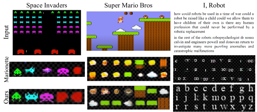
Figure 4: Ours on MarioNette and recovered concepts.

Table 1: Segmentation performance. Decomposition accuracy measured by the ARI metric. Second best values are underlined, while (^∗) uses the same element transformations and number of concepts as our method. See Section 6.1 for details.

	Tetrominoes	dSprites Color.	dSprites Bin.	dSprites Adv.	CLEVR6
IODINE	99.2 $\pm$ 0.4	76.7 $\pm$ 5.6	64.8 $\pm$ 17.2	-	98.8 $\pm$ 0.0
Slot Attention	99.5 $\pm$ 0.2	91.3 $\pm$ 0.3	69.4 $\pm$ 0.9	12.7 $\pm$ 1.1	98.8 $\pm$ 0.3
DTI-Sprites	99.6 $\pm$ 0.2	92.5 $\pm$ 0.3	$75.5^{*}\pm$ 0.4	$75.3^{*}\pm$ 0.4	97.2 $\pm$ 0.2
Ours	99.5 $\pm$ 0.1	$90.6\pm$ 0.8	85.1 $\pm$ 0.7	76.4 $\pm$ 2.4	64.6 $\pm$ 0.8

Figures 3 and S7 show example decompositions on each dataset. We provide the full dictionaries of visual concepts extracted from each dataset in the supplemental. DTI-Sprites is most related to our method. Table 1 shows our competitive segmentation performance, but Table S2 and Figure 6 reveal that the concepts it learns each may entangle multiple ground truth visual concepts, especially when using lower concept numbers. When reconstructing a scene, their image formation model needs to disentangle these concepts. Thus, it does often not correctly identify the concepts in a dataset.

In Fig 4 we should comparision between our method and Marionette, our method requires less data to extract concepts, only 4 and 6 frames for Space Invaders and Super Mario Bros, respectively, compared to several thousands of frames required by MarioNette.

Table 2: Visual concept error. Average $L_{1}$ distances between each library concept and the nearest learned concept.

	dSprites Bin	dSprites Adv
Slot Att.	0.0312	0.0497
DTI-Sprites	0.0133	0.0219
Ours	0.0033	0.0051

Table 3: Cross-dataset reconstruction. MSE reconstruction loss on EMNIST letters for methods trained on MNIST digits.

	MNIST(Train)	EMNIST(Test)
Slot Att.	0.0048	0.0560
DTI-Sprites	0.0065	0.0202
Ours(128)	0.0114	0.0169
Ours(512)	0.0090	0.0140

6.2 Cross-dataset Reconstruction

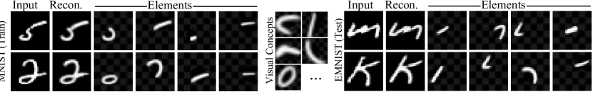
Figure 5: The visual concepts learned on one dataset (MNIST, left), can generalize to a second dataset (EMNIST, right), without further training.

To quantify generalization performance, we train our algorithm and the baselines on the MNIST [LeCun(1998)] dataset, which contains hand-written digits, and test their reconstruction performance on EMNIST [Cohen et al.(2017)Cohen, Afshar, Tapson, and Van Schaik] dataset, which also contains hand-written letters. Table 3 shows a quantitative comparison between Slot Attention, DTI-Sprites and two versions of our method using the MSE reconstruction loss, with the visual dictionary size capped to $128$ or $512$. Figure 5 shows an example decomposition. Since we do not rely on learned priors in addition to our dictionary, our inference pipeline shows significantly better generalization performance than the baselines. Note that in this experiment, DTI-Sprites is allowed translation, rotation and scaling of elements, while our method only uses translations.

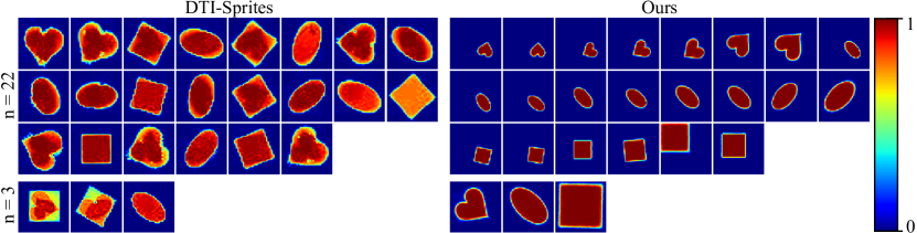
Figure 6: Comparison between visual concepts learned by DTI-Sprites and our method on the M-dSprites Bin. dataset with different dictionary sizes $n$. The heatmap shows pixel intensities. DTI-sprites learns entangled concepts that correspond to multiple ground truths.

Limitations.

Our pipeline has two main limitations. First, the computational cost of the element parameter search. We plan to optimize the search operation using techniques like a coarse-to-fine search in future work. Second, we currently search for exact repetitions of objects to learn our concepts. Accounting for deformations/variations by incorporating a more general parametric deformation model, for example by using a neural network with the help of differentiable rasterizers, will be a valuable next step towards a more general model.

7 Conclusion and Future Work

We presented a general method to learn visual concepts from data, both for images and shapes, without explicit supervision or learned priors. Our main idea is posing the search for visual concepts as a direct optimization, which can be solved efficiently when splitting the task into alternating dictionary finding and parameter optimization steps. Using direct optimization, instead of a network-based approach, improves the quality of the resulting visual concepts and additionally reveals parameters such as hue, position, and scale that are not available to most network-based approaches. In the future, we would like to extend our approach to a fully generative model. One approach would be to learn a distribution over the element parameters. When combined with the learned concepts, we could sample the element parameter distributions to produce new images with the given image formation function. This opens up new avenues for parametric generative models, blurring the line between neuro-symbolic and image-based generative models. We believe that ultimately the right direction for a decomposition is a hybrid between network-based and search-based methods.

S.1 Convolution-based Grid Search

When optimizing the element parameters in a given image $\tilde{I}$, we maximize the normalized cross-correlation [Kaso(2018)] instead of minimizing the $L_{2}$ distance:

$$\operatorname*{arg\,max}_{\theta_{1},\dots,\theta_{n}}\frac{\sum_{p}(I\tilde{I})_{p}}{\sqrt{\sum_{p}I^{2}_{p}}\hskip 5.0pt\sqrt{\sum_{p}\tilde{I}^{2}_{p}}}\quad\text{with }\tilde{I}=h(e_{\mathcal{V}}(\theta_{1}),\dots,e_{\mathcal{V}}(\theta_{n})),$$ (S1)

where the products are element-wise and p is a two-dimensional pixel index. We can then formulate a grid search over translation parameters as a convolution. In the single-element case, $\tilde{I}=E_{1}$, and we can rewrite Eq. S1 as:

$$\operatorname*{arg\,max}_{\theta_{1}}\frac{(I\circledast\hat{E}_{1})_{t_{1}}}{\sqrt{\sum_{p}I^{2}_{p}}\hskip 5.0pt\sqrt{(\mathbf{1}\circledast\hat{E}_{1}^{2})_{t_{1}}}},$$ (S2)

where $\hat{E}$ is the element $E$ with translation parameters $t\in\theta$ zeroed out, so the transformed visual concept is at the origin and acts as a convolution kernel, and $\mathbf{1}$ is an image of all-ones. The result of the convolution is an image where each pixel corresponds to the correlation at one 2D translation $t$.

In the general case with multiple elements, we optimize the parameters of one element at a time. At each element, we need to account for occlusions from previous elements when performing the convolution. Re-writing the alpha-composite defined in Eq. 1 to isolate the contribution of a single element $E_{i}$ we get:

$$\tilde{I}=\tilde{I}_{1}^{i-1}+E_{i}O_{1}^{i-1}+(1-E_{i}^{\text{A}})O_{1}^{i-1}\tilde{I}_{i+1}^{n}$$ (S3)

$$\text{with }\tilde{I}_{a}^{b}\coloneqq\sum_{i=a}^{b}E_{i}O_{a}^{i-1}\;\text{and }O_{a}^{j}\coloneqq\prod_{i=a}^{j}(1-E_{i}^{\text{A}}).$$

Intuitively, $\tilde{I}_{a}^{b}$ is the partial composite of the elements $a$ through $b$, without taking into account other elements, and $O_{a}^{j}$ is the occlusion effect of elements $a$ through $j$ on the following elements. Only the second and third terms depend on $L_{i}$, where the second term is the occluded contribution of $L_{i}$ to the image and the third term describes the occlusion caused by $L_{i}$ on the following elements. Substituting into Eq. S1, and using convolutions for searching over translations we arrive at:

$$\operatorname*{arg\,max}_{\theta_{i}}\frac{\sum_{p}(IC_{1})_{p}+(IC_{2}\circledast\hat{E}_{i}+IC_{3}\circledast(1-\hat{E}_{i}^{A}))_{t_{i}}}{\sqrt{\sum_{p}I^{2}_{p}}\hskip 5.0pt\sqrt{\sum_{p}(C_{1}^{2})_{p}+(\mathcal{N}_{i})_{t_{i}}}}$$ (S4)

$$\begin{aligned} \text{with }\mathcal{N}_{i}=\ &C_{2}^{2}\circledast\hat{E}_{i}^{2}+C_{3}^{2}\circledast(1-\hat{E}_{i}^{A})^{2}\\ &+2C_{1}C_{2}\circledast\hat{E}_{i}+2C_{1}C_{3}\circledast(1-\hat{E}_{i}^{A})\\ &+2C_{2}C_{3}\circledast\hat{E}_{i}(1-\hat{E}_{i}^{A})\end{aligned}$$

$$\text{and }C_{1}=\tilde{I}_{1}^{i-1}\hskip 10.0ptC_{2}=O_{1}^{i-1}\hskip 10.0ptC_{3}=O_{1}^{i-1}\tilde{I}_{i+1}^{n},$$

which we solve as efficient update step for element parameters. Section S.2 provides the derivation.

S.2 Layer Parameter Objective

We derive the objective for the layer parameter optimization with alpha compositing and convolutions defined in Eq. 7 of the main paper. The objective is obtained in two steps: (i) we substitute the alpha composite defined in Eq. 6 into layer parameter objective in Eq. 4, and (ii) we search over position parameters using convolutions, analogous to Eq. 5. For clarity, we first define:

$$C_{1}=\tilde{I}_{1}^{i-1}\hskip 10.0ptC_{2}=O_{1}^{i-1}\hskip 10.0ptC_{3}=O_{1}^{i-1}\tilde{I}_{i+1}^{n},$$

so that Eq. 6 becomes:

$$\tilde{I}=C_{1}+E_{i}C_{2}+(1-E_{i}^{\text{A}})C_{3}.$$ (S5)

Substituting Eq. S5 into Eq. 4 and restricting the optimization over the parameters $\theta_{i}$ of layer $E_{i}$:

$$\operatorname*{arg\,max}_{\theta_{i}}\frac{\sum_{p}(IC_{1})_{p}+\sum_{p}(IC_{2}E_{i})_{p}+\sum_{p}(IC_{3}(1-E_{i}^{A}))_{p}}{\sqrt{\sum_{p}I^{2}_{p}}\hskip 5.0pt\sqrt{\sum_{p}(C_{1}^{2})_{p}+\mathcal{N}^{\prime}_{i}}}$$ (S6)

$$\begin{aligned} \text{with }\mathcal{N}^{\prime}_{i}=\ &\textstyle\sum_{p}(C_{2}^{2}E_{i}^{2})_{p}\\ &+\textstyle\sum_{p}(C_{3}^{2}(1-E_{i}^{A})^{2})_{p}\\ &+2\textstyle\sum_{p}(C_{1}C_{2}E_{i})_{p}\\ &+2\textstyle\sum_{p}(C_{1}C_{3}(1-E_{i}^{A}))_{p}\\ &+2\textstyle\sum_{p}(C_{2}C_{3}E_{i}(1-E_{i}^{A}))_{p}.\end{aligned}$$

Finally, exchanging any term of the form $\sum_{p}(CE_{i})_{p}$ with a convolution $(C\circledast\hat{E}_{i})_{t_{i}}$ using as kernel the layer with with zeroed translation parameters $\hat{E}_{i}$, we arrive at Eq. 7 of the paper:

$$\operatorname*{arg\,max}_{\theta_{i}}\frac{\sum_{p}(IC_{1})_{p}+(IC_{2}\circledast\hat{E}_{i}+IC_{3}\circledast(1-\hat{E}_{i}^{A}))_{t_{i}}}{\sqrt{\sum_{p}I^{2}_{p}}\hskip 5.0pt\sqrt{\sum_{p}(C_{1}^{2})_{p}+(\mathcal{N}_{i})_{t_{i}}}}$$

$$\begin{aligned} \text{with }\mathcal{N}_{i}=\ &C_{2}^{2}\circledast\hat{E}_{i}^{2}\\ &+\sum C_{3}^{2}-2C_{3}^{2}\circledast\hat{E}_{i}^{A}+C_{3}^{2}\circledast(\hat{E}_{i}^{A})^{2}\\ &+2C_{1}C_{2}\circledast\hat{E}_{i}\\ &+2\sum C_{1}C_{3}-C_{1}C_{3}\circledast\hat{E}_{i}^{A}\\ &+2C_{2}C_{3}\circledast\hat{E}_{i}-2C_{2}C_{3}\circledast\hat{E}_{i}\hat{E}_{i}^{A}.\end{aligned}$$

S.3 Datasets and Hyperparameters details

The Tetrominoes dataset contains $60$k images with 3 randomly rotated and positioned Tetris blocks. The Multi-dSprites dataset consists of $60$k images, each showing 2-3 shapes picked from a dictionary and placed at random locations, possibly with occlusions. We use a discretized variant of the color version and the binarized version of this dataset. We discretize the color version to eight colors, so that the colors can be discovered as composite concepts. In addition, we create a variant of this dataset that we name Multi-dSprites adversarial, where shapes can only appear in three discrete locations on the canvas. This intuitively simple dataset highlights shortcomings in existing methods. The Clevr6 dataset consists of $35$k rendered 3D scenes with each scene is an arrangement of up to six geometric primitives with various colors and materials. Also since MarioNette data is not available, we obtain comparable data through screen captures of Space Invaders, Super Mario Bros, and I, Robot (in the latter we use only lower-case letters).

Optimization details.

We learn visual concepts using AdaDelta [Zeiler(2012)] with a learning-rate of $1.0$ and a batch size of $8$ on a single GPU. We have tested different optimizers but found that our pipeline was robust to the choice of optimizer. A more detailed comparison of optimizers is in the supplemental. We do not use any learning rate schedulers or warm-up techniques.

In Table S1 we list the hyperparameters we used for each experiment.

Table S1: Hyperparameters. In this table present the hyperparameters used of different experiments that are used to generate the results presented in the paper. Translation values are greater than the input image size if we allow partial placement of a concept. The first and second columns show the initial number of concepts and the max number of concepts . The rotation column indicates the number of values uniformly sampled in $[0,2\pi]$.

s Init Max Translation Rotation nColors nlayers Concept Size Tetris 1 10 35x35 4 6 3 19 Multi dSprites bin 4 22 64x64 40 1 3 33 Multi dSprites Adv 1 3 64x64 40 1 3 33 Clevr6 8 32 64x64 1 8 6 31 MNIST(128) 8 128 28x28 1 1 4 13 MNIST(512) 8 512 28x28 1 1 4 13 MNIST Sum(128) 8 128 41x41 1 1 4 13 MNIST Sum(512) 8 512 41x41 1 1 4 13 GTSRB 6 64 28x28 1 1 6 31 Xmas Pattern 2 2 85x85 1 1 45 21

S.4 Thresholds for Splitting and Removing Concepts

The threshold for removing a concept $V_{j}$ is $N_{j}<0.25\frac{n|\mathcal{I}|}{|\mathcal{V}|}$, where $N_{j}$ is the number of instances of concept $v_{j}$, and $n$ is the number of elements per image. The threshold for splitting a concept is $N_{j}>0.25\frac{n|\mathcal{I}|}{|\mathcal{V}|}$, in addition to a threshold on the reconstruction error $\mathcal{E}_{j}<0.95$. The reconstruction error $\mathcal{E}_{j}$ of a single visual concept $V_{j}$ over the whole dataset is isolated as:

$$\mathcal{E}_{j}(\mathcal{V},\Theta)\coloneqq\sum_{\{i,k|\tau^{k}_{i}=j\}}\frac{\sum_{p}(M^{k}_{i}I\tilde{I}M^{k}_{i})_{p}}{\sqrt{\sum_{p}(M^{k}_{i}I)_{p}^{2}}\sqrt{\sum_{p}(M^{k}_{i}\tilde{I})_{p}^{2}}}\quad\text{with }M^{k}_{i}=(E^{A}_{i})^{k}(O_{1}^{i-1})^{k}.$$ (S7)

The sum is over all elements $E^{k}_{i}$ in all images $I^{k}$ that use the visual concept $V_{j}$ and $M^{k}_{i}$ is a mask that zeros out parts of the image that do not have contributions from element $E^{k}_{i}$.

S.5 Concept Evolution Graph

As described in the main paper, the number of concepts is determined by a concept evolution approach where concepts can be split or removed. This results in a tree of visual concepts that is grown during optimization. An illustration of such a tree is shown in Figure S1.

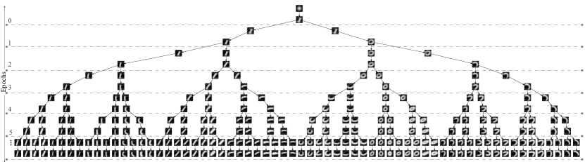
Figure S1: Visual concept evolution for the MNIST dataset. Note how the concepts evolve over optimization epochs by specializing to subtle stroke variations.

S.6 Learning Visual Concepts in 3D Scenes

We use our framework to learn 3D visual concepts $\mathcal{V}$ from multi-view renders of 3D scenes. In this setting, our visual concepts are 3D voxel patches instead of 2D image patches, where each voxel describes a density value. The transformation function $T$ translates these patches and samples them at the global voxel grid of the 3D scene to obtain 3D elements $E_{i}$: $E_{i}=T(V_{\tau_{i}},t_{i}),$ where $t_{i}$ is a 3D translation and $V_{\tau_{i}}$, a visual concept, is a 3D voxel patch containing density values. For the image formation function $h$, we use the orthographic projection to accumulate the voxel densities along the viewing direction $d$, giving us the image $\tilde{I}$:

$$\tilde{I}=h(E_{1},\dots,E_{n}|d)\coloneqq\sum_{l}\big{(}S^{2}_{jkl}\prod_{m=1}^{l-1}(1-S_{jkm})\big{)},\text{ with }S=\min(1,R_{d}\big{(}\sum_{i}{E_{i}}\big{)}),$$ (S8)

where $S$ is the scene voxel grid, computed as a sum over all element voxel grids, rotated and re-sampled by $R_{d}$ to align the last axis (indexed by $l$) with the viewing direction $d$. We clamp densities in $S$ to have a maximum of value $1$. The orthographic projection accumulates voxel densities along the viewing direction and the product attenuates voxel contributions by the occlusion effect of voxels closer to the viewer, indicated by smaller index $l$. We optimize element parameters $t_{i}$ and visual concepts $\mathcal{V}$ to maximize the normalized cross-correlation between all reconstructed renders $\tilde{I}$ and all ground truth renders $I$ of a 3D scene dataset, as described in the previous sections, but without using convolutions to speed up the search for element parameters. The element parameters $t_{i}$ of a scene are optimized using all views of that scene. In our experiments, we use $20$ views: back/front, left/right, top, and 3 additional rotations of these views by ${\pi}/{8}$ radians about the top/bottom axis.

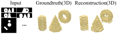
(a)

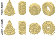
(b)

Figure S2: Given multi-view 2D renders of 3D scenes (left), our method can learn 3D visual concepts that can be used to reconstruct the 3D scenes.

Evaluation:

We create a synthetic dataset of $16$ 3D scenes by randomly selecting $3$ shapes from a dictionary of $4$ ground truth shapes and placing them at random positions on a ground plane. We render 20 different views of each scene to form the input dataset, and use the image formation described in Section S.6 to learn 3D concepts. Reconstruction results and a comparison of the learned concepts to the ground truth is provided in Figure S2.

S.7 Additive Compositing

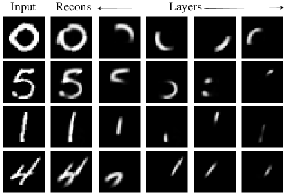
Figure S3: Example decomposition of an MNIST digit using additive compositing.

As mentioned in the main paper, we can use our approach with different compositing functions. Here, we present details and experiments with additive compositing instead of the alpha-compositing used for the 2D results in the main paper and the other sections of the supplementary. For additive compositing, we replace Eq. 6 with a sum over layers:

$$\tilde{I}=C+E_{i}$$ (S9)

$$\text{with }C=\sum_{j\neq i}E_{j}.$$

The layer parameter optimization objective defined by Eq. 7 for alpha composting then becomes the following for additive compositing:

$$\operatorname*{arg\,max}_{\theta_{i}}\frac{\sum_{p}(IC)_{p}+(I\circledast\hat{E}_{i})_{t_{i}}}{\sqrt{\sum_{p}I^{2}_{p}}\hskip 5.0pt\sqrt{\sum_{p}(C^{2})_{p}+(\mathbf{1}\circledast\hat{E}^{2}_{i})_{t_{i}}+(2C\circledast\hat{E}_{i})_{t_{i}}}}.$$ (S10)

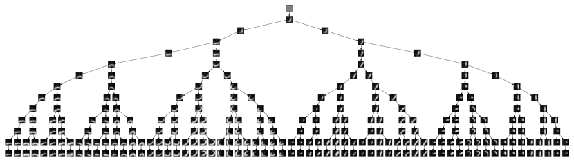
Figure S4: Graph illustrating visual concept evolution for the MNIST dataset trained using additive compositing. (Please use digital zoom for details.) Note how the method learns smaller concepts compared to alpha compositing, as shown in Figure 4 of the main paper.

Quantiative results measuring the MSE reconstruction loss for the cross-dataset generalization experiment are shown in Table S2 for two dictionary sizes. Note that reconstruction errors are slightly higher with additive compositing when compared to the corresponding results with alpha-compositing in Table 3 of the main paper. Figures S5 and S3 show the learned concepts and a decomposition example, respectively. Figure S4 show the evolution graph of the visual concepts.

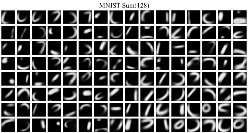
Figure S5: Visual concepts learned from the MNIST dataset using additive compositing.

Table S2: Additive compositing results. MSE reconstruction loss of EMNIST letters using additive compositing. The visual concepts are trained on the MNIST digits dataset with an additive compositing function. We show results for two dictionary sizes, $m=128$ and $m=512$.

	MNIST(Train)	EMNIST(Test)
Ours Additive (128)	0.0163	0.0215
Ours Additive (512)	0.0137	0.0186

S.8 Additional Results

We also submit an additional set of uncurated results along with the supplementary (see the contents of the zip file). We included the first $b$ images of the respective datasets, with $b$ being the batch-size. For each image, we show the reconstruction and the decomposed layers. Note that these results are not post-processed, so the layer decomposition may also contain layers that are completely occluded by other layers.

S.9 Comparison with Traditional methods

We compare our approach to traditional unsupervised decomposition methods like PCA or dictionary learning in Figure S6.

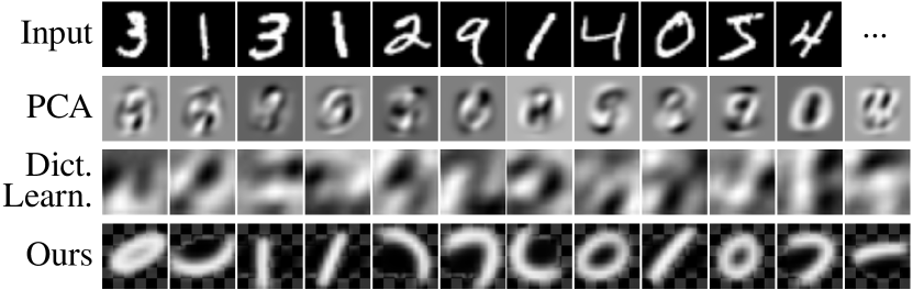
Figure S6: We show the performance of classical methods like PCA or dictionary learning to obtain dominant modes of an image dataset. Note that extracted modes are not very interpretable in terms of compositionality. In contrast, our method uses a search-and-learn strategy to extract a dictionary of interpretable visual concepts, in this case the underlying strokes. Checkered patterns denote transparent pixels.

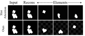
(a)

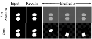
(b)

Figure S7: Comparison of decomposition result to Slot Attention on the M-dSprites Bin. and M-dSprites Adv. datasets. Slot Attention is not regularized by a global dictionary, resulting in incorrect decompositions. Ours are more interpretable.

S.10 Ablation of Optimizers

We demonstrate the robustness of our approach to the choice of optimizer and learning rates. In Figure S8, we show the MSE training loss curve for different optimizers and learning rates on the pattern images shared along with this supplementary material. We show SGD, Adam [Kingma and Ba(2014)], Adadelta [Zeiler(2012)], and RMSprop optimizers with learning rates in $[0.001,1]$. Our pipeline converges for all the optimizers with appropriate learning rate but lower learning rates take longer to converge.

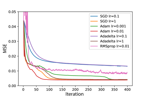
Figure S8: MSE training loss curves for various optimizers and learning rates. Note that all optimizers converge with the right learning rate.

S.11 Ablation of the Visual Concept Evolution

In Fig S9, we demonstrate the necessity for the visual concept evolution in our pipeline. Without evolution, a single optimized concept may average multiple similar ground truth concepts. Using evolution, we allow this average concept to split into multiple more specialized child-concepts, that each approximate fewer ground truth concepts. After a few evolution steps, each leaf concept eventually represents a single ground truth concept.

(a)

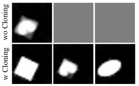
(b)

Figure S9: Effect of cloning. Without cloning (left-top) our algorithm produces an average visual concept as a proxy to collectively represent similar shapes. However, with cloning (left-bottom) our algorithm can specialize to pickup subtle differences among the visual concepts, producing individualized concepts. On the right, we show the confusion matrix to show how similar the ground truth visual concepts are, with $1$ denoting perfect similarity.

S.12 ARI calculation

The Adjusted Rand Index (ARI) measures the similarity between two clusterings. We use it to compare the decomposition found by our method to the ground truth decomposition. In images without occlusions or with visual concepts that have the same constant color, any layer ordering results in the same reconstructed image, thus the layer order is ambiguous. In cases with ambiguous ordering, we select the layer ordering that gives the highest ARI score.

S.13 Full visual concepts

In Figures S10 and S11, we show all visual concepts learned by our method from each 2D dataset used in the main paper (all visual concepts of the 3D dataset are shown in Figure 10 of the main paper). Additionally, we show visual concepts obtained from the GTSRB traffic sign dataset [Stallkamp et al.(2012)Stallkamp, Schlipsing, Salmen, and Igel] in Figure S11, bottom.

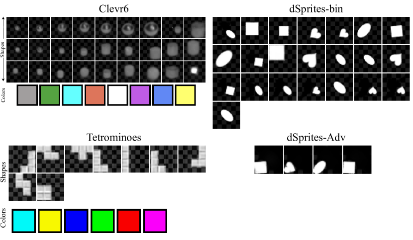
Figure S10: All the learned concepts on Tetrominoes, Multi-dSprites bin, Multi-dSprites Adv and Clevr6 datasets.

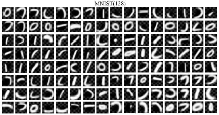
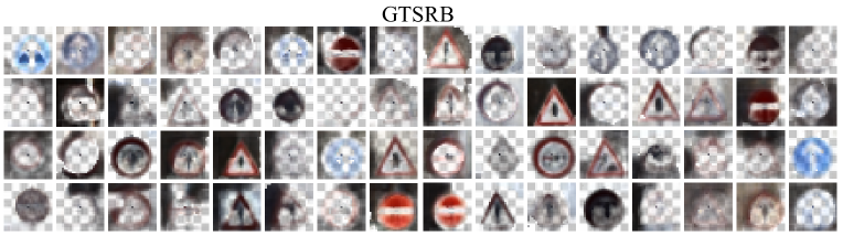
Figure S11: All the learned concepts on MNIST and GTSRB datasets.

S.14 dSprites Adv. Dataset Details

To create the dSprites Adversarial dataset, we place two or three visual concepts in each image. Each concept is placed at one of three pre-defined locations on the canvas (without overlaps). All concepts have the same scale and a random rotation. Figure S12 shows samples of the dataset.

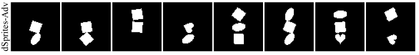
Figure S12: Random samples from the dSprites Adversarial Dataset.

S.15 Background Handling

When using alpha-compositing, we treat the background as a special layer $L_{n}$ that is locked to the back of the layer stack (i.e. it is occluded by all other layers when using alpha-compositing) and does not have layer parameters. The background is represented by a special visual concept $V_{m}$ that is only used by the background layer and is initialized with a constant value of $0.5$ in all pixels. During optimization of a given image $\tilde{I}$, we optimize the background visual concept before the other concepts or layers, to make sure the other layers don’t represent parts of the background.

S.16 3D Scene Reconstruction segmentation

We also measure the quality of our decompositions by comparing the 2D projections of the segmented 3D scene to a known ground truth. We achieve an ARI of 99.3% on this task.

S.17 Video

In the supplementary material, we include a video that visualizes the optimization process of our method, showing the optimized visual concepts in each iteration and the layer segmentation of the reconstructed image. For clarity, we demonstrate the optimization on a dataset consisting of a single image with multiple repeating visual concepts.

S.18 Code

We include a development version of our code in the supplemental that can be used to reproduce the results.

References

- [Badrinarayanan et al.(2015)Badrinarayanan, Handa, and Cipolla] Vijay Badrinarayanan, Ankur Handa, and Roberto Cipolla. Segnet: A deep convolutional encoder-decoder architecture for robust semantic pixel-wise labelling. arXiv preprint arXiv:1505.07293, 2015.
- [Burgess et al.(2019)Burgess, Matthey, Watters, Kabra, Higgins, Botvinick, and Lerchner] Christopher P Burgess, Loic Matthey, Nicholas Watters, Rishabh Kabra, Irina Higgins, Matt Botvinick, and Alexander Lerchner. Monet: Unsupervised scene decomposition and representation. arXiv preprint arXiv:1901.11390, 2019.
- [Carion et al.(2020)Carion, Massa, Synnaeve, Usunier, Kirillov, and Zagoruyko] Nicolas Carion, Francisco Massa, Gabriel Synnaeve, Nicolas Usunier, Alexander Kirillov, and Sergey Zagoruyko. End-to-end object detection with transformers. In European Conference on Computer Vision, pages 213–229. Springer, 2020.
- [Chen et al.(2017)Chen, Papandreou, Kokkinos, Murphy, and Yuille] Liang-Chieh Chen, George Papandreou, Iasonas Kokkinos, Kevin Murphy, and Alan L Yuille. Deeplab: Semantic image segmentation with deep convolutional nets, atrous convolution, and fully connected crfs. IEEE transactions on pattern analysis and machine intelligence, 40(4):834–848, 2017.
- [Chen et al.(2019)Chen, Varma, Krishna, Bernstein, Re, and Fei-Fei] Vincent S Chen, Paroma Varma, Ranjay Krishna, Michael Bernstein, Christopher Re, and Li Fei-Fei. Scene graph prediction with limited labels. In Proceedings of the IEEE/CVF International Conference on Computer Vision, pages 2580–2590, 2019.
- [Chen et al.(2007)Chen, Zhu, Lin, Zhang, and Yuille] Yuanhao Chen, Long Zhu, Chenxi Lin, Hongjiang Zhang, and Alan L Yuille. Rapid inference on a novel and/or graph for object detection, segmentation and parsing. Advances in neural information processing systems, 20:289–296, 2007.
- [Cohen et al.(2017)Cohen, Afshar, Tapson, and Van Schaik] Gregory Cohen, Saeed Afshar, Jonathan Tapson, and Andre Van Schaik. Emnist: Extending mnist to handwritten letters. In 2017 International Joint Conference on Neural Networks (IJCNN), pages 2921–2926. IEEE, 2017.
- [Ehrhardt et al.(2020)Ehrhardt, Groth, Monszpart, Engelcke, Posner, J. Mitra, and Vedaldi] Sébastien Ehrhardt, Oliver Groth, Aron Monszpart, Martin Engelcke, Ingmar Posner, Niloy J. Mitra, and Andrea Vedaldi. RELATE: Physically plausible multi-object scene synthesis using structured latent spaces. NeurIPS, 2020.
- [Engelcke et al.(2019)Engelcke, Kosiorek, Jones, and Posner] Martin Engelcke, Adam R Kosiorek, Oiwi Parker Jones, and Ingmar Posner. Genesis: Generative scene inference and sampling with object-centric latent representations. arXiv preprint arXiv:1907.13052, 2019.
- [Engelcke et al.(2021)Engelcke, Jones, and Posner] Martin Engelcke, Oiwi Parker Jones, and Ingmar Posner. Genesis-v2: Inferring unordered object representations without iterative refinement. arXiv preprint arXiv:2104.09958, 2021.
- [Girshick(2015)] RJCS Girshick. Fast r-cnn. arxiv 2015. arXiv preprint arXiv:1504.08083, 2015.
- [Girshick et al.(2014)Girshick, Donahue, Darrell, and Malik] Ross Girshick, Jeff Donahue, Trevor Darrell, and Jitendra Malik. Rich feature hierarchies for accurate object detection and semantic segmentation. In Proceedings of the IEEE conference on computer vision and pattern recognition, pages 580–587, 2014.
- [Goyal et al.(2019)Goyal, Lamb, Hoffmann, Sodhani, Levine, Bengio, and Schölkopf] Anirudh Goyal, Alex Lamb, Jordan Hoffmann, Shagun Sodhani, Sergey Levine, Yoshua Bengio, and Bernhard Schölkopf. Recurrent independent mechanisms. arXiv preprint arXiv:1909.10893, 2019.
- [Greff et al.(2017)Greff, Van Steenkiste, and Schmidhuber] Klaus Greff, Sjoerd Van Steenkiste, and Jürgen Schmidhuber. Neural expectation maximization. arXiv preprint arXiv:1708.03498, 2017.
- [Greff et al.(2019)Greff, Kaufman, Kabra, Watters, Burgess, Zoran, Matthey, Botvinick, and Lerchner] Klaus Greff, Raphaël Lopez Kaufman, Rishabh Kabra, Nick Watters, Christopher Burgess, Daniel Zoran, Loic Matthey, Matthew Botvinick, and Alexander Lerchner. Multi-object representation learning with iterative variational inference. In International Conference on Machine Learning, pages 2424–2433. PMLR, 2019.
- [Greff et al.(2020)Greff, van Steenkiste, and Schmidhuber] Klaus Greff, Sjoerd van Steenkiste, and Jürgen Schmidhuber. On the binding problem in artificial neural networks. arXiv preprint arXiv:2012.05208, 2020.
- [He et al.(2017)He, Gkioxari, Dollár, and Girshick] Kaiming He, Georgia Gkioxari, Piotr Dollár, and Ross Girshick. Mask r-cnn. In Proceedings of the IEEE international conference on computer vision, pages 2961–2969, 2017.
- [Hinton et al.(2018)Hinton, Sabour, and Frosst] Geoffrey E Hinton, Sara Sabour, and Nicholas Frosst. Matrix capsules with em routing. In International conference on learning representations, 2018.
- [Johnson et al.(2017)Johnson, Hariharan, Van Der Maaten, Fei-Fei, Lawrence Zitnick, and Girshick] Justin Johnson, Bharath Hariharan, Laurens Van Der Maaten, Li Fei-Fei, C Lawrence Zitnick, and Ross Girshick. Clevr: A diagnostic dataset for compositional language and elementary visual reasoning. In Proceedings of the IEEE conference on computer vision and pattern recognition, pages 2901–2910, 2017.
- [Jojic et al.(2003)Jojic, Frey, and Kannan] Nebojsa Jojic, Brendan J Frey, and Anitha Kannan. Epitomic analysis of appearance and shape. In Computer Vision, IEEE International Conference on, volume 2, pages 34–34. IEEE Computer Society, 2003.
- [Kaso(2018)] Artan Kaso. Computation of the normalized cross-correlation by fast fourier transform. PLOS ONE, 13(9):1–16, 09 2018. 10.1371/journal.pone.0203434. URL https://doi.org/10.1371/journal.pone.0203434.
- [Kingma and Ba(2014)] Diederik P Kingma and Jimmy Ba. Adam: A method for stochastic optimization. arXiv preprint arXiv:1412.6980, 2014.
- [Kosiorek et al.(2019)Kosiorek, Sabour, Teh, and Hinton] Adam R Kosiorek, Sara Sabour, Yee Whye Teh, and Geoffrey E Hinton. Stacked capsule autoencoders. arXiv preprint arXiv:1906.06818, 2019.
- [Kosiorek et al.(2020)Kosiorek, Kim, and Rezende] Adam R Kosiorek, Hyunjik Kim, and Danilo J Rezende. Conditional set generation with transformers. arXiv preprint arXiv:2006.16841, 2020.
- [Krishna et al.(2016)Krishna, Zhu, Groth, Johnson, Hata, Kravitz, Chen, Kalantidis, Li, Shamma, et al.] Ranjay Krishna, Yuke Zhu, Oliver Groth, Justin Johnson, Kenji Hata, Joshua Kravitz, Stephanie Chen, Yannis Kalantidis, Li-Jia Li, David A Shamma, et al. Visual genome: Connecting language and vision using crowdsourced dense image annotations. arXiv preprint arXiv:1602.07332, 2016.
- [LeCun(1998)] Yann LeCun. The mnist database of handwritten digits. http://yann. lecun. com/exdb/mnist/, 1998.
- [Lee et al.(2019)Lee, Lee, Kim, Kosiorek, Choi, and Teh] Juho Lee, Yoonho Lee, Jungtaek Kim, Adam Kosiorek, Seungjin Choi, and Yee Whye Teh. Set transformer: A framework for attention-based permutation-invariant neural networks. In International Conference on Machine Learning, pages 3744–3753. PMLR, 2019.
- [Locatello et al.(2020)Locatello, Weissenborn, Unterthiner, Mahendran, Heigold, Uszkoreit, Dosovitskiy, and Kipf] Francesco Locatello, Dirk Weissenborn, Thomas Unterthiner, Aravindh Mahendran, Georg Heigold, Jakob Uszkoreit, Alexey Dosovitskiy, and Thomas Kipf. Object-centric learning with slot attention. arXiv preprint arXiv:2006.15055, 2020.
- [Lu et al.(2016)Lu, Krishna, Bernstein, and Fei-Fei] Cewu Lu, Ranjay Krishna, Michael Bernstein, and Li Fei-Fei. Visual relationship detection with language priors. In European conference on computer vision, pages 852–869. Springer, 2016.
- [Matthey et al.(2017)Matthey, Higgins, Hassabis, and Lerchner] Loic Matthey, Irina Higgins, Demis Hassabis, and Alexander Lerchner. dsprites: Disentanglement testing sprites dataset. https://github.com/deepmind/dsprites-dataset/, 2017.
- [Monnier et al.(2021)Monnier, Vincent, Ponce, and Aubry] Tom Monnier, Elliot Vincent, Jean Ponce, and Mathieu Aubry. Unsupervised layered image decomposition into object prototypes. arXiv preprint arXiv:2104.14575, 2021.
- [Nguyen-Phuoc et al.(2019)Nguyen-Phuoc, Li, Theis, Richardt, and Yang] Thu Nguyen-Phuoc, Chuan Li, Lucas Theis, Christian Richardt, and Yong-Liang Yang. Hologan: Unsupervised learning of 3d representations from natural images. In Proceedings of the IEEE/CVF International Conference on Computer Vision, pages 7588–7597, 2019.
- [Nguyen-Phuoc et al.(2020)Nguyen-Phuoc, Richardt, Mai, Yang, and Mitra] Thu Nguyen-Phuoc, Christian Richardt, Long Mai, Yong-Liang Yang, and Niloy Mitra. Blockgan: Learning 3d object-aware scene representations from unlabelled images. arXiv preprint arXiv:2002.08988, 2020.
- [Niemeyer and Geiger(2021)] Michael Niemeyer and Andreas Geiger. Giraffe: Representing scenes as compositional generative neural feature fields. In Proc. IEEE Conf. on Computer Vision and Pattern Recognition (CVPR), 2021.
- [Reddy et al.(2020)Reddy, Guerrero, Fisher, Li, and Mitra] Pradyumna Reddy, Paul Guerrero, Matt Fisher, Wilmot Li, and Niloy J Mitra. Discovering pattern structure using differentiable compositing. ACM Transactions on Graphics (TOG), 39(6):1–15, 2020.
- [Redmon et al.(2015)Redmon, Divvala, Girshick, and Farhadi] J Redmon, S Divvala, R Girshick, and A Farhadi. You only look once: Unified, real-time object detection. arxiv 2015. arXiv preprint arXiv:1506.02640, 2015.
- [Ren et al.(2015)Ren, He, Girshick, and Sun] Shaoqing Ren, Kaiming He, Ross Girshick, and Jian Sun. Faster r-cnn: Towards real-time object detection with region proposal networks. Advances in neural information processing systems, 28:91–99, 2015.
- [Sabour et al.(2017)Sabour, Frosst, and Hinton] Sara Sabour, Nicholas Frosst, and Geoffrey E Hinton. Dynamic routing between capsules. arXiv preprint arXiv:1710.09829, 2017.
- [Sitzmann et al.(2020)Sitzmann, Martel, Bergman, Lindell, and Wetzstein] Vincent Sitzmann, Julien N.P. Martel, Alexander W. Bergman, David B. Lindell, and Gordon Wetzstein. Implicit neural representations with periodic activation functions. In Proc. NeurIPS, 2020.
- [Smirnov et al.(2021)Smirnov, Gharbi, Fisher, Guizilini, Efros, and Solomon] Dmitriy Smirnov, Michael Gharbi, Matthew Fisher, Vitor Guizilini, Alexei A. Efros, and Justin Solomon. MarioNette: Self-supervised sprite learning. Conference on Neural Information Processing Systems, 2021.
- [Stallkamp et al.(2012)Stallkamp, Schlipsing, Salmen, and Igel] Johannes Stallkamp, Marc Schlipsing, Jan Salmen, and Christian Igel. Man vs. computer: Benchmarking machine learning algorithms for traffic sign recognition. Neural networks, 32:323–332, 2012.
- [Stelzner et al.(2021)Stelzner, Kersting, and Kosiorek] Karl Stelzner, Kristian Kersting, and Adam R Kosiorek. Decomposing 3d scenes into objects via unsupervised volume segmentation. arXiv preprint arXiv:2104.01148, 2021.
- [van Steenkiste et al.(2020)van Steenkiste, Kurach, Schmidhuber, and Gelly] Sjoerd van Steenkiste, Karol Kurach, Jürgen Schmidhuber, and Sylvain Gelly. Investigating object compositionality in generative adversarial networks. Neural Networks, 130:309–325, 2020.
- [Vinh et al.(2010)Vinh, Epps, and Bailey] Nguyen Xuan Vinh, Julien Epps, and James Bailey. Information theoretic measures for clusterings comparison: Variants, properties, normalization and correction for chance. The Journal of Machine Learning Research, 11:2837–2854, 2010.
- [Zeiler(2012)] Matthew D Zeiler. Adadelta: an adaptive learning rate method. arXiv preprint arXiv:1212.5701, 2012.
- [Zhang et al.(2019)Zhang, Hare, and Prugel-Bennett] Yan Zhang, Jonathon Hare, and Adam Prugel-Bennett. Deep set prediction networks. Advances in Neural Information Processing Systems, 32:3212–3222, 2019.
- [Zhao et al.(2017)Zhao, Shi, Qi, Wang, and Jia] Hengshuang Zhao, Jianping Shi, Xiaojuan Qi, Xiaogang Wang, and Jiaya Jia. Pyramid scene parsing network. In Proceedings of the IEEE conference on computer vision and pattern recognition, pages 2881–2890, 2017.
- [Zhu et al.(2010)Zhu, Chen, Torralba, Freeman, and Yuille] Long Zhu, Yuanhao Chen, Antonio Torralba, William Freeman, and Alan Yuille. Part and appearance sharing: Recursive compositional models for multi-view. In 2010 IEEE Computer Society Conference on Computer Vision and Pattern Recognition, pages 1919–1926. IEEE, 2010.
- [Zhu et al.(2008)Zhu, Lin, Huang, Chen, and Yuille] Long Leo Zhu, Chenxi Lin, Haoda Huang, Yuanhao Chen, and Alan Yuille. Unsupervised structure learning: Hierarchical recursive composition, suspicious coincidence and competitive exclusion. In European Conference on Computer Vision, pages 759–773. Springer, 2008.
- [Zhu and Mumford(2007)] Song-Chun Zhu and David Mumford. A stochastic grammar of images. Now Publishers Inc, 2007.