Spherical collapse of non-top-hat profiles in the presence of dark energy with arbitrary sound speed

Abstract

We study the spherical collapse of non-top-hat matter fluctuations in the presence of dark energy with arbitrary sound speed. The model is described by a system of partial differential equations solved using a pseudo-spectral method with collocation points. This method can reproduce the known analytical solutions in the linear regime with an accuracy better than $10^{-6}\%$ and better than $10^{-2}\%$ for the virialization threshold given by the usual spherical collapse model. We show the impact of nonlinear dark energy fluctuations on matter profiles, matter peculiar velocity and gravitational potential. We also show that phantom dark energy models with low sound speed can develop a pathological behaviour around matter halos, namely negative energy density. The dependence of the virialization threshold density for collapse on the dark energy sound speed is also computed, confirming and extending previous results in the limit for homogeneous and clustering dark energy.

1 Introduction

The Spherical Collapse (SC) model, as proposed by Gunn and Gott [1], describes the nonlinear evolution of pressureless matter perturbations in Einstein-de-Sitter Universe (EdS). This model can be used to determine the critical density of collapse, $\delta_{c}$, which can be used in Press-Schechter or Sheth-Tormen [2, 3] halo mass functions to compute the abundance of Dark Matter (DM) halos in the universe. However, the expansion of the universe is accelerating, which indicates that, assuming General Relativity correctly describes gravitational interactions on large scales, the universe is composed of roughly $70\%$ Dark Energy (DE) and $30\%$ of matter (DM plus barions) today. Even before the discovery of the accelerated expasion, the SC model has been generalized to include the Cosmological Constant, $\Lambda$, [4, 5, 6, 7]. Later, homogeneous DE models described as a perfect fluid were studied, e.g., [7, 8, 9, 10]. In these scenarios, DE induces a small (at most $1\%$) decay of $\delta_{c}$ at low-$z$ in comparison to the standard EdS value ($\delta_{c}\simeq 1.686$).

Recently, observational data has indicated that the value of the Hubble constant predicted by the $\Lambda$CDM model is in tension with local astrophysical measurements. There also exists a less significant tension related to the normalization of matter perturbations, expressed in terms of the $S_{8}=\sigma_{8}\left(\Omega_{m}^{0}/0.3\right)^{1/2}$ parameter. See [11] for a discussion and several proposals to solve these issues. If the accelerated expansion is not caused by $\Lambda$, DE necessarily has fluctuations, which might be important for the evolution of matter fluctuations on small scales, for a review, see [12]. For a concrete recent study of how DE perturbations can alleviate these tensions, see [13].

Several papers have studied the SC model and halo abundances in the presence of DE fluctuations, e.g., [14, 15, 16, 17, 18, 19, 20, 21, 22, 23, 24, 25, 26]. The key parameter that determines the impact of DE fluctuations is the sound speed $c_{s}=\sqrt{\delta p_{de}/\delta\rho_{de}}$. If $c_{s}\simeq 1$, DE fluctuations are much smaller than matter fluctuations on small scales and essentially do not modify the growth of nonlinear structures. The nonlinear evolution of Quintessence and Tachyon models were studied in [27]. For Quintessence, $c_{s}=1$, and its perturbation remains very small even when matter perturbations become nonlinear. As we will show, this also happens in the fluid description implemented in this work. In Tachyon models, $c_{s}^{2}=-w$ and, since $w\simeq-1$ at late times, the sound speed is also near the unity, erasing DE fluctuations on small scales.

On the order hand, if $c_{s}$ is sufficiently small, DE perturbation can be of the same magnitude as matter fluctuations. If $c_{s}\thickapprox 0$, DE fluctuations are effectively pressureless and behave as matter fluctuations. In this case, one can modify the SC model to include this extra clustering component [16, 18, 28]. However, for non-negligible $c_{s}$, DE fluctuations are affected by their pressure gradients, and do not follow the matter evolution. Therefore, the SC model has to be modified to account for this effect. The first effort in this direction was made in [20], which included DE linear perturbations in the evolution of the SC model.

Only in the last couple years, studies based on numerical N-body simulations codes began to include DE fluctuations. In [29], DE linear perturbations are included as a source of the gravitational potential. It was found that, even without nonlinear DE fluctuations, the matter power spectrum can change at the percent level. In [30], DE nonlinear fluctuations where treated, showing that they can indeed become nonlinear and change the formation of halos for $c_{s}^{2}=10^{-7}$. However, so far, this kind of studies did not yet consider the impact of $c_{s}$ on halo mass functions. As we will show, in terms of virialization threshold ($\delta_{{\rm v}}$) and density profiles, DE fluctuations become effectively pressureless for $c_{s}^{2}<10^{-5}$ on small nonlinear scales, but higher values also produce relevant changes with respect to the nearly homogeneous case with $c_{s}^{2}=1$.

In order to show these effects, we develop a method to solve the nonlinear evolution of perfect fluids with spherical symmetry, particularly in the case of pressureless matter and DE with arbitrary $w$ and $c_{s}$. We present the equations in the Pseudo-Newtonian framework and solve them numerically using the pseudo-spectral method with collocation points. We show the impact of $c_{s}$ on the linear and nonlinear evolution of matter fluctuations, matter peculiar velocities and gravitational potential. We also compute the threshold of virialization for various values of $c_{s}$, which can be used to estimate the impact of DE fluctuations on the abundance of halos.

Although this approach is not as realistic as a N-body simulation, it is much more economical in computational power, allowing us to understand the dependence of DE fluctuation on $c_{s}$, and not only for very low values. A typical code run takes about 10 minutes in an Intel i7 core, with very small memory use. The method can be easily generalized for other models, like coupled DE-DM, warm DM, modified gravity and Ultra Light DM. Therefore, we can easily explore model parameters and predict which scenario is potentially observationally distinguishable in view of current or future observations. This kind of study can also be a guide to more realistic simulations.

This paper is organized as follows. In section 2, we show the system of equations that describe the fluctuations in the two fluids and their initial conditions. In section 3, we present the numerical method used to solve the resulting equations. In section 4, we show the impact of $c_{s}$ on DM and DE profiles and discuss a pathology associated with the nonlinear evolution of phantom models ($w<-1$). We calculate the virialization threshold in section 5 and conclude in section 6.

2 Equations of motion

We will use the Pseudo-Newtonian Cosmology [31] in order to describe the evolution of pressureless matter and DE fluctuations in the nonlinear regime, written in physical coordinates. For each fluid, we have the following equations:

$$\frac{\partial\rho}{\partial t}+\vec{\nabla}\cdot\left(\vec{u}\rho\right)+p\vec{\nabla}\cdot\vec{u}=0\,,$$ (2.1)

$$\frac{\partial\vec{u}}{\partial t}+\left(\vec{u}\cdot\vec{\nabla}\right)\vec{u}=-\vec{\nabla}\Phi-\frac{\vec{\nabla}p}{\rho+p}\,,$$ (2.2)

and for the gravitational potential we have

$$\nabla^{2}\Phi=4\pi G\sum_{j}\left(\rho_{j}+3p_{j}\right)\,.$$ (2.3)

As usual, we split background and fluctuations quantities. Assuming spherical symmetry, all quantities depend on time and the radial coordinate, $r$, which we define as comoving with the background expansion:

$$\rho=\bar{\rho}\left(t\right)+\delta\rho\left(t,r\right)\,,$$ (2.4)

$$p=\bar{p}\left(t\right)+\delta p\left(t,r\right)\,,$$ (2.5)

$$\vec{u}=\vec{u}_{0}+v\left(t,r\right)\hat{r}\,,$$ (2.6)

$$\Phi=\Phi_{0}+\phi\left(t,r\right)\,.$$ (2.7)

We also assume a time-dependent equation of state for the background pressure,

$$\bar{p}_{de}=w\left(t\right)\bar{\rho}_{de}\,,$$ (2.8)

and a time-dependent sound speed, which relates the pressure and to density fluctuations

$$\delta p_{de}=c_{s}^{2}\left(t\right)\delta\rho_{de}\,.$$ (2.9)

Under these assumptions, the equations for the nonlinear evolution of pressureless matter and DE are given by:

$$\dot{\delta}_{m}+\left(1+\delta_{m}\right)\frac{\partial_{r}\left(r^{2}v_{m}\right)}{ar^{2}}+\frac{v_{m}\partial_{r}\delta_{m}}{a}=0\,,$$ (2.10)

$$\dot{v}_{m}+Hv_{m}+\frac{v_{m}\partial_{r}v_{m}}{a}=-\frac{\partial_{r}\phi}{a}\,,$$ (2.11)

$$\dot{\delta}_{de}+3H\left(c_{s}^{2}-w\right)\delta_{de}+\left[1+w+\left(1+c_{s}^{2}\right)\delta_{de}\right]\frac{\partial_{r}\left(r^{2}v_{de}\right)}{ar^{2}}+\frac{v_{de}\partial_{r}\delta_{de}}{a}=0\,,$$ (2.12)

$$\dot{v}_{de}+Hv_{de}+\frac{v_{de}\partial_{r}v_{de}}{a}=-\frac{\partial_{r}\phi}{a}-\frac{c_{s}^{2}\partial_{r}\delta_{de}}{a\left[1+w+\left(1+c_{s}^{2}\right)\delta_{de}\right]}\,,$$ (2.13)

$$\left(\partial_{r}^{2}+\frac{2}{r}\partial_{r}\right)\phi=\frac{3a^{2}H^{2}}{2}\left[\Omega_{m}\delta_{m}+\Omega_{de}\left(1+3c_{s}^{2}\right)\delta_{de}\right]\,.$$ (2.14)

For scales well above the sound horizon of DE, the term $c_{s}^{2}\partial_{r}\delta_{de}$ can be neglected, and equations (2.13) and (2.11) are identical, showing that both fluids flow in the same way. Under this assumption, clustering DE models have been studied in various scenarios [15, 32, 16, 33, 18, 21, 22, 23, 24]. The same problem was also studied for non-negligible sound speed, but assuming that dark energy perturbations are linear [20]. The main achievement of our work is the development of a numerical code capable of consistently solving the evolution of this type of model for arbitrary values of sound speed.

In the following, we assume a background evolution with flat spatial section, pressureless matter (baryons plus dark matter) and DE with CPL equation of state [34, 35] $w=w_{a}+\left(1-a\right)w_{a}$. Thus, the Hubble function is given by:

$$H^{2}=H_{0}^{2}\left(\Omega_{m}^{0}a^{-3}+\left(1-\Omega_{m}^{0}\right)f\left(a\right)\right),$$ (2.15)

where $f\left(a\right)=a^{-3\left(1+w_{0}+w_{a}\right)}\exp\left[3w_{a}\left(a-1\right)\right]$. In all examples shown, we assume $\Omega_{m}^{0}=0.3$. For simplicity, we also assume a constant $c_{s}$.

Initial conditions

We set the initial conditions in the matter-dominated era ($z_{i}=99$), making use of well-known analytical solutions in the linear regime, for instance, see [36, 37]. We assume an initial Gaussian profile for matter, which initially follows the EdS solution

$$\delta_{m}\left(a,r\right)=A\left(\frac{a}{a_{i}}\right)\exp\left(-\frac{r^{2}}{2\sigma^{2}}\right)\,.$$ (2.16)

Then we determine the initial velocity profile for matter with the linearized version of Eq. (2.10):

$$v_{m}\left(a_{i},r\right)=-\frac{a_{i}H_{i}}{r^{2}}\int_{0}^{r}dr^{\prime}\left(r^{\prime}\right)^{2}\delta_{m}\left(a_{i},r^{\prime}\right)\,.$$ (2.17)

The initial potential profile is determined assuming that, initially $\Omega_{m}\delta_{m}\gg\Omega_{de}\delta_{de}$:

$$\left(\partial_{r}^{2}+\frac{2}{r}\partial_{r}\right)\phi=\frac{3H_{i}^{2}}{2}\Omega_{m}\left(a_{i}\right)\delta_{m}\left(a_{i},r\right)\,,$$ (2.18)

which has the analytical solution

$$\phi=-\frac{3H_{i}^{2}}{2}\Omega_{m}\left(a_{i}\right)A\sigma^{3}\sqrt{\frac{\pi}{2}}\frac{1}{r}\text{erf}\left(\frac{r}{\sqrt{2}\sigma}\right)\,.$$ (2.19)

For DE, we implement two kinds of initial conditions, depending on the value of $c_{s}$. If $c_{s}<c_{sd}$, where $c_{sd}$ is some reference value below which DE fluctuations behave as dust, we have

$$\delta_{de}\left(a_{i},r\right)=\frac{1+w}{1-3w}\delta_{m}\left(a_{i},r\right)$$ (2.20)

and

$$v_{de}\left(a_{i},r\right)=v_{m}\left(a_{i},r\right)\,.$$ (2.21)

For $c_{s}>c_{sd}$, DE perturbations are much smaller then matter perturbations and the initial conditions are given by

$$\delta_{de}=-\frac{1+w}{c_{s}^{2}}\phi$$ (2.22)

and

$$v_{de}\left(a_{i},r\right)=-\frac{3a_{i}H_{i}\left(c_{s}^{2}-w\right)}{\left(1+w\right)r^{2}}\int_{0}^{r}dr^{\prime}\left(r^{\prime}\right)^{2}\delta_{de}\left(a_{i},r^{\prime}\right)\,.$$ (2.23)

Off course, in the case $c_{s}\sim c_{d}$ these initial conditions might not be quite satisfactory, but this is not an issue for the late-time evolution, when transient behavior due to imprecise initial conditions are usually negligible. As will be shown, for the small nonlinear scales, DE models with $c_{s}^{2}<10^{-3}$ begin to deviate significantly from the homogeneous case ($c_{s}^{2}=1$), thus we assume $c_{sd}^{2}=10^{-3}$.

However, in general, we observe that for $c_{s}^{2}>10^{-3}$ the numerical evolution is more stable if we start with $\delta_{de}=0$. Again, this choice has little effect on the late time evolution of $\delta_{de}$. Moreover, in this case, we will show that DE fluctuations are much smaller than matter fluctuations. Therefore, the reduced accuracy in these nearly homogeneous DE scenarios has a negligible effect on the late-time values of $\delta_{m}$ and $\phi$. The origin of this issue is likely related to the boundary conditions for $\delta_{de}$ that will be discussed in the next section. They are chosen to better represent models with low $c_{s}$, in which case the impact of DE fluctuation is much more relevant.

3 Numerical method

We numerically integrate the equations of motion (2.10)-(2.13) using the Galerkin-Collocation method [38], which is one variant of spectral methods. The starting point is the establishment of approximate expressions for the relevant dynamical quantities $\delta_{m}(t,r)$, $v_{m}(t,r)$, $\delta_{de}(t,r)$, $v_{de}(t,r)$ and $\phi(t,r)$:

$$\delta_{m}(t,r) = \sum_{k=0}^{N}\,a_{k}(t)\psi_{k}(r),\;\;v_{m}(z,r)=\sum_{k=0}^{N-1}\,v_{m\,k}(z)\chi_{k}(r),$$ (3.1)

$$\delta_{de}(t,r) = \sum_{k=0}^{N}\,b_{k}(t)\psi_{k}(r),\;\;v_{de}(z,r)=\sum_{k=0}^{N-1}\,v_{de\,k}(z)\chi_{k}(r),$$ (3.2)

$$\phi(t,r) = \sum_{k=0}^{N}\,\phi_{k}(t)\xi_{k}(r),$$ (3.3)

where $a_{k}(t),v_{m\,k}(t),b_{k}(t),v_{de\,k}(t)$ and $\phi_{k}(t)$ are the unknown modes that constitute the spectral representation of the respective dynamical quantities of interest; $N$ is the truncation order that limits the number of terms in the series expansion. The functions $\psi_{k}(r),\chi_{k}(r),\xi_{k}(r)$ are defined in the whole spatial domain, $0\leq r<\infty$, and expressed as suitable combinations of the rational Chebyshev polynomials [39] in order to satisfy the following boundary conditions,

$$\delta_{m} = f(t)+\mathcal{O}(r),\;\;v_{m}=\mathcal{O}(r),$$ (3.4)

$$\delta_{de} = g(t)+\mathcal{O}(r),\;\;v_{de}=\mathcal{O}(r),$$ (3.5)

$$\phi = \phi_{0}(t)+\mathcal{O}(r^{2}),$$ (3.6)

near $r=0$, and,

$$\delta_{m},\delta_{e} = \mathcal{O}(r^{-1}),\;\;v_{m},v_{e}=\mathcal{O}(r^{-1}),$$ (3.7)

$$\phi = \mathcal{O}(r^{-1}),$$ (3.8)

valid at the spatial infinity, $r=\infty$.

The basis functions that satisfy the above boundary conditions are defined as convenient linear combinations of the rational Chebyshev polynomials, $TL_{k}(r)$, given by [39],

$$TL_{k}(r)\equiv T_{k}\left(x=\frac{r-L_{0}}{r+L_{0}}\right),$$ (3.9)

where $T_{k}(x)$ represents the usual Chebyshev polynomials, and $L_{0}$ is the map parameter. Accordingly, the basis functions are defined as:

$$\psi_{j}(r) = \frac{1}{2}(-1)^{j+1}(TL_{j+1}(r)-TL_{j}(r))\,,$$ (3.10)

$$\chi_{j}(r) = (-1)^{j+1}(\psi_{j+1}(r)-\psi_{j}(r))\,,$$ (3.11)

$$\xi_{j}(r) = -\frac{1+2j+2j^{2}}{3+2j+2(j+1)^{2}}\psi_{j+1}(r)+\psi_{j}(r)).$$ (3.12)

We remark that the requirement of the basis functions to satisfy the boundary conditions is a typical feature of the Galerkin method. On the other hand, we shall use a characteristic of the collocation method, namely, the unknown modes are chosen such that the approximations described by Eqs. (3.1)-(3.3) coincide with the corresponding exact functions at certain points, known as the collocation or grid points. For instance, we can write the following relation for the contrast density of matter:

$$\delta_{m}(t,r_{j})=\sum_{k=0}^{N}\,a_{k}(t)\psi_{k}(r_{j})\equiv\delta_{m[j]}^{\mathrm{(exact)}}(t)\,.$$ (3.13)

The set of values of the density contrast of matter at the collocation points $\delta_{m[j]}^{\mathrm{(exact)}}\left(t\right)$, $j=0,1,..,N$, constitutes the physical representation of $\delta_{m}$ that is related to its correspondent spectral representation formed by the coefficients $a_{k}$. The collocation points are given by,

$$x_{j} = \cos\left(\frac{j\pi}{N}\right),\;\;j=0,1,..,N,\;\;\mathrm{and}$$ (3.14)

$$r_{j} = L_{0}\frac{1+x_{j}}{1-x_{j}}.$$ (3.15)

The interplay between both representations will be determinant for an efficient implementation of the spectral algorithm to evolve the field equations. In this way, by substituting the approximations (3.1)-(3.3) into the systems of equations (2.10)-(2.14), we generate the correspondent residual equation. Following the collocation method, these equations are forced to vanishes exactly at the collocation points. For the sake of clearness, let us consider equation (2.11) in which by imposing that the correspondent residual equation vanish at the collocation points, it follows,

$$\mathrm{Res}(t,r_{j})=\dot{v}_{m[j]} + Hv_{m[j]}+\frac{1}{a}v_{m[j]}\,\sum_{k=0}^{N}\,vm_{k}(z)\chi_{k}^{\prime}(r_{j})+$$ (3.16)

$$+ \frac{1}{a}\,\sum_{k=0}^{N}\,\phi_{k}(z)\xi_{k}^{\prime}(r_{j})=0,$$

for all $j=0,1,..,N$. Notice that $\dot{v}_{m[j]}$ and $\phi_{[j]}$ are the values of $\dot{v}_{m}$ and $\phi$ evaluated at the collocation points. Repeating this procedure to the remaining equations, we end up with a coupled system of ordinary differential equations for the values of $\dot{\delta}_{m},\dot{v}_{m},\dot{\delta}_{e}$ and $\dot{v}_{e}$. We solve the system of ordinary differential equations using the Gnu Scientific Library routines implemented in C language.

4 Evolution of the profiles

Let’s study some qualitative aspects of the nonlinear evolution of matter and DE fluctuations. Excluding models with phantom crossing, we analyze the evolution of matter overdensities and underdensities for non-phantom ($w>-1$) and phantom ($w<-1$) DE. Given the approximate solutions (2.22) and (2.20), we expect that matter fluctuations will be correlated with DE fluctuations with non-phantom EoS, while for phantom EoS DE fluctuations should be anti-correlated with those of matter. For all the examples shown, the initial matter profile has $\sigma=30\text{Mpc/h}$.

4.1 Linear evolution

Let’s first consider the linear evolution of matter and DE perturbations. Although this task can be efficiently done in the Fourier space, it’s important to check how our implementation performs for our specific profile. In Appendix A, we present a convergence and accuracy study for the evolution of profiles in EdS model, showing that we can achieve errors smaller than $10^{-6}\%$ for $\delta_{m}$ in the central regions.

In figure 1 we plot the ratio of the linearly evolved matter profiles to the profile with $c_{s}=1$, $\delta_{m\,,c_{s}}/\delta_{m\,,c_{s}=1}$. For $c_{s}=1$, DE perturbations are negligible on small scales, even in the nonlinear regime (see figure 2). Therefore, the growth of $\delta_{m}$ is effectively scale-invariant. We verified this behavior by observing that

$$\delta_{m\,,c_{s}=1}\left(z=0,r\right)-A_{r}\delta_{m\,,c_{s}=1}\left(z=99,r\right)\sim 10^{-5}\,,$$ (4.1)

where the quantity

$$A_{r}=\frac{\delta_{m\,,c_{s}=1}\left(z=0,r=0\right)}{\delta_{m\,,c_{s}=1}\left(z=99,r=0\right)}\,$$ (4.2)

rescales the profile with the matter growth computed at the center. Therefore, radial deviations from the profile $\delta_{m\,,c_{s}=1}\left(r,z\right)$ indicate scale-dependent growth, which is expected for lower values of $c_{s}$. As seen in figure 1, this clearly happens for $c_{s}^{2}=10^{-3}$ and $c_{s}^{2}=10^{-4}$. For $c_{s}^{2}\leq 10^{-5}$, the growth is also nearly scale-independent because DE perturbations tend to behave as dust. In all cases, a lower sound speed enhances the matter growth compared to the $c_{s}=1$ case.

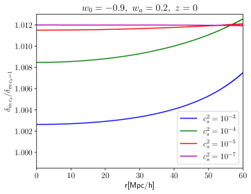
Figure 1: Profiles ratios $\delta_{m\,,c_{s}}/\delta_{m\,,c_{s}=1}$ at $z=0$ for selected values of $c_{s}$. The initial conditions for $\delta_{m}$ are the same in all cases.

4.2 Matter halos

Now we analyze the impact of $c_{s}$ on matter profiles associated with the formation of halos. Starting with the same initial conditions for matter fluctuations at $z_{i}=99$, we show the profiles at very low-$z$. The value of $\delta_{m}\left(r=0,z_{i}\right)$ is chosen to produce a profile that roughly represents virialization overdensities ($\delta_{m}\sim 200$) at $z=0.04$.

In the left panel of figure 2 we can see that lower values of $c_{s}$ enhances matter clustering. For $c_{s}^{2}>10^{-3}$, this enhancement is small when compared to $c_{s}^{2}=1$. For $c_{s}^{2}\leq 10^{-7}$, we verified that $\delta_{m}$ barely changes. The range of variation of the central value of $\delta_{m}$ is substantial, showing that even a small contribution of DE can produce a large modification in the matter fluctuation in the nonlinear regime.

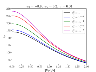
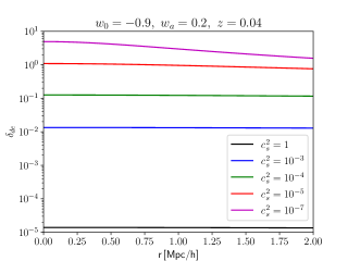
Figure 2: Left panel: impact of DE fluctuations on the nonlinear matter profile at $z=0.04$ for selected values of $c_{s}$. Right panel: profiles of $\delta_{de}$ for the corresponding cases show in the left panel. The initial conditions for matter fluctuations are the same in all cases.

In left panel of figure 2, we show the corresponding profiles of $\delta_{de}$ at $z=0.04$. For $c_{s}^{2}=1$, DE fluctuations stay in the linear regime and are 7 orders of magnitude smaller than matter fluctuations, which can be assumed as homogeneous DE on small scales. In the case of $c_{s}^{2}=10^{-7}$, $\delta_{de}$ can reach few percent of the corresponding matter fluctuations. For the scales under consideration, we see that DE fluctuations become nonlinear for $c_{s}^{2}<10^{-4}$.

In figure 3, we also show the impact of $c_{s}$ on the gravitational potential. In the top panel we show $10^{4}\times\phi$ and in the lower panel the percent differences with respect to the $c_{s}^{2}=1$ case, given by $\Delta_{\phi}=100\times\left(\frac{\phi_{c_{s}}}{\phi_{c_{s}=1}}-1\right)$. As we can see, in the central region, the potential can change about $10\%$ with respect to the homogeneous case ($c_{s}=1$). The impact of $c_{s}$ is also present far away from the center, but is slightly reduced.

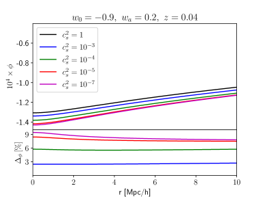
Figure 3: Top panel: Profiles of the potential $\phi$ at $z=0.04$ for selected values of $c_{s}$. Lower panel: percent differences of the potential for various $c_{s}$ with respect to the $c_{s}=1$ case, given by $\Delta_{\phi}=100\times(\phi_{c_{s}}/\phi_{c_{s}=1}-1)$. The initial conditions for $\delta_{m}$ are the same in all cases.

We also check the impact of DE fluctuation of the peculiar matter velocity, which is related to the redshift space-distortion effect. In figure 4 we plot the percent difference of $v_{m}$ with respect to the case with homogeneous DE ($c_{s}=1$), given by $\Delta v_{m}=100\times\left(\frac{v_{mc_{s}}}{v_{mc_{s}=1}}-1\right).$ The vertical dashed line indicates the radius such that $\delta_{m}\simeq 5$. This value roughly indicates the transition between collapsing nonlinear and still expanding linear regions. In the nonlinear regions, DE fluctuations can change $v_{m}$ substantially, in $10-20\%$ range. In the linear regions, the variation with respect to the homegeneous case is only about $3\%$ for the two lowest $c_{s}$ values.

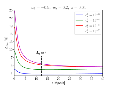
Figure 4: Change of the peculiar matter velocity, $v_{m}$, at $z=0.04$ for selected values of $c_{s}$ with respect to the $c_{s}=1$ case, given by $\Delta v_{m}=100\times\left(\frac{v_{mc_{s}}}{v_{mc_{s}=1}}-1\right)$. The initial conditions for $\delta_{m}$ are the same as those used in figure 2. The vertical dashed-black line shows the region where $\delta_{m}\simeq 5$, which roughly indicates the transition between collapsing and expanding regions.

Phantom negative energy density

In the previous examples, we used $w>-1$ for all the evolution. Now let’s analyze the case of a phantom equation of state. As already noticed in the literature [16, 37, 18], in the limit $c_{s}\rightarrow 0$, positive matter fluctuations will induce negative phantom DE fluctuations, because $\delta_{de}\propto\left(1+w\right)\delta_{m}\,.$ Therefore, it is possible that matter halos can generate $\delta_{de}<-1$, which is associated with the pathological situation of negative total energy in the DE component $\rho_{de}=\bar{\rho}_{de}\left(1+\delta_{de}\right)$.

In figure 5, for $w_{0}=-1.1$ and $w_{a}=0$, we show that this situation is achieved by models with sufficiently low sound speed. Note that, in these examples, $\delta_{m}$ roughly presents virialization values at the central regions. This can be understood as an averaged density contrast for the real halo profile. The changes in the potential with respect to the homogeneous case are smaller and opposite to the non-phantom case, reaching $-2.5\%$ for $c_{s}^{2}=10^{-7}$.

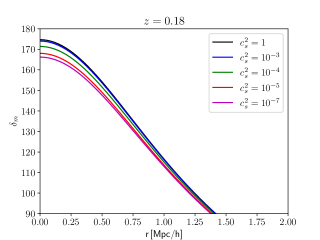
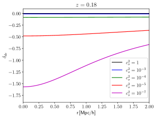
Figure 5: Left panel: $\delta_{m}$ profiles for $w=-1.1$ and selected values of $c_{s}$ at $z=0.18$. Right panel: corresponding $\delta_{de}$ profiles. The initial conditions for $\delta_{m}$ are the same as those used in figure 2.

More realistic halo profiles can have $\delta_{m}\sim 10^{3}$ at the central region. Then, to avoid $\delta_{de}<-1$, larger $c_{s}$ is necessary. In figure 6 we show the profiles for $\delta_{de}$ at $z=0.11$, but now with $\delta_{m}\simeq 1500$ at the center. As can be seen, $\delta_{de}<-1$ is now achieved also for $c_{s}^{2}=10^{-5}$. The DE contrast can be even more negative for lower sound speed values. It is important to note that, having in mind that $\delta_{de}\propto\left(1+w\right)\delta_{m}$, larger values of $c_{s}$will be needed for more negative $w$ to avoid this pathological behavior.

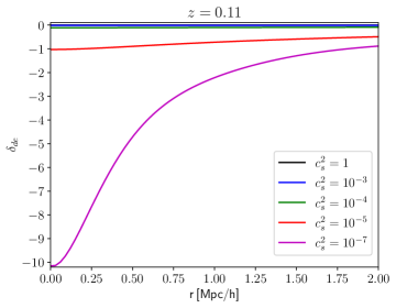
Figure 6: DE profiles for $w=-1.1$ at $z=0.11$ for selected values of $c_{s}$. Here the matter profile is evolved up to $\delta_{m}\simeq 1500$ at the center. In this example, when $c_{s}^{2}<10^{-5}$ we have $\delta_{de}<-1$ around the center of the halo.

The main driver of this pathological behavior is the term $1+w+\left(1+c_{s}^{2}\right)\delta_{de}$ in equation (2.12), which couples the density contrast to the gravitational potential. The corresponding term for matter fluctuations is $1+\delta_{m}$, thus, when $\delta_{m}\rightarrow-1$, the fluctuations decouple from $\phi$, the decrease of $\delta_{m}$ halts, and we always have $\delta_{m}>-1$. However, in general, this coupling term for DE does not vanish when $\delta_{de}\rightarrow-1$, and situations with $\delta_{de}<-1$ can be achieved for sufficiently small $c_{s}$.

At face value, these phenomenological models present pathologies that must be absent in any fundamental theory. Our examples demonstrate that phantom models can not be described as perfect fluids with arbitrarily low $c_{s}$, as in [40]. In practice, many scalar field models with $w<-1$ have no perfect fluid correspondence [41, 42], and dissipative effects may avoid this kind of problem in the nonlinear regime.

4.3 Matter voids

Let us estimate the impact of DE fluctuation on voids. Assuming the same initial conditions as those used in figure 2, but with negative values for $\delta_{m}$, we evolve the profiles up to $z=0.04$. As can be seen in figure 7, the same kind of initial conditions that generate overdensities of nearly virialized halos produce voids with $\delta_{m}\simeq-0.67$ at the central region. The impact of $c_{s}$ on $\delta_{m}$ is much smaller for a void, below $1\%$. The variation of $\delta_{de}$ with $c_{s}$ is also smaller than in the case for halos.

We note that, in the left panel of figure 7, we have $\delta_{de}>0$ for the $c_{s}=1$ case, following the approximate solution $\delta_{de}\propto-\left(1+w\right)\phi/c_{s}^{2}$ for models with relevant pressure support on small scales. For the cases with $c_{s}^{2}<10^{-3}$, we have negative DE fluctuations, following the dust-like approximate solution $\delta_{de}\propto\left(1+w\right)\delta_{m}$.

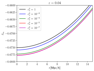
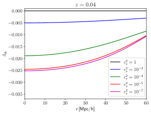
Figure 7: Left panel: impact of DE fluctuations on the nonlinear void matter profile at $z=0.04$ for selected values of $c_{s}$. Right panel: profiles of $\delta_{de}$ for the corresponding cases shown in the left panel. The initial conditions for matter fluctuations are the same in all cases. In the left panel, we focus on more central regions so that the small differences (bellow than $1\%$) in the matter profiles can be visible

Although the impact of DE fluctuation in matter voids is smaller, the change in the potential is similar to what we observed for halos. In the lower panel of 8, we see that $\phi$ can change about $8\%$ with respect to the homogeneous case.

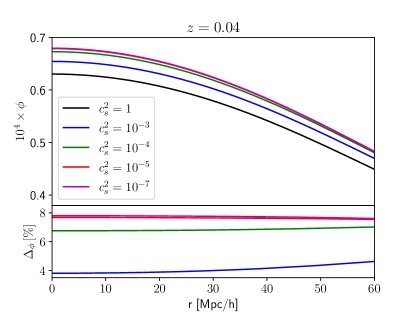
Figure 8: Top panel: Profiles of the potential $\phi$ at $z=0.04$ for selected values of $c_{s}$. Lower panel: percent differences of the potential for various $c_{s}$ with respect to the $c_{s}=1$ case, given by $\Delta_{\phi}=100\times(\phi_{c_{s}}/\phi_{c_{s}=1}-1)$. The initial conditions for $\delta_{m}$ are the same in all cases.

4.4 Local DE EoS

When DE fluctuations are non-negligible, it’s local EoS, defined by

$$w_{c}=\frac{\bar{p}_{de}+\delta p_{de}}{\bar{\rho}_{de}+\delta\rho_{de}}=w+\left(c_{s}^{2}-w\right)\frac{\delta_{de}}{1+\delta_{de}}\,,$$ (4.3)

is expected to vary near a nonlinear structure [14, 16]. With our method to solve for the profiles, we can now analyze how $w_{c}$ changes in space.

For this purpose, we choose $w_{0}=-1$ and $w_{a}=0.2$. This model gives an EoS that is close to $-1$ at low$-z$, but is less negative in the past, allowing DE fluctuation to grow and be present up to now. In this case we have a background similar to $\Lambda$CDM at low redshift, but with still relevant DE fluctuations. In figure 9, we show the profile of $w_{c}$ at $z\simeq 0.026$ using initial conditions for $\delta_{m}$ such that its value at the center roughly represents virialization values. As can be seen, for $c_{s}^{2}<10^{-5}$, the change of the local equation of state with respect to $w$ can be large near the center and still relevant in outer regions. In the case of voids, we have $w_{c}\simeq w$ because the fluctuations of DE are still linear.

In the central regions, the local gravity of the halo dominates over the background expansion. Thus the values of $w_{c}$ shall have a negligible effect on light propagation and particle dynamics. But in the outskirts of halos or in mildly nonlinear structures, it’s possible that departures of $w$ due to DE fluctuations can produce a non-negligible effect. Such impact, however, depends crucially on the actual matter distribution.

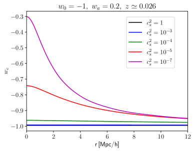
Figure 9: Profiles of the local DE EoS, $w_{c}$, at $z\simeq 0.026$ for selected values of $c_{s}$. The initial conditions for $\delta_{m}$ are the same in all cases and roughly produce virialization overdensities at the central regions at $z\simeq 0.026$.

For phantom DE with low $c_{s}$ in the presence of a matter halo, the local equation of state is ill-defined because $w_{c}$ diverges when $\delta_{de}\rightarrow-1$. For healthy phantom models, it would be possible to find a $c_{s}^{2}$ such that the change in $w_{c}$ is large. For instance, with $w_{0}=-1$, $w_{a}=-0.2$ and $c_{s}^{2}=10^{-5}$ we can find $\delta_{de}\left(r=0\right)\simeq-0.3$ at low-$z$, which produces $w_{c}\left(r=0\right)\simeq-1.57$. However, this kind of model is much more speculative because one would need to fine-tune $c_{s}^{2}$ for each EoS under consideration to avoid $\delta_{de}<-1$.

5 Virialization threshold

In the classical model for the spherical collapse in an EdS universe, the evolution of $\delta_{m}$ can be solved analytically [1, 43]. The top-hat nonlinear density diverges when the shell radius goes to zero, which determines the redshift of collapse $z_{c}$, which, in turn, is used to compute the critical density for collapse, $\delta_{c}$, as the value of the linear evolved contrast at $z_{c}$. As well-known, in EdS model, $\delta_{c}\simeq 1.686$ is independent of redshift and scale. In $\Lambda$CDM model, $\delta_{c}$ is redshift dependent, being slightly smaller than $1.686$ at low $z$ [5, 7]. Smooth dynamical DE, in general, does not change this picture significantly [9].

The threshold density can also be computed for clustering DE models. If $c_{s}$ is negligible on the scales of interest, the DM and DE have the same peculiar velocities, which allows the use of top-hat profiles for both of them [14, 16, 18, 21, 22, 24]. In this case, the model is described as a system of ordinary differential equations, which can be solved numerically up to a certain threshold, e.g., $\delta_{m}\sim 10^{6}$, which then defines $z_{c}$ and $\delta_{c}$. For a detailed discussion about the numerical computation of $\delta_{c}$, see [44, 45, 12].

When solving for the evolution of the radial profile, we observe that the system gets unstable when $\delta_{m}\left(r=0\right)\sim 10^{4}$, which does not allow us to define a reliable threshold for a reasonable redshift range. This is easy to understand with the following example: in the EdS model, starting with $\delta_{m}\left(a_{i}=0.01,r=0\right)=0.01686$, the linear evolution indicates that $\delta_{m}\left(a=1,r=0\right)=1.686$ at $a=1$. Therefore, according to the top-hat spherical collapse model, the nonlinearly evolved contrast will diverge at the origin. This behavior is critical for the evolution of the whole profile, generating spurious oscillations.

Given this difficulty, we will use an alternative method to compute the threshold density, which was proposed in [46] and also developed in [24] for clustering DE. Instead of determining $\delta_{m}^{L}\left(z_{c}\right)$, we will determine the linearly evolved contrast at $z_{\rm v}$, the redshift of virialization. In EdS we have

$$\delta_{{\rm v}}\equiv\bar{\delta}^{L}{}_{m}\left(z_{\rm v}\right)\simeq 1.583\,,$$ (5.1)

$$\Delta_{{\rm v}}\equiv\frac{\rho_{m}}{\bar{\rho}_{m}}=1+\bar{\delta}^{NL}{}_{m}\left(z_{\rm v}\right)\simeq 146.8\,.$$ (5.2)

In the context of non-top-hat profiles, the contrasts with overbar can be understood as volume-averaged quantities. Since at $z_{\rm v}$ the central region of the density contrast has not formally diverged, naturally, the evolution of the entire profile does not present any instability.

As discussed in [24], in the presence of clustering DE, the natural generalization for the virialization threshold is given by

$$\delta_{{\rm v}}\left(z\right)\equiv\bar{\delta}_{{\rm tot}}^{L}\left(z_{v}\right)=\bar{\delta}_{m}^{L}\left(z_{{\rm v}}\right)+\frac{\Omega_{de}\left(z_{{\rm v}}\right)}{\Omega_{m}\left(z_{{\rm v}}\right)}\bar{\delta}_{de}^{L}\left(z_{{\rm v}}\right)$$ (5.3)

and the the virial overdensity by

$$\Delta_{{\rm v}}=\Omega_{m}\left[1+\bar{\delta}_{m}^{NL}\left(z_{{\rm v}}\right)\right]+\Omega_{de}\bar{\delta}_{de}^{NL}\left(z_{{\rm v}}\right)\,.$$ (5.4)

In these expressions, $z_{{\rm v}}$ is the redshift of virialization, determined at the moment that the virial equation for non-conserving mass is satisfied

$$\frac{1}{2M_{{\rm tot}}}\frac{d^{2}M_{{\rm tot}}}{dt^{2}}+\frac{2}{M_{{\rm tot}}R}\frac{dM_{{\rm tot}}}{dt}\frac{dR}{dt}+\frac{1}{R^{2}}\left(\frac{dR}{dt}\right)^{2}+\frac{1}{R}\frac{d^{2}R}{dt^{2}}=0\,,$$ (5.5)

where $M_{{\rm tot}}=M_{\,m}+M_{de}$,

$$M_{m}=\frac{4\pi}{3}R^{3}\bar{\rho}_{m}\left(1+\bar{\delta}_{m}^{NL}\right)\,.$$ (5.6)

and

$$M_{de}=\frac{4\pi}{3}R^{3}\bar{\rho}_{de}\bar{\delta}_{de}^{NL}\left(1+3c_{s}^{2}\right)\,.$$ (5.7)

In the SC model, $M_{m}$ is conserved, but $M_{de}$ is not. For more details about this implementation, see [20, 24].

Now we have to define how to compute the linear and nonlinear volume averaged contrasts, $\bar{\delta}_{m}$ and $\bar{\delta}_{de}$. In the case of a top-hat profile, indicated by $\delta_{m}^{th}\left(t\right)$, we have

$$M_{m}=\frac{4}{3}\pi R^{3}\bar{\rho}_{m}\left(1+\delta_{m}^{th}\left(t\right)\right)\,.$$ (5.8)

Assuming mass conservation within the physical radius $R$, we get the usual continuity equation

$$\dot{\delta}_{m}^{th}+3\left(1+\delta_{m}^{th}\right)\left(\frac{\dot{R}}{R}-\frac{\dot{a}}{a}\right)=0\,,$$ (5.9)

which gives the dependency of $R$ with $\delta_{m}^{th}$

$$\frac{1+\delta_{m}^{th}\left(t\right)}{1+\delta_{m}^{th}\left(t_{i}\right)}=\left(\frac{a\left(t\right)}{a\left(t_{i}\right)}\frac{R\left(t_{i}\right)}{R\left(t\right)}\right)^{1/3}\,.$$ (5.10)

For general profiles, however, we can not analytically determine the relation between $R$ and $\delta_{m}$ because the nonlinear effects and the presence of DE fluctuations change the profile during the evolution. Thus we need to numerically compute the integral

$$M_{m}=4\pi\bar{\rho}_{m}\int_{0}^{R}drr^{2}\left(1+\delta_{m}^{NL}\left(r,t\right)\right)\,,$$ (5.11)

many times at each time of interest to determine the value of $R$ that conserves the mass. Given that the profile implemented is steep, and that it get’s much steeper in the nonlinear regime, the computation of such integral can be numerically unstable in general. To save computational time and for the sake of numerical stability, we determine $R$ using

$$M_{m}=\frac{4\pi}{3}\bar{\rho}_{m}R^{3}\left(1+\delta_{m}^{NL}\left(r_{f},t\right)\right)\,,$$ (5.12)

where $r_{f}\ll\sigma$, so that the profile is nearly constant between $0<r<r_{f}$.

With this simplification, we lose the precise association between $M_{m}$ and the physical scale $R$, but, as we will see, the time-dependent quantities ($\delta_{\rm v}$, $\Delta_{\rm v}$) are determined with good accuracy. In the general case, $\delta_{\rm v}$ and $\Delta_{\rm v}$ would also depend on the mass (or radius) scale. In the examples we will show, we can consider that these quantities are determined for comoving scales, $r$, such that $\delta_{m}$ is roughly constant. From figure 2, we can estimate this is roughly valid for $r<0.25\text{Mpc/h}$. A more detailed analysis of the dependence of the threshold and virialization densities on the scale will be done in a forthcoming paper. For a study about the scale-dependent SC quantities in the presence of linear DE perturbations, see [47]. With this setup, we can check how accurate our model reproduces the classical SC results, see Appendix A.

Finally we determine the impact of $c_{s}^{2}$ on $\delta_{\rm v}$ and $\Delta_{\rm v}$ on small scales. We show results for a non-phantom model ($w_{0}=-0.9$ and $w_{a}=0.2$) and phantom model ($w_{0}=-1.1$ and $w_{a}=-0.2$). We verified that the values for $c_{s}^{2}<10^{-7}$ are very close with those for null sound speed. As expected, for non-phantom DE, in both cases all curves lie in between the ones for $c_{s}^{2}=0$ and $c_{s}^{2}=1$. As can be seen in figure 10, there is an important dependence of $\delta_{{\rm v}}$ with $c_{s}$ at low-$z$.

In the phantom case, there is an interesting trend, namely, for sufficiently small $c_{s}$, $\delta_{{\rm v}}$ decreases with $z$. This happens because low values of $c_{s}$ will induce more negative $\delta_{de}$, which in turn decreases the matter growth and $\delta_{{\rm v}}$. It’s also important to note that, in phantom models, DE becomes important for the background evolution at lower redshifts. Hence, it’s effects are more apparent later than in non-phantom model. Finally, we remark that we restricted $c_{s}^{2}\geq 10^{-3}$ to avoid the negative densities in phantom DE, as discussed in section 4.2.

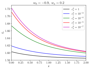
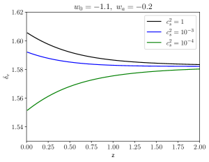
Figure 10: Left panel: evolution of $\delta_{{\rm v}}$ with $z$ for non-phantom models and selected values of $c_{s}$. Right panel: the same, but for phantom models. In this latter case, we restrict the values of $c_{s}$, so that negative densities associated with phantom DE are not present.

6 Conclusions

In this work, we developed a numerical code capable of solving the nonlinear partial equations of the SC model associated with perfect fluids with pressure. This kind of system naturally arises when some clustering component has a scale-dependent growth, as DE with arbitrary sound speed, and cannot be treated by the usual SC methods. Thus we were able to generalize results in the literature that were obtained in the limits of homogeneous DE ($c_{s}=1$) and clustering DE ($c_{s}=0$). Our method shows very good agreement with linear solution in EdS model and with the top-hat SC collapse model for the cases with $c_{s}=1$ and $c_{s}=0$.

We have confirmed that DE fluctuations with $c_{s}=1$ remain very small compared to matter fluctuations, even in the nonlinear regime, as expected in Quintessence and Tachyon models [17, 27]. We also verified that, for $c_{s}<10^{-5}$, DE fluctuations behave as dust and can become nonlinear, also depending on $w$. In this case, the evolution of matter fluctuations is strongly impacted. As a consequence, the virialization threshold, $\delta_{{\rm v}}$, has a substantial increase in non-phantom models and a moderate decrease in phantom healthy models. We also found that, for $c_{s}^{2}<10^{-3}$, the gravitational potential associated with matter halos and voids can change about $4-9\%$ with respect to the $c_{s}^{2}=1$ case. This can be an important observational feature of DE fluctuations [48].

We have shown that phantom DE with low $c_{s}$ can develop a pathological state of negative energy density around matter halos. This can happen for $c_{s}^{2}<10^{-7}$ around virializations overdensities and for $c_{s}^{2}<10^{-5}$ around overdensities $\delta_{m}\sim 10^{3}$. Therefore, in order to avoid negative densities, phantom DE models described by perfect fluids can not have arbitraly low sound speed, such as in model [40]. The specific minimum value of $c_{s}$ that avoids this pathology also depends on $w$. Thus, helthy phantom models demand some fine tune or can not be described by perfect fluids [42].

For the first time, we have explored the dependence of $\delta_{{\rm v}}$ with $c_{s}$. At low redshifts, the departures from the homogeneous case is about $1\%$ for $c_{s}^{2}=10^{-3}$ and increase up to $7\%$ for $c_{s}^{2}=10^{-7}$. As shown in [24], the variation of halo abundances between homogeneous and clustering DE can reach up to $30\%$. Therefore, intermediate values of $c_{s}$ can also present a sizable impact on cluster abundances. Our results are focused on small nonlinear scales. We aim to further develop this code to precisely determine the scale dependence of $\delta_{{\rm v}}$ and implement more realistic profiles.

Our code can be adapted to solve the nonlinear evolution of fluctuations in other cosmological scenarios which present scale-dependent growth of fluctuations, such as warm DM and modified gravity models. The inclusion of bulk viscosity is also possible and models like [23] can be studied beyond the top-hat approximation. A particular interesting application is the case of Ultra Light DM, [49]. In such models, DM naturally has a scale-dependent growth, and small halos develop a core due to “quantum pressure”. Semi-analytical halo abundances of these models have used prescriptions for the collapse threshold proposed in the context homogeneus DE or warm DM [50, 51]. Thus a more detailed semi-analytic study of the nonlinear evolution is still lacking.

Appendix A: Convergence and accuracy tests

Linear evolution

Let’s first analyze the convergence and accuracy of the method in the linear regime. In figure 11 we show the percent error in the $\delta_{m}$ profile at $z=0$, given by

$$E_{m}^{N}\left(r\right)=100\%\times\frac{|\delta_{m}^{EdS}\left(r\right)-\delta_{m}^{N}\left(r\right)|}{\delta_{m}^{EdS}\left(r\right)}\,,$$ (6.1)

where $\delta_{m}^{EdS}$ is the analytical solution, equation (2.16), and $\delta_{m}^{N}$ is the numerical solution for the truncation order $N$. We assume that $\sigma=30\mbox{Mpc/h}$. Here we only show the dependence with $N$, however the map parameter $L_{0}$ is also important because it changes the spatial coverage of the collocation points, which has to be adjusted according to the profile parameters in order to minimize the error. For the present case, $L_{0}=12$ was used.

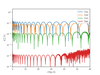
Figure 11: Numerical error profiles for the linear evolution $\delta_{m}$ defined in Eq. (6.1)

As we can see, the error falls with the increase of the truncation order $N$. We observe that $N=60$ minimizes the error within $1\sigma$, which is below $10^{-6}\%$. We also note that the error is cumulative with time. Therefore, for higher redshifts, the error is even smaller. It is also important to note that higher values of $N$ do not necessarily decrease the error. As $N$ grows, more numerical precision is needed to satisfactorily evaluate the base functions at the collocation points. In the algebraic procedure, done with Maple software, the numerical precision can be increased to fulfil this demand. However, when exporting the equations to be integrated with GSL routines written in C language, we are limited to the machine precision, and the errors increase above some $N$. The onset of this limitation can be seen as a noisy error profile for $N=55$ and $N=60$ at large radius. For $N>60$ the error around the origin increases, so we will use $N=60$ in the examples shown in this paper because we mainly interest in the nonlinear evolution, which takes place at more central regions of the profile.

We also verified the accuracy of the numerical procedure comparing the linearly evolved contrasts with the analytical solutions in EdS model for DE Eqs. (2.22) and (2.20), i.e., assuming that the DE is a test field in a matter-dominated universe. For the case with $c_{s}=0$ and assuming $w=-0.9$, the error profile is very similar to what is shown for $\delta_{m}$ in figure 11.

The error for $\delta_{de}$ with $c_{s}=1$ is larger, about a few percent. Probably, this larger imprecision is due to the boundary conditions implemented, Eq. (3.5), which are chosen for better accuracy in models with low $c_{s}$, i.e, they are the same as those for matter. For the results we have shown, the impact of this larger error for the non-negligible sound speed cases is very small because in this case DE perturbations are at least a few orders of magnitude smaller than matter perturbations and barely impact its evolution and quantities used to determine the virialization. We also checked the error in the gravitational potential, which is about the $10^{-5}\%$ order for $N=60$.

Nonlinear evolution

We also compute the error in the nonlinear evolution of $\delta_{m}$ as compared to the analytical solution in EdS. Let us first consider the determination of the critical density threshold at virialization, $\delta_{{\rm v}}$. As discussed earlier, when trying to reproduce the usual threshold for collapse, $\delta_{c}$, severe numerical instabilities arise. Thus, we compare the numerical and analytical determinations of quantities at the virialization time, $z_{{\rm v}}$, in EdS model: $\delta_{{\rm v}}\simeq 1.583$ and $\Delta_{{\rm v}}\simeq 146.8$.

We also compare the evolution of $\delta_{{\rm v}}$ and $\Delta_{{\rm v}}$ provided by our method with the one obtained in the top-hat spherical collapse model in the presence of clustering DE, i.e., for $c_{s}=0$ [24]. In figure 12, we show the percent difference in $\delta_{{\rm v}}$ between the methods is presented for the parameters $w_{0}=-0.9$ and $w_{a}=0.2$. As can be seen, the errors are below $0.1\%$. For $\Delta_{{\rm v}}$ the errors are larger, reaching a few percent for models with DE.

The different errors magnitude for these quantities can be understood as follows. Both of them are determined at the redshift of virialization given by equation 12. The value of $\delta_{{\rm v}}$ is then given by the linear values of the contrast, whereas $\Delta_{{\rm v}}$ by the nonlinear ones. Since $\Delta_{{\rm v}}$ is usually two orders of magnitude larger than $\delta_{{\rm v}}$, thus the same error in $z_{{\rm v}}$ can be amplified by roughly this amount. It’s also important to note that the errors in these quantities depend both on the contrasts evolution and their numerical temporal derivatives, which enter in 12. Moreover, we verified that another numerical implementation for the clustering case, based in Python and with results shown in [12], differs $2-3\%$ from the computations presented here and those from [24], which was implemented in Mathematica. Therefore, it’s important to note that we still lack a sub-percent accurate computation of $\Delta_{{\rm v}}$, which can be used directly in mass functions [52, 53].

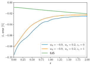
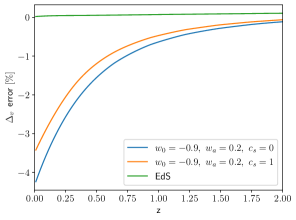
Figure 12: Left panel: Numerical error for $\delta_{{\rm v}}$ when compared to the analytical solution for EdS model and the numerical solution from the top-hat SC model for a model with $w_{0}=-0.9$ and $w_{a}=0.2$ for $c_{s}=1$ and $c_{s}=0$, as presented in [24]. Right panel: the same, but for $\Delta_{{\rm v}}$.

References

- [1] J. E. Gunn and J. R. I. Gott, On the infall of matter into cluster of galaxies and some effects on their evolution, Astrophys. J. 176 (1972) 1–19.
- [2] W. H. Press and P. Schechter, Formation of galaxies and clusters of galaxies by selfsimilar gravitational condensation, Astrophys. J. 187 (1974) 425–438.
- [3] R. K. Sheth, H. J. Mo, and G. Tormen, Ellipsoidal collapse and an improved model for the number and spatial distribution of dark matter haloes, Mon. Not. Roy. Astron. Soc. 323 (2001) 1, [astro-ph/9907024].
- [4] O. Lahav, P. B. Lilje, J. R. Primack, and M. J. Rees, Dynamical effects of the cosmological constant, Mon. Not. Roy. Astron. Soc. 251 (1991) 128–136.
- [5] P. B. Lilje, Abundance of Rich Clusters of Galaxies: A Test for Cosmological Parameters, Astrophysical Journal Letters 386 (Feb., 1992) L33.
- [6] V. R. Eke, S. Cole, and C. S. Frenk, Using the evolution of clusters to constrain Omega, Mon. Not. Roy. Astron. Soc. 282 (1996) 263–280, [astro-ph/9601088].
- [7] T. Kitayama and Y. Suto, Semianalytical predictions for statistical properties of x-ray clusters of galaxies in cold dark matter universes, Astrophys. J. 469 (1996) 480, [astro-ph/9604141].
- [8] L.-M. Wang and P. J. Steinhardt, Cluster abundance constraints on quintessence models, Astrophys. J. 508 (1998) 483–490, [astro-ph/9804015].
- [9] N. N. Weinberg and M. Kamionkowski, Constraining dark energy from the abundance of weak gravitational lenses, Mon. Not. Roy. Astron. Soc. 341 (2003) 251, [astro-ph/0210134].
- [10] W. J. Percival, Cosmological structure formation in a homogeneous dark energy background, Astron. Astrophys. 443 (2005) 819, [astro-ph/0508156].
- [11] E. Abdalla et. al., Cosmology intertwined: A review of the particle physics, astrophysics, and cosmology associated with the cosmological tensions and anomalies, JHEAp 34 (2022) 49–211, [arXiv:2203.0614].
- [12] R. C. Batista, A Short Review on Clustering Dark Energy, Universe 8 (2021), no. 1 22, [arXiv:2204.1234].
- [13] W. Cardona and M. A. Sabogal, Holographic energy density, dark energy sound speed, and tensions in cosmological parameters: and , arXiv:2210.1333.
- [14] D. F. Mota and C. van de Bruck, On the spherical collapse model in dark energy cosmologies, Astron. Astrophys. 421 (2004) 71–81, [astro-ph/0401504].
- [15] N. J. Nunes and D. F. Mota, Structure formation in inhomogeneous dark energy models, Mon. Not. Roy. Astron. Soc. 368 (2006) 751–758, [astro-ph/0409481].
- [16] L. Abramo, R. Batista, L. Liberato, and R. Rosenfeld, Structure formation in the presence of dark energy perturbations, JCAP 0711 (2007) 012, [arXiv:0707.2882].
- [17] D. F. Mota, D. J. Shaw, and J. Silk, On the magnitude of dark energy voids and overdensities, 0709.2227.
- [18] P. Creminelli, G. D’Amico, J. Norena, L. Senatore, and F. Vernizzi, Spherical collapse in quintessence models with zero speed of sound, JCAP 1003 (2010) 027, [arXiv:0911.2701].
- [19] N. Wintergerst and V. Pettorino, Clarifying spherical collapse in coupled dark energy cosmologies, Phys. Rev. D82 (2010) 103516, [arXiv:1005.1278].
- [20] T. Basse, O. E. Bjaelde, and Y. Y. Y. Wong, Spherical collapse of dark energy with an arbitrary sound speed, JCAP 1110 (2011) 038, [arXiv:1009.0010].
- [21] R. Batista and F. Pace, Structure formation in inhomogeneous Early Dark Energy models, JCAP 1306 (2013) 044, [arXiv:1303.0414].
- [22] F. Pace, R. C. Batista, and A. Del Popolo, Effects of shear and rotation on the spherical collapse model for clustering dark energy, Mon.Not.Roy.Astron.Soc. 445 (2014) 648, [arXiv:1406.1448].
- [23] H. Velten, T. R. P. Caramês, J. C. Fabris, L. Casarini, and R. C. Batista, Structure formation in a viscous CDM universe, Phys.Rev. D90 (2014), no. 12 123526, [arXiv:1410.3066].
- [24] R. C. Batista and V. Marra, Clustering dark energy and halo abundances, JCAP 11 (2017) 048, [arXiv:1709.0342].
- [25] C. Heneka, D. Rapetti, M. Cataneo, A. B. Mantz, S. W. Allen, and A. von der Linden, Cold dark energy constraints from the abundance of galaxy clusters, Mon. Not. Roy. Astron. Soc. 473 (2018), no. 3 3882–3894, [arXiv:1701.0731].
- [26] F. Pace and C. Schimd, Tidal virialization of dark matter haloes with clustering dark energy, JCAP 03 (2022), no. 03 014, [arXiv:2201.0419].
- [27] M. P. Rajvanshi and J. S. Bagla, Non-linear spherical collapse in tachyon models, and a comparison of collapse in tachyon and quintessence models of dark energy, Class. Quant. Grav. 37 (2020), no. 23 235008, [arXiv:2003.0764].
- [28] C.-C. Chang, W. Lee, and K.-W. Ng, Spherical Collapse Models with Clustered Dark Energy, Phys. Dark Univ. 19 (2018) 12–20, [arXiv:1711.0043].
- [29] J. Dakin, S. Hannestad, T. Tram, M. Knabenhans, and J. Stadel, Dark energy perturbations in n-body simulations, JCAP 08 (2019) 013, [arXiv:1904.0521].
- [30] F. Hassani, J. Adamek, M. Kunz, and F. Vernizzi, k-evolution: a relativistic n-body code for clustering dark energy, JCAP 12 (2019) 011, [arXiv:1910.0110].
- [31] J. A. S. Lima, V. Zanchin, and R. H. Brandenberger, On the newtonian cosmology equations with pressure, Mon. Not. Roy. Astron. Soc. 291 (1997) L1–L4, [astro-ph/9612166].
- [32] M. Manera and D. F. Mota, Cluster number counts dependence on dark energy inhomogeneities and coupling to dark matter, Mon. Not. Roy. Astron. Soc. 371 (2006) 1373, [astro-ph/0504519].
- [33] F. Pace, J. C. Waizmann, and M. Bartelmann, Spherical collapse model in dark energy cosmologies, arXiv:1005.0233 [astro-ph.CO] (2010).
- [34] M. Chevallier and D. Polarski, Accelerating universes with scaling dark matter, Int. J. Mod. Phys. D10 (2001) 213–224, [gr-qc/0009008].
- [35] E. V. Linder and R. N. Cahn, Parameterized Beyond-Einstein Growth, Astropart.Phys. 28 (2007) 481–488, [astro-ph/0701317].
- [36] L. Abramo, R. Batista, L. Liberato, and R. Rosenfeld, Physical approximations for the nonlinear evolution of perturbations in inhomogeneous dark energy scenarios, Phys.Rev. D79 (2009) 023516, [arXiv:0806.3461].
- [37] D. Sapone, M. Kunz, and M. Kunz, Fingerprinting dark energy, Phys. Rev. D80 (2009) 083519, [arXiv:0909.0007].
- [38] M. A. Alcoforado, R. F. Aranha, W. O. Barreto, and H. P. de Oliveira, New numerical framework for the generalized baumgarte-shapiro-shibata-nakamura formulation: The vacuum case for spherical symmetry, Phys. Rev. D 104 (2021), no. 8 084065, [arXiv:2105.0909].
- [39] J. P. Boyd, Chebyshev and Fourier Spectral Methods. Dover Publications, 2001.
- [40] P. Creminelli, G. D’Amico, J. Norena, and F. Vernizzi, The effective theory of quintessence: the w<-1 side unveiled, JCAP 0902 (2009) 018, [arXiv:0811.0827].
- [41] O. Pujolas, I. Sawicki, and A. Vikman, The Imperfect Fluid behind Kinetic Gravity Braiding, JHEP 11 (2011) 156, [arXiv:1103.5360].
- [42] I. Sawicki and A. Vikman, Hidden Negative Energies in Strongly Accelerated Universes, Phys. Rev. D87 (2013), no. 6 067301, [arXiv:1209.2961].
- [43] T. Padmanabhan, Structure Formation in the Universe. Cambridge University Press, 1993.
- [44] D. Herrera, I. Waga, and S. E. Jorás, Calculation of the critical overdensity in the spherical-collapse approximation, Phys. Rev. D 95 (2017), no. 6 064029, [arXiv:1703.0582].
- [45] F. Pace, S. Meyer, and M. Bartelmann, On the implementation of the spherical collapse model for dark energy models, JCAP 10 (2017) 040, [arXiv:1708.0247].
- [46] S. Lee and K.-W. Ng, Spherical collapse model with non-clustering dark energy, JCAP 1010 (2010) 028, [arXiv:0910.0126].
- [47] T. Basse, O. E. Bjaelde, S. Hannestad, and Y. Y. Y. Wong, Confronting the sound speed of dark energy with future cluster surveys, arXiv:1205.0548.
- [48] F. Hassani, J. Adamek, and M. Kunz, Clustering dark energy imprints on cosmological observables of the gravitational field, Mon. Not. Roy. Astron. Soc. 500 (2020), no. 4 4514–4529, [arXiv:2007.0496].
- [49] E. G. M. Ferreira, Ultra-light dark matter, Astron. Astrophys. Rev. 29 (2021), no. 1 7, [arXiv:2005.0325].
- [50] D. J. E. Marsh and J. Silk, A Model For Halo Formation With Axion Mixed Dark Matter, Mon. Not. Roy. Astron. Soc. 437 (2014), no. 3 2652–2663, [arXiv:1307.1705].
- [51] D. J. E. Marsh, Warmandfuzzy: the halo model beyond cdm, arXiv:1605.0597.
- [52] W. A. Watson, I. T. Iliev, A. D’Aloisio, A. Knebe, P. R. Shapiro, and G. Yepes, The halo mass function through the cosmic ages, Mon. Not. Roy. Astron. Soc. 433 (2013) 1230, [arXiv:1212.0095].
- [53] G. Despali, C. Giocoli, R. E. Angulo, G. Tormen, R. K. Sheth, G. Baso, and L. Moscardini, The universality of the virial halo mass function and models for non-universality of other halo definitions, Mon. Not. Roy. Astron. Soc. 456 (2016), no. 3 2486–2504, [arXiv:1507.0562].