ProSiT! Latent Variable Discovery with PROgressive SImilarity Thresholds

Tommaso Fornaciari
Italian National Police
&Dirk Hovy
Bocconi University
&Federico Bianchi
Stanford University
tommaso.fornaciari@poliziadistato.it dirk.hovy@unibocconi.it fede@stanford.edu

Abstract

The most common ways to explore latent document dimensions are topic models and clustering methods. However, topic models have several drawbacks: e.g., they require us to choose the number of latent dimensions a priori, and the results are stochastic. Most clustering methods have the same issues and lack flexibility in various ways, such as not accounting for the influence of different topics on single documents, forcing word-descriptors to belong to a single topic (hard-clustering) or necessarily relying on word representations. We propose PROgressive SImilarity Thresholds - ProSiT, a deterministic and interpretable method, agnostic to the input format, that finds the optimal number of latent dimensions and only has two hyper-parameters, which can be set efficiently via grid search. We compare this method with a wide range of topic models and clustering methods on four benchmark data sets. In most setting, ProSiT matches or outperforms the other methods in terms six metrics of topic coherence and distinctiveness, producing replicable, deterministic results.

1 Introduction

Latent variable models are essential for data exploration and are commonly used in social science and business applications. However, the most common methods used to explore these models, topic models and clustering, come with a set of drawbacks, chief among them their stochastic nature. This makes results hard to replicate precisely, as they require constant interpretation. In this paper, we instead propose a latent variable discovery method that produces deterministic results.

Topic models, such as latent Dirichlet allocation (LDA) Blei et al. (2003), rely on a number of topics that are provided a priori, refining their initial random guesses to establish probability distribution iteratively. This approach guarantees that the final state improves over the initial one in terms of topic quality, but the method is vulnerable to local optima. This problem can be mitigated by initializing several models and picking the most useful/interpretable solution. Selection usually relies on coherence measures that estimate the topics’ reliability. However, the method also expects the user to provide the number of topics as a parameter. Therefore the probability of finding good results depends on previous domain knowledge about the data set - which is often an unreasonable expectation. In these cases, it is difficult to interpret or justify the resulting topics theoretically, as they depend on an arbitrary starting point. Moreover, since each model’s random initialization will provide slightly different results, these results are debatable.

Clustering methods, another popular choice for exploring latent document dimensions, similarly rely on the number of latent dimensions as input and their random initialization. For example, $K$ -Means Sculley (2010) can extract topics from groups of documents identified by minimizing the distance between the documents’ representations. The procedure partitions the vectors space in Voronoi cells, where each document exclusively contributes to the identification of a single cluster Burrough et al. (2015). However, in many scenarios, the distinction between clusters/topics is nuanced, and we expect to find borderline texts that can be connected to different topics, which should not, in turn, be artificially forced to belong to a unique cluster.

To overcome these limitations, we propose ProSiT, a deterministic and interpretable latent variable discovery algorithm that is entirely reproducible. ProSiT is agnostic to the input space (embeddings, discrete textual, and even non-textual features), allowing for flexible use and inheriting the properties of the input representations of whatever nature. For example, with documents encoded by a multi-lingual model, the identified topics will also be multi-lingual.

ProSiT is entirely data-driven and does not depend on any guess or random initialization. Instead, as the name suggests, it relies on the similarity between texts, i.e., their distances in the vector space. The only theoretical assumption we make is that documents treating similar topic(s) will contain similar words, and therefore will be in proximate regions of the vector space.In geometric terms, we assume the topic’s convexity in the vector space, which implies that the distance between points represents their degree of similarity.

We evaluate ProSiT on four commonly used data sets against eight common and State-Of-The-Art latent variable discovery methods. We evaluate the performance with six standard metrics of latent topic coherence and distinctiveness. We find that ProSiT is always comparable and often superior to State-Of-The-Art methods but requires fewer parameters and no prior selection of latent components.

Contributions

We propose ProSiT, a novel algorithm for latent variable discovery. It is interpretable, deterministic, input agnostic, fuzzy, computationally efficient, and effective. We release ProSiT as a PyPi package. The documentation can be found on GitHub.¹¹1https://github.com/fornaciari/prosit

2 ProSiT

ProSiT takes as input a corpus of documents. The algorithm has two main steps: 1) identifying the latent variables (from here on: topics) and 2) extracting words describing these topics.

ProSiT is efficient for inductive learning: once trained, the topics are represented as points in the same vector space as the training documents. To evaluate unseen documents is as simple as computing their distance from the topics coordinates. The only requirement for new documents is that they are represented in the same vector space as the training data.

2.1 Step 1: Finding topics

The first step is an iterative process that identifies several potential topic sets. The number of topics is data-driven, rather than decided a priori. ProSiT uses different degrees of similarity between groups of documents to determine whether they belong to a topic. These similarity levels are determined by a threshold, which changes at each iteration step and follows a hyperbolic curve. A parameter we call $\alpha$ tunes the slope of this curve.

Formally, we assume a set of documents $D$ . Each document is represented in two ways: as a $d$ -dimensional vector $m$ (continuous or sparse), and as a list of strings $s$ , representing the (pre-processed) document with space-separated words.

We use the matrix $M$ over every document vector $m$ to determine the topics and $S$ over every string representation $s$ to extract the topic descriptors.

We set a similarity threshold $\alpha$ and iterate over $M$ with the following procedure until it stops at the smallest number of topics found:

1.

removing any (possible) duplicated vectors to prevent topics being affected by repeated documents. This step could seem unnecessary, but many corpora contain repeated texts. Since ProSiT models topics as clusters of their associated documents’ average representation, removing duplicates reduces the impact of repeated documents on topic identification.
2.

computing the cosine similarity between all documents in $M$ :

$C=\frac{MM^{\top}}{\left\lVert M\right\rVert\left\lVert M^{\top}\right\rVert}$ (1)

The norms are computed row-wise and multiplied as column and row vectors, respectively. The resulting matrix $C$ is a square, symmetric similarity matrix over the unique input documents.
3.

mapping each data point to the set of all its neighbors (including itself), that is, the set of points more similar than the threshold $\alpha$ . The output of this procedure is a list of redundant sets. However, it also identifies isolated instances too far from others, resulting in a singleton set. Both situations are simplified in Figure 1.
4.

removing the groups that are repeated subsets of other groups;
5.

computing the groups’ centroids, i.e., the documents’ average vector;
6.

assigning isolated instances (outliers) to the group having the closest centroid;
7.

recomputing the cluster centroids, including the outliers in the groups to which they were assigned.
8.

re-starting the iteration, using the centroids as new data points (keeping track of the original data points associated with these centroids)

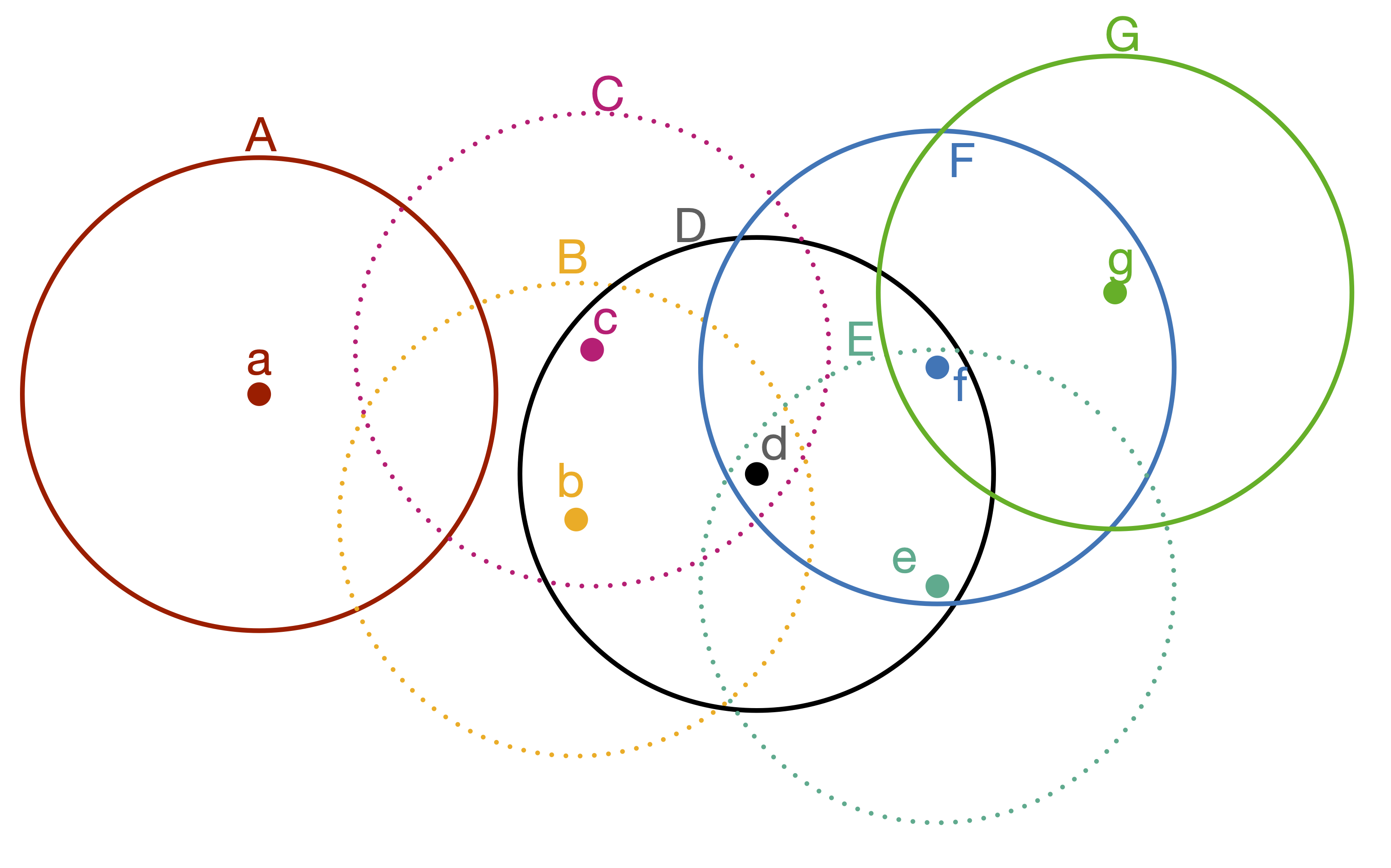
Refer to caption — Figure 1: Examples of data points (lowercase letters) and the relative neighbourhood areas (uppercase letters), determined by $\alpha$ . The dotted lined represent sets of neighbors that are subsets of other sets.

Similarly to agglomerative hierarchical clustering, each document is initially considered its own topic. The number of topics is reduced by iteratively collapsing the documents together. However, ProSiT and agglomerative hierarchical clustering differ substantially. In the latter, pairs of instances are iteratively joined, creating a tree that is representable by dendrograms and in which each instance belongs to one cluster only. In ProSiT, as shown in Figure 1, we create sets of instances lying within a similarity threshold, where overlap between sets is allowed. Therefore, a given instance can contribute to the centroid computation of more than one cluster, leading to smoother topic representations.

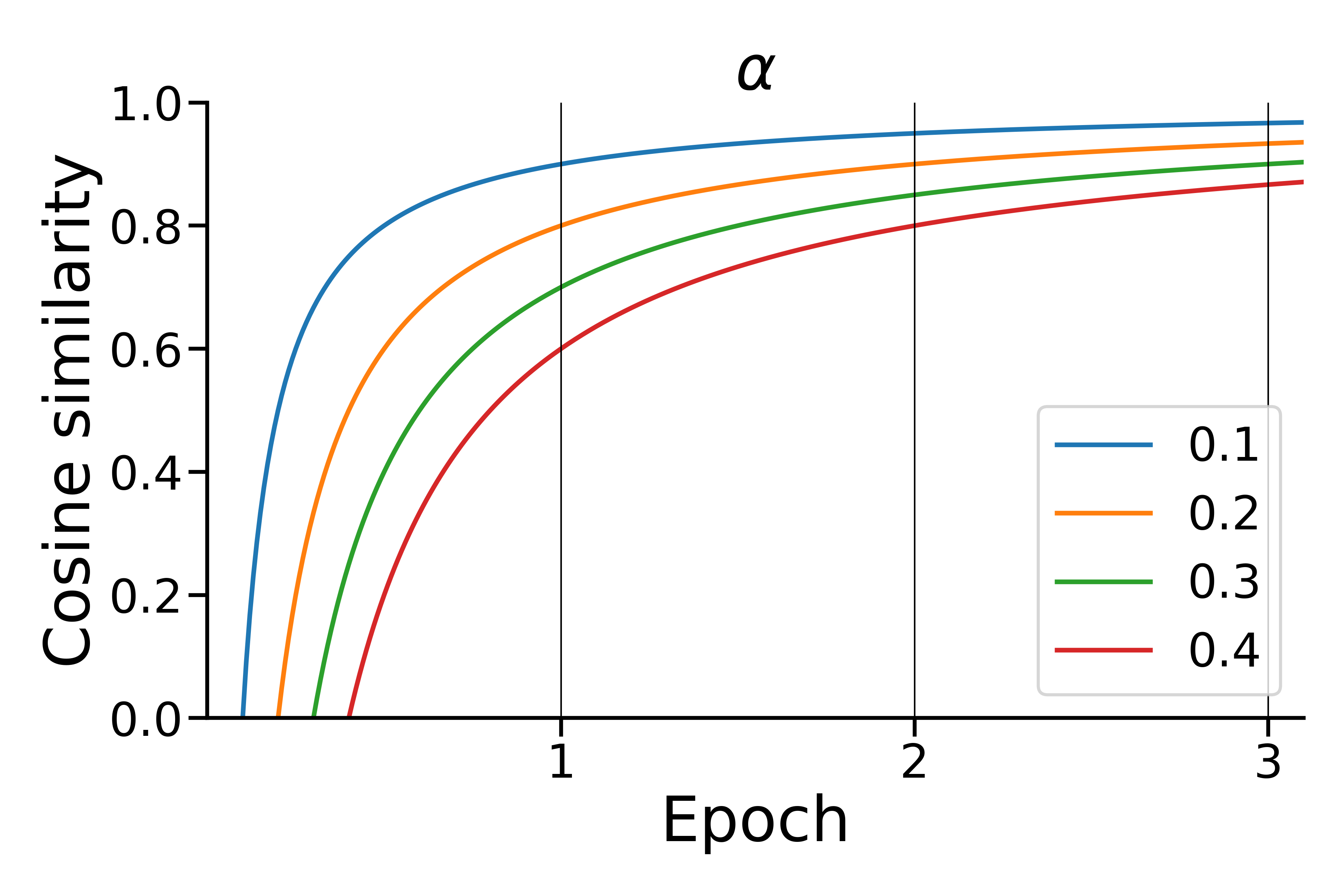
However, there is a problem: Iteratively averaging document vectors pushes the resulting centroids towards the mean of means, i.e., the global centroid of the entire data set. To prevent the document representations from collapsing in one point, in ProSiT we set an increasingly higher cosine similarity threshold ( $CST$ ) at every training iteration $iter$ according to a hyperbolic function

CST=\frac{iter-\alpha}{iter}

(2)

whose slope depends on the $\alpha$ parameter.

Since the thresholds are cosine similarity values, the maximal value is 1. We will therefore want an $\alpha$ value close to 0. Figure 2 shows the hyperbolic curve for various values of $\alpha$ .

ProSiT does not require the number of topics/clusters as an input: They emerge from the process. Topics correspond to the number of clusters identified at each iteration, which become progressively lower until the algorithm reaches convergence. The convergence is reached when all the computed centroids are farther (or less similar) from each other than the threshold, $\alpha$ .

Since the topics are represented as points in the documents’ vector space, we can compute the affinity between any (unseen) document and each topic in terms of distance, similarly to LDA, which measures the topics’ presence in each document.

2.2 Step 2: Selecting topic descriptors

Once ProSiT has identified a set of topics, the second step consists of selecting the documents that best represent each topic and extracting the most representative terms from them. While it is possible to extract the descriptors at every iteration (each corresponding to a different number of topics), for ease of exposition, we show the results for topics ranging between 5 and 25.

In hard clustering methods, identifying the documents that provide the descriptors is straightforward, as every document belongs to a unique topic. In our case, though, we consider the continuous distance between documents and topics so that documents can be associated with several topics with different distance levels. We are interested in selecting the most representative documents, i.e., the closest ones to the topic centroids. To achieve this, we use another threshold, $\beta$ , to define how close to the topics a document should be for the topics to be used for descriptors. $\beta$ describes $n$ percent documents closest to each topic centroid, ranging from 0 to 1 (where 1 means the whole data set).

Once we have selected the set of documents that are most representative of each topic, we extract the descriptors using the information gain (IG) Forman et al. (2003) value, computed for each topic. IG measures the entropy of features selected from some instances belonging to different classes. It is usually used for feature selection from instances in binary classification tasks. Here we propose an original use of IG in a multi-class scenario, where the topics represent the classes. We rank the terms according to their IG (i.e., probability of belonging to a topic) and select the top $n$ words. This procedure, similarly to the document-topics’ affinity, can measure the affinity between words and topics.

3 Experimental Settings

3.1 Data sets

We test ProSiT on four data sets, two with long documents and two with short documents. For long documents, we use the Reuters and Google News data sets,²²2The Reuters data set can be found at https://www.nltk.org/book/ch02.html. which have previously been used by Sia et al. (2020) and Qiang et al. (2020), respectively. For short documents, we use Wikipedia abstracts from DBpedia,³³3The abstracts can be found at https://wiki.dbpedia.org/downloads-2016-10. the same data set used in by Bianchi et al. (2021b), to which we refer as Wiki20K, and a tweet data set, used for topic models by Qiang et al. (2020). Wiki20K Bianchi et al. (2021b) contains Wikipedia abstracts filtered to consist of only the 2,000 most frequent words of the vocabulary. Tweet and Google News are standard data sets in the community and were released by Qiang et al. (2020); both data sets have been preprocessed (e.g., stop words have been removed). Table 1 contains descriptive statistics for the data sets. We use a small vocabulary size, which is desirable for most Topic Models scenarios, where including extremely-low frequency terms would result in a too fine-grained number of topics.

Data set	Docs	Vocab.	M. words	pre-p.
Reuters	10,788	949	130.11	55.02
Google News	10,950	2,000	191.98	68.00
Wiki20K	20,000	2,000	49.82	17.44
Tweets2011	2,472	5098	8.56	8.56

Table 1: Corpora statistics, with vocabulary size and mean words with and without pre-processing.

3.2 Metrics

We evaluate the topics with four metrics for coherence and two for distinctiveness. First, we use standard coherence measures, that is $C_{V}$ and Normalized Pointwise Mutual Information (NPMI) Röder et al. (2015). Also, we consider the Rank-Biased Overlap (RBO) Webber et al. (2010), a discrete measure of overlap between sequences. We also use the inverted RBO (IRBO) score, that is 1 - RBO Bianchi et al. (2021a). This score describes how different the different topics are on average. Lastly, similarly to the approach of Ding et al. (2018), we use an external word embedding-based coherence measure (WECO) to compute the coherence on an external domain. This metric computes the average pairwise similarity of the words in each topic and averages the results. We use the standard GoogleNews word embedding commonly used in the literature Mikolov et al. (2013).

Concerning the distinctiveness, that is, how clearly the topics differentiate from each other, following Mimno and Lee (2014) we measure Topic Specificity (TS) and Topic Dissimilarity (TD). The first is the average Kullback-Leibler divergence Kullback and Leibler (1951) from each topic’s conditional distribution to the corpus distribution; the second is based on the conditional distribution of words across different topics.

While we discuss the outcomes of all metrics, for space constraints, we only show the results of $C_{V}$ , reporting the whole results in Appendix.

3.3 Baselines

We compare ProSiT with two groups of models, differing by the text representations they require as input: embeddings or sparse count features. ProSiT allows us to use each of them.

All comparison methods require the number of latent topics as an a-priori input parameter. We evaluate their performance for inputs of 5, 10, 15, 20, and 25 topics to show a defined range. However, recall that ProSiT does not take the number of topics as input but instead identifies them automatically. Therefore, we also evaluate the other models on those numbers of topics that ProSiT finds.

Input	SBERT embeddings			BoW
Topics	ProSiT	CTM	ZSTM	ProSiT	Agg.	Agg.+KM	KM	N-PLDA	LDA	DBScan
5	0.7229*	0.5697	0.5907	0.7508*	0.5258	0.5133	0.5145	0.6438	0.5185
6		0.5626	0.5638*	0.7387*	0.5468	0.5548	0.5157	0.5337	0.5202
7	0.7617*	0.6299	0.5933		0.5465	0.5316	0.5312	0.5997*	0.5303
8		0.6795*	0.6338	0.6643*	0.5848	0.5601	0.5236	0.655	0.5061
9	0.6941*	0.6843	0.6833	0.6339	0.5784	0.5617	0.5628	0.6398*	0.5069
10		0.667	0.7055*		0.5536	0.5528	0.5154	0.6436*	0.5063
11	0.6449	0.6701	0.6798*		0.5447	0.5462	0.5009	0.6456*	0.5126
13	0.6688	0.6302	0.6798*	0.6461	0.5352	0.5257	0.5438	0.6516*	0.5234
15		0.6698	0.692*	0.6667*	0.5403	0.5353	0.5342	0.6195	0.5256
16		0.6743*	0.6647	0.6668*	0.5269	0.535	0.5333	0.6515	0.522
17	0.6384	0.6681*	0.6291		0.5388	0.5449	0.5431	0.64*	0.5347
20		0.6312	0.6355*		0.5274	0.5315	0.5475	0.6387*	0.5205	0.3726
21	0.6244	0.6366*	0.6348		0.5404	0.5433	0.553	0.6171*	0.5122
25		0.6424	0.6644*		0.5515	0.552	0.5716	0.6576*	0.5202

Table 2: Coherence values for Reuters data set. Bold: best group performance. *: best row performance. ProSiT columns differ by input formats.

In the first group, we consider contextualized topic models (Bianchi et al., 2021a, CTM) and ZeroShot topic models (Bianchi et al., 2021b, ZSTM). They introduce the use of contextual embeddings in topic models. Both rely on sentence-BERT (Reimers and Gurevych, 2019, SBERT) embeddings.

Second, we compare with models that take frequency-based bag-of-words (BoW) input representations. These are agglomerative hierarchical cluster analysis (Agg.) (Maimon and Rokach, 2010, Agg), K-means (KM) (Sculley, 2010, KM), K-means initialized with the agglomerative clustering centroids (Agg.+KM), Latent Dirichlet Allocation (LDA) Blei et al. (2003), neural-ProdLDA (N-PLDA) (Srivastava and Sutton, 2017, NPLDA) and DBScan (DBScan) Schubert et al. (2017).

Neural-ProdLDA is a novel, state-of-the-art method, while LDA, agglomerative clustering and K-means are well-known and widely used techniques. Similarly to ProSiT, DBScan discovers the number of topics as part of the training. Since the two methods tend to discover a different number of topics, a direct comparison is not possible. However, we show the DBScan performance for positioning purposes.

With the same constraint, we compare with Top2Vec Angelov (2020), a recent method that jointly considers document and word representations. We feed ProSiT with the same input (Doc2vec embeddings) and we show the performance, even though the number of topics differ. Lastly, for positioning purposes, we show (for the two data sets considered in the released code) the performance of the procedure proposed by Sia et al. (2020), that relies on word representation and creates clusters using several algorithms (Section A.6).

3.4 ProSiT tuning

ProSiT’s effectiveness depends on the choice of $\alpha$ and $\beta$ . We select them via grid search, evaluating the performance with the metrics mentioned above. In this study, we found the optimal values ranged from $0.02$ to $1\text{\times}{10}^{-06}$ for $\alpha$ and from $0.2$ to $0.03$ for $\beta$ . The small values for $\alpha$ here are not surprising, as the texts can be projected into very dense regions of the vector space. In particular, Ethayarajh (2019) “find that BERT embeddings occupy a narrow cone in the vector space, and this effect increases from the earlier to later layers”, as is also pointed out by Rogers et al. (2020). We report the models with the best $C_{V}$ , obtained through grid search. The other metrics are taken from those selected models.

Input	SBERT embeddings			BoW
Topics	ProSiT	CTM	ZSTM	ProSiT	Agg.	Agg.+KM	KM	N-PLDA	LDA	DBScan
5		0.762	0.7831*	0.8073	0.8648*	0.8648	0.8648	0.7399	0.6805
6	0.7454	0.723	0.7938*	0.8047	0.858*	0.858	0.858	0.7752	0.6529
7	0.686	0.65	0.8064*		0.8647*	0.8647	0.8647	0.7369	0.6702
10		0.704	0.7704*		0.8317	0.8436	0.8524*	0.72	0.6529
11		0.6741	0.7122*	0.7166	0.8368	0.8335	0.8402*	0.6677	0.6594
12	0.7503*	0.688	0.6911		0.8484*	0.8454	0.8294	0.7186	0.652
13	0.7111	0.6952	0.7413*	0.787	0.8557	0.8582*	0.8508	0.7118	0.7152
15		0.7057	0.7639*		0.8587	0.8609*	0.8587	0.7087	0.6983
20	0.6445	0.7101	0.7137*		0.8182	0.8168	0.8322*	0.6672	0.6295
22	0.667	0.6986	0.706*	0.7372	0.8179	0.8167	0.8269*	0.7264	0.6268
25		0.6954*	0.6813	0.7316	0.8202	0.8194	0.8267*	0.6497	0.6644

Table 3: Coherence values for Google News data set. Bold: best group performance. *: best row performance. ProSiT columns differ by input formats.

Input	SBERT embeddings			BoW
Topics	ProSiT	CTM	ZSTM	ProSiT	Agg.	Agg.+KM	KM	N-PLDA	LDA	DBScan
5		0.6109*	0.6026	0.7339*	0.6605	0.6812	0.6087	0.6241	0.552
8	0.7223*	0.6623	0.669	0.7623*	0.7041	0.7154	0.6534	0.6896	0.5276
10		0.7301*	0.6843		0.7243*	0.7075	0.6744	0.7027	0.5537
13	0.7658*	0.7268	0.7295	0.7274*	0.7272	0.7062	0.6969	0.7039	0.5596
15	0.7308	0.7404*	0.7246		0.7153	0.6859	0.7058	0.7627*	0.5459
18		0.752	0.7538*		0.7173*	0.6946	0.704	0.702	0.5573	0.6302
20		0.7373*	0.7314		0.7241	0.6999	0.6474	0.7592*	0.5742
23	0.7349	0.73	0.741*	0.7604*	0.7294	0.7153	0.6917	0.7214	0.5842
24		0.746*	0.7339	0.752*	0.7286	0.7179	0.6835	0.7284	0.6018
25	0.7491*	0.7448	0.7361		0.7303	0.72	0.6731	0.7649*	0.5885

Table 4: Coherence values for Wiki20K data set. Bold: best group performance. *: best row performance. ProSiT columns differ by input formats.

Input	SBERT embeddings			BoW
Topics	ProSiT	CTM	ZSTM	ProSiT	Agg.	Agg.+KM	KM	N-PLDA	LDA	DBScan
5		0.4553*	0.3935		0.702	0.7022*	0.585	0.3761	0.4372
6		0.4115*	0.3929	0.7153*	0.6622	0.6533	0.6809	0.3811	0.3966
10	0.5909*	0.4242	0.4086		0.6675*	0.6472	0.6395	0.398	0.4119
11		0.4164	0.5114*	0.5132	0.6447*	0.6304	0.6309	0.4018	0.397
15		0.4481	0.4593*		0.6584*	0.6536	0.6379	0.4451	0.3887
19	0.5788*	0.4871	0.4582		0.6541	0.6604*	0.6321	0.4135	0.403
20		0.5151*	0.4823		0.6594	0.6621	0.6896*	0.464	0.3978
23		0.4859*	0.4594		0.6732*	0.6706	0.6522	0.425	0.428	0.5193
25		0.4782*	0.4499		0.6786	0.6788	0.6859*	0.519	0.4023

Table 5: Coherence values for Tweet data set. Bold: best group performance. *: best row performance. ProSiT columns differ by input formats.

4 Results

Tables 2 to 5 show the coherence values for the four data sets. Vertical lines separate different sets of results, grouped according to the kind of input provided to the models, as pointed out in Section 3.3. ProSiT’s outcomes are reported in the darkest columns and compared with the columns to their right. The results in bold underline the highest performance in each group. The asterisk indicates the overall highest row performance, i.e., by topic number.

In three data sets, Reuters, Wiki20K, and Tweet, ProSiT’s $C_{V}$ mostly outperforms the baselines. On Google News, ProSiT’s performance is lower but still near the highest coherence scores for embeddings and count-based inputs and outperforms N-PLDA and LDA. The NPMI score mostly reproduces the same pattern. ProSiT also shows high values of IRBO, which measures the topics’ diversity. This outcome is noticeable, as ProSiT is not a hard-clustering method, i.e., it allows the use of the same words in different topics. Finally, the WECO score, which measures the out-of-domain coherence, shows more mixed results: ProSiT obtains results higher than the baselines in the Reuters and Twitter data sets but not in Wiki20K and Google News, where the results are not the best, but still close to those of the baselines.

Topic	Descriptors
1	egypt, journalist, detained, attacked, targeted, beaten, list, mubarak, arrested, cairo
2	sundance, festival, film, celebrity, rite, movie, photo, sighting, medium, review
3	speech, king, award, oscar, guild, win, nomination, sag, actor, top
4	fishing, fly, fish, bass, caught, trout, tip, gear, steelhead, salmon
5	bowl, super, aguilera, christina, anthem, national, video, xlv, eminem, volkswagen
6	acai, berry, weight, loss, diet, plan, healthy, reduction, benefit, lose
7	commercial, superbowl, ad, doritos, favorite, youtube, chrysler, pepsi, beetle, vw
8	fda, approves, birth, drug, preterm, news, treat, risk, reduce, depression
9	cpj, website, protest, blocked, amid, egypt, journalist, judge, law, strike
10	judge, law, health, care, federal, rule, obama, reform, strike, ruled

Table 6: Descriptors for 10 topics from Tweet data set.

Concerning the Dissimilarity (TD), ProSiT outperforms the other methods in most conditions and data sets. The specificity (TS) still shows a less pronounced ProSiT’s prevalence, even though it still outperforms other methods in many conditions. This outcome is expected, as the IG used for the descriptors’ selection minimizes’ the terms entropy, enhancing TD, while no hard-clustering constraints are required, which would emphasize TS. The results on NPMI, IRBO, WECO, TS, and TD are shown in Appendix.

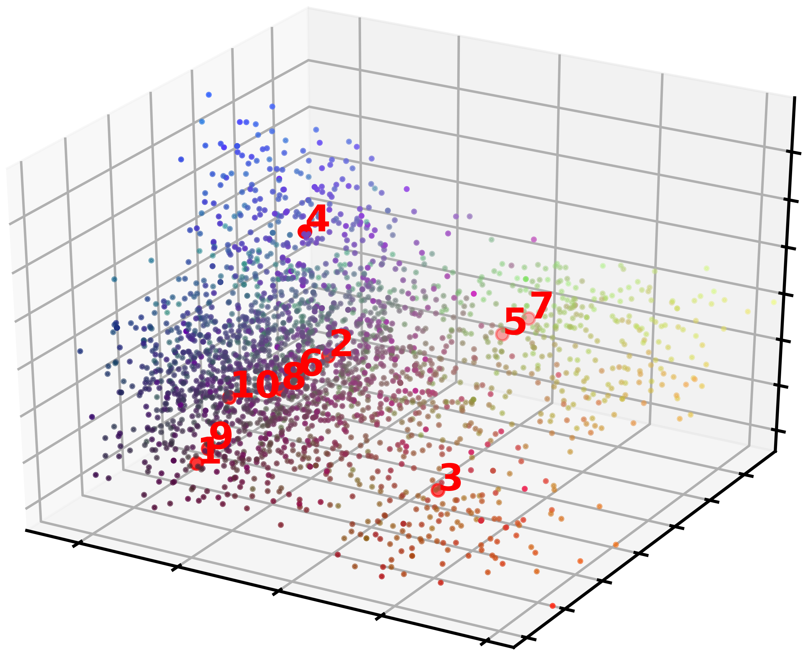
To give a concrete sense of the topics identified with ProSiT, in Table 6 we list the descriptors identified for Tweet with $\alpha=0.0001,\beta=0.2$ and SBERT representations as input. The associated performance in Table 5, first column, 10-topics is $C_{V}=0.5909$ . Figure 3 shows the same topics with the text data points. Their dimensionality was reduced with truncated Singular Value Decomposition (SVD) Halko et al. (2011).

5 Discussion

According to various metrics, the results show that ProSiT can extract from corpora latent topics comparable to or even better than several standard and state-of-the-art models.

Google News is the only data set for which ProSiT does not exceed the other methods. The most effective models are agglomerative clustering and K-means, which outperform not only ProSiT but also neural-ProdLDA, LDA, and the CTMs (even though, in the last two cases, the models take different inputs).

This dominance of clustering methods is indicative. Agglomerative clustering follows a hierarchical procedure to separate the documents, minimizing the distance between data points; similarly, K-means minimizes the clusters’ inertia. Their objectives make these models most effective when the clusters are convex and isotropic. The results suggest that this is the case with Google News. Conversely, during the training iterations, ProSiT’s centroids have some freedom to move away from their original position. The centroid position is also affected by outliers, which makes ProSiT suitable for non-isotropic spaces; this explains ProSiT’s versatility on the other data sets. This intuition is confirmed by the IRBO values, where ProSiT outperforms the other models on Google News. This result indicates its ability to create diverse topics, incorporating peripheral data points more effectively in the clusters than agglomerative clustering and K-means.

ProSiT also offers vast possibilities for results interpretation. Since documents and topics are represented as points in the same vector space, the relation of each document with the topics can be expressed in terms of distance. Passing those distances to a SoftMax function Goodfellow et al. (2016), we obtain a probability distribution that describes the affinity of each document with each topic; this is similar to the $\theta$ distribution in LDA. Analogously, the IG gives the probability of each word belonging to the different topics. This distribution provides a value for every word in the vocabulary, not just the descriptors.

6 Related Work

This work proposes a possible solution to the drawbacks of the most common Topic Models algorithms. Aimed to overcome the necessity of guessing the topics’ number, Broderick et al. (2013) rely on a Bayesian non-parametric framework that generates priors for the topics’ identification. Similar goal characterizes the family of Spectral Topic Models Anandkumar et al. (2012); Arora et al. (2012); Mimno and Lee (2014); Lee et al. (2020). However, differently from ProSiT, they still rely on some stochastic process to obtain the topics’ distributions.

The success of deep learning methods in NLP has also fostered new methods in topic models. The most recent ones are the contextualized topic models (CTM), which have been proposed in two studies Bianchi et al. (2021b, a). They represent the first approach to incorporate the semantic knowledge of pre-trained language models like BERT Devlin et al. (2019) into topic models. Exploiting BERT’s multi-lingual models, CTMs can map documents from different languages in a unified space. CTMs build on the neural-ProdLDA Srivastava and Sutton (2017), a neural topic model based on variational autoencoders. These methods create latent document representations from which they reconstruct the documents’ words, approximating the Dirichlet prior with Gaussian distributions. ProSiT does not use Dirichlet priors. Also, CTMs and neural-ProdLDA require the number of topics as an input parameter, which we prefer to avoid as we believe this number should evolve from the data analysis. However, similarly to CTM, ProSiT can use pre-trained language model representations as input, with the subsequent possibility of building multi-lingual topic models.

Deep learning methods are also the base for Top2Vec by Angelov (2020). Similarly to ProSiT, this method identifies topics in the same vector space as the documents, aggregating them according to their similarity. However, the author determines the topics’ descriptors from the position of word embeddings, which have to lie in the same vector space. Conversely, ProSiT extracts the topic descriptors directly from the documents. This feature makes ProSiT more flexible concerning different document representations. Sia et al. (2020) proposed a clustering procedure that creates topics starting from word embeddings, which are re-ranked using document information. Their procedure performs well compared to an LDA baseline (which ProSiT also easily beats). Recently, Grootendorst (2022) has proposed BERTopic, an effective model that first clusters documents together using sentence embeddings and then selects the most relevant keywords using class-based TF-IDF. We leave the comparison of ProSiT and BERTopic for future work.

Gialampoukidis et al. (2016) propose a hybrid procedure, which relies on DBSCAN Ester et al. (1996) to determine the clusters, whose number is used as the number of topics to compute LDA. This procedure is an effective way to provide LDA with a qualified prior on the number of topics. Indeed, DBSCAN is a widely used method for topic models Schubert et al. (2017). Using the points’ density, it can determine an optimal number of topics. However, it is not entirely deterministic (it starts from random points, and the cluster boundaries can be identified in different ways). Also, DBSCAN discards outliers, which is not a desirable feature for topic models, where every document should be evaluated. Its computational efficiency was a subject of debate, with differing opinions among researchers Gan and Tao (2015); Schubert et al. (2017). ProSiT, in contrast, uses all documents. The previous literature focuses on well-known methods for topic models and clustering, such as LDA Blei et al. (2003) and K-means Sculley (2010). Our method is more similar to the latter, as it derives topics elaborating from the original position of the documents in the vector space.

7 Conclusions

Latent topic models are crucial tools for data exploration. However, in many scientific fields, such as the social sciences, and many application areas, such as legal contexts, the theoretical motivation of the analyses is as essential as the quality of their outcome. The random initialization and necessary a priori decision of the number of topics are particularly weak motivations and can invalidate even high-quality topics unusable for those areas. ProSiT provides a viable answer to the need for interpretable high-quality topic models that are data driven rather than imposed a priori. ProSiT’s outcomes are transparent: they reflect the degrees of similarity explored to cluster the documents (for the topics’ identification) and the degrees of proximity between documents and topics (for the topic descriptors’ extraction). This is preferable to guess directly the topics’ number, as the outcomes lie on a meaningful continuum, rather than resulting from a (random) guess

ProSiT’s performance is comparable or higher than that of several other state-of-the-art methods. ProSiT’s setup allows users to explore several texts’ representations, from dense embeddings to sparse feature vectors.

Ethical considerations

ProSiT is a method to cluster documents according to their latent similarity; we do not consider this procedure harmful per se. However, as the input documents and their representations can carry unwanted biases, unethical content, and personal information, this could be reflected in ProSiT’s outcomes. Therefore, we invite a careful and responsible use of this method.

References

Anandkumar et al. (2012) Animashree Anandkumar, Daniel Hsu, and Sham M Kakade. 2012. A method of moments for mixture models and hidden markov models. In Conference on Learning Theory, pages 33–1. JMLR Workshop and Conference Proceedings.
Angelov (2020) Dimo Angelov. 2020. Top2vec: Distributed representations of topics. arXiv e-prints, pages arXiv–2008.
Arora et al. (2012) Sanjeev Arora, Rong Ge, and Ankur Moitra. 2012. Learning topic models–going beyond svd. In 2012 IEEE 53rd annual symposium on foundations of computer science, pages 1–10. IEEE.
Bianchi et al. (2021a) Federico Bianchi, Silvia Terragni, and Dirk Hovy. 2021a. Pre-training is a hot topic: Contextualized document embeddings improve topic coherence. In Proceedings of the 59th Annual Meeting of the Association for Computational Linguistics and the 11th International Joint Conference on Natural Language Processing (Volume 2: Short Papers), pages 759–766, Online. Association for Computational Linguistics.
Bianchi et al. (2021b) Federico Bianchi, Silvia Terragni, Dirk Hovy, Debora Nozza, and Elisabetta Fersini. 2021b. Cross-lingual contextualized topic models with zero-shot learning. In Proceedings of the 16th Conference of the European Chapter of the Association for Computational Linguistics: Main Volume, pages 1676–1683, Online. Association for Computational Linguistics.
Blei et al. (2003) David M Blei, Andrew Y Ng, and Michael I Jordan. 2003. Latent dirichlet allocation. the Journal of machine Learning research, 3:993–1022.
Broderick et al. (2013) Tamara Broderick, Brian Kulis, and Michael Jordan. 2013. Mad-bayes: Map-based asymptotic derivations from bayes. In International Conference on Machine Learning, pages 226–234. PMLR.
Burrough et al. (2015) Peter A Burrough, Rachael McDonnell, Rachael A McDonnell, and Christopher D Lloyd. 2015. Principles of geographical information systems. Oxford university press.
Devlin et al. (2019) Jacob Devlin, Ming-Wei Chang, Kenton Lee, and Kristina Toutanova. 2019. BERT: Pre-training of deep bidirectional transformers for language understanding. In Proceedings of the 2019 Conference of the North American Chapter of the Association for Computational Linguistics: Human Language Technologies, Volume 1 (Long and Short Papers), pages 4171–4186, Minneapolis, Minnesota. Association for Computational Linguistics.
Ding et al. (2018) Ran Ding, Ramesh Nallapati, and Bing Xiang. 2018. Coherence-aware neural topic modeling. In Proceedings of the 2018 Conference on Empirical Methods in Natural Language Processing, pages 830–836.
Ester et al. (1996) Martin Ester, Hans-Peter Kriegel, Jörg Sander, Xiaowei Xu, et al. 1996. A density-based algorithm for discovering clusters in large spatial databases with noise. In Kdd, volume 96, pages 226–231.
Ethayarajh (2019) Kawin Ethayarajh. 2019. How contextual are contextualized word representations? comparing the geometry of BERT, ELMo, and GPT-2 embeddings. In Proceedings of the 2019 Conference on Empirical Methods in Natural Language Processing and the 9th International Joint Conference on Natural Language Processing (EMNLP-IJCNLP), pages 55–65, Hong Kong, China. Association for Computational Linguistics.
Forman et al. (2003) George Forman et al. 2003. An extensive empirical study of feature selection metrics for text classification. J. Mach. Learn. Res., 3(Mar):1289–1305.
Gan and Tao (2015) Junhao Gan and Yufei Tao. 2015. Dbscan revisited: mis-claim, un-fixability, and approximation. In Proceedings of the 2015 ACM SIGMOD international conference on management of data, pages 519–530.
Gialampoukidis et al. (2016) Ilias Gialampoukidis, Stefanos Vrochidis, and Ioannis Kompatsiaris. 2016. A hybrid framework for news clustering based on the dbscan-martingale and lda. In International Conference on Machine Learning and Data Mining in Pattern Recognition, pages 170–184. Springer.
Goodfellow et al. (2016) Ian Goodfellow, Yoshua Bengio, Aaron Courville, and Yoshua Bengio. 2016. Deep learning, volume 1. MIT press Cambridge.
Grootendorst (2022) Maarten Grootendorst. 2022. Bertopic: Neural topic modeling with a class-based tf-idf procedure. arXiv preprint arXiv:2203.05794.
Halko et al. (2011) Nathan Halko, Per-Gunnar Martinsson, and Joel A Tropp. 2011. Finding structure with randomness: Probabilistic algorithms for constructing approximate matrix decompositions. SIAM review, 53(2):217–288.
Kullback and Leibler (1951) S. Kullback and R. A. Leibler. 1951. On information and sufficiency. Ann. Math. Statist., 22(1):79–86.
Lee et al. (2020) Moontae Lee, David Bindel, and David Mimno. 2020. Prior-aware composition inference for spectral topic models. In International Conference on Artificial Intelligence and Statistics, pages 4258–4268. PMLR.
Maimon and Rokach (2010) Oded Maimon and Lior Rokach. 2010. Data Mining and Knowledge Discovery Handbook, volume 14. Springer Science & Business Media.
Mikolov et al. (2013) Tomas Mikolov, Ilya Sutskever, Kai Chen, Greg S Corrado, and Jeff Dean. 2013. Distributed representations of words and phrases and their compositionality. Advances in Neural Information Processing Systems, 26:3111–3119.
Mimno and Lee (2014) David Mimno and Moontae Lee. 2014. Low-dimensional embeddings for interpretable anchor-based topic inference. In Proceedings of the 2014 Conference on Empirical Methods in Natural Language Processing (EMNLP), pages 1319–1328.
Qiang et al. (2020) Jipeng Qiang, Zhenyu Qian, Yun Li, Yunhao Yuan, and Xindong Wu. 2020. Short text topic modeling techniques, applications, and performance: a survey. IEEE Transactions on Knowledge and Data Engineering.
Reimers and Gurevych (2019) Nils Reimers and Iryna Gurevych. 2019. Sentence-bert: Sentence embeddings using siamese bert-networks. In Proceedings of the 2019 Conference on Empirical Methods in Natural Language Processing and the 9th International Joint Conference on Natural Language Processing (EMNLP-IJCNLP), pages 3973–3983.
Röder et al. (2015) Michael Röder, Andreas Both, and Alexander Hinneburg. 2015. Exploring the space of topic coherence measures. In Proceedings of the eighth ACM international conference on Web search and data mining, pages 399–408.
Rogers et al. (2020) Anna Rogers, Olga Kovaleva, and Anna Rumshisky. 2020. A primer in BERTology: What we know about how BERT works. Transactions of the Association for Computational Linguistics, 8:842–866.
Schubert et al. (2017) Erich Schubert, Jörg Sander, Martin Ester, Hans Peter Kriegel, and Xiaowei Xu. 2017. Dbscan revisited, revisited: why and how you should (still) use dbscan. ACM Transactions on Database Systems (TODS), 42(3):1–21.
Sculley (2010) David Sculley. 2010. Web-scale k-means clustering. In Proceedings of the 19th international conference on World wide web, pages 1177–1178.
Sia et al. (2020) Suzanna Sia, Ayush Dalmia, and Sabrina J. Mielke. 2020. Tired of topic models? clusters of pretrained word embeddings make for fast and good topics too! In Proceedings of the 2020 Conference on Empirical Methods in Natural Language Processing (EMNLP), pages 1728–1736, Online. Association for Computational Linguistics.
Srivastava and Sutton (2017) Akash Srivastava and Charles Sutton. 2017. Autoencoding variational inference for topic models. arXiv preprint arXiv:1703.01488.
Webber et al. (2010) William Webber, Alistair Moffat, and Justin Zobel. 2010. A similarity measure for indefinite rankings. ACM Transactions on Information Systems (TOIS), 28(4):1–38.

Appendix A Appendix

A.1 NPMI values

Input	SBERT embeddings			BoW
Topics	ProSiT	CTM	ZSTM	ProSiT	Agg.	Agg.+KM	KM	N-PLDA	LDA	DBScan
5	0.1749*	0.0672	0.0577	0.1832*	0.0799	0.0713	0.0741	0.0363	0.074
6		0.0667*	0.0588	0.2124*	0.0889	0.1071	0.0755	0.0215	0.0686
7	0.1653*	0.0853	0.104		0.0826	0.0907	0.0902	0.1056*	0.069
8		0.1405*	0.125	0.1416*	0.1112	0.1103	0.0888	0.1225	0.0581
9	0.113	0.1463*	0.1381	0.142	0.1057	0.1055	0.1098	0.1494*	0.0581
10		0.1652	0.2032*		0.0972	0.1041	0.0795	0.1593*	0.0599
11	0.0801	0.1649*	0.1343		0.0895	0.0963	0.0748	0.1463*	0.0556
13	0.1399	0.1285	0.1424*	0.1313	0.09	0.0881	0.0952	0.1454*	0.0672
15		0.1557	0.1613*	0.1267	0.0926	0.0951	0.0895	0.1318*	0.0767
16		0.1483	0.1533*	0.1349	0.0882	0.09	0.0887	0.1456*	0.0719
17	0.1068	0.1511*	0.1275		0.096	0.0992	0.0922	0.1473*	0.0731
20		0.1395	0.141*		0.0848	0.0913	0.0905	0.133*	0.0753	-0.0329
21	0.1131	0.1346	0.1494*		0.096	0.0995	0.1006	0.1351*	0.0681
25		0.1532*	0.1458		0.096	0.0988	0.1161	0.1637*	0.0791

Table 7: NPMI values for Reuters data set.

Input	SBERT embeddings			BoW
Topics	ProSiT	CTM	ZSTM	ProSiT	Agg.	Agg.+KM	KM	N-PLDA	LDA	DBScan
5		0.1947	0.2058*	0.1793	0.2975*	0.2975	0.2975	0.1364	0.076
6	0.1247	0.1453	0.1989*	0.2098	0.285*	0.285	0.285	0.1822	0.0674
7	0.1455	0.0811	0.2076*		0.2956*	0.2956	0.2956	0.1489	0.0798
10		0.1317	0.1806*		0.2768	0.2813	0.286*	0.1101	0.0699
11		0.1021	0.1189*	0.1195	0.2837*	0.2829	0.2832	0.0784	0.0712
12	0.1761*	0.1052	0.1285		0.3012*	0.3004	0.2605	0.1306	0.0668
13	0.1468	0.1297	0.158*	0.1779	0.2958	0.2967*	0.2919	0.1444	0.1048
15		0.1529	0.1677*		0.2973	0.2981	0.3051*	0.1186	0.0958
20	0.0836	0.1095	0.1605*		0.252	0.2516	0.2777*	0.0814	0.0759
22	0.0978	0.0971	0.1393*	0.1335	0.2448	0.2444	0.2615*	0.1301	0.0769
25		0.1102*	0.1034	0.123	0.2458	0.2456	0.2611*	0.0629	0.0938

Table 8: NPMI values for Google News data set.

Input	SBERT embeddings			BoW
Topics	ProSiT	CTM	ZSTM	ProSiT	Agg.	Agg.+KM	KM	N-PLDA	LDA	DBScan
5		0.0148*	0.005	0.204*	0.1364	0.1447	0.1129	0.02	0.087
8	0.2003*	0.1125	0.1282	0.2227*	0.1661	0.1743	0.1282	0.1151	0.071
10		0.133	0.1472*		0.1867*	0.1827	0.1612	0.1762	0.0751
13	0.2218*	0.1419	0.1656	0.2052*	0.1854	0.1762	0.177	0.1328	0.0833
15	0.1913*	0.1592	0.1687		0.1766	0.1661	0.1751	0.1874*	0.0784
18		0.1809*	0.1781		0.1772	0.1677	0.1804*	0.1602	0.0795	0.066
20		0.1633	0.1783*		0.1805	0.1704	0.1449	0.1945*	0.0992
23	0.1917	0.1862	0.2054*	0.2004*	0.1846	0.179	0.1609	0.1787	0.1026
24		0.1861	0.1954*	0.2159*	0.1861	0.1817	0.1602	0.1897	0.1124
25	0.1984*	0.1938	0.1829		0.1853	0.1809	0.1495	0.2008*	0.1019

Table 9: NPMI values for Wiki20K data set.

Input	SBERT embeddings			BoW
Topics	ProSiT	CTM	ZSTM	ProSiT	Agg.	Agg.+KM	KM	N-PLDA	LDA	DBScan
5		-0.2336	-0.1261*		0.1733	0.1734*	0.1366	-0.2384	-0.3048
6		-0.2005	-0.145*	0.3094*	0.112	0.1256	0.1632	-0.2621	-0.191
10	0.1784*	-0.0997	-0.0981		0.191	0.1916*	0.1786	-0.0612	-0.23
11		-0.1069	-0.0259*	0.1144	0.1865	0.1804	0.2092*	-0.1405	-0.213
15		-0.0266	0.0219*		0.2145	0.2175*	0.1929	-0.0406	-0.191
19	0.1522*	0.0115	0.0006		0.2161	0.2217*	0.2211	-0.0713	-0.1456
20		0.0331	0.0578*		0.2263	0.2333	0.2592*	0.0421	-0.1677
23		0.0429*	0.028		0.2507	0.2546*	0.2437	0.0442	-0.1689	0.0543
25		0.0331*	0.0078		0.2602	0.2622*	0.2572	0.0998	-0.1571

Table 10: NPMI values for Tweet data set.

A.2 IRBO values

Input	SBERT embeddings			BoW
Topics	ProSiT	CTM	ZSTM	ProSiT	Agg.	Agg.+KM	KM	N-PLDA	LDA	DBScan
5	0.9566	1.0*	1.0	1.0*	0.6242	0.6681	0.6743	1.0*	0.7094
6		0.9852	0.9974*	0.9912	0.6598	0.6673	0.5855	1.0*	0.727
7	0.9757	0.9899	0.9927*		0.6683	0.6433	0.6386	1.0*	0.7406
8		0.9873	0.9968*	1.0*	0.6756	0.6485	0.6474	0.9942	0.7385
9	0.9931*	0.9785	0.984	1.0*	0.7008	0.6697	0.6444	0.9903	0.7589
10		0.9796	0.9869*		0.6967	0.6656	0.6532	0.9816*	0.7588
11	0.9856*	0.9832	0.9814		0.6912	0.6736	0.6433	0.9779*	0.7488
13	0.9948*	0.9808	0.987	0.9846	0.7042	0.6911	0.6909	0.9847*	0.7689
15		0.9805	0.9807*	0.9889*	0.7367	0.7284	0.7168	0.9825	0.7683
16		0.9758*	0.9738	0.9883*	0.742	0.7207	0.7024	0.984	0.7865
17	0.995*	0.9786	0.9767		0.7424	0.7271	0.7146	0.9782*	0.7733
20		0.975	0.979*		0.7337	0.7294	0.7155	0.9797*	0.7981	0.9244
21	0.9971*	0.9719	0.9782		0.7353	0.7419	0.732	0.9793*	0.7801
25		0.9749	0.9803*		0.7414	0.7502	0.7643	0.9825*	0.8099

Table 11: IRBO values for Reuters data set.

Input	SBERT embeddings			BoW
Topics	ProSiT	CTM	ZSTM	ProSiT	Agg.	Agg.+KM	KM	N-PLDA	LDA	DBScan
5		0.9591	0.977*	1.0*	0.551	0.551	0.551	0.984	0.8398
6	1.0*	0.9904	0.9776	1.0*	0.4982	0.4982	0.4982	0.9715	0.908
7	1.0*	0.9583	0.9908		0.4886	0.4886	0.4886	0.9823*	0.8773
10		0.9728*	0.9592		0.6516	0.6526	0.6569	0.9656*	0.9244
11		0.9646	0.9773*	1.0*	0.7111	0.7105	0.7101	0.9806	0.9313
12	1.0*	0.9759	0.9644		0.7579	0.7574	0.6799	0.9829*	0.9232
13	1.0*	0.9387	0.974	1.0*	0.7947	0.7943	0.7905	0.9758	0.9255
15		0.9641	0.9909*		0.743	0.7427	0.7436	0.9819*	0.9372
20	0.9994*	0.9835	0.9757		0.8455	0.8448	0.8452	0.9874*	0.9415
22	0.9996*	0.9844	0.9881	0.994*	0.8712	0.8705	0.8525	0.981	0.9404
25		0.9872*	0.9867	0.9969*	0.8819	0.8813	0.8783	0.9781	0.9488

Table 12: IRBO values for Google News data set.

Input	SBERT embeddings			BoW
Topics	ProSiT	CTM	ZSTM	ProSiT	Agg.	Agg.+KM	KM	N-PLDA	LDA	DBScan
5	1.0*	1.0*	1.0	0.942	0.9371	0.9429	0.9309	1.0*	0.9511
8	1.0*	0.9986	1.0	0.9897	0.9523	0.9532	0.9359	1.0*	0.9503
10		1.0*	0.9987		0.9535	0.9543	0.9431	0.9991*	0.9469
13	1.0*	0.9985	0.9987	0.995	0.9481	0.9412	0.9395	0.9994*	0.9594
15	1.0*	0.9992	0.9985		0.949	0.9392	0.9482	0.9995*	0.9618
18		0.9991*	0.9975		0.9436	0.9424	0.9516	0.999*	0.968	0.9293
20		0.9984*	0.9977		0.9503	0.9458	0.9277	0.9974*	0.9722
23	1.0*	0.9968	0.9981	0.9961	0.9537	0.948	0.9412	0.9982*	0.9725
24		0.9967	0.9983*	0.9958	0.9555	0.9499	0.9492	0.9978*	0.976
25	1.0*	0.997	0.9979		0.9543	0.9493	0.9482	0.9979*	0.9801

Table 13: IRBO values for Wiki20K data set.

Input	SBERT embeddings			BoW
Topics	ProSiT	CTM	ZSTM	ProSiT	Agg.	Agg.+KM	KM	N-PLDA	LDA	DBScan
5		1.0*	1.0	1.0*	0.9796	0.9796	0.9943	1.0*	0.9176
6		1.0*	1.0	1.0*	0.9864	0.9835	0.9838	1.0	0.9283
10	0.9943	1.0*	1.0		0.9845	0.9819	0.9808	1.0*	0.9332
11		1.0*	1.0	0.9985	0.9866	0.9844	0.9814	0.9993*	0.9575
15		0.9992*	0.9985		0.9912	0.9893	0.9756	1.0*	0.9516
19	0.9988*	0.9939	0.9962		0.9896	0.9899	0.9828	0.9989*	0.9671
20		0.9975	0.9977*		0.9906	0.9909	0.9836	0.9988*	0.9687
23		0.9957	0.9975*		0.9926	0.9925	0.986	0.9963*	0.9724	0.9075
25		0.9912	0.9955*		0.9932	0.9929	0.9799	0.9977*	0.9718

Table 14: IRBO for Tweet data set.

A.3 WECO values

Input	SBERT embeddings			BoW
Topics	ProSiT	CTM	ZSTM	ProSiT	Agg.	Agg.+KM	KM	N-PLDA	LDA	DBScan
5	0.2174*	0.1701	0.163	0.2217*	0.183	0.1661	0.1612	0.1701	0.1801
6		0.153	0.1888*	0.1824	0.1861*	0.1821	0.1842	0.1667	0.183
7	0.2122*	0.17	0.1757		0.1805*	0.1793	0.1793	0.175	0.1763
8		0.1895*	0.1873	0.1823	0.1876*	0.1831	0.1699	0.181	0.17
9	0.1963	0.2017*	0.1804	0.1931*	0.189	0.1812	0.1801	0.1848	0.1721
10		0.1845	0.2045*		0.1844*	0.1736	0.17	0.1766	0.1685
11	0.2082*	0.1913	0.185		0.1829	0.1818	0.1764	0.1864*	0.1653
13	0.1933*	0.1853	0.1843	0.1692	0.1785	0.1811	0.1793	0.1852*	0.1694
15		0.185	0.1959*	0.1715	0.1766*	0.1753	0.1748	0.1752	0.1653
16		0.1821*	0.1758	0.1854	0.1744	0.1751	0.1772	0.192*	0.1666
17	0.1708	0.1809*	0.1782		0.1745	0.1739	0.1818*	0.1691	0.1695
20		0.1659	0.1676*		0.1747	0.1708	0.1724	0.1763*	0.1572	0.0973
21	0.1595	0.1707*	0.1705		0.1768	0.1739	0.179*	0.1691	0.1563
25		0.1667	0.1779*		0.175*	0.1708	0.1719	0.1655	0.148

Table 15: WECO values for Reuters data set.

Input	SBERT embeddings			BoW
Topics	ProSiT	CTM	ZSTM	ProSiT	Agg.	Agg.+KM	KM	N-PLDA	LDA	DBScan
5		0.2257	0.2582*	0.2527	0.2622*	0.2622	0.2622	0.2616	0.2239
6	0.2145	0.22	0.2612*	0.2273	0.2611*	0.2611	0.2611	0.2366	0.216
7	0.2162*	0.1919	0.2149		0.2504*	0.2504	0.2504	0.2235	0.1978
10		0.2169	0.2329*		0.2338*	0.2338	0.2309	0.2164	0.1898
11		0.2104*	0.2059	0.1966	0.2244	0.2259	0.2268*	0.1927	0.1996
12	0.2093	0.2015	0.2179*		0.2373	0.2386*	0.2345	0.2311	0.2043
13	0.1935	0.2086	0.2277*	0.1966	0.2355	0.2369*	0.235	0.2185	0.1989
15		0.1965	0.2123*		0.2387	0.2398*	0.2317	0.1963	0.1906
20	0.1741	0.1815	0.1822*		0.226	0.226	0.2385*	0.2027	0.1905
22	0.1826	0.1886*	0.1876	0.1814	0.2204	0.2205*	0.2163	0.2003	0.1843
25		0.1918	0.2008*	0.1916	0.2135	0.2137	0.2199*	0.1772	0.1799

Table 16: WECO values for Google News data set.

Input	SBERT embeddings			BoW
Topics	ProSiT	CTM	ZSTM	ProSiT	Agg.	Agg.+KM	KM	N-PLDA	LDA	DBScan
5		0.2015	0.2125*	0.1864	0.257	0.2608*	0.2258	0.2239	0.1946
8	0.2138	0.1952	0.2184*	0.1748	0.2246	0.2315*	0.2249	0.2019	0.1673
10		0.2081	0.2155*		0.2184*	0.2101	0.2039	0.2105	0.1701
13	0.2474*	0.2172	0.2074	0.1695	0.2135*	0.2122	0.208	0.1999	0.1706
15	0.2111	0.2071	0.2204*		0.2074	0.2006	0.207	0.2135*	0.1745
18		0.208	0.2232*		0.2027	0.1983	0.1929	0.2239*	0.1612	0.1234
20		0.1938	0.2095*		0.1994	0.2032*	0.1967	0.2032	0.1701
23	0.2054	0.2136	0.2149*	0.1766	0.2056	0.2077	0.2126*	0.2033	0.164
24		0.1981	0.2192*	0.1709	0.2026	0.2042	0.1922	0.2053*	0.1737
25	0.1993	0.1965	0.2186*		0.2053	0.2091*	0.1979	0.2074	0.1668

Table 17: WECO values for Wiki20K data set.

Input	SBERT embeddings			BoW
Topics	ProSiT	CTM	ZSTM	ProSiT	Agg.	Agg.+KM	KM	N-PLDA	LDA	DBScan
5		0.1287*	0.1226		0.1445	0.1471*	0.143	0.1242	0.1066
6		0.1498*	0.1175	0.1315	0.1434	0.1499*	0.1498	0.1267	0.1124
10	0.1619*	0.1475	0.1458		0.1473	0.1574*	0.1562	0.1388	0.1168
11		0.1612*	0.147	0.1278	0.1619	0.1712*	0.1348	0.1374	0.121
15		0.1599*	0.156		0.1531	0.1602*	0.1441	0.143	0.1109
19	0.138	0.1521	0.1522*		0.1515	0.1572*	0.1533	0.1405	0.1049
20		0.1487	0.1577*		0.1523	0.1573*	0.1553	0.1386	0.114
23		0.1563	0.1617*		0.1578	0.1623*	0.1574	0.1509	0.1208	0.1034
25		0.1472	0.1511*		0.157	0.1614*	0.1553	0.1452	0.1121

Table 18: WECO values for Tweet data set.

A.4 Specificity values

Input	SBERT embeddings			BoW
Topics	ProSiT	CTM	ZSTM	ProSiT	Agg.	Agg.+KM	KM	N-PLDA	LDA	DBScan
5	1.4708	1.6094*	1.6094	1.443	0.8017	0.873	0.8835	1.6094*	1.0062
6		1.7224	1.7686*	1.7224	0.9095	0.914	0.767	1.7917*	1.0947
7	1.7874	1.8666	1.8864*		1.0166	0.9065	0.8788	1.9458*	1.2851
8		1.9581	2.0447*	2.0794*	1.0179	0.904	0.9491	2.0274	1.35
9	2.1201*	2.0123	2.0585	2.1971*	1.1531	1.0179	0.9222	2.1047	1.5212
10		2.1084	2.1777*		1.2001	1.0347	1.0897	2.1223*	1.5763
11	2.237*	2.234	2.234		1.2194	1.1312	1.1036	2.1866*	1.4958
13	2.4918*	2.3862	2.4155	2.3918	1.2885	1.1686	1.2379	2.4115*	1.6679
15		2.4525	2.4872*	2.5641*	1.4459	1.342	1.3702	2.4884	1.7475
16		2.469*	2.4653	2.6093*	1.4773	1.3603	1.3751	2.5547	1.9032
17	2.7597*	2.5537	2.5823		1.4562	1.3921	1.3508	2.5537*	1.8883
20		2.635	2.7052*		1.5268	1.5015	1.4407	2.7248*	1.989	2.1794
21	2.9783*	2.6428	2.7447		1.5273	1.5209	1.5019	2.7364*	2.0082
25		2.8436	2.8942*		1.6526	1.6331	1.6837	2.9399*	2.2226

Table 19: Specificity values for Reuters data set.

Input	SBERT embeddings			BoW
Topics	ProSiT	CTM	ZSTM	ProSiT	Agg.	Agg.+KM	KM	N-PLDA	LDA	DBScan
5		1.4326	1.4985*	1.6094*	0.8331	0.8331	0.8331	1.5262	1.2071
6	1.7917*	1.7224	1.6531	1.7917*	0.8726	0.8726	0.8726	1.63	1.4739
7	1.9458*	1.7676	1.8666		0.9169	0.9169	0.9169	1.8468*	1.5075
10		2.1118*	2.0043		1.2688	1.2827	1.3104	2.0702*	1.9318
11		2.1567	2.2228*	2.3978*	1.4329	1.4203	1.4203	2.2922	2.0403
12	2.4848*	2.3187	2.2045		1.5772	1.5656	1.3979	2.3534*	2.0444
13	2.5648*	2.1589	2.3208	2.5648*	1.7164	1.7057	1.691	2.3689	2.0941
15		2.3705	2.6028*		1.6717	1.6625	1.6959	2.5403*	2.2098
20	2.9828*	2.7728	2.7231		2.0667	2.0624	2.0676	2.8491*	2.4686
22	3.0785*	2.8529	2.9199	2.9893*	2.2212	2.211	2.1862	2.8671	2.5818
25		2.9698	3.0007*	3.1465*	2.3682	2.3537	2.3135	3.0356	2.6802

Table 20: Specificity values for Google News data set.

Input	SBERT embeddings			BoW
Topics	ProSiT	CTM	ZSTM	ProSiT	Agg.	Agg.+KM	KM	N-PLDA	LDA	DBScan
5		1.6094*	1.6094	1.443	1.3321	1.3599	1.2662	1.6094*	1.4049
8	2.0794*	2.062	2.0794	2.01	1.7544	1.7652	1.6547	2.0794*	1.7685
10		2.3025*	2.2886		1.935	1.9325	1.8388	2.2886*	1.9507
13	2.5648*	2.5435	2.5435	2.5008	2.0675	2.0047	2.0144	2.5542*	2.1643
15	2.7079*	2.6894	2.6894		2.1729	2.0862	2.2128	2.6987*	2.293
18		2.8748*	2.8671		2.2281	2.2029	2.3116	2.8748*	2.4555	2.0711
20		2.9539	2.9609*		2.3723	2.3081	2.1905	2.947*	2.6156
23	3.1353*	3.0486	3.087	3.0538	2.4895	2.4021	2.3161	3.0931*	2.7141
24		3.097	3.1201*	3.1006	2.5302	2.4398	2.4627	3.1258*	2.7608
25	3.2186*	3.1389	3.1632		2.5498	2.4629	2.4282	3.1666*	2.845

Table 21: Specificity values for Wiki20K data set.

Input	SBERT embeddings			BoW
Topics	ProSiT	CTM	ZSTM	ProSiT	Agg.	Agg.+KM	KM	N-PLDA	LDA	DBScan
5		1.6094*	1.6094		1.5262	1.5262	1.5817	1.6094*	1.3494
6		1.7917*	1.7917	1.7999*	1.7224	1.6993	1.6993	1.7917	1.4826
10	2.2332	2.3025*	2.3025		2.162	2.1257	2.1777	2.3025*	1.85
11		2.3978*	2.3978	2.3726	2.2575	2.2244	2.2401	2.3852*	2.1087
15		2.6894*	2.6802		2.59	2.5566	2.4594	2.7079*	2.3294
19	2.9304*	2.8612	2.8786		2.7828	2.781	2.6879	2.9224*	2.583
20		2.9539*	2.947		2.8421	2.8404	2.7451	2.9747*	2.6354
23		3.0569	3.069*		2.9898	2.9763	2.8949	3.0569*	2.772	1.9899
25		3.0682	3.1355*		3.0703	3.0523	2.8883	3.1632*	2.818

Table 22: Specificity values for Tweet data set.

A.5 Dissimilarity values

Input	SBERT embeddings			BoW
Topics	ProSiT	CTM	ZSTM	ProSiT	Agg.	Agg.+KM	KM	N-PLDA	LDA	DBScan
5	0.3657*	0.3536	0.3536	0.3657*	0.364	0.3317	0.3202	0.3536	0.3518
6		0.3499*	0.3476	0.3533*	0.3262	0.3187	0.3237	0.3464	0.3441
7	0.3512*	0.3448	0.344		0.3215	0.3153	0.3091	0.3416*	0.3391
8		0.3423*	0.3393	0.3381	0.3307	0.3175	0.3117	0.3399*	0.3387
9	0.3387	0.341*	0.3396	0.3354	0.3298	0.3062	0.3092	0.3382*	0.3345
10		0.3385*	0.3367		0.3304	0.301	0.3243	0.3381*	0.3239
11	0.3362*	0.3356	0.3356		0.3219	0.298	0.3197	0.337*	0.3292
13	0.3676*	0.3329	0.3321	0.4142*	0.3219	0.2995	0.3175	0.3323	0.3389
15		0.3323*	0.3315	0.3898*	0.3403	0.3429	0.3314	0.3315	0.3327
16		0.3323	0.3325*	0.3606*	0.3372	0.3415	0.3094	0.3303	0.3286
17	0.331*	0.3307	0.3302		0.34	0.3418*	0.3321	0.3305	0.324
20		0.3299*	0.3288		0.3344	0.3362	0.3371	0.3284	0.3395*	0.338
21	0.3249	0.33*	0.3283		0.3358	0.336	0.3375	0.3284	0.34*
25		0.3273*	0.3265		0.3314	0.3301	0.3411*	0.3262	0.3377

Table 23: Dissimilarity values for Reuters data set.

Input	SBERT embeddings			BoW
Topics	ProSiT	CTM	ZSTM	ProSiT	Agg.	Agg.+KM	KM	N-PLDA	LDA	DBScan
5		0.3657*	0.3606	0.3588	0.4153*	0.4153	0.4153	0.3588	0.3824
6	0.3499	0.3499	0.3533*	0.3464	0.4118*	0.4118	0.4118	0.3544	0.3655
7	0.3432	0.3488*	0.3448		0.4062*	0.4062	0.4062	0.3456	0.3651
10		0.3388	0.3435*		0.3794*	0.3791	0.3784	0.3399	0.3475
11		0.3379*	0.3367	0.3329	0.3701	0.3704*	0.3704	0.3344	0.3441
12	0.3303	0.335	0.3377*		0.3602	0.3604	0.3693*	0.3333	0.3447
13	0.3291	0.3399*	0.335	0.3291	0.3545	0.3547	0.3551*	0.3331	0.344
15		0.3349*	0.3292		0.3589	0.359*	0.3564	0.3304	0.3403
20	0.3611*	0.3275	0.3289		0.3424	0.3426*	0.3424	0.3266	0.3366
22	0.3846*	0.3265	0.3258	0.5738*	0.3386	0.3388	0.3408	0.3267	0.3348
25		0.3253*	0.3253	0.3793*	0.339	0.3392	0.3358	0.3251	0.3324

Table 24: Dissimilarity values for Google News data set.

Input	SBERT embeddings			BoW
Topics	ProSiT	CTM	ZSTM	ProSiT	Agg.	Agg.+KM	KM	N-PLDA	LDA	DBScan
5		0.3536*	0.3536	0.364*	0.3446	0.3518	0.341	0.3536	0.3588
8	0.3381	0.3387*	0.3381	0.3423	0.332	0.332	0.335	0.3381	0.3429*
10		0.3333	0.3337*		0.341	0.3385	0.3414*	0.3337	0.3341
13	0.3291	0.3296*	0.3296	0.3389	0.3391	0.3395*	0.3377	0.3294	0.3285
15	0.3273	0.3276*	0.3276		0.3375*	0.3372	0.3341	0.3275	0.3349
18		0.3256	0.3257*		0.3357*	0.3346	0.3293	0.3256	0.3261	0.3341
20		0.325*	0.3249		0.333	0.3327	0.3388*	0.325	0.3292
23	0.3235	0.3243*	0.3238	0.3251	0.3315	0.332	0.3322*	0.3238	0.3298
24		0.3238*	0.3236	0.3493*	0.3311	0.3316	0.3299	0.3236	0.3257
25	0.3227	0.3236*	0.3233		0.3311	0.3315*	0.3254	0.3233	0.3237

Table 25: Dissimilarity values for Wiki20K data set.

Input	SBERT embeddings			BoW
Topics	ProSiT	CTM	ZSTM	ProSiT	Agg.	Agg.+KM	KM	N-PLDA	LDA	DBScan
5		0.3536*	0.3536		0.3588*	0.3588	0.3553	0.3536	0.3536
6		0.3464*	0.3464	0.4036*	0.3499	0.351	0.351	0.3464	0.3555
10	0.3352*	0.3333	0.3333		0.3377	0.3385*	0.3367	0.3333	0.3344
11		0.3317*	0.3317	0.3323	0.3356	0.3362	0.3362	0.332	0.337*
15		0.3276	0.3278*		0.3298	0.3303	0.332*	0.3273	0.332
19	0.4105*	0.326	0.3257		0.3274	0.3273	0.3286*	0.3252	0.3263
20		0.325*	0.325		0.3267	0.3266	0.3277	0.3247	0.3289*
23		0.3242*	0.324		0.3251	0.3252	0.3263	0.3242	0.3288	0.3468*
25		0.3243*	0.3236		0.3245	0.3246	0.3267	0.3233	0.3289*

Table 26: Dissimilarity values for Tweet data set.

A.6 Comparison with Top2Vec and Sia et al. (2020) method

Input	Doc2Vec embeddings		Word2vec embeddings
	ProSiT	T2V	KM	Spherical-KM	GMM
5	0.7005*		0.356	0.3809	0.4485*
6			0.4154	0.4332*	0.431
7			0.4515	0.4702*	0.4492
8	0.7044*		0.4043	0.4361*	0.4333
9			0.405	0.4204*	0.3755
10			0.4187*	0.4186	0.3843
11			0.433*	0.4296	0.4102
13			0.4095	0.3794	0.4303*
15	0.6296*		0.4121	0.3772	0.4622*
16			0.4214	0.3966	0.4465*
17			0.3809	0.3964	0.45*
20			0.3931	0.3935	0.4418*
21			0.3905	0.4027	0.4353*
25	0.6744*		0.4063*	0.3661	0.4004
114		0.6546*

Table 27: Coherence values for Reuters data set.

Input	Doc2Vec embeddings		Word2vec embeddings
	ProSiT	T2V	KM	Spherical-KM	GMM
2		0.7799*
4	0.701*
5			0.4237*		0.391
6			0.3765	0.4836*	0.4322
7	0.711*		0.5109	0.5307*	0.4022
10			0.5008*	0.4967	0.4731
11			0.4748	0.491*	0.4734
12			0.5215*	0.5144	0.4736
13	0.7014*		0.4626	0.5006*	0.4934
15			0.5259	0.5363*	0.486
20	0.7022*		0.5654*	0.5385	0.5324
22			0.5052	0.5147	0.5297*
25			0.568*	0.5297	0.5286

Table 28: Coherence values for Google News data set.

Input	Doc2Vec embeddings		Word2vec embeddings
	ProSiT	T2V	KM	Spherical-KM	GMM
5	0.2013*		-0.2067	-0.0966*	-0.1316
6			-0.1502	-0.063*	-0.1563
7			-0.1527	-0.0542*	-0.1332
8	0.1981*		-0.1377	-0.0785*	-0.1056
9			-0.1395	-0.1011*	-0.1284
10			-0.1335	-0.1145*	-0.1312
11			-0.1345	-0.0869*	-0.1274
13			-0.1225	-0.1312	-0.0922*
15	0.1216*		-0.1384	-0.1345	-0.0925*
16			-0.113*	-0.1373	-0.113
17			-0.1565	-0.1219	-0.0966*
20			-0.137	-0.1445	-0.1016*
21			-0.1331	-0.132	-0.0874*
25	0.1777*		-0.124*	-0.152	-0.129
114		0.0994*

Table 29: NPMI values for Reuters data set.

Input	Doc2Vec embeddings		Word2vec embeddings
	ProSiT	T2V	KM	Spherical-KM	GMM
2		0.1873*
4	0.1466*
5			-0.153		-0.1215*
6			-0.13	-0.0747*	-0.0919
7	0.1595*		-0.0556	-0.0294*	-0.1073
10			-0.0705	-0.0626	-0.0424*
11			-0.0619	-0.035*	-0.0442
12			-0.0497	-0.0441	-0.0402*
13	0.1645*		-0.0519	-0.0389	-0.0268*
15			-0.0438	0.0091*	-0.0418
20	0.1514*		-0.011	-0.0156	-0.0087*
22			-0.0671	-0.0325	-0.0179*
25			-0.018	-0.0146*	-0.0204

Table 30: NPMI values for Google News data set.

Input	Doc2Vec embeddings		Word2vec embeddings
	ProSiT	T2V	KM	Spherical-KM	GMM
5	1.0*		1.0*	1.0	1.0
6			1.0*	1.0	1.0
7			1.0*	1.0	1.0
8	0.9955*		1.0*	1.0	1.0
9			1.0*	1.0	1.0
10			1.0*	1.0	1.0
11			1.0*	1.0	1.0
13			1.0*	1.0	1.0
15	0.9936*		1.0*	1.0	1.0
16			1.0*	1.0	1.0
17			1.0*	1.0	1.0
20			1.0*	1.0	1.0
21			1.0*	1.0	0.9998
25	0.9957*		1.0*	1.0	0.9999
114		0.9811*

Table 31: IRBO values for Reuters data set.

Input	Doc2Vec embeddings		Word2vec embeddings
	ProSiT	T2V	KM	Spherical-KM	GMM
2	1.0*	1.0*
4	1.0*
5			1.0*		1.0
6			1.0*	1.0	1.0
7	1.0*		1.0*	1.0	1.0
10			1.0*	1.0	1.0
11			1.0*	1.0	1.0
12			1.0*	1.0	1.0
13	1.0*		1.0*	1.0	1.0
15			1.0*	1.0	1.0
20	1.0*		1.0*	1.0	1.0
22			1.0*	1.0	0.9991
25			1.0*	1.0	0.9983

Table 32: IRBO values for Google News data set.

Input	Doc2Vec embeddings		Word2vec embeddings
	ProSiT	T2V	KM	Spherical-KM	GMM
5	0.1666*		0.2594	0.3847*	0.3187
6			0.2951	0.405*	0.3168
7			0.264	0.3975*	0.3514
8	0.2023*		0.3026	0.4196*	0.332
9			0.2755	0.3949*	0.3185
10			0.2815	0.3976*	0.3333
11			0.2951	0.3945*	0.3287
13			0.2764	0.3892*	0.3637
15	0.1735*		0.2844	0.3772	0.3902*
16			0.3211	0.3903*	0.3835
17			0.3017	0.3769	0.379*
20			0.3005	0.3689	0.3932*
21			0.2927	0.3811	0.3907*
25	0.1441*		0.3263	0.3641	0.3877*
114		0.164*

Table 33: WECO values for Reuters data set.

Input	Doc2Vec embeddings		Word2vec embeddings
	ProSiT	T2V	KM	Spherical-KM	GMM
2		0.3007*
4	0.2259*
5			0.237		0.2923*
6			0.2399	0.3808*	0.3096
7	0.2302*		0.2868	0.3622*	0.2968
10			0.2722	0.3525	0.3659*
11			0.2955	0.3418	0.3539*
12			0.283	0.3566	0.3653*
13	0.2412*		0.3054	0.3538	0.3697*
15			0.2863	0.3632*	0.3478
20	0.2054*		0.3276	0.3492*	0.341
22			0.2773	0.3447	0.3507*
25			0.3139	0.3198	0.3556*

Table 34: WECO values for Google News data set.

Input	Doc2Vec embeddings		Word2vec embeddings
	ProSiT	T2V	KM	Spherical-KM	GMM
5	1.6094*		1.6094*	1.6094	1.6094
6			1.7917*	1.7917	1.7917
7			1.9458*	1.9458	1.9458
8	2.0436*		2.0794*	2.0794	2.0794
9			2.1971*	2.1971	2.1971
10			2.3025*	2.3025	2.3025
11			2.3978*	2.3978	2.3978
13			2.4848	2.5648*	2.5648
15	2.6071*		2.6389	2.7079*	2.6389
16			2.7724*	2.7724	2.7079
17			2.7724*	2.7079	2.7724
20			2.9442	2.9442	2.9955*
21			3.0443*	2.9955	3.0377
25	3.1217*		3.2308*	3.1778	3.172
114		3.091*

Table 35: Specificity values for Reuters data set.

Input	Doc2Vec embeddings		Word2vec embeddings
	ProSiT	T2V	KM	Spherical-KM	GMM
2		0.6931*
4	1.3863*
5			1.6094*		1.6094
6			1.7917*	1.7917	1.7917
7	1.9458*		1.9458*	1.9458	1.9458
10			2.3025*	2.3025	2.3025
11			2.3025	2.3978*	2.3978
12			2.4848*	2.4848	2.4848
13	2.5648*		2.5648*	2.5648	2.5648
15			2.7082*	2.7079	2.7079
20	2.9955*		2.9955*	2.9442	2.9955
22			3.0908*	3.0908	3.0632
25			3.25*	3.2186	3.1666

Table 36: Specificity values for Google News data set.

Input	Doc2Vec embeddings		Word2vec embeddings
	ProSiT	T2V	KM	Spherical-KM	GMM
5	0.3536*		0.3536*	0.3536	0.3536
6			0.3464*	0.3464	0.3464
7			0.3416*	0.3416	0.3416
8	0.386*		0.3381*	0.3381	0.3381
9			0.3354*	0.3354	0.3354
10			0.3333*	0.3333	0.3333
11			0.3317*	0.3317	0.3317
13			0.3303*	0.3291	0.3291
15	0.4156*		0.3282*	0.3273	0.3282
16			0.3266	0.3266	0.3273*
17			0.3266	0.3273*	0.3266
20			0.3249*	0.3249	0.3244
21			0.324	0.3244*	0.3241
25	0.4442*		0.7105*	0.323	0.3231
114		0.1442*

Table 37: Dissimilarity values for Reuters data set.

Input	Doc2Vec embeddings		Word2vec embeddings
	ProSiT	T2V	KM	Spherical-KM	GMM
2		0.2*
4	0.3651*
5			0.3536*		0.3536
6			0.3464*	0.3464	0.3464
7	0.3416*		0.3416*	0.3416	0.3416
10			0.3333*	0.3333	0.3333
11			0.3333*	0.3317	0.3317
12			0.3303*	0.3303	0.3303
13	0.3291*		0.3291*	0.3291	0.3291
15			0.3439*	0.3273	0.3273
20	0.3244*		0.3244	0.3249*	0.3244
22			0.3237	0.3237	0.324*
25			0.5812*	0.3227	0.3233

Table 38: Dissimilarity values for Google News data set.

A.7 Computational Load

The cosine similarity matrix $C$ grows quadratically with the number of documents to be processed. Therefore the runtime order is $O((n*(n-1))/2)$ .

In our Pytorch implementation, however, the matrix operation is highly optimized, and the computational time is reasonable. For example, in our experiments, we used a GPU NVIDIA GeForce GTX 1080 Ti. Even with Wiki20K, the largest data set we analyzed, training ProSiT took about 3 minutes, including the computation of two performance metrics, $C_{V}$ and NPMI. Computing the two most time-consuming metrics, training time rose to about 5 minutes. Since ProSiT’s training requires a grid search to optimize $\alpha$ and $\beta$ , these computational times need to be multiplied for the number of $\alpha$ and $\beta$ combinations considered.