1 Introduction

It is widely believed that studying the information loss paradox is significant for revealing quantum gravity. In 1975, Stephen Hawking discovered that the black hole would emit black-body radiation which does not carry any information about the interior of the black hole [1, 2]. If a black hole is formed by the pure state, then the whole process of black hole evaporation corresponds to the evolution from the pure state to the mixed state, which breaks the unitary principle of quantum mechanics. If quantum mechanics is respected, the fine-grained entropy, also called entanglement entropy or von-Neuman entropy, of Hawking radiation should drop to zero at the end of the whole process. However, Don Page pointed out that if black hole evaporation is a unitary process, then the entanglement entropy of the radiation should linearly increase at the early time, and decrease after a special time – Page time, this curve is called the Page curve [3, 4]. Recently, there is a great breakthrough in this issue. By using the island formula [5], the Page curve emerges naturally. It leads to a decreasing fine-grained entropy for the Hawking radiation due to the emergence of the island in the black hole interior. The fine-grained entropy of Hawking radiation can be expressed as [6, 7]

$$S_{\text{rad}}=\text{Min}_{I}\left\{\text{Ext}_{I}\left[\frac{\text{Area}(\partial I)}{4G_{\mathrm{N}}}+S_{\mathrm{vN}}\left(R\cup I\right)\right]\right\},$$ (1.1)

where $I$ represents the island, $G_{N}$ is the Newton constant, $R$ is the radiation region and $\partial I$ is the boundary of the island. Crucially, the calculations include the contribution of islands inside the black hole to the radiation entropy. In order to obtain the right answer, we should first extremize the generalized entropy and then pick up the minimum value to match this formula. Before the Page time, there are no islands, so the generalized entropy without the island is the smaller one. However, the generalized entropy with the island has more weight in the process of minimization after the Page time. Therefore, the entanglement wedge not only includes the outgoing Hawking radiation, but also the black hole interior purifying partner.

The island formula was first proposed in a solvable two dimensional evaporating black hole model which is constructed by coupling a bath to a nearly-$\rm{AdS_{2}}$ black hole [8]. Different from the evaporating black hole, the island of the eternal black hole is well established and outside the event horizon [9]. Although the island formula is derived from Jackiw-Teitelboim(JT) black holes, its application is beyond the context of Anti-de Sitter($\rm{AdS}$) spacetime. It can be applied to other spacetime backgrounds, such as the other $\text{AdS}_{2}$ black hole [10, 11, 12, 13, 14, 15, 16, 17], the two-dimensional(2D) dilaton gravity [18, 19, 20, 21, 22, 23, 24], the higher-dimensional spacetime [25, 26, 28, 29, 30, 31, 32, 33, 27, 34], the cosmology [35, 36, 37, 38, 39, 40, 41, 42], the boundary conformal field theory(BCFT) [43, 44, 45, 46, 47, 48, 49]. Interestingly, there are also some related works for the Sachdev-Ye-Kitaev(SYK) model [50, 51, 52, 53, 54, 55].

Up to now, most studies have not yet considered the influence of the black hole phase transition on the Page curve. Considering the possibility that the phase transition may change the structure of the Page curve, we would like to study the relationship among the island formula, the Page curve, and the phase transition. Based on this motivation, this paper studies a special 2D black hole solution that yields van der Waals-Maxwell-like phase structure in deformed JT gravity [62, 63, 64]. Following [9], we consider a two-side eternal black hole coupled to flat thermal baths. Then we use these strategies to obtain the Page curve and discuss the effect of the phase transition on the Page curve.

This paper is organized as follows. In section 2, we discuss the black hole solution which is derived from JT-Maxwell gravity and introduce our toy model – the two-sided deformed JT black hole coupled thermal baths. In section 3, we calculate the evolution of entanglement entropy without island and display the paradox. Then, we consider an island that would avoid the divergence of the entanglement entropy at late times. In section 4, based on the previous result, we plot the Page curve and derive the scrambling time. In section 5, we considered these results in combination with the phase transition. We discuss the change of the Page time with different charges in the canonical ensemble. We consider both the Hawking-Page phase transition without charges and the van der Waals-Maxwell-like phase transition with charges. Finally, we give a summary and some remarks in the last section. Hereafter,we use the unit $\hbar=k_{B}=c=1$.

2 Set up

In this section, we briefly review the deformed JT gravity with a Maxwell field [58, 59, 60, 61, 62]. We can write down the action for the deformed JT gravity with metric $g$ and dilaton coupled to conformal matter, the action can be written as follows [56, 57],

$$S[g,\phi,\Phi] =S_{\mathrm{top}}[g]+S_{\mathrm{JT}}[g,\phi]+S_{\rm{m}}[g,\Phi]$$ (2.1)

$$=\frac{\phi_{0}}{16\pi G_{\mathrm{N}}}\left[\int_{\mathcal{M}}\sqrt{-g}R+2\int_{\partial\mathcal{M}}\sqrt{-\gamma}K\right]$$

$$+\frac{1}{16\pi G_{\mathrm{N}}}\left[\int_{\mathcal{M}}\sqrt{-g}\phi(R+2)+2\int_{\partial\mathcal{M}}\sqrt{-\gamma}\phi_{b}(K-1)\right]$$

$$+S_{\rm{m}}[g,\Phi].$$

The first term $S_{\rm{top}}$ is a purely topological term and only contributes a constant $\phi_{0}\chi$, where $\chi$ is the Euler characteristic of the corresponding manifold $\mathcal{M}$. The second term $S_{\rm{JT}}$ is the consequence of dimensional reduction. The dilaton $\phi$, the Gibbons-Hawking-York boundary term, a counter-term with boundary metric $\gamma$ and curvature $K$, and boundary dilaton value $\phi_{\rm{b}}$ are included in $S_{\rm{JT}}$. The last term $S_{\rm{m}}$ is simply a 2D CFT action for a matter field, which does not couple to the dilaton directly.

Hereafter, we consider a deformed JT gravity plus a Maxwell field. The action for this theory reads as [62]

$$S_{\mathrm{JT}}^{\text{charg }} =\frac{\phi_{0}}{2}\left(\int_{\mathcal{M}}d^{2}x\sqrt{-g}R+2\int_{\partial M}\sqrt{-\gamma}Kd\tau\right)$$ (2.2)

$$+\frac{1}{2}\int_{\mathcal{M}}d^{2}x\sqrt{-g}\left(\phi R+\frac{V(\phi)}{l^{2}}-\frac{1}{2}Z(\phi)\mathcal{F}^{2}\right)$$

$$+\frac{1}{2}\int_{\partial\mathcal{M}}d\tau\sqrt{-\gamma}K_{\mu}Z(\phi)\mathcal{F}^{\mu\nu}\mathcal{A}_{\nu}+\int_{\partial\mathcal{M}}\sqrt{-\gamma}\phi_{b}Kd\tau$$

$$+\int_{\partial\mathcal{M}}\sqrt{-\gamma}\mathcal{L}_{\mathrm{ct}}d\tau,$$

where $l$ is the Ads radius, $\mathcal{F}$ is the Maxwell field and $\mathcal{L}_{\mathrm{ct}}$ is the counterterms. The first bracket is the topological term for JT gravity. Through the variation of this action, we can obtain the black hole solution of the above theory in the Schwarzschild coordinates,

$$ds^{2}=-f(r)dt^{2}+\frac{dr^{2}}{f(r)},$$ (2.3a)

$$V(\phi)=2\phi+\frac{a_{0}}{\phi^{\eta}},\quad\phi(r)=r,$$ (2.3b)

$$f(r)=\frac{r^{2}-r_{\rm{H}}^{2}}{l^{2}}+\frac{a_{0}}{(1-\eta)l^{2}}\left(r^{1-\eta}-r_{\rm{H}}^{1-\eta}\right)-\frac{Q^{2}}{(1-\zeta)l^{2}}\left(r^{1-\zeta}-r_{\rm{H}}^{1-\zeta}\right),$$ (2.3c)

$$Z(\phi)=r^{\zeta},\quad\mathcal{A}_{t}(r)=\mu+\frac{Q}{1-\zeta}r^{1-\zeta},$$ (2.3d)

where $l$ is the AdS radius, $r_{\rm{H}}$ is the event horizon of the black hole, $Q$ represents the charge density, and the parameters satisfy $a_{0}>0,\eta>0,\zeta>0$. The dilaton potential $V\left(\phi\right)$ satisfies $V\left(\phi_{\infty}\right)=2r$ for $r\rightarrow\infty$. Note that $\mu=\frac{\mathcal{Q}}{\zeta-1}r_{\rm{H}}^{1-\zeta}$ is the chemical potential. The blacken factor $f(r)$ recovers the standard JT black hole for $f(r)=\frac{1}{l^{2}}\left(r^{2}-r_{\rm{H}}^{2}\right)$ as $a_{0}=Q^{2}=0$. The Hawking temperature and the entropy of the black hole are given by

$$T_{\rm{H}}=\frac{f^{\prime}\left(r_{\rm{H}}\right)}{4\pi}=\frac{2r_{\rm{H}}^{\zeta+1}+a_{0}r_{\rm{H}}^{\zeta-\eta}-Q^{2}}{4\pi r_{\rm{H}}^{\zeta}},$$ (2.4)

$$S=2\pi r_{\rm{H}}.$$ (2.5)

This black hole solution is an asymptotically AdS black hole which shows a clear van der Waals-Maxwell like phase structure. More discussions about this black hole solution can be found in [62].

We consider a two-side asymptotically AdS black hole coupled with a bath. The existence of the AdS boundary prevents black hole evaporation, so we apply the transparent boundary condition to make the radiation enter the bath. The asymptotically AdS black hole solution is (2.3a). As shown in figure 1, we assume that the asymptotically AdS spacetime and the bath are in thermal equilibrium. We denote $b_{\pm}\left(\pm t_{b},r_{b}\right)$ and $a_{\pm}\left(\pm t_{a},r_{a}\right)$ as the locations of the cutoff surface in the bath and the locations of the island in the asymptotically AdS spacetime, respectively.

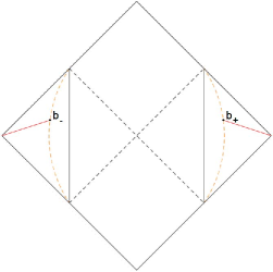
(a) without island

(b) with island

Figure 1: Penrose diagram for the black hole coupled to a thermal bath. The bath can be viewed as a non-gravitational Minkowski spacetime where $a_{\pm}$ and $b_{\pm}$ correspond to the boundaries of the island and the cutoff surface.

In order to obtain the maximal extension of the whole spacetime, we perform the Kruskal transformation, defining the following coordinates,

$$\text{ Right Wedge : }U =-e^{-\kappa\left(t-r^{*}\right)}, V=+e^{+\kappa\left(t+r^{*}\right)},$$ (2.6)

$$\text{ Left Wedge : }U =+e^{-\kappa\left(t-r^{*}\right)}, V=-e^{+\kappa\left(t+r^{*}\right)},$$

and rewrite the metric as

$$ds^{2}=-\Omega^{-2}dUdV.$$ (2.7)

For the metric in (2.3a), the twist factor $\Omega$ is given by

$$\Omega_{\text{2D}}=\frac{\kappa}{\sqrt{f(r)}}e^{\kappa r^{*}},$$ (2.8)

where $\kappa=2\pi T_{\rm{H}}$ is the surface gravity, and $r^{*}=\int f^{-1}(r)dr$ is the tortoise coordinate. For the flat bath region, $f(r)=1$, $r^{*}=r$, so we can obtain the twist factor in the bath

$$\Omega_{\text{bath}}=\kappa e^{\kappa r}.$$ (2.9)

Now, we assume the system is in a vacuum state. So we can use the entanglement entropy formula for 2D vacuum CFT [65], which reads as

$$S_{\rm{vN}}=\frac{c}{6}\log L=\frac{c}{6}\log\frac{\left(U_{1}-U_{2}\right)\left(V_{1}-V_{2}\right)}{\Omega_{1}\left(r_{1}\right)\Omega_{2}\left(r_{2}\right)},$$ (2.10)

which represents the entanglement entropy from the contribution of the matter field. Here $L$ is the geodesic distance between two boundary points of a single interval, $\Omega_{1},\Omega_{2}$ are the twist factors for these two boundary points, $U_{1,2}$ and $V_{1,2}$ are the Kruskal coordinates of these two points in the spacetime. We will use this equation to calculate the entanglement entropy in the following contexts.

3 Entanglement Entropy

In this section, we calculate the entanglement entropy of the radiation region $\left[-\infty,b_{-}\right]\cup\left[b_{+},\infty\right]$ without the contribution of the island at first. Considering the evolution of the pure state, we only need to calculate the entanglement entropy of the region $\left[b_{-},b_{+}\right]$ because of the complementarity principle, i.e. ,

$$S_{\rm{rad}}\left(\text{no island}\right)=S_{\rm{vN}}\left[b_{-},b_{+}\right]=\frac{c}{6}\log\frac{\left(U_{b_{+}}-U_{b_{-}}\right)\left(V_{b_{+}}-V_{b_{-}}\right)}{\Omega_{b_{+}}\Omega_{b_{-}}}.$$ (3.1)

Inserting $b_{+}\left(t,r_{b}\right)$ and $b_{-}\left(-t,r_{b}\right)$ into (2.6), we can obtain the Kruskal coordinates of $b_{+}$ and $b_{-}$. As shown in figure 1(a), since coordinates $b_{+}$ and $b_{-}$ are in the bath, we can obtain the twist factors by (2.9), i.e. , $\Omega_{b_{+}}=\Omega_{b_{-}}=\kappa e^{\kappa r_{b}}$. One inserts the Kruskal coordinates of $b_{+}$ and $b_{-}$ into (3.1) and obtains

$$S =\frac{c}{6}\log\frac{\left(\mathrm{e}^{\kappa(\mathrm{t}+\mathrm{r_{b}})}+\mathrm{e}^{-\kappa(\mathrm{t}-\mathrm{r_{b}})}\right)^{2}}{\kappa^{2}e^{2\kappa r_{b}}}$$ (3.2)

$$=\frac{c}{3}\log\frac{2\mathrm{cosh}\left(\kappa t\right)}{\kappa}.$$

At late times, the approximation $\kappa t\gg 1$ is valid, so we have

$$\lim_{t\to\infty}\cosh\left(\kappa t\right)\simeq\frac{1}{2}e^{\kappa t},$$ (3.3)

and then obtain,

$$S\simeq\frac{c}{3}\kappa t.$$ (3.4)

Because of the late time approximation, we can find the increase of the entanglement entropy agrees with the original Hawking’s result. The entanglement entropy grows approximately linearly with time. Therefore, there is a very sharp paradox here. The entanglement entropy diverging over time violates the unitary principle of quantum mechanics. In order to satisfy the unitary, we introduce the island to avoid such divergence.

3.1 Cutoff surface far away horizon

Now, we consider the cutoff surface that is far away from the horizon first and then consider the cutoff surface that is near the horizon for calculating the entanglement entropy with islands. The island emerges at late times as shown in figure 1(b). At large distances and late times approximation, the generalized entropy can be expressed as twice of the fine-grained entropy of the region $\left[a_{+},b_{+}\right]$ with the contribution of the island [66],

$$S_{\rm{gen}}=4\pi r_{a}+\frac{c}{3}\log\frac{\left(U_{b_{+}}-U_{a_{+}}\right)\left(V_{b_{+}}-V_{a_{+}}\right)}{\Omega_{b_{+}}\Omega_{a_{+}}},$$ (3.5)

where the first term is the area term in two-dimensional gravity and the second term represents the contribution of the matter field. $a_{+}$ and $b_{+}$ are the locations of the island and the cutoff surface in the right wedge of figure 1(b), respectively. One inserts the coordinates of $b_{+}\left(t_{b},r_{b}\right)$ and $a_{+}\left(t_{a},r_{a}\right)$ into (3.5), and obtains

$$S_{\rm{gen}}=4\pi r_{a}+\frac{c}{3}\log\frac{\sqrt{f(r_{a})}\left(2\mathrm{e}^{\kappa\left(r_{a}^{*}+\mathrm{r_{b}}\right)}\cosh\left[\kappa\left(t_{b}-t_{a}\right)\right]-\left(\mathrm{e}^{2\kappa\mathrm{r_{a}}^{*}}+\mathrm{e}^{2\kappa\mathrm{r_{b}}}\right)\right)}{\kappa^{2}e^{\kappa\left(r_{a}^{*}+r_{b}\right)}}.$$ (3.6)

At first, we extremize $S_{\rm{gen}}$ with respect to $t_{a}$, i.e.

$$\frac{\partial S_{\text{gen }}}{\partial t_{a}}=\frac{c\kappa\sinh[\kappa(t_{b}-t_{a})]}{3(\cosh[\kappa(r_{a}^{*}-r_{b})]-\cosh[\kappa(t_{b}-t_{a})])}=0.$$ (3.7)

The only solution is $t_{a}=t_{b}$. Then, (3.6) can be rewritten in the following simpler form,

$$S_{\rm{gen}}=4\pi r_{a}+\frac{2c}{3}\log\left[\frac{\mathrm{e}^{\kappa r_{b}}-\mathrm{e}^{\kappa r_{a}^{*}}}{\kappa}\right]+\frac{c}{6}\log\left[f\left(r_{a}\right)\mathrm{e}^{-2\kappa\left(r_{a}^{*}+r_{b}\right)}\right],$$ (3.8)

where $r_{a},r_{b}$ are the radial-coordinates of the island and the cutoff surface. To obtain the location of the island, we extremize $S_{\rm{gen}}$ with respect to $r_{a}$,

$$\frac{\partial S_{\text{gen }}}{\partial r_{a}}=4\pi-\frac{2c}{3}\frac{\kappa}{f\left(r_{a}\right)\left(\mathrm{e}^{\kappa\left(r_{b}-r_{a}^{*}\right)}-1\right)}+\frac{c}{6}\frac{f^{\prime}\left(r_{a}\right)-2\kappa}{f\left(r_{a}\right)}=0.$$ (3.9)

Here, we take the near horizon approximation as follows,

$$r^{*}\approx\frac{1}{2\kappa}\log\frac{r-r_{\rm{H}}}{r_{\rm{H}}},\quad f(r)\approx 2\kappa\left(r-r_{\rm{H}}\right),$$ (3.10)

where the denominator makes the whole formula dimensionless for the tortoise coordinate. By the near horizon approximation, we insert the $f\left(r_{a}\right)$ approximation into (3.9) and can be simplified as

$$\frac{12\pi}{c}=\frac{e^{\kappa r_{a}^{*}}}{\left(r_{a}-r_{\rm{H}}\right)\left(e^{\kappa r_{b}}-e^{\kappa r_{a}^{*}}\right)}-\frac{1}{2}\frac{f^{\prime}\left(r_{a}\right)-f^{\prime}\left(r_{\rm{H}}\right)}{2\kappa\left(r_{a}-r_{\rm{H}}\right)}.$$ (3.11)

Invoking $r_{a}^{*}$ approximation into (3.11), we obtain

$$\frac{12\pi}{c} =\frac{\sqrt{\frac{r_{a}-r_{\rm{H}}}{r_{\rm{H}}}}}{\left(r_{a}-r_{\rm{H}}\right)\left(e^{\kappa r_{b}}-\sqrt{\frac{r_{a}-r_{\rm{H}}}{r_{\rm{H}}}}\right)}-\frac{1}{2}\frac{f^{\prime\prime}\left(r_{\rm{H}}\right)}{2\kappa}$$ (3.12)

$$\simeq\frac{1}{\sqrt{r_{\rm{H}}\left(-r_{\rm{H}}+r_{a}\right)}\left(e^{\kappa r_{b}}-\sqrt{\frac{-r_{\rm{H}}+r_{a}}{r_{\rm{H}}}}\right)},$$

By solving (3.12), we can obtain the location of islands

$$r_{a}=r_{\rm{H}}-\frac{c}{12\pi}+\frac{1}{2}r_{\rm{H}}e^{2\kappa r_{b}}-\frac{1}{2}\sqrt{r_{\rm{H}}}e^{\kappa r_{b}}\sqrt{-\frac{c}{3\pi}+r_{\rm{H}}e^{2\kappa r_{b}}}.$$ (3.13)

Simplifying the function $r_{a}\left(c\right)$ by Taylor’s expansion in series of $c$, we obtain

$$r_{a}=r_{\rm{H}}+\frac{c^{2}}{144\pi^{2}r_{\rm{H}}}e^{-2\kappa r_{b}}+{\cal O}\left(c^{3}\right).$$ (3.14)

From (3.14), we can see that the location of the boundary of the island is outside the event horizon. We can insert (3.14) into (3.8) and omit the high order terms. We can obtain the expression of the entanglement entropy,

$$S \simeq 4\pi r_{\rm{H}}+\frac{c}{6}\log\frac{2r_{\rm{H}}}{\kappa^{3}}+{\cal O}\left(c^{2}\right)$$ (3.15)

$$\simeq 2S_{BH}.$$

Because of the emergence of islands, the entanglement entropy does not increase but arrives at a maximal value which is twice the Bekenstein-Hawking entropy. The logarithm term comes from the quantum effect of the matter field. Therefore, for the whole evaporation process, the entanglement entropy increases approximately linearly at the beginning, and then does not increase after reaching the maximum value.

3.2 Cutoff surface near horizon

Now let us discuss the case where the cutoff surface is near the horizon, which is different from the case where the cutoff surface is far from the black hole horizon. We follow the similar logic in [25]. When it nears the horizon, the generalized entropy is given by

$$S_{\rm{gen}}\simeq 4\pi r_{a}-2Kc\frac{8\pi r_{b}}{L^{2}},$$ (3.16)

where $K$ is a constant and $L$ is the geodesic distance between the endpoint of the island and the cutoff surface,

$$L \simeq\frac{1}{\sqrt{2\kappa}}\int_{r_{a}}^{r_{b}}\frac{dr}{\sqrt{r-r_{\mathrm{H}}}}$$ (3.17)

$$\simeq\frac{\sqrt{2}}{\sqrt{\kappa}}\left(\sqrt{r_{b}-r_{\rm{H}}}-\sqrt{r_{a}-r_{\rm{H}}}\right).$$

We substitute (3.17) into (3.16) and extremize $S_{\rm{gen}}$ with respect to $r_{a}$,

$$\frac{\partial S_{\text{gen }}}{\partial r_{a}}=\frac{2r_{b}c\kappa K}{\left(\sqrt{r_{b}-r_{\rm{H}}}-\sqrt{r_{a}-r_{\rm{H}}}\right)^{3}\sqrt{r_{a}-r_{\rm{H}}}}-1=0.$$ (3.18)

where approximations $\sqrt{r_{a}-r_{\rm{H}}}\ll 1$ and $r_{b}\simeq r_{\rm{H}}$ are taken into account. The minimization occurs at a smaller solution, satisfying $\sqrt{r_{a}-r_{\rm{H}}}\ll\sqrt{r_{b}-r_{\rm{H}}}$, we obtain the location of the island as

$$r_{a}=r_{\rm{H}}+\frac{\left(2r_{\rm{H}}c\kappa K\right)^{2}}{\left(r_{b}-r_{\rm{H}}\right)^{3}}.$$ (3.19)

Obviously, the location of the boundary of the island is also outside and very close to the event horizon. The result is similar to the situation that the cutoff surface is far from the horizon (3.14).

Inserting (3.19) to (3.16), we can obtain the entanglement entropy as

$$S \simeq 4\pi r_{\rm{H}}-8\pi c\kappa K\frac{r_{\rm{H}}}{r_{b}-r_{\rm{H}}}$$ (3.20)

$$\simeq 2S_{\rm{BH}}.$$

Again, the first term of the entanglement entropy is twice of the Bekenstein-Hawking entropy. The second term is a small number and can be omitted. Because of the emergence of the island, whatever we choose the cutoff surface, the entanglement entropy is about twice the Bekenstein-Hawking entropy.

In summary, the entanglement entropy without islands linear growth diverges in later times leading to the information paradox. However, once the island is considered, the configuration of space-time changes: a region that is not connected with the external radiation region appears inside the black hole, i.e., the entanglement wedge of radiation contains the black hole interior. At last, the entanglement entropy reaches a constant at late times with island. According to the island paradigm, we obtain the unitary result of the evolution of the entanglement entropy.

4 Page curve and Page time

In this section, we obtain the change of the entanglement entropy of the evolution of the black hole. At the early time, from (3.4), the entanglement entropy linearly increases. But because of the island paradigm, after the Page time, the emergence of the island leads to the entanglement entropy does not increase but is a constant (3.15). Therefore we can obtain the Page curve naturally in figure 2. By considering (3.4) and (3.15), we obtain the Page time easily,

$$t_{\text{Page }}=\frac{12\pi r_{\rm{H}}}{c\kappa}.$$ (4.1)

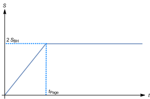
Figure 2: Page curve. The entanglement entropy linearly increases at the early time. Then after the Page time, the entanglement entropy arrives at the maximum value – twice of the Bekenstein-Hawking entropy.

Also, we can obtain the scrambling time which is defined as the minimum time interval in which the information is recovered [68]. In the island paradigm, this corresponds to the period from the cutoff surface to the boundary of the island. We assume the time interval between sending the information from the cutoff surface $r=r_{b}$ to the black hole and recovering on the island surface $r=r_{a}$ to be

$$\Delta t=r^{*}_{b}-r^{*}_{a}\simeq\frac{1}{2\kappa}\log\frac{r_{b}-r_{\rm{H}}}{r_{a}-r_{\rm{H}}}.$$ (4.2)

Substituting the value of $r_{a}$ from equation (3.14) in equation (4.2), the scrambling time is given by

$$t_{\rm{scr}}=\frac{1}{2\kappa}\log\frac{144\pi^{2}\left(r_{b}-r_{\rm{H}}\right)r_{\rm{H}}}{c^{2}e^{-2\kappa r_{b}}}\simeq\frac{1}{2\pi T_{\rm{H}}}\log S_{\rm{BH}},$$ (4.3)

where we set $r_{b}$ to have the same order with $r_{\rm{H}}$, $T_{\rm{H}}$ is the Hawking temperature defined (2.4), and $S_{\rm{BH}}=2\pi r_{\rm{H}}$ is the Bekenstein-Hawking entropy. This result is consistant with [25, 67].

5 Phase transition of the black hole

So far, we calculate the change of the entanglement entropy of the whole evaporation process for the special black hole solution and obtain the location of the island and the scrambling time. According to our calculation results, we plot the unitary Page curve. Now we consider the phase transition and analyze the relationship between the Page curve and the phase structure. We consider the charged black hole solution in canonical ensemble with $\eta=1,\zeta=2$, and set the AdS radius $l=1$. Then (2.3c) can be simplified as

$$f(r)=r^{2}-r^{2}_{\rm{H}}+a_{0}\ln\frac{r}{r_{\rm{H}}}+Q^{2}\left(r^{-1}-r^{-1}_{\rm{H}}\right).$$ (5.1)

For this charged black hole, we can obtain the Hawking temperature and the entropy from (2.4) and (2.5), which read as

$$T_{\rm{H}}=\frac{2r_{\rm{H}}^{3}+a_{0}r_{\rm{H}}-Q^{2}}{4\pi r_{\rm{H}}^{2}},\quad S=2\pi r_{\rm{H}}.$$ (5.2)

We also can obtain the expression of the free energy of this black hole solution [62],

$$F=-\frac{1}{2}r_{\rm{H}}^{2}-\frac{Q^{2}}{2}r_{\rm{H}}^{-1}-\frac{a_{0}}{2}+\frac{a_{0}}{2}\ln r_{\rm{H}}.$$ (5.3)

In the following, we study the chargeless case first and then consider the charged black hole.

5.1 $Q=0$

For the special case with $Q=0$, the black hole thermodynamics phase diagram reduces to the Hawking-Page phase transition. We can write down the Hawking temperature and the free energy as

$$T_{\rm{H}}=\frac{r_{\rm{H}}}{2\pi}+\frac{a_{0}}{4\pi r_{\rm{H}}},\quad F=-\frac{1}{2}r_{\rm{H}}^{2}-\frac{a_{0}}{2}+\frac{a_{0}}{2}\ln r_{\rm{H}}.$$ (5.4)

At the same temperature, for the small black hole, its horizon radius is

$$r_{s}=\frac{1}{2}\left(2\pi T_{\rm{H}}-\sqrt{2}\sqrt{-a_{0}+2\pi^{2}T_{\rm{H}}^{2}}\right),$$ (5.5)

while, for the large black hole, its horizon radius is

$$r_{l}=\frac{1}{2}\left(2\pi T_{\rm{H}}+\sqrt{2}\sqrt{-a_{0}+2\pi^{2}T_{\rm{H}}^{2}}\right).$$ (5.6)

Obviously, there is a minimum temperature $T_{\rm{H}\left(\rm{min}\right)}=\frac{\sqrt{a_{0}}}{\sqrt{2}\pi}$. For the minimum temperature, two radii are coincident, $r_{l}=r_{s}=\frac{\sqrt{a_{0}}}{\sqrt{2}}$. Moreover, there are no black hole phases below the minimum temperature.

We can plot the $F$-$T_{\rm{H}}$ diagram as follows.

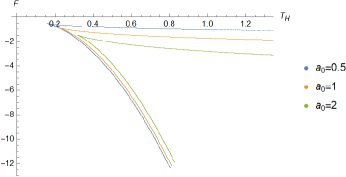
Figure 3: The free energy $F$ as a function of temperature $T_{\rm{H}}$ at $a_{0}=0.5,1,2$. The situation of the Hawking-Page phase structure. The low and high branches correspond to the large and small black holes.

As shown in figure 3, the free energy of the large black hole is always lower than the free energy of the small black hole. Therefore, for the same temperature, the large black hole is the stable phase. Considering the Hawking-Page phase transition, the small black hole is thermodynamically unstable. Therefore, we do not need to consider the island and the Page time of the small black hole, including the extremal black hole.

To study the effect on the Page curve from the Hawking-Page phase transition, we consider the situation in the absence of the islands first. From equation (3.4), the entanglement entropy increases linearly at late times. As shown in figure 4, we obtain the figure for the increased rate of the entanglement entropy and the Page time,

$$\frac{S}{t}=\frac{c}{3}\kappa.$$ (5.7)

We choose $\eta=1,\zeta=2,Q=0,c=1.5$ for (4.1) and (4.2), then we obtain

$$t_{\text{Page }}=\frac{16\pi}{2+a_{0}r_{\rm{H}}^{-2}},\quad t_{\text{scr}}=\frac{2r_{\rm{H}}}{2r_{\rm{H}}^{2}+a_{0}}\log 2\pi r_{\rm{H}}.$$ (5.8)

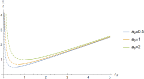
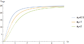
Figure 4: The increased rate of the entanglement entropy and the Page time as a function for the radius at $a_{0}=0.5,1,2$. The dotted line represents the unstable small black hole.

Now we consider the island paradigm,

$$S_{\mathrm{rad}}\left(r_{\mathrm{H}},t\right)=\text{Min}\left[S\left(\text{no island}\right),S\left(\text{with island}\right)\right]=\text{Min}\left[\frac{c}{3}\log\frac{2\cosh(\kappa t)}{\kappa},2S_{\mathrm{BH}}\right].$$ (5.9)

The whole process of the evolution of the entanglement entropy should satisfy (5.9). Considering the Hawking-Page phase transition, we set $c=1.5$ and plot the Page curve as a function of time $t$ and radius $r_{\rm{H}}$ for $a_{0}=1$ in figure 6.

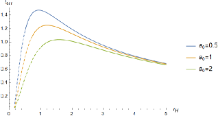
Figure 5: The scrambling time as a function for the radius at $a_{0}=0.5,1,2$. The dotted line represents the unstable small black hole.

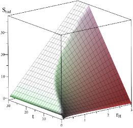
Figure 6: Page curves as a function of time $t$ and radius $r_{\rm{H}}$ for $a_{0}=1$ and $c=1.5$.

5.2 $Q\neq 0$

For the general case, we set $\eta=1,\zeta=2,a_{0}=1,l=1$ and obtain the Hawking temperature and the free energy as

$$T_{\mathrm{H}}=\frac{2r_{\mathrm{H}}^{3}+r_{\mathrm{H}}-Q^{2}}{4\pi r_{\mathrm{H}}^{2}},\quad F=-\frac{1}{2}r_{\mathrm{H}}^{2}-\frac{Q^{2}}{2}r_{\mathrm{H}}^{-1}-\frac{1}{2}+\frac{1}{2}\ln r_{\mathrm{H}}.$$ (5.10)

By extremizing $T_{\rm{H}}$ with respect to $r_{\rm{H}}$,

$$\frac{\partial T_{\rm{H}}}{\partial r_{\rm{H}}}=2r_{\rm{H}}^{3}-r_{\rm{H}}+2Q^{2} =0,$$ (5.11)

we can find only two real, positive solutions obey (5.11). These two solutions coalesce at the critical point,

$$\frac{\partial^{2}T_{\rm{H}}}{\partial^{2}r_{\rm{H}}}=r_{\rm{H}}-3Q^{2}=0.$$ (5.12)

According to equations (5.11) and (5.12), we can obtain $r_{\rm{H}\left(\text{crit}\right)}=\frac{1}{\sqrt{6}}$, $Q_{\left(\text{crit}\right)}=\frac{1}{\sqrt{3\sqrt{6}}}$, $T_{\rm{H}\left(\text{crit}\right)}=\frac{1}{2\pi}\sqrt{\frac{3}{2}}$. Also, we can plot the $F$-$T_{\rm{H}}$ diagram for the charged situation as follows.

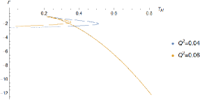
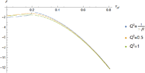
Figure 7: (a): The free energy $F$ as a function of temperature $T_{\rm{H}}$ at $Q^{2}=0.04,0.06$. (b): The free energy $F$ as a function of temperature $T_{\rm{H}}$ at $Q^{2}=Q^{2}_{\text{ crit }},0.5,1$.

There is a section of the well-known “swallowtail” shape in figure 7. The intersection points correspond to the phase transition point in the fixed charge ensemble for $Q^{2}<Q^{2}_{\rm{crit}}$. The most stable phase requires the lowest free energy. When $Q^{2}>Q^{2}_{\rm{crit}}$, the swallowtail structure disappears in figure 7, so the phase transition also does not happen.

To investigate the phase transition effects on the Page curve, we plot the increased rate of the entanglement entropy as a function of the radius for several different values of $Q^{2}$,

$$\frac{S}{t}=\frac{c}{3}\kappa=\frac{2r_{\rm{H}}^{3}+r_{\rm{H}}-Q^{2}}{2r_{\rm{H}}^{2}}.$$ (5.13)

According to (4.1) and (4.3), we set $c$=1.5 and write down the Page time and the scrambling time versus the radius for any $Q^{2}$,

$$t_{\text{Page }} =\frac{16\pi}{2+r_{\rm{H}}^{-2}-Q^{2}r_{\rm{H}}^{-3}},$$ (5.14)

$$t_{\text{scr }} =\frac{2r_{\rm{H}}^{2}}{2r_{\rm{H}}^{3}+r_{\rm{H}}-Q^{2}}\log 2\pi r_{\rm{H}}.$$

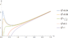
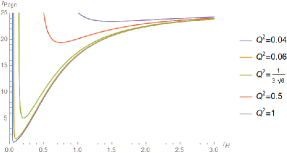
Figure 8: The increased rate of the entanglement entropy and the Page time as a function for the radius at $Q^{2}=0.04,0.06,\frac{1}{3\sqrt{6}},0.5,1$.

Obviously, in figure 8, the increased rate of the entanglement entropy is not a monotonic function of the radius when $Q^{2}<Q^{2}_{\rm{crit}}$. The same increased rate corresponds to three different radius values which represent the “small, middle, large” black hole. However, in real physical processes, the lower the free energy is, the more stable phase is. As figure 7, the intersection points are just the critical points where the phase transition happens. Above the critical temperature, the large black hole is more stable, but below the critical temperature, the small black hole is more stable. Thus, figure 7 behaves like the van der Waals-Maxwell phase structure.

In figure 8, it is obvious that the Page time will be a constant $\left(t_{\rm{Page}}=8\pi\right)$, when $r_{\rm{H}}$ approaches infinity. For the large black hole, the charge and entropy do not influence the Page time. However, for the extremal black hole, the Page time is divergent. Since the middle black hole is unstable, so that the physical meaning of the Page time of the middle black hole is not clear when $Q^{2}<Q^{2}_{\rm{crit}}$.

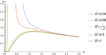
Figure 9: The scrambling time as a function for the radius at $Q^{2}=0.04,0.06,\frac{1}{3\sqrt{6}},0.5,1$.

Considering the island paradigm (5.9), we set $c=1.5$ and plot the Page curve of a series of small and large black holes at $Q^{2}=0.04$ in figure 10. As shown in figure 10, for the small black hole, the Page time approaches zero. It is different from figure 8. Because we take the late time approximation in figure 8, it is inaccurate for the Page time of the small black hole. But we do not use the late time approximation in (5.9), therefore the result of figure 10 is reasonable.

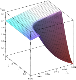
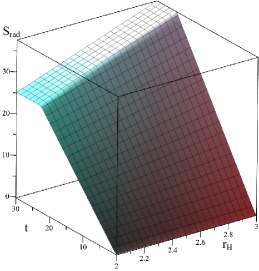
Figure 10: Page curves for different black holes with $c=1.5$. (a): Page curves as a function of time $t$ and radius $r_{\rm{H}}$ for a series of the small black hole at $Q^{2}=0.04$. (b): Page curves as a function of time $t$ and radius $r_{\rm{H}}$ for the large black hole at $Q^{2}=0.04$.

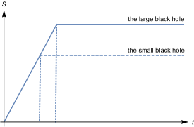
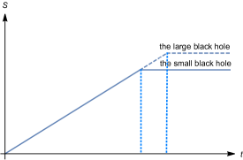
Figure 11: Page curves for different temperatures. (a): Page curve at the temperature which is higher than the critical temperature. (b): Page curve at the temperature which is lower than the critical temperature.

In figure 11, we plot the Page curve of the black hole with the special phase structure. Above the critical temperature, we can only obtain the Page curve of the large black hole. However, below the critical temperature, we can only obtain the Page curve of the small black hole. The lower the temperature, the greater the Page time. This implies that the lower the temperature, the later the island appears in the black hole’s interior.

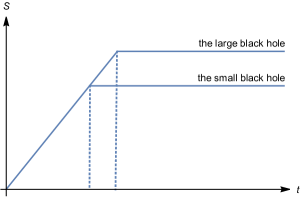
Figure 12: Page curve for the critical temperature. The large and small black holes coexist.

Taking into account the critical temperature, because of the instability of the middle black hole, the range of the radius of the middle black hole would not become the black hole phase, so the island does not emerge. As the phase transition of the black hole, the location of the island also has a jump. In figure 12, when the black hole temperature is the critical temperature, the large and small black holes coexist.

Finally, we consider the different situations without phase transition when $Q^{2}>Q^{2}_{\rm{crit}}$. The green branch corresponds to the critical charge in figure 8. As shown in figure 8, we know the increased rate of the entanglement entropy beyond the critical charge is the monotone function of the radius. As shown in figure 8, with the increase of the charge, the Page time is later. There is no more phase transition, so the Page curve has no special situation for any size black hole just like in figure 2. We set $c=1.5$ and plot the Page curve as a function of time $t$ and radius $r_{\rm{H}}$ at $Q^{2}=0.5$ in figure 13.

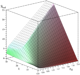
Figure 13: Page curves as a function of time $t$ and radius $r_{\rm{H}}$ at $Q^{2}=0.5$ and $c=1.5$.

6 Discussion and Conclusion

In summary, we consider the information paradox for a special black hole derived from the deformed JT gravity with the van der Waals-Maxwell like phase structure. To make the black hole evaporate, we construct the eternal black hole by gluing the flat bath. Then we use the island formula to calculate the entanglement entropy. At early time, the entanglement entropy linearly increases without islands. It matches Hawking’s original calculations. At later times, because of the island, the entanglement entropy reaches a constant value which is twice of the Bekenstein-Hawking entropy. Finally, we obtain the scrambling time and the Page curve. We obtain the unitary result and the island outside the event horizon that is consistent with the result of the eternal black hole. Moreover, we consider different situations for the cutoff surface and find the final result is independent of the distance of the cutoff surface.

Moreover, we consider the impact of the phase transition. Phase transition is an important and interesting thermodynamic phenomenon. In fixed charged ensembles with different charges, the black hole has different phase transitions. There is the Hawking-Page phase transition in the black hole without charges. As the charge increases, There is the van der Waals-Maxwell-like phase transition. But if the charge is beyond the critical charge, there are no phase transitions. We study the island and the Page time for the black hole with these phase structures to obtain some results about the influence yielded on the phase transition.

For an neutral black hole without charges, there is only the Hawking-Page phase transition. For the same temperature, there are two black hole phases – the small and large black holes. By calculating the free energy and the Hawking temperature, we obtain figure 3, where the large black hole with lower free energy is more stable. Note that the system has a minimum temperature for forming the black hole. So it is meaningless to discuss the island and the Page time below this minimum temperature in this situation. Thus, we only can obtain the Page curve of the large black hole.

For charged black holes, at first, we consider $Q<Q_{\rm{crit}}$, the black hole would have the van der Waals-Maxwell-like phase structure that three different black hole phases may correspond to the same temperature. By calculating the free energy and the Hawking temperature, we obtain figure 7, the lowest free energy phase is stable, so only one of the three phases is the stable one. There is a critical temperature where the small black hole phase would jump to the large black hole phase. Of course, the Page time about the middle black hole is meaningless. The situations with the temperature beyond, below, and equal to the critical temperature respectively correspond to figure 11 which the large black hole is more stable, figure 11 which the small black hole is more stable, and figure 12 which the small and large black holes coexist. Then we consider $Q\geq Q_{\rm{crit}}$ case in which is the no phase transition happens. The Page time for any temperature is well defined in this situation. Different from the no phase transition situation, the Page time of the small black hole approaches zero in figure 10. We do not use the late time approximation to calculate the Page time in (5.9). The scrambling time curve monotonically decreases in the no phase transition situation. But in the phase transition situation, there is a maximum scrambling time.

In the doubly-holographic system [69], one simply includes a second Karch-Randall brane as a gravitating bath. One finds if the bath itself gravitates, the original Page curve vanishes. And the quantum extremal surface is just at the horizon. These successful works about the introduction of the gravitating bath are in the high dimension [69, 31, 70]. But there is no graviton in two dimensions. So we can not introduce the KR brane as the gravitating bath in our 2d gravity model. We will consider the reliable construction of the gravitating bath in future work.

In conclusion, we use a simple black hole model with a rich phase structure to compute and analyze the Page curve and study the effect of the phase transition to Page curves. We find the important relationship between the phase transition and the black hole information paradox. We hope that the deep understanding and keen insight of the 2D gravity model in this paper can be applied to the higher-dimensional space-time we live in. As an important phenomenon, the phase transition might be interesting for understanding the information paradox.

References

- [1] S. W. Hawking, “Particle Creation by Black Holes,” Commun. Math. Phys. 43, 199 (1975). Erratum;[Commun. Math. Phys. 46, 206 (1976)].
- [2] S. W. Hawking, “Breakdown of Predictability in Gravitational Collapse,” Phys. Rev. D 14, (1976) 2460-2473.
- [3] D. N. Page, “Information in black hole radiation,” Phys. Rev. Lett. 71, 3743-3746 (1993) [arXiv:hep-th/9306083 [hep-th]].
- [4] D. N. Page, “Time Dependence of Hawking Radiation Entropy,”JCAP 1309, 028 (2013) [arXiv:1301.4995 [hep-th]].
- [5] N. Engelhardt and A. C. Wall, “Quantum Extremal Surfaces: Holographic Entanglement Entropy beyond the Classical Regime,”JHEP 01, 073 (2015), [arXiv:1408.3203 [hep-th]].
- [6] A. Almheiri, R. Mahajan, J. Maldacena and Y. Zhao, “The Page curve of Hawking ridiation from semiclassical geometry,”JHEP 03, 149 (2020) [arXiv:1908.10996[hep-th]].
- [7] G. Penington, “Entanglement Wedge Reconstruction and the Information Paradox,”JHEP 09 002 (2020) [arXiv:1905.08255[hep-th]].
- [8] A. Almheiri, N. Engelhardt, D. Marolf and H. Maxfield, “The entropy of bulk quantum fields and the entanglement wedge of an evaporating black hole,”JHEP 12, 063 (2019) [arXiv:1905.08762[hep-th]].
- [9] A. Almheiri, R. Mahajan and J. Maldacena, “Islands outside the horizon,”[arXiv:1910.11077 [hep-th]]
- [10] T. Hollowood and S. Kumar, “Islands and Page Curves for Evaporating Black Holes in JT Gravity,”[arXiv:2004.14944[hep-th]].
- [11] H. Chen, Z. Fisher, J. Hernandez, R. Myers and S. Ruan, “Information Flow in Black Hole Evaporation,”JHEP 03, 152 (2020) [arXiv:1911.03402[hep-th]].
- [12] H. Chen, Z. Fisher, J. Hernandez, R. Myers and S. Ruan, “Evaporating Black Holes Coupled to a Thermal Bath,” [arXiv:2007.11658[hep-th]].
- [13] A. Almheiri, T. Hartman, J. Maldacena, E. Shaghoulian and A. Tajdini, “Replica Wormholes and the Entropy of Hawking Radiation,”[arXiv:1911.12333[hep-th]].
- [14] E. Verheijden and E. Verlinde, “From the BTZ black hole to JT gravity: geometrizing the island,”JHEP 11 (2021) 092 [arXiv:2102.00922[hep-th]].
- [15] Song He, Yuan Sun, Long Zhao and Yu-Xuan Zhang, “The universality of islands outside the horizon,” [arXiv:2110.07598 [hep-th]].
- [16] Po-Chun Sun, “Entanglement Islands from Holographic Thermalization of Rotating Charged Black Hole,” [arXiv:2108.12557 [hep-th]].
- [17] Ming-Hui Yu, Cheng-Yuan Lu, Xian-Hui Ge and Sang-Jin Sin, “Island, Page Curve and Superradiance of Rotating BTZ Black Holes,” Phys.Rev.D 105 (2022) 6, 066009 [arXiv:2112.14361 [hep-th]].
- [18] Ming-Hui Yu and Xian-Hui Ge, “Entanglement Islands in Generalized Two-dimensional Dilaton Black Holes,” [arXiv:2208.01943[hep-th]].
- [19] T. Anegawa and N. Iizuka, “Notes on islands in asymptotically flat 2d dilaton black holes,” JHEP 07, 036 (2020) [arXiv:2004.01601[hep-th]].
- [20] T. Hartman, E. Shaghoulian and A. Strominger, “Islands in Asymptotically Flat 2D Gravity,” JHEP 07, 022 (2020) [arXiv:2004.13857[hep-th]].
- [21] K. Goto, T. Hartman and A. Tajdini, “Replica wormholes for an evaporating 2D black hole,” [arXiv:2011.09043[hep-th]].
- [22] Xuanhua Wang, Ran Li and Jin Wang, “Page curves for a family of exactly solvable evaporating black holes,” [arXiv:2104.00224[hep-th]].
- [23] Ran Li, Xuanhua Wang and Jin Wang, “Island may not save the information paradox of Liouville black holes,”[arXiv:2105.03271[hep-th]].
- [24] Ming-Hui Yu and Xian-Hui Ge, “Page Curves and Islands in Charged Dilaton Black Holes,” Eur.Phys.J.C 82 (2022) 2, 167[arXiv:2107.03031 [hep-th]].
- [25] K. Hashimoto, N. Iizuka and Y. Matsuo, “Islands in Schwarzschild black holes,” JHEP 06, 085 (2020) [arXiv:2004.05863 [hep-th]].
- [26] A. Almheiri, R. Mahajan and J. E. Santos, “Entanglement islands in higher dimensions,”SciPost Phys. 9, no.1, 001 (2020) [arXiv:1911.09666 [hep-th]].
- [27] S. A. Hosseini Mansoori, O. Luongo, S. Mancini, M. Mirjalali, M. Rafiee and A. Tavanfar, “Planar Black Holes in Holographic Axion Gravity: Islands, Page Times, and Scrambling Times,” [arXiv:2209.00253 [hep-th]].
- [28] Y. Ling, Y. Liu and Z. Xian, “Island in charged black holes,” JHEP 03, 251 (2021) [arXiv:2010.00037[hep-th]].
- [29] M. Alishahiha, A. Astaneh and A. Naseh, “Island in the presence of higher derivative terms,” JHEP 02, 035 (2021) [arXiv:2005.08715[hep-th]].
- [30] Y. Matsuo, “Islands and stretched horizon,” JHEP 07, 051 (2021) [arXiv:2011.08814[hep-th]].
- [31] H. Geng and A. Karch, “Massive islands,” JHEP 09, 121 (2020) [arXiv:2006.02438 [hep-th]].
- [32] J. Chu, F. Deng and Y. Zhou, “Page Curve from Defect Extremal Surface and Island in Higher Dimensions,” JHEP 10, 149 (2021) [arXiv:2105.09106[hep-th]].
- [33] K. Ghosh and C. Krishnan, “Dirichlet baths and the not-so-fine-grained Page curve,”JHEP 08, 119 (2021) [arXiv:2103.17253 [hep-th]].
- [34] Gopal Yadav, “Page Curves of Reissner-Nordström Black Hole in HD Gravity,”Eur. Phys. J. C 82, 904 (2022).
- [35] T. Hartman, Y. Jiang and E. Shaghoulian, “Islands in cosmology,” JHEP 11, 111 (2020) [arXiv:2008.01022[hep-th]].
- [36] V. Balasubramanian, A. Kar and T. Ugajin, “Islands in de Sitter space,” JHEP 02, 072 (2021) [arXiv:2008.05275[hep-th]].
- [37] S. Azarnia, R. Fareghbal, A. Naseh and H. Zolfi, “Islands in Flat-Space Cosmology,” [arXiv:2109.04795[hep-th]].
- [38] Kaberi Goswami, K. Narayan and Hitesh K. Saini. “Cosmologies, singularities and quantum extremal surfaces,”[arXiv:2111.14906[hep-th]].
- [39] Ricardo Espindola, Bahman Najian and Dora Nikolakopoulou, “Islands in FRW Cosmologies,” [arXiv:2203.04433[hep-th]].
- [40] Gopal Yadav and Nitin Joshi, “Cosmological and black hole Islands in multi-event horizon spacetimes,” [arXiv:2210.00331[hep-th]].
- [41] Raphael Bousso and Elizabeth Wildenhain, “Islands in Closed and Open Universes,” [arXiv:2202.05278[hep-th]].
- [42] Joshua Kames-King, Evita Verheijden and Erik Verlinde, “No Page Curves for the de Sitter Horizon,” [arXiv:2108.09318 [hep-th]].
- [43] Kenta Suzuki and Tadashi Takayanagi, “BCFT and Islands in Two Dimensions,” [arXiv:2202.08462 [hep-th]].
- [44] Zhi Wang, Zekun Xu, Shuyan Zhou and Yang Zhou, “Partial Reduction and Cosmology at Defect Brane,” [arXiv:2112.13782 [hep-th]].
- [45] Qi-Lin Hu, Dongqi Li, Rong-Xin Miao and Yu-Qian Zeng, “AdS/BCFT and Island for curvature-squared gravity,” [arXiv:2202.03304[hep-th]].
- [46] T. Li, J. Chu and Y. Zhou, “Reflected Entropy for an Evaporating Black Hole,” JHEP 11, 155 (2020) [arXiv:2006.10846[hep-th]].
- [47] Ahmed Almheiri and Henry W. Lin, “The Entanglement Wedge of Unknown Couplings,” [arXiv:2111.06298[hep-th]].
- [48] T. Li, M. Yuan and Y. Zhou, “Defect Extremal Surface for Reflected Entropy,” [arXiv:2108.08544[hep-th]].
- [49] Dmitry S. Ageev, “Shaping contours of entanglement islands in BCFT,” [arXiv:2108.08544[hep-th]].
- [50] Yiming Chen, Xiao-Liang Qi and Pengfei Zhang, “Replica wormhole and information retrieval in the SYK model coupled to Majorana chains,” [arXiv:2003.13147[hep-th]].
- [51] Shao-Kai Jian and Brian Swingle, “Note on entropy dynamics in the Brownian SYK model,” [arXiv:2011.08158 [hep-th]].
- [52] Daniel L. Nedel, “Time dependent Entanglement Entropy in SYK models and Page Curve,” [arXiv:2007.06770 [hep-th]].
- [53] Kaixiang Su, Pengfei Zhang and Hui Zhai, “Page curve from non-Markovianity,” [arXiv:2101.11238 [hep-th]].
- [54] A. Kruchkov, A. Patel, P. Kim and S.r Sachdev, “Thermoelectric power of Sachdev-Ye-Kitaev islands: Probing Bekenstein-Hawking entropy in quantum matter experiments,” [arXiv:1912.02835[hep-th]].
- [55] G. Penington, S. H. Shenker, D. Stanford and Zhenbin Yang, “Replica wormholes and the black hole interior,” [arXiv:1911.11977[hep-th]].
- [56] R. Jackiw, “Lower dimensional gravity,” Nuclear Physics B 252 (1985): 343-356.
- [57] C. Teitelboim, “Gravitation and hamiltonian structure in two spacetime dimensions,” Physics Letters B 126.1-2 (1983): 41-45.
- [58] E.Witten, “Matrix models and deformations of JT gravity,” Proceedings of the Royal Society A 476.2244 (2020): 20200582.
- [59] Davood Momeni and Phongpichit Channuie, “Exact Solutions of (deformed) Jackiw-Teitelboim Gravity,” Eur.Phys.J. C 81 (2021) no.6, 534 [arXiv:2009.03723 [hep-th]].
- [60] M.Alishahiha, A.Faraji Astaneh, G.Jafari, A.Naseh and B.Taghavi, “Free energy for deformed Jackiw-Teitelboim gravity.” Phys. Rev. D 103.4 (2021): 046005.
- [61] D.Momeni, “Real classical geometry with arbitrary deficit parameter (s) in deformed Jackiw-Teitelboim gravity,” Eur.Phys.J.C 81 (2021) 3, 202.
- [62] Sizheng Cao, Yi-Cheng Rui and Xian-Hui Ge, “Thermodynamic phase structure of complex Sachdev-Ye-Kitaev model and charged black hole in deformed JT gravity,” [arXiv:2103.16270[hep-th]].
- [63] Wei Sun and Xian-Hui Ge, “Holographic heat engine efficiency of hyperbolic charged black holes,” Chinese Physics B 30.10 (2021): 109501[arXiv:2205.00654[gr-qc]].
- [64] Wenhe Cai, Sizheng Cao, Xian-Hui Ge, Masataka Matsumoto and Sang-Jin Sin, “A Non-Hermitian two coupled Sachdev-Ye-Kitaev model,” [arXiv:2208.10800[hep-th]].
- [65] P. Calabrese and J. Cardy, “Entanglement entropy and conformal field theory,” J. Phys.A42 (2009) 504005 [arXiv:0905.4013[hep-th]].
- [66] H. Casini, C. D. Fosco and M. Huerta, “Entanglement and alpha entropies for a massive Dirac field in two dimensions,” J.Stat.Mech.0507:P07007,2005[arXiv:cond-mat/0505563 [cond-mat.other]].
- [67] Qing-Bing Wang, Ming-Hui Yu and Xian-Hui Ge, “ Scrambling time for analogue black holes embedded in AdS space,” Eur. Phys. J. C 82 (2022) 468 [arXiv:2203.07914[hep-th]].
- [68] P.Caputa, J.Simon, A.Stikonas, T.Takayanagi and K. Watanabe, “ Scrambling time from local perturbations of the eternal BTZ black hole,” [arXiv:1503.08161[hep-th]].
- [69] Hao Geng, Andreas Karch, Carlos Perez-Pardavila, Suvrat Raju, Lisa Randall, Marcos Riojas and Sanjit Shashi, “ Information Transfer with a Gravitating Bath,” SciPost Physics 10.5 (2021): 103 [arXiv:2012.04671 [hep-th]].
- [70] Hao Geng, Severin Lüst, Rashmish K. Mishra and David Wakeham, “ Holographic BCFTs and Communicating Black Holes,” JHEP 08 (2021) 003 [arXiv:2104.07039 [hep-th]].