Monotonic segmental attention for automatic speech recognition

Abstract

We introduce a novel segmental-attention model for automatic speech recognition. We restrict the decoder attention to segments to avoid quadratic runtime of global attention, better generalize to long sequences, and eventually enable streaming. We directly compare global-attention and different segmental-attention modeling variants. We develop and compare two separate time-synchronous decoders, one specifically taking the segmental nature into account, yielding further improvements. Using time-synchronous decoding for segmental models is novel and a step towards streaming applications. Our experiments show the importance of a length model to predict the segment boundaries. The final best segmental-attention model using segmental decoding performs better than global-attention, in contrast to other monotonic attention approaches in the literature. Further, we observe that the segmental model generalizes much better to long sequences of up to several minutes.

Index Terms—  Segmental attention, segmental models

1 Introduction & related work

The attention-based encoder-decoder architecture [1] has been very successful as an end-to-end model for many tasks including speech recognition [2, 3, 4, 5, 6]. However, for every output label, the attention weights are over all the input frames, referred to as global attention. This has the drawbacks of quadratic runtime-complexity, potential non-monotonicity; it does not allow for online streaming recognition and it does not generalize to longer sequence lengths than those seen in training [7, 8, 9].

There are many attempts to solve some of these issues. Monotonic chunkwise attention (MoChA) [10, 11, 12] is one popular approach which uses fixed-size chunks for soft attention and a deterministic approach for the chunk positions, i.e. the position is not treated as a latent variable in recognition. Many similar approaches using a local fixed-sized window and some heuristic or separate neural network for the position prediction were proposed [2, 13, 14, 15, 16, 17, 18, 19, 20]. The attention sometimes also uses a Gauss distribution which allows for a differentiable position prediction [21, 22, 14, 15, 16]. Some models add a penalty in training, or are extended to have an implicit bias to encourage monotonicity [23, 2, 13]. Framewise defined models like CTC [24] or transducers [25] canonically allow for streaming, and there are approaches to combine such framewise model with attention [26, 27, 28, 29, 30, 31, 32, 33].

Our probabilistic formulation using latent variables for the segment boundaries is similar to other segmental models [34, 35, 36, 37, 38, 39, 40, 41, 42, 43, 44, 45, 46], although attention has not been used on the segments except in [46] and there are usually more independence assumptions such as first or zero order dependency on the label, and only a first order dependency on the segment boundary, which is a critical difference. It has also been shown that transducer models and segmental models are equivalent [47].

Here, we want to make use of the attention mechanism while solving the mentioned global attention drawbacks by making the attention local and monotonic on segments. We treat the segment boundaries as latent variables and end up at our segmental attention models. Such segmental models by definition are monotonic, allow for streaming, and are much more efficient by using only local attention. Our aim is to get a better understanding of such segmental attention models, to directly compare it to the global attention model, to study how to treat and model the latent variable, how to perform the search for recognition, how to treat silence, how well it generalizes to longer sequences among other questions.

2 Global attention model

Our starting point is the standard global-attention-based encoder-decoder model [1] adapted for speech recognition [2, 3, 5, 6], specifically the model as described in [4, 48, 49]. We use an LSTM-based [50] encoder which gets a sequence of audio feature frames $x_{1}^{T^{\prime}}$ of length $T^{\prime}$ as input and encodes it as a sequence

$$h_{1}^{T}=\operatorname{Encoder}(x_{1}^{T^{\prime}})$$

of length $T$, where we apply downsampling by max-pooling in time inside the encoder by factor 6. For the output label sequence $a_{1}^{S}$ of length $S$, given the encoder output sequence $h_{1}^{T}$ of length $T$, we define

$$p(a_{1}^{S}\mid h_{1}^{T}) =\prod_{s=1}^{S}\underbrace{p(a_{s}\mid a_{1}^{s-1},h_{1}^{T})}_{\text{label model}},$$

The label model uses global attention on $h_{1}^{T}$ per each output step $s$. The neural structure which defines the probability distribution of the labels is also called the decoder. The decoder of the global-attention model is almost the same as our segmental attention model, which we will define below in detail. The main difference is segmental vs. global attention.

3 Our segmental attention model

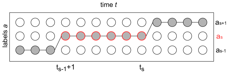
Fig. 1: Example alignment of label sequence $...a_{s-1}a_{s}a_{s+1}...$. Segment for $a_{s}$ highlighted.

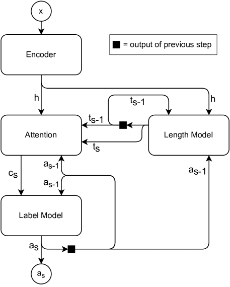
Fig. 2: Segmental attention model

Now, we introduce segment boundaries as a sequence of latent variables $t_{1}^{S}$. Specifically, for one output $a_{s}$, the segment is defined by $[t_{s-1}+1,t_{s}]$, with $t_{0}=0$ and $t_{S}=T$ fixed, and we require $t_{s}>t_{s-1}$ for strict monotonicity. Thus, the segmentation fully covers all frames of the sequence. One such segment is highlighted in Figure 1. The label model now uses attention only in that segment, i.e. on $h_{t_{s-1}+1}^{t_{s}}$. For the output label sequence $a_{1}^{S}$, we now define the segmental model as

$$p(a_{1}^{S}\mid h_{1}^{T}) =\sum_{t_{1}^{S}}\prod_{s=1}^{S}\underbrace{p(t_{s}\mid...\vphantom{h_{t_{s-1}+1}^{t_{s}}})^{\alpha}}_{\text{length model}}\cdot\underbrace{p(a_{s}\mid a_{1}^{s-1},h_{t_{s-1}+1}^{t_{s}},...)}_{\text{label model}}.$$

In the simplest case, we even do not use any length model ($\alpha=0$). The intuition was that a proper dynamic search over the segment boundaries can be guided by the label model alone, as it should produce bad scores for bad segment boundaries. We also test a simple static length model, and a neural length model, as we will describe later. The label model is mostly the same as in the global attention case with the main difference that we have the attention only on $h_{t_{s-1}+1}^{t_{s}}$. The whole segmental model is depicted in Figure 2.

3.1 Label model variations

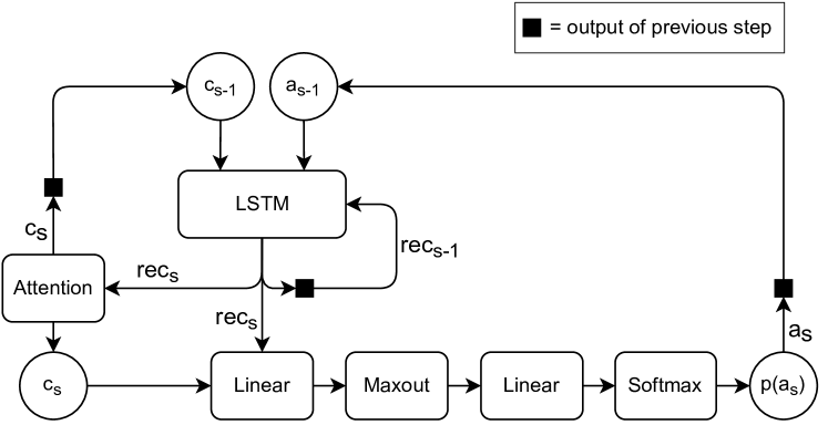
Fig. 3: Segmental attention label model $p(a_{s}|...)$

The label model is depicted in Figure 3 and defined as

$$p(a_{s}\mid...) =(\operatorname{softmax}\circ\operatorname{Linear}\circ\operatorname{maxout}\circ\operatorname{Linear})\big{(}$$

$$\quad\quad(\operatorname{LSTM}({\color[rgb]{0,0,1}\bm{c_{1}^{s-1}}},a_{1}^{s-1}),c_{s})\big{)}$$

$$c_{s} =\sum_{t={\color[rgb]{1,0,0.87}\bm{t_{s-1}+1}}}^{{\color[rgb]{1,0,0.87}\bm{t_{s}}}}\alpha_{s,t}\cdot h_{t}$$

$$\alpha_{s,t} =\frac{\exp(e_{s,t})}{\sum_{\tau={\color[rgb]{1,0,0.87}\bm{t_{s-1}+1}}}^{{\color[rgb]{1,0,0.87}\bm{t_{s}}}}\exp(e_{s,\tau})}$$

$$e_{s,t} =(\operatorname{Linear}\circ\tanh\circ\operatorname{Linear})\big{(}$$

$$\quad\quad(\operatorname{LSTM}({\color[rgb]{0,0,1}\bm{c_{1}^{s-1}}},a_{1}^{s-1}),h_{t})\big{)}.$$

The attention weights here are only calculated on the interval $[{\color[rgb]{1,0,0.87}\bm{t_{s-1}+1}},{\color[rgb]{1,0,0.87}\bm{t_{s}}}]$. Further, we do not have attention weight feedback as there is no overlap between the segments. Otherwise the model is exactly the same as the global attention decoder, to allow for direct comparisons, and also to import model parameters.

Another variation is on the dependencies. In any case, we depend on the full label history $a_{1}^{s-1}$. When we have the dependency on ${\color[rgb]{0,0,1}\bm{c_{1}^{s-1}}}$ as it is standard for LSTM-based attention models, this implies an implicit dependency on the whole past segment boundaries $t_{1}^{s-1}$, which removes the option of an exact first-order dynamic programming implementation for forced alignment or exact sequence-likelihood training. So, we also test the variant where we remove the ${\color[rgb]{0,0,1}\bm{c_{1}^{s-1}}}$ dependency in the equations above.

3.2 Silence modeling

The output label vocabulary of the global attention model usually does not include silence as this is not necessarily needed. Our segments completely cover the input sequence, and thus the question arises whether the silence parts should be separate segments or not, i.e. whether we should add silence to the vocabulary. Additionally, as silence segments tend to be longer, we optionally split them up. We will perform experiments for all three variants, also for the global attention model.

Further, when we include silence, the question is whether this should be treated just as another output label, or treated in a special way, e.g. separating it from the $\operatorname{softmax}$. We test some preliminary variations on this.

3.3 Length model variations and length normalization

No length model.

The simplest variant is without any length model ($\alpha=0$). We might argue that this is closest to the global attention model. In this case, we use length normalization instead during recognition as explained below, just like we do for the global attention model.

Static length model.

Here we estimate a model

$$p(t_{s}=t_{s-1}+\Delta t\mid a_{s},t_{s-1})$$

$$=p(\Delta t\mid a_{s})=\begin{cases}\exp(-|\mu_{a_{s}}-\Delta t|)/Z,&1\leq\Delta t\leq\delta_{\text{max}}\\ 0,&\text{otherwise}\end{cases}$$

with mean segment length $\mu$, maximum segment length $\delta_{\text{max}}$ and normalization $Z$, where $\mu$ is estimated based on some given alignments. Note that this invalidates a proper probability normalization when combined with the label model $p(a_{s}|...)$. However, we can interpret this as a log-linear combination of the joint model $p(t_{s},a_{s}|...)$, although we do not use a proper renormalization here.

Neural length model.

This model is defined as

$$p(t_{s}=t\mid a_{1}^{s-1},t_{1}^{s-1},h_{1}^{T})$$

$$=\begin{cases}0,&t<t_{s-1}+1\\ \left[\prod_{t^{\prime}=t_{s-1}+1}^{t-1}1-q_{t^{\prime}}\right]\cdot q_{t},&t\geq t_{s-1}+1\end{cases}$$

$$q_{t^{\prime}} =(\operatorname{sigmoid}\circ\operatorname{Linear}\circ\tanh\circ\operatorname{LSTM})(\omega_{0}^{t^{\prime}-1},h_{1}^{t^{\prime}})$$

The $q_{t^{\prime}}$ model here is defined in a framewise manner and predicts whether the new segment ends in the frame $t^{\prime}$, similar as in [37, 38, 40, 10, 49, 47]. This $q_{t^{\prime}}$ model gets in the framewise alignment $\omega_{0}^{t^{\prime}-1}$ so far, where we encode the labels $a_{1}^{s-1}$ at the segment boundaries $t_{1}^{s-1}$ and encode a special blank symbol $\left<\operatorname{b}\right>$ otherwise, specifically

$$\omega_{t^{\prime\prime}} =\begin{cases}a_{s^{\prime}},&t_{s^{\prime}}=t^{\prime\prime}\\ \left<\operatorname{b}\right>,&\text{otherwise}\end{cases}.$$

3.4 Training

For simplicity, we use framewise cross entropy (CE) as training criterion using a given framewise alignment. Other from-scratch training schemes are possible without the requirement of a given alignment but we do not investigate this further here. We use alignments from a HMM for the variants with silence and alignments from a RNA model [51] otherwise. This defines the segment boundaries $t_{s}$. We minimize the loss

$$L(\theta)=\sum_{s=1}^{S}-\log p_{\theta}(t_{s}\mid...)-\log p_{\theta}(a_{s}\mid...)$$

w.r.t. the model parameters $\theta$ over the training data.

For the segmental-attention model, we can also directly use the model parameters of a global-attention model, as it is just the same model except that the attention is limited to the segment, and except of the length model. We also perform such experiments.

3.5 Recognition: Time-sync. decoding & pruning

For the segmental model, our decision rule is

$$x_{1}^{T^{\prime}}\mapsto \ \hat{S},\hat{a}_{1}^{\hat{S}},\hat{t}_{1}^{\hat{S}}:=\operatornamewithlimits{argmax}_{S,a_{1}^{S},t_{1}^{S}}\left(\vphantom{\sum_{s=1}^{S}}\right.$$

$$\left.\sum_{s=1}^{S}\alpha\cdot\log p_{\theta}(t_{s}\mid...)+\log p_{\theta}(a_{s}\mid...)\right)\cdot S^{-\gamma}.$$

We test different length model scales $\alpha$ and we either enable or disable length normalization ($\gamma=0,1$) [52]. We don’t use an external language model in this work.

We use time synchronous decoding, meaning that the state extension and pruning is synchronized in a frame-by-frame manner, i.e. all active hypotheses are in the same time frame. We have two separate decoder implementations for our segmental model, both of them being time-synchronous but differing in the pruning variant. They are both based on our time-synchronous transducer decoding and use a reformulation of the segmental model as a transducer model similar to [47]. The label model contribution is added at the end of a segment. In case of the neural length model, we can use $q$ for a framewise contribution, or otherwise add the length model contribution at the end of a segment.

Segmental search.

At each time frame, we only prune those hypotheses reaching segment end against each other, while others are kept for further extension unless they reach a maximum segment length $\delta_{\text{max}}$. We use Viterbi recombination of hypotheses with the same label history. This implementation is more complex and runs on CPU.

Simple search.

At each time frame, we prune all hypotheses together regardless of reaching segment end or not. This is done only with the neural length model, where ongoing segments still have an intermediate length probability (framewise $q_{t}$) for pruning. This is exactly the transducer search without any recombination. The algorithm is simple and we have an efficient GPU-based implementation.

This is in contrast to label-synchronous search as it is done usually for global attention models or also other segmental models [46], where all current active hypotheses have the same number of output labels.

4 Experiments & analysis

We perform all our experiments on the Switchboard 300h English telephone speech corpus [53]. We use a vocabulary of 1030 byte pair encoding (BPE) [54] tokens with optional silence. The encoder is always a 6-layer bidirectional LSTM encoder of 1024 dimensions in each direction with downsampling factor 6 via max-pooling and has 137M parameters. The decoder uses a single LSTM of 1024 dimensions and has 24M parameters without the length model and is mostly identical for global-attention and segmental-attention. The length model has 1.3M parameters. We implement the neural models and the simple search for recognition in RETURNN [55] and the segmental search in RASR [56]. All the code and recipes can be found online.

We also provide the number of search errors by counting the number of sequences where the ground truth sequence has a higher score than the recognized sequence, as a sanity check to indicate how much errors we make due to the approximations in the search.

4.1 Failures when no length model is used

Table 1: Global vs. segmental attention without length model but length normalization. Word-error-rate (WER) on Hub5’00 with substitutions (S), deletions (D) and insertions (I), and search errors (SE). All models with silence; segmental search for segmental models.

Model	Parameters	WER (%)				SE (%)
		S	D	I	$\Sigma$
Global	Trained	$9.3$	$4.6$	$2.0$	15.9 $\mathbf{15.9}$	$1.0$
Segmental	From global	$6.7$	$35.8$	$6.3$	$48.8$	$1.0$
	Trained	$6.4$	$17.2$	$1.7$	$25.3$	$0.4$

Some initial results comparing global and segmental attention are shown in Table 1. This is without a length model but with length normalization. For better comparison, all models include silence labels. The segmental models perform badly. In the following, we analyze why that is.

Table 2: The model scores $\log p(a_{s}|...)$ (higher is better) for the global and segmental attention models over the ground truth and recognized sequence per label and in total for an example sequence.

Labels Global attention Segmental attention Ground-truth (= recognized) Ground-truth Recognized [Silence] $-0.11$ $-0.11$ $-0.13$ [Silence] $-0.10$ $-0.10$ $-0.07$ [Silence] $-0.11$ $-0.11$ $-0.09$ you $-0.09$ $-0.06$ (Deletion) know $-0.25$ $-0.10$ gra@@ $-0.06$ $-0.31$ $-0.01$ de $-0.13$ $-0.02$ $-0.03$ school $-0.02$ $-0.06$ $-0.04$ or $-0.23$ $-0.01$ $-0.04$ so $-0.10$ $-0.12$ $-0.08$ … $\Sigma$ $-1.71$ $-1.44$ $-0.54$ $\Sigma/S$ $-0.11$ $-0.10$ $-0.06$

As a first step, we want to understand the behavior when we take over the parameters of a global attention model and just restrict the attention on given segment boundaries. We now look at individual scores per label. We chose a sequence where the global attention model recognizes exactly the ground truth label sequences but the segmental model recognizes some different sequence. The scores are in Table 2. We see that restricting the attention to the segment actually improves the recognition score slightly ($-0.10>-0.11$). However, now the segmental models recognizes another bad sequence with even better scores ($-0.06$). So the score of the correct sequence improved but the score of incorrect sequences improved even more.

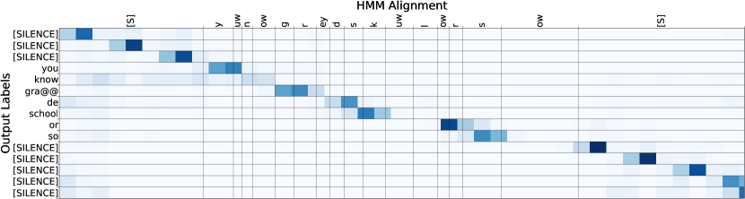
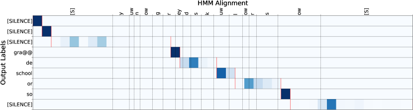
Fig. 4: Top: Attention weights of the global attention model. Bottom: Segment boundaries and attention weights of the segmental model. We also show the reference HMM alignment.

We also looked at the segment boundaries of the recognized sequence. The segment boundaries together with the attention weights can be seen in Figure 4. We notice that the segment boundaries are very off and they often cover multiple labels which explains the high deletion errors from Table 1. This observation is consistent over many other examples as well. We also make the same observations when we train the segmental model in contrast to importing the global attention model parameters.

To summarize: the label model yields good scores even for bad segment boundaries. This is probably due to the attention mechanism. This demonstrates that we need some sort of length model to get better segment boundaries.

4.2 Length model comparison

Table 3: Comparing different length models, with optional length normalization. Segmental search; models with silence.

Length model	Length norm.l	WER (%)				SE (%)
		S	D	I	$\Sigma$
None	No	$5.3$	$29.7$	$0.4$	$35.4$	$0.0$
	Yes	$6.4$	$17.2$	$1.7$	$25.3$	$0.4$
Static	No	$11.9$	$18.9$	$3.8$	$34.5$	$0.0$
	Yes	$10.2$	$16.3$	$5.1$	$31.7$	$0.0$
Neural	No	$9.0$	$6.2$	$1.9$	17.1 $\mathbf{17.1}$	$0.0$
	Yes	$9.1$	$5.9$	$2.0$	17.0 $\mathbf{17.0}$	$0.0$

In all following experiments, we always train the segmental model and do not import weights.

We compare our different length models and length normalization in Table 3. As expected, without any length model, the length normalization improves the performance. For the other length models, we use scale $\alpha=1$. We notice that the simple static length model yields even worse results than no length model. We analyze that in the following subsection and a tuned $\alpha$ will improve that. Overall, the neural length model yields the best results, where the length normalization has a negligible effect. In better segmental models with neural length model as presented later (e.g. Table 10), length normalization was hurtful and we did not use it. To conclude, length normalization is only needed without or with a weak length model.

4.3 Failures with static length model

Table 4: Segmental model scores using static length model: Label scores $\log p(a_{s}|...)$ and static length model $\log p(t_{s}|...)$.

Labels Label model scores Length model scores Ground-truth Recognized Ground-truth Recognized [Silence] $-0.11$ $-0.11$ $-1.00$ $-1.00$ [Silence] $-0.10$ $-0.10$ $-1.00$ $-1.00$ parti@@ $-0.10$ $-0.08$ $-1.47$ $-0.84$ cu@@ $-0.05$ $-0.04$ $-0.88$ $-0.88$ lar@@ $-0.06$ $-1.18$ $-1.57$ $-0.79$ ly $-0.05$ $-0.14$ $-1.16$ $-1.02$ if $-0.02$ (Deletion) $-1.59$ (Deletion) you’re $-0.61$ $-1.60$ h@@ $-0.27$ $-0.54$ $-0.81$ $-1.40$ un@@ $-0.06$ $-0.31$ $-0.89$ $-0.89$ g@@ $-0.01$ $-0.20$ $-1.67$ $-0.67$ ry $-0.03$ $-0.05$ $-1.03$ $-1.03$ … $\Sigma$ $-1.75$ $-2.90$ $-17.85$ $-10.52$

We want to better understand why the static length model fails and whether it fails for similar reasons as without any length model. We again look into the model scores for an example sequence in Table 4. Now we notice a new problem: The length model scores dominate much over the label scores. The label model scores of the ground-truth sequence is actually better than for the recognized sequence. However, the length model dominates and prefers some incorrect segment boundaries.

Table 5: Static length model scales ($\alpha$)

Length model scale	$0.0$	$0.01$	$0.1$	$0.3$	$1.0$
WER (%)	$25.3$	$23.9$	$\mathbf{21.8}$	$24.9$	$31.7$

To overcome this, we test different length model scales $\alpha$ in Table 5, to transition from no length model to the static length model. We see that we can still improve over the cases $\alpha=0$ or $\alpha=1$ but we are still behind the global attention model. To summarize: A weak length model also leads to suboptimal results. Thus we will focus now on the segmental model with neural length model.

4.4 Silence variants

Table 6: Comparing silence variants.

Model Silence variant WER (%) SE (%) S D I $\Sigma$ Global None $9.2$ $3.3$ $2.2$ $14.8$ $0.7$ No split $9.5$ $3.4$ $2.1$ $15.0$ $0.6$ Split $9.3$ $4.6$ $2.0$ $15.9$ $1.0$ Segmental None $8.7$ $3.5$ $1.9$ 14.1 $\mathbf{14.1}$ $0.0$ Split $9.0$ $6.2$ $1.9$ $17.1$ $0.0$

We compare the standard global-attention case of not having silence vs. having silence, either being split up into multiple segments in case they are too long, or not split up. The information on silence is extracted from our HMM alignment. The results are in Table 6. The variant without silence is better in all cases. Without silence, now the segmental attention model performs even better than the global attention model. We think that in principle it should be possible to improve the variant with silence and we have some ongoing work on this.

4.5 Search comparison

Table 7: Search comparison of simple search vs. segmental search, using segmental models with silence or without. *Not directly comparable because of CPU vs. GPU.

Variant	Simple search			Segmental search
	WER	SE	Time	WER	SE	Time
	(%)	(%)	(h)	(%)	(%)	(h)
W/o sil.	$15.0$	$0.8$	$0.1$*	$14.1$	$0.0$	$19.5$*
W/ sil.	$16.4$	$2.4$	$0.1$*	$17.1$	$0.0$	$11.6$*

Results of our two search implementations as described in Section 3.5 are collected in Table 7, comparing the same segmental model. Without silence, we get better performance with the segmental search. With silence, the result is unexpected. We can see that segmental search even has less search errors, so it looks like the model is worse but this needs further investigation, as also already mentioned in the last subsection. Segmental search is slower than simple search, although the numbers are not directly comparable due to CPU vs. GPU. Compared to the global attention model, for the segmental search, the computational complexity increases by a constant factor by the maximum segment length $\delta_{\text{max}}$, but the attention computation complexity decreases from $T\cdot S$ to $\delta_{\text{max}}\cdot S$, which dominates once $T$ becomes big.

4.6 State vector type

Table 8: Testing state vector dependency on $c_{1}^{s-1}$. Segmental model uses segmental search, neural length model.

Model	$c_{1}^{s-1}$ dependency	WER (%)	SE (%)
Global	Yes	15.3	0.5
	No	16.8	0.5
Segmental	Yes	14.5	0.0
	No	14.9	0.0

As described in Section 3.1, we have two variants of the state vector, either with dependency on $c_{1}^{s-1}$ or without. Results are in Table 8. As expected, the global attention model benefits a lot by having this dependency, as it can use it to better guide where to attend next. The difference is much smaller for the segmental model, as the attention is anyway only on the segment. However, it still slightly benefits from having the dependency.

4.7 Generalization on longer sequences

Table 9: Test generalization on longer sequences, concatenating $C$ consecutive sequences in the Hub5’00 corpora.

$C$ Seq. length (secs) WER (%) mean $\pm$ std min-max Global Segmental w/o sil. w/o sil. w/ sil. $1$ $\phantom{0}2.91\pm\phantom{0}2.57$ $0.08-\phantom{0}15.51$ $14.8$ $15.0$ $16.5$ $2$ $\phantom{0}8.10\pm\phantom{0}5.19$ $0.27-\phantom{0}63.97$ $15.1$ $15.7$ $17.6$ $4$ $18.28\pm\phantom{0}9.64$ $0.27-100.46$ $16.8$ $16.9$ $17.6$ $10$ $46.65\pm 22.52$ $0.33-198.10$ $33.9$ $19.3$ $18.6$ $20$ $87.41\pm 44.83$ $0.89-282.78$ $72.8$ $22.2$ $19.3$

We investigate performance on longer sequences than seen during training by simply concatenating $C$ consecutive sequences during recognition. We compare the global attention model to the segmental attention model and collect results in Table 9. The segmental model generalizes much better than global attention model. We also observe that the segmental model with explicit silence generalizes slightly better than without explicit silence. We believe that segmental models would generalize even better to very long sequences if they would have seen some sentence concatenation in training. Then, they should even improve the WER the longer the sequence becomes due to more context, as has been seen for language modeling [57, 6].

4.8 Overall comparison

Table 10: Overall comparison, comparing global attention models, transducers and segmental models from the literature and our final best models, different number of epochs (#Ep), seg. model uses length model scales 1.0 or 0.7.

Work Model Label #Ep LM WER (%) Type # $\text{Hub}5^{00}$ $\text{Hub}5^{01}$ $\text{RT}^{03}$ SWB CH $\Sigma$ SWB 2P3 2P4 $\Sigma$ SWB FSH $\Sigma$ [58] Gl.Att. BPE 534 $33$ no $14.6$ $14.0$ $16.8$ [49] Transd. BPE 1k $25$ no $9.4$ $18.7$ $14.1$ $14.1$ $16.7$ $50$ $8.7$ $18.3$ $13.5$ $13.3$ $15.6$ [59] Transd. Phon. 88 $100$ yes $11.2$ $11.2$ [60] Gl.Att. BPE 600 $\phantom{0}70$ no $6.7$ $13.0$ $9.9$ $7.1$ $9.2$ $13.7$ $10.1$ $15.7$ $9.1$ $12.5$ yes $5.5$ $11.2$ $8.4$ $6.1$ $7.7$ $11.4$ $8.5$ $12.6$ $7.0$ $9.9$ Ours Gl.Att. BPE 1k $\phantom{0}25$ no $9.1$ $20.4$ $14.8$ $10.4$ $13.1$ $18.6$ $14.2$ $20.4$ $12.9$ $16.8$ Seg./1.0 $9.3$ $19.0$ $14.2$ $10.3$ $13.1$ $18.1$ $14.0$ $19.9$ $12.8$ $16.5$ Seg./0.7 $9.2$ $19.0$ $14.1$ $10.3$ $12.9$ $18.0$ $13.9$ $19.8$ $12.6$ $16.4$ Seg./0.7 $50$ $8.8$ $18.5$ 13.7 $\mathbf{13.7}$ $10.0$ $12.4$ $17.4$ 13.4 $\mathbf{13.4}$ $19.4$ $12.4$ 16.0 $\mathbf{16.0}$

We collect our final results comparing our best global-attention model to our best segmental-attention model and other results from the literature in Table 10. Our segmental-attention model still uses an LSTM acoustic model, no external language model yet, and is not trained as long as other results which explains the gap to some other work from the literature. We see that segmental-attention overall performs slightly better than global-attention.

5 Conclusions

We introduced a novel type of segmental-attention models derived from the global-attention models. Our investigation of the modeling of the segment boundaries demonstrates and explains why a good length model is important for such models: the label model on its own still yields good scores even for bad segment boundaries. This can be explained due to the flexibility of attention but similar observations has also been made for other segmental models [40, 41]. This is in contrast to the experience of HMMs were the time-distortion penalties are less important.

In the end, our final segmental-attention model improves over the global-attention model, while at the same time satisfies all our motivations, namely it is monotonic, allows for online-streaming, potentially more efficient (at least the neural model, the search is currently slower but this is just for technical implementation reasons and can be improved), and it generalizes much better to long sequences. We think the segmental model can still be improved by not using $[{t_{s-1}+1},{t_{s}}]$ as the attention window but instead some fixed-size window where $t_{s}$ is the center position.

When looking at the equivalence of transducer and segmental models [47], we note that the main difference of our segmental model to common transducer models is the use of attention on the segment, while otherwise both models are conceptually similar.

6 Acknowledgements

This work was partially supported by NeuroSys which, as part of the initiative “Clusters4Future”, is funded by the Federal Ministry of Education and Research BMBF (03ZU1106DA); a Google Focused Award. The work reflects only the authors’ views and none of the funding parties is responsible for any use that may be made of the information it contains.

References

- [1] Dzmitry Bahdanau, Kyunghyun Cho, and Yoshua Bengio, “Neural machine translation by jointly learning to align and translate,” in 3rd International Conference on Learning Representations, ICLR 2015, San Diego, CA, USA, May 7-9, 2015, Conference Track Proceedings, Yoshua Bengio and Yann LeCun, Eds., 2015.
- [2] Jan K Chorowski, Dzmitry Bahdanau, Dmitriy Serdyuk, Kyunghyun Cho, and Yoshua Bengio, “Attention-based models for speech recognition,” in Advances in neural information processing systems, 2015, pp. 577–585.
- [3] William Chan, Navdeep Jaitly, Quoc V. Le, and Oriol Vinyals, “Listen, attend and spell: A neural network for large vocabulary conversational speech recognition,” in ICASSP, 2016.
- [4] Albert Zeyer, Kazuki Irie, Ralf Schlüter, and Hermann Ney, “Improved training of end-to-end attention models for speech recognition,” in Interspeech, Hyderabad, India, Sept. 2018.
- [5] Daniel S Park, William Chan, Yu Zhang, Chung-Cheng Chiu, Barret Zoph, Ekin D Cubuk, and Quoc V Le, “SpecAugment: A simple data augmentation method for automatic speech recognition,” in Proc. Interspeech 2019, 2019, pp. 2613–2617.
- [6] Zoltán Tüske, George Saon, Kartik Audhkhasi, and Brian Kingsbury, “Single headed attention based sequence-to-sequence model for state-of-the-art results on Switchboard,” in Proc. Interspeech 2020, 2020, pp. 551–555.
- [7] Jan Rosendahl, Viet Anh Khoa Tran, Weiyue Wang, and Hermann Ney, “Analysis of positional encodings for neural machine translation,” in IWSLT, Hong Kong, China, Nov. 2019.
- [8] Arun Narayanan, Rohit Prabhavalkar, Chung-Cheng Chiu, David Rybach, Tara N Sainath, and Trevor Strohman, “Recognizing long-form speech using streaming end-to-end models,” in ASRU, 2019.
- [9] Chung-Cheng Chiu, Wei Han, Yu Zhang, Ruoming Pang, Sergey Kishchenko, Patrick Nguyen, Arun Narayanan, Hank Liao, Shuyuan Zhang, Anjuli Kannan, Rohit Prabhavalkar, Zhifeng Chen, Tara N. Sainath, and Yonghui Wu, “A comparison of end-to-end models for long-form speech recognition,” in ASRU, 2019, pp. 889–896.
- [10] Chung-Cheng Chiu and Colin Raffel, “Monotonic chunkwise attention,” in Proceedings of the International Conference on Learning Representations (ICLR), 2018.
- [11] Ruchao Fan, Pan Zhou, Wei Chen, Jia Jia, and Gang Liu, “An online attention-based model for speech recognition,” in Interspeech, 2019.
- [12] Naveen Arivazhagan, Colin Cherry, Wolfgang Macherey, Chung-Cheng Chiu, Semih Yavuz, Ruoming Pang, Wei Li, and Colin Raffel, “Monotonic infinite lookback attention for simultaneous machine translation,” Preprint arXiv:1906.05218, 2019.
- [13] Dzmitry Bahdanau, Jan Chorowski, Dmitriy Serdyuk, Philemon Brakel, and Yoshua Bengio, “End-to-end attention-based large vocabulary speech recognition,” in 2016 IEEE international conference on acoustics, speech and signal processing (ICASSP). IEEE, 2016, pp. 4945–4949.
- [14] Thang Luong, Hieu Pham, and Christopher D. Manning, “Effective approaches to attention-based neural machine translation,” in Proceedings of the 2015 Conference on Empirical Methods in Natural Language Processing, Lisbon, Portugal, Sept. 2015, pp. 1412–1421, Association for Computational Linguistics.
- [15] Andros Tjandra, Sakriani Sakti, and Satoshi Nakamura, “Local monotonic attention mechanism for end-to-end speech and language processing,” in IJCNLP, 2017, vol. 1, pp. 431–440.
- [16] Shucong Zhang, Erfan Loweimi, Peter Bell, and Steve Renals, “Windowed attention mechanisms for speech recognition,” in Proc. IEEE Int. Conf. on Acoustics, Speech and Signal Processing (ICASSP). IEEE, Apr. 2019, pp. 7100–7104.
- [17] Navdeep Jaitly, Quoc V Le, Oriol Vinyals, Ilya Sutskever, David Sussillo, and Samy Bengio, “An online sequence-to-sequence model using partial conditioning,” in Advances in Neural Information Processing Systems, 2016, pp. 5067–5075.
- [18] Colin Raffel, Thang Luong, Peter J Liu, Ron J Weiss, and Douglas Eck, “Online and linear-time attention by enforcing monotonic alignments,” in Proceedings of the 34th International Conference on Machine Learning. 06–11 Aug 2017, Proceedings of Machine Learning Research, pp. 2837–2846, PMLR.
- [19] Andre Merboldt, Albert Zeyer, Ralf Schlüter, and Hermann Ney, “An analysis of local monotonic attention variants,” in Interspeech, Graz, Austria, Sept. 2019, pp. 1398–1402.
- [20] Roger Hsiao, Dogan Can, Tim Ng, Ruchir Travadi, and Arnab Ghoshal, “Online automatic speech recognition with listen, attend and spell model,” IEEE Signal Processing Letters, vol. 27, pp. 1889–1893, 2020, arXiv:2008.05514 [cs, eess].
- [21] Alex Graves, “Generating sequences with recurrent neural networks,” Preprint arXiv:1308.0850, 2013.
- [22] Junfeng Hou, Shiliang Zhang, and Lirong Dai, “Gaussian prediction based attention for online end-to-end speech recognition,” in Proc. Interspeech, Aug. 2017, pp. 3692–3696.
- [23] Jan Chorowski, Dzmitry Bahdanau, Kyunghyun Cho, and Yoshua Bengio, “End-to-end continuous speech recognition using attention-based recurrent NN: first results,” Preprint arXiv:1412.1602, 2014.
- [24] Alex Graves, Santiago Fernández, Faustino Gomez, and Jürgen Schmidhuber, “Connectionist temporal classification: labelling unsegmented sequence data with recurrent neural networks,” in Proceedings of the 23rd international conference on Machine learning. ACM, 2006, pp. 369–376.
- [25] Alex Graves, “Sequence transduction with recurrent neural networks,” Preprint arXiv:1211.3711, 2012.
- [26] Shinji Watanabe, Takaaki Hori, Suyoun Kim, John R Hershey, and Tomoki Hayashi, “Hybrid CTC/attention architecture for end-to-end speech recognition,” IEEE Journal of Selected Topics in Signal Processing, vol. 11, no. 8, pp. 1240–1253, Oct. 2017.
- [27] Takaaki Hori, Shinji Watanabe, and John R Hershey, “Joint CTC/attention decoding for end-to-end speech recognition,” in Proceedings of the 55th Annual Meeting of the Association for Computational Linguistics (Volume 1: Long Papers), 2017, pp. 518–529.
- [28] Suyoun Kim, Takaaki Hori, and Shinji Watanabe, “Joint CTC-attention based end-to-end speech recognition using multi-task learning,” in 2017 IEEE international conference on acoustics, speech and signal processing (ICASSP). IEEE, 2017, pp. 4835–4839.
- [29] Niko Moritz, Takaaki Hori, and Jonathan Le Roux, “Triggered attention for end-to-end speech recognition,” in ICASSP 2019-2019 IEEE International Conference on Acoustics, Speech and Signal Processing (ICASSP). IEEE, May 2019, pp. 5666–5670.
- [30] Niko Moritz, Takaaki Hori, and Jonathan Le Roux, “Streaming end-to-end speech recognition with joint CTC-attention based models,” in ASRU, Dec. 2019, pp. 936–943.
- [31] Haoran Miao, Gaofeng Cheng, Pengyuan Zhang, Ta Li, and Yonghong Yan, “Online hybrid CTC/attention architecture for end-to-end speech recognition,” in Interspeech, 2019, pp. 2623–2627.
- [32] Tara Sainath, Ruoming Pang, David Rybach, Yanzhang (Ryan) He, Rohit Prabhavalkar, Wei Li, Mirkó Visontai, Qiao Liang, Trevor Strohman, Yonghui Wu, Ian McGraw, and Chung-Cheng Chiu, “Two-pass end-to-end speech recognition,” in Interspeech, 2019.
- [33] Tara N. Sainath, Yanzhang He, Bo Li, Arun Narayanan, Ruoming Pang, Antoine Bruguier, Shuo-yiin Chang, Wei Li, Raziel Alvarez, Zhifeng Chen, Chung-Cheng Chiu, David Garcia, Alex Gruenstein, Ke Hu, Anjuli Kannan, Qiao Liang, Ian McGraw, Cal Peyser, Rohit Prabhavalkar, Golan Pundak, David Rybach, Yuan Shangguan, Yash Sheth, Trevor Strohman, Mirkó Visontai, Yonghui Wu, Yu Zhang, and Ding Zhao, “A streaming on-device end-to-end model surpassing server-side conventional model quality and latency,” in ICASSP 2020 - 2020 IEEE International Conference on Acoustics, Speech and Signal Processing (ICASSP), 2020, pp. 6059–6063.
- [34] Mari Ostendorf, Vassilios V Digalakis, and Owen A Kimball, “From HMM’s to segment models: A unified view of stochastic modeling for speech recognition,” IEEE Transactions on speech and audio processing, vol. 4, no. 5, pp. 360–378, 1996.
- [35] Lingpeng Kong, Chris Dyer, and Noah A Smith, “Segmental recurrent neural networks,” in ICLR, 2016.
- [36] Liang Lu, Lingpeng Kong, Chris Dyer, Noah A Smith, and Steve Renals, “Segmental recurrent neural networks for end-to-end speech recognition,” in Interspeech, 2016, pp. 385–389.
- [37] Lei Yu, Jan Buys, and Phil Blunsom, “Online segment to segment neural transduction,” in Proceedings of the 2016 Conference on Empirical Methods in Natural Language Processing. 2016, pp. 1307–1316, Association for Computational Linguistics.
- [38] Lei Yu, Phil Blunsom, Chris Dyer, Edward Grefenstette, and Tomas Kocisky, “The neural noisy channel,” in ICLR 2017, 2017.
- [39] Patrick Doetsch, Mirko Hannemann, Ralf Schlueter, and Hermann Ney, “Inverted alignments for end-to-end automatic speech recognition,” IEEE Journal of Selected Topics in Signal Processing, vol. 11, no. 8, pp. 1265–1273, Dec. 2017.
- [40] Eugen Beck, Mirko Hannemann, Patrick Doetsch, Ralf Schlüter, and Hermann Ney, “Segmental encoder-decoder models for large vocabulary automatic speech recognition,” in Interspeech, Hyderabad, India, Sept. 2018.
- [41] Eugen Beck, Albert Zeyer, Patrick Doetsch, André Merboldt, Ralf Schlüter, and Hermann Ney, “Sequence modeling and alignment for LVCSR-systems,” in ITG Conference on Speech Communication, Oldenburg, Oct. 2018.
- [42] Weiyue Wang, Tamer Alkhouli, Derui Zhu, and Hermann Ney, “Hybrid neural network alignment and lexicon model in direct HMM for statistical machine translation,” in ACL, Vancouver, Canada, Aug. 2017, pp. 125–131.
- [43] Weiyue Wang, Derui Zhu, Tamer Alkhouli, Zixuan Gan, and Hermann Ney, “Neural hidden Markov model for machine translation,” in ACL, Melbourne, Australia, July 2018, pp. 377–382.
- [44] Tamer Alkhouli, Gabriel Bretschner, Jan-Thorsten Peter, Mohammed Hethnawi, Andreas Guta, and Hermann Ney, “Alignment-based neural machine translation,” in ACL, Berlin, Germany, Aug. 2016, pp. 54–65.
- [45] Tamer Alkhouli, Alignment-Based Neural Networks for Machine Translation, Ph.D. thesis, RWTH Aachen University, Computer Science Department, RWTH Aachen University, Aachen, Germany, July 2020.
- [46] Albert Zeyer, Ralf Schlüter, and Hermann Ney, “A study of latent monotonic attention variants,” Preprint arXiv:2103.16710, Mar. 2021.
- [47] Wei Zhou, Albert Zeyer, André Merboldt, Ralf Schlüter, and Hermann Ney, “Equivalence of segmental and neural transducer modeling: A proof of concept,” in Interspeech, Aug. 2021, pp. 2891–2895, [slides].
- [48] Albert Zeyer, Parnia Bahar, Kazuki Irie, Ralf Schlüter, and Hermann Ney, “A comparison of Transformer and LSTM encoder decoder models for ASR,” in IEEE Automatic Speech Recognition and Understanding Workshop, Sentosa, Singapore, Dec. 2019, pp. 8–15.
- [49] Albert Zeyer, André Merboldt, Ralf Schlüter, and Hermann Ney, “A new training pipeline for an improved neural transducer,” in Interspeech, http://www.interspeech2020.org/, Oct. 2020, [slides].
- [50] Sepp Hochreiter and Jürgen Schmidhuber, “Long short-term memory,” Neural computation, vol. 9, no. 8, pp. 1735–1780, 1997.
- [51] Hasim Sak, Matt Shannon, Kanishka Rao, and Françoise Beaufays, “Recurrent neural aligner: An encoder-decoder neural network model for sequence to sequence mapping,” in Proc. of Interspeech, 2017.
- [52] Kenton Murray and David Chiang, “Correcting length bias in neural machine translation,” in Proc. WMT, Belgium, Brussels, Oct. 2018, pp. 212–223.
- [53] John J Godfrey, Edward C Holliman, and Jane McDaniel, “Switchboard: Telephone speech corpus for research and development,” in ICASSP, 1992, pp. 517–520.
- [54] Rico Sennrich, Barry Haddow, and Alexandra Birch, “Neural machine translation of rare words with subword units,” in ACL, Berlin, Germany, August 2016, pp. 1715–1725.
- [55] Albert Zeyer, Tamer Alkhouli, and Hermann Ney, “Returnn as a generic flexible neural toolkit with application to translation and speech recognition,” in Annual Meeting of the Assoc. for Computational Linguistics, Melbourne, Australia, July 2018.
- [56] David Rybach, Stefan Hahn, Patrick Lehnen, David Nolden, Martin Sundermeyer, Zoltán Tüske, Simon Wiesler, Ralf Schlüter, and Hermann Ney, “Rasr - the rwth aachen university open source speech recognition toolkit,” in IEEE Automatic Speech Recognition and Understanding Workshop, Waikoloa, HI, USA, Dec. 2011.
- [57] Kazuki Irie, Albert Zeyer, Ralf Schlüter, and Hermann Ney, “Training language models for long-span cross-sentence evaluation,” in IEEE Automatic Speech Recognition and Understanding Workshop, Sentosa, Singapore, Dec. 2019, pp. 419–426.
- [58] Mohammad Zeineldeen, Aleksandr Glushko, Wilfried Michel, Albert Zeyer, Ralf Schlüter, and Hermann Ney, “Investigating methods to improve language model integration for attention-based encoder-decoder ASR models,” in Interspeech, Aug. 2021, [slides], [video].
- [59] Wei Zhou, Simon Berger, Ralf Schlüter, and Hermann Ney, “Phoneme based neural transducer for large vocabulary speech recognition,” in IEEE International Conference on Acoustics, Speech, and Signal Processing, June 2021, To appear.
- [60] Zoltán Tüske, George Saon, and Brian Kingsbury, “On the limit of English conversational speech recognition,” in Proc. Interspeech 2021, 2021, pp. 2062–2066.