Deterministic and stochastic sampling of two coupled Kerr parametric oscillators

Abstract

The vision of building computational hardware for problem optimization has spurred large efforts in the physics community. In particular, networks of Kerr parametric oscillators (KPOs) are envisioned as simulators for finding the ground states of Ising Hamiltonians. It was shown, however, that KPO networks can feature large numbers of unexpected solutions that are difficult to sample with the existing deterministic (i.e., adiabatic) protocols. In this work, we experimentally realize a system of two classical coupled KPOs, and we find good agreement with the predicted mapping to Ising states. We then introduce a protocol based on stochastic sampling of the system, and we show how the resulting probability distribution can be used to identify the ground state of the corresponding Ising Hamiltonian. This method is akin to a Monte Carlo sampling of multiple out-of-equilibrium stationary states and is less prone to become trapped in local minima than deterministic protocols.

The Kerr parametric oscillator (KPO) is a nonlinear system whose potential energy is modulated at a frequency $f_{p}$ close to twice its resonance frequency, $f_{p}\approx 2f_{0}$ Ryvkine and Dykman (2006); Mahboob and Yamaguchi (2008); Wilson et al. (2010); Eichler et al. (2011); Leuch et al. (2016); Gieseler et al. (2012); Lin et al. (2014); Puri et al. (2017a); Eichler et al. (2018); Nosan et al. (2019); Frimmer et al. (2019); Grimm et al. (2020); Wang et al. (2019); Puri et al. (2019); Miller et al. (2019); Yamaji et al. (2022). When the modulation depth $\lambda$ exceeds a threshold $\lambda_{\mathrm{th}}$, the system features two stationary oscillation solutions. The solutions have a frequency $f_{p}/2$, an amplitude $X$ determined by $\lambda$ relative to the Kerr nonlinearity, and phases that differ by $\pi$. These ‘phase states’ can be mapped to the two states $\sigma\in\{-1,1\}$ of an Ising spin. Building on that analogy, it was proposed that networks of KPOs can be utilized to simulate the ground state of coupled spin ensembles, as captured by the Ising model Hamiltonian Ising (1925):

$$H_{\mathrm{Ising}}=-\sum_{i,j}K_{i,j}\sigma_{i}\sigma_{j}\,,$$

where $K_{i,j}$ is the coupling coefficient between two spins with states $\sigma_{i,j}$. Interestingly, finding this ground state is equivalent to many computational problems that are nearly intractable with conventional computers Mohseni et al. (2022), such as the number partitioning problem Nigg et al. (2017), the MAX-CUT problem Inagaki et al. (2016a); Goto et al. (2019), and the famous traveling salesman problem Lucas (2014).

Various physical implementations have been proposed or realized as “Ising solvers” Gottesman et al. (2001); Devoret and Schoelkopf (2013); Mahboob et al. (2016); Inagaki et al. (2016b); Goto (2016); Puri et al. (2019); Bello et al. (2019); Okawachi et al. (2020). A well known example is the Coherent Ising Machine, a network of degenerate optical parametric oscillators (DOPOs) that are coupled through a programmable electronic feedback element Wang et al. (2013); Inagaki et al. (2016a); Mahboob et al. (2016); Yamamoto et al. (2017); Yamamura et al. (2017); Bello et al. (2019) (note that DOPOs differ from KPOs in that their amplitude is not determined by their Kerr nonlinearity but rather by two-photon loss). The feedback breaks the energy conservation of the network and imparts dissipative coupling (mutual damping) between the oscillators. As a consequence, different network configurations corresponding to different Ising solutions become stable at different driving thresholds. The optimal solution is assumed to possess the lowest threshold and therefore to appear as the solution when driving the network.

A different line of investigation focuses on energy-conserving, bilinear coupling between KPOs Goto (2016); Puri et al. (2017b); Nigg et al. (2017); Goto et al. (2018); Dykman et al. (2018); Rota et al. (2019); Heugel et al. (2022a). In this works, the coupled oscillator solutions can be approximated as decoupled normal modes with split resonance frequencies. In contrast to the case of dissipative coupling, the lowest threshold that is encountered when ramping up the driving strength depends here on the detuning $\Delta$ between the external drive and the resonance frequency. This control parameter opens up the possibility for specific protocols to find different solutions Goto (2016); Puri et al. (2017b); Nigg et al. (2017). It was experimentally demonstrated, however, that the combination of nonlinearities and strong bilinear coupling can give rise to a rich solution space beyond that of a simple Ising model Heugel et al. (2022a). Careful validation and testing of small systems is therefore important before larger networks can be understood and operated correctly.

In this paper, we experimentally test the validity of the Ising analogy for a system of two classical coupled KPOs. In a first step, we apply an adiabatic ramping protocol to find one particular solution for each selected combination of $\Delta$ and $\lambda$ in a deterministic way. In a second step, we use strong force noise to explore the solution space of the system: this method is based on transitions between different stationary KPO solutions Dykman et al. (1998); Chan and Stambaugh (2007); Chan et al. (2008); Mahboob et al. (2014); Margiani et al. (2022), and it allows for the visualization of a probability distribution for all accessible states. Such “stochastic sampling” presents a way of quantifying the occupation probability of each solution, and thus selecting the optimal state. Surprisingly, we find that the oscillation state corresponding to the expected Ising ground state has not the highest but the lowest occupation probability over the entire parameter space. We reconcile this result with theory and predict how the method can be used for larger networks.

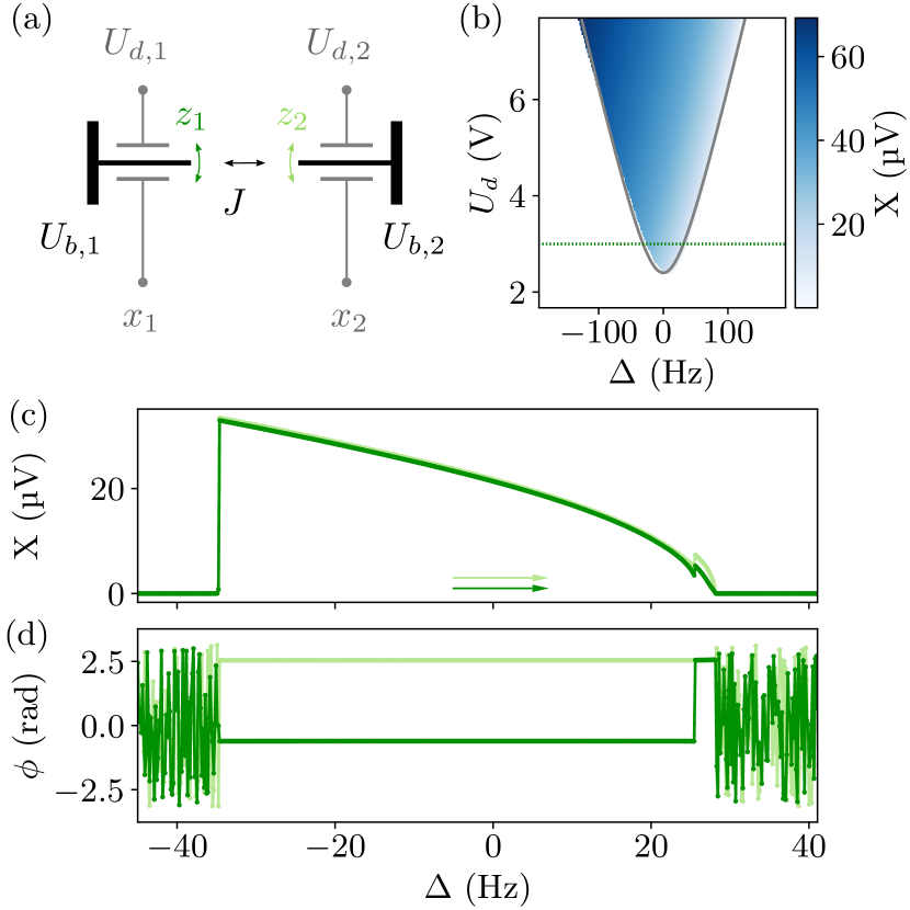
Figure 1: Device and basic characterization. (a) Simplified schematic of our setup: Two mechanical resonators are coupled with a strength $J$ via their common substrate. The devices are charged (and tuned) with bias voltages $U_{b,i}$ and driven by $U_{d,i}$. Their displacement $z_{i}$ capacitively translates into a voltage $x_{i}$ that is read out. (b) The Arnold tongue of a single KPO indicates the region in a space spanned by $\Delta$ and $U_{\mathrm{d}}\propto\lambda$ where the zero-amplitude state becomes unstable and the resonators respond with a finite amplitude $X$. The solid gray line indicates the theoretical threshold $U_{\mathrm{th}}$ (see Appendix A). (c) Amplitude and (d) phase of the two resonators in a frequency sweep from low to high frequencies (direction of arrows) with $U_{\mathrm{d}}=$3\text{\,}\mathrm{V}$$; cf. the green dashed line in (b). Close to $\Delta=$25\text{\,}\mathrm{Hz}$$, one of the KPOs (dark green) flips its phase while the other (bright green) remains in the same phase state. The system’s state changes from antisymmetric to symmetric at this point. Outside of the Arnold tongue, the phases are undefined. Note that for the opposite sweep direction, the state change does not occur. Instead, the system follows the symmetric state as long as it remains stable.

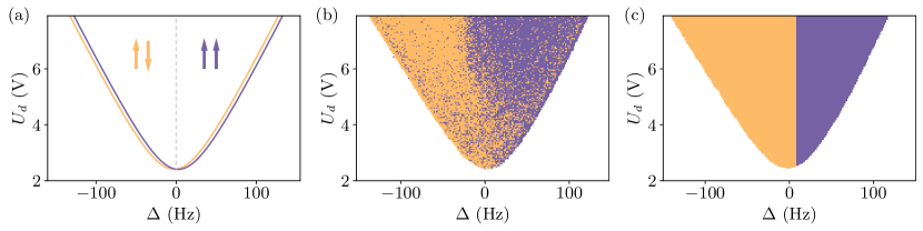
Figure 2: Deterministic sampling of the coupled system. (a) Schematic shapes (with exaggerated splitting) of the two overlapping Arnold tongues centered at $f_{A,S}=f_{0}\pm\Delta_{f}/2$. Each tongue has the boundaries $f_{\pm}^{2}=f_{A,S}^{2}\left(1\pm\sqrt{\frac{\lambda^{2}}{4}-\frac{1}{Q^{2}}}\right)$. The tongue for the antisymmetric and symmetric normal mode are shown in orange and purple, respectively. $\Delta=0$ is shown as a dashed grey line and arrows indicate the solution with the lowest threshold for positive and negative $\Delta$. (b) Measured response to a parametric drive initialized with fixed strength $U_{\mathrm{d}}$ and detuning $\Delta$. For each drive-frequency pair, the parametric drive was activated and the system was given approx. $400\text{\,}\mathrm{ms}$ to settle into a solution before the result was recorded with an integration time of $16\text{\,}\mathrm{ms}$. Afterwards, the drive was switched off for $400\text{\,}\mathrm{ms}$ before moving on to the next coordinate. Symmetric (purple) and antisymmetric (orange) solutions were identified by comparing the measured phases of the two KPOs, while the shape of the Arnold tongue was extracted from their amplitudes. (c) Measured response to a parametric drive initialized with detuning $\Delta$ and a strength that is slowly ramped upwards from $U_{\mathrm{d}}=0$ with no initial oscillation (white). The color coding is the same as in (b).

Our system comprises two microelectromechanical resonators (MEMS) made from highly-doped single-crystal silicon. Both resonators are fabricated on the same chip in a wafer-scale encapsulation process Yang et al. (2016), and they have the shape of double-ended tuning forks with branches $200\text{\,}\mathrm{\SIUnitSymbolMicro m}$ long and $6\text{\,}\mathrm{\SIUnitSymbolMicro m}$ thick; see Fig. 1(a) and Appendix A. They have resonance frequencies of roughly $f_{0}\approx$1.124\text{\,}\mathrm{MHz}$$ and quality factors of $Q\approx 13500$. Bias voltages $U_{b}$ can be used to fine-tune the resonator frequencies by a few $\mathrm{kHz}$ and induce negative Kerr-nonlinear coefficients of $\beta\approx$-63.2\text{\times}{10}^{17}\text{\,}{\mathrm{V}}^{-2}\text{\,}{\mathrm{s}}^{-2}$$ due to the nonlinear electrostatic forces between the biased tuning fork and the electrodes next to it Agarwal et al. (2008). Those electrodes capacitively transduce the motion into electrical signals that are measured with a Zurich Instruments HF2LI lock-in amplifier. The capacitive driving and measurement allows us to write effective equations of motion Nosan et al. (2019) as

$$\ddot{x}_{i}+\omega_{0}^{2}\left[1-\lambda\cos\left(2\pi f_{p}t\right)\right]x_{i}+\beta x_{i}^{3}+\gamma\dot{x}_{i}-Jx_{j}=U_{\xi,i}\,,$$

where $\omega_{0}/2\pi=f_{0}$, $\gamma=\frac{\omega_{0}}{Q}$, $x_{i}$ is the measured voltage signal of resonator $i$, $J$ quantifies the coupling to resonator $j$, and $U_{\xi,i}$ indicate uncorrelated white noise sources. The electrical tuning effect allows us to parametrically modulate (drive) the resonator potentials at frequency $f_{p}$ Margiani et al. (2022). The required oscillating driving voltage is $U_{\mathrm{d}}=\lambda U_{\mathrm{th}}^{0}Q/2$, where $U_{\mathrm{th}}^{0}\approx$2.4\text{\,}\mathrm{V}$$ is the measured parametric threshold voltage on resonance. As a function of detuning $\Delta=f_{p}/2-f_{0}$, the driving threshold for parametric oscillation, $U_{\mathrm{th}}$, is described by a so-called ‘Arnold tongue’, see Fig. 1(b). Outside the Arnold tongue, a resonator is stable at zero amplitude, while inside the tongue the zero-amplitude solution becomes unstable and the resonator oscillates at $f_{p}/2$ with a finite effective amplitude $X$ in one out of two possible phase states.

The resonators are mechanically coupled via their common substrate Miller et al. (2022). We calibrate the coupling strength from the normal-mode splitting and find $\Delta_{f}=$-2.6\pm 0.3\text{\,}\mathrm{Hz}$$, corresponding to a coupling coefficient $J=4\pi^{2}\Delta_{f}f_{0}=-$(113\pm 13.)\text{\times}{10}^{6}\text{\,}{\mathrm{Hz}}^{2}$$ between the two resonators; see Appendix A for details. Even though the coupling is weak, $|\Delta_{f}|\ll f_{0}/Q$, we can use a normal-mode basis of antisymmetric and symmetric oscillations to describe our system in the following.

When both resonators are operated as KPOs with a parametric drive voltage $U_{\mathrm{d}}>U_{\mathrm{th}}$, each of them selects one of its two phase states. The resonators can respond either in the same (symmetric) or in opposite (antisymmetric) phases. Which of those two solutions is preferred depends on the signs of $J$ and $\Delta$. In Figs. 1(c) and 1(d), we show the experimental results of sweeping the driving frequency from negative to positive $\Delta$ at a fixed $U_{\mathrm{d}}$. The system first rings up into the antisymmetric state at $\Delta=$-35\text{\,}\mathrm{Hz}$$ before it flips to a symmetric configuration close to $\Delta=$25\text{\,}\mathrm{Hz}$$.

The ordering observed in Figs. 1(c) and 1(d) reflects the fact that for $J<0$, the antisymmetric normal mode has a lower eigenfrequency than the symmetric mode. We can therefore expect to find separate normal-mode Arnold tongues for symmetric and antisymmetric oscillations with a splitting in frequency; see Fig. 2(a) Heugel et al. (2019, 2022a). This splitting has important consequences for the driven system: when the drive is suddenly activated at a specific detuning $\Delta$ above threshold, the KPOs should preferentially select the normal-mode oscillation state with the lowest threshold. We experimentally test this prediction in Fig. 2(b) by measuring the chosen state once for each pixel individually, and we find very good agreement with the schematic in Fig. 2(a). Note the narrow regions on the left and right boundaries where only one state can be activated. These regions are a direct confirmation of the normal-mode splitting.

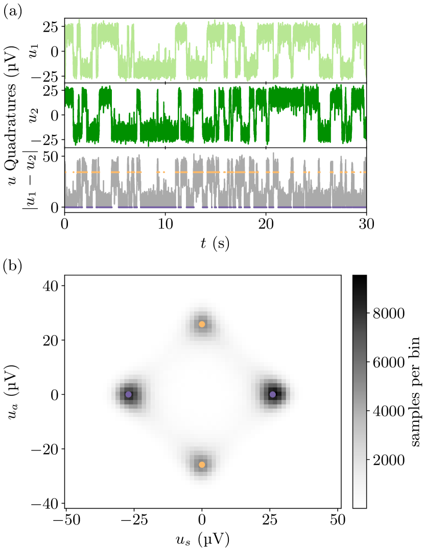
Figure 3: Stochastic sampling of the coupled system. (a) Extract from a measured sample path of both KPOs under the influence of applied force noise. Switches between the quasistable states are visible as jumps from $-$25\text{\,}\mathrm{mV}$$ to $+$25\text{\,}\mathrm{mV}$$ and vice versa. Only the $u$ quadratures and their difference are shown for simplicity. A high difference indicates that the system is in an antisymmetric state (orange dots), while differences close to zero correspond to a symmetric state (purple dots). (b) Representation of the entire sample path in a “super phase space” spanned by $u_{s}=(u_{1}+u_{2})/\sqrt{2}$ and $u_{a}=(u_{1}-u_{2})/\sqrt{2}$. Orange and purple dots mark the antisymmetric ($u_{s}\approx 0$) and symmetric ($u_{a}\approx 0$) phase state configurations, respectively. The graph also shows how switches mostly involve a change in symmetry from symmetric to antisymmetric or vice versa, while symmetry-preserving transitions through the origin of the plot are rare. We use $U_{\mathrm{d}}=$3\text{\,}\mathrm{V}$$ and $\Delta=0$. The total measurement time was $6\text{\,}\min$, measured with an integration time of $138\text{\,}\mathrm{\SIUnitSymbolMicro s}$ at 3597 samples per second.

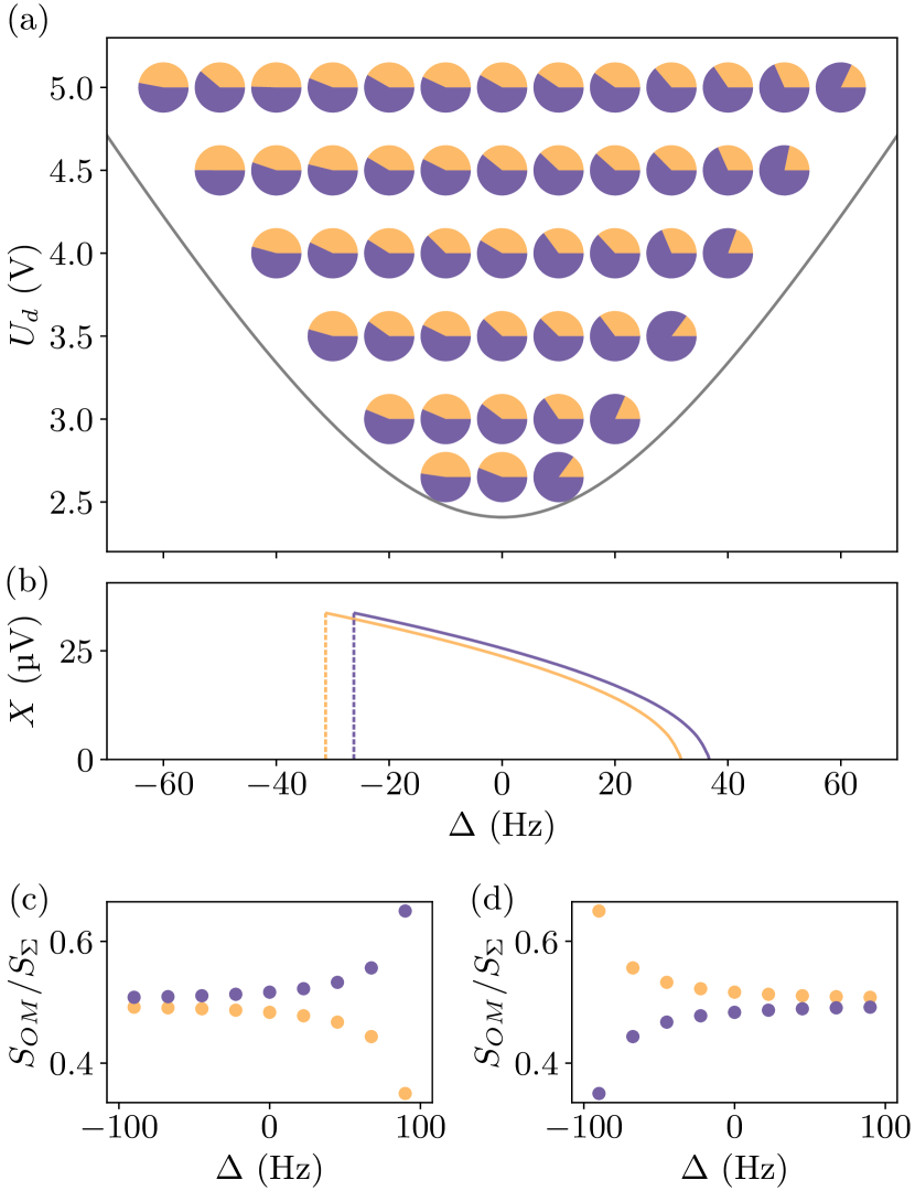
Figure 4: Relative occupation of solutions. (a) Cake diagrams show the relative time the system spent in the antisymmetric (orange) and symmetric (purple) solution, at a given detuning $\Delta$ and driving $U_{\mathrm{d}}$. The coupling coefficient in this measurement was $J=-$(96\pm 13.)\text{\times}{10}^{6}\text{\,}{\mathrm{Hz}}^{2}$$. The noise strength $U_{\xi}$ was varied in proportion with the response amplitude of the KPOs to keep the switching rate within reasonable bounds. As a consequence, only the qualitative result at each position is significant, i.e., which solution has the longer average dwell time. A gray line indicates the boundary of the Arnold tongue. See Appendix B for details. (b) Schematic shapes of antisymmetric (orange) and symmetric (purple) solutions as a function of detuning. The splitting is exaggerated for better visibility. (c) Normalised Onsager-Machlup action $S_{\mathrm{OM}}$ for switching away from antisymmetric (orange) and symmetric (purple) solutions. The results are normalised with the sum of the symmetric and antisymmetric values ($S_{\Sigma}$) and shown as a function of normalised detuning. A higher $S_{\mathrm{OM}}$ corresponds to a longer dwell time in a state (see Appendix C). The values are calculated for the experimental parameters with $\lambda=0.0004$, corresponding to $U_{\mathrm{d}}\approx$6.48\text{\,}\mathrm{V}$$. (d) Same calculation as in (c) but with the opposite sign of the nonlinearity, $\beta>0$.

Figure 2(a) offers a simple interpretation of several recent theory proposals for simulating the Ising ground state with KPO networks  Goto (2016); Puri et al. (2017b); Nigg et al. (2017). The proposals predict that for quasiadiabatic ramping of $U_{\mathrm{d}}$ with $\Delta<0$, the stable solution emerging beyond the lowest instability threshold corresponds to the correct Ising ground-state solution. As we see in Fig. 2(a), such a protocol can effectively be reduced to finding the normal mode with the lowest eigenfrequency in the case of two coupled KPOs. We confirm the protocol in Fig. 2(c). Our system rings up to symmetric and antisymmetric states for $\Delta>0$ and $\Delta<0$, respectively. As the Ising ground state we seek is the antiferromagnetic one, the latter presents the correct solution. Note that the protocol would still work for $J>0$, as both the Ising ground state and the normal-mode ordering would then be reversed. For strong coupling and larger networks, additional nonlinear effects can make the solution space more complex to map Heugel et al. (2022a). This will be the scope of future experiments.

The statistical spread of states in Fig. 2(b) can be understood from the competition between deterministic ordering due to the coupling term $J$ on the one hand, and stochastic (thermal) force noise on the other hand. When the drive is switched on suddenly, noise in a wide frequency range participates in this competition. Note, however, that the noise intensity is always finite, resulting in a finite statistical bias towards the solution preferred by the coupled system. Slow ramping of the drive additionally low-pass filters the noise and favors a deterministic ordering. This is why the outcome in Fig. 2(c) is neatly divided into two halves.

Instead of suppressing the noise, it can be interesting to enhance it in order to enable activated jumps between all states. In this way, we gain a “stochastic sampling” map of the solution space at particular values of $U_{\mathrm{d}}$ and $\Delta$, rather than just a single solution Heugel et al. (2022b). Activated escape involves a random walk from the initial state (first quasipotential well) over a quasienergy barrier, and a deterministic decay into the opposite state (second quasipotential well) Dykman and Krivoglaz (1979); Dykman et al. (1993). In analogy to a thermodynamic system, we naively expect that the optimal solution occupies the deepest quasipotential well and therefore has the longest average dwell time $\tau$ between switches Dykman et al. (2018); Margiani et al. (2022).

We test the stochastic sampling protocol in Fig. 3. White voltage noise with a standard deviation $U_{\xi,i}$ applied to each drive electrode enhances the force noise enough to cause activated jumps between the symmetric and antisymmetric solutions as a function of time; see Fig. 3(a) Margiani et al. (2022). Plotting such a data set as a function of the variables $u_{s}=(u_{1}+u_{2})/\sqrt{2}$ and $u_{a}=(u_{1}-u_{2})/\sqrt{2}$, where we define $x_{i}(t)=u_{i}\cos(\pi f_{\mathrm{p}}t)+v_{i}\sin(\pi f_{\mathrm{p}}t)$, allows us to identify symmetric and antisymmetric solutions, respectively, cf. Fig. 3(b).

We repeat the stochastic sampling for different values of $\Delta$ and $U_{\mathrm{d}}$, and we summarize the results in Fig. 4. The relative dwell times measured for the symmetric and antisymmetric states are shown in cake diagrams. Surprisingly, the driven out-of-equilibrium system favors the symmetric state in the entire range of parameters. This is in contrast to the behavior expected from the corresponding (equilibrium) Ising Hamiltonian $H_{\mathrm{Ising}}$, where the antisymmetric ground state would always have the highest occupation.

To investigate this enigma, we compare the switching paths that can carry the system from the symmetric to the antisymmetric state or vice versa. For small switching probabilities, the main contribution of the random walk is concentrated in a narrow channel in phase space Chan et al. (2008), such that we can approximate the total switching rate from the optimal switching path $\mathbf{Y}_{\rm min}$ for each transition (see Appendix C).

The theory results obtained for our device parameters agree with our experimental findings. As shown in Fig. 4(c), the results consistently predict longer dwell times for the symmetric configuration than for the antisymmetric one over the entire range of $\Delta$, meaning that the time required to escape the quasipotential well of the symmetric state is longer on average. The ordering of the dwell time coincides with that of the state amplitudes shown in Fig. 4(b). Interestingly, when repeating the calculations for a positive nonlinearity $\beta$, the result changes and the antisymmetric state is found to be more stable in general; see Fig. 4(d). Note that switching the sign of $\beta$ changes the ordering of the amplitudes of the normal modes in Fig. 4(b) as well. We conclude that for the system we study, the most stable state is always the one with the largest amplitude.

We can understand the experimental and theoretical results in a straightforward way. To switch from one normal mode to another, one of the participating resonators must switch to the opposite phase state, which can be achieved without energy transfer Roychowdhury (2015); Frimmer et al. (2019) but implies a momentum reversal. With all other parameters being approximately equal, a larger normal-mode oscillation amplitude corresponds to a larger momentum to be overcome by the stochastic process. For this reason, the system typically remains trapped for a longer time in the solution with the highest amplitude, as seen in Fig. 4.

Our experimental confirmation of Ising simulation protocols Goto (2016); Puri et al. (2017b); Nigg et al. (2017) is a first step towards understanding large systems. For $N>2$, the number of normal modes does not match the expected size of the Ising solution space, and it will be important to understand how the system evolves far beyond the parametric threshold as a function of detuning Heugel et al. (2022a) and in the presence of persistent beating between solutions Strinati et al. (2020). Mapping all solutions of a complex system can be difficult with deterministic drives due to hysteresis. Stochastic sampling, as demonstrated here, may be a way to overcome this limitation, providing a direct tomography of the solution space for a given parameter set. More generally, stochastic sampling or related experiments such as simulated annealing can be useful for understanding the analogy between an out-of-equilibrium nonlinear resonator network and thermodynamic systems. As we show in this work, the connection between the two paradigms can be counterintuitive.

Finally, we include a brief outlook on performing Ising simulation protocols with quantum-coherent systems. Quantum systems are predicted to be more efficient in finding the Ising ground state than the corresponding classical system Goto (2016), which makes them a valuable resource for solving optimization problems Mohseni et al. (2022). There, the competition between the timescales set by decoherence on the one hand and energy exchange between the KPOs on the other hand implies that strong coupling is a crucial requirement for quantum adiabatic evolution. However, the combination of strong coupling and nonlinearity was shown to impact the Ising solution space in surprising ways, calling for careful calibration Heugel et al. (2022a, b). For this reason, the development of quantum systems will benefit from methods such as stochastic sampling that allow visualizing the complete solution space.

Appendix A Devices and Basic Characterization

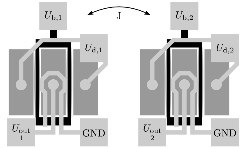
Figure 5: Schematic of the resonators. The oscillating tuning forks are drawn in black. Each fork is fixed at the top and polarised by applying a bias voltage to the $U_{\mathrm{b,i}}$ pads (light gray). The two branches of a single fork are then driven into opposite motion by a capacitive force exerted from a varying voltage on the dark grey electrodes next to the beams. Readout is performed by measuring the voltage on the center dark gray electrode relative to ground Agarwal et al. (2008). Connections and pads on top of the chip are shown in light gray. The two resonators are mechanically coupled via their common substrate.

Detailed schematics showing the two tuning-fork resonators and the electrodes for capacitive driving are shown in Fig. 5.

The resonators’ properties were extracted from fits to their driven response. Applying a small driving force to only one of the resonators allows us to extract the precise resonance frequency as well as the quality factor. The same measurement can give a clear indication of coupling between the resonators when looking at the response of the nondriven resonator, cf. Fig. 6. Due to the frequency-dependent driving amplitude and phase that the second resonator experiences, its amplitude response is narrower than usual and its phase changes by $180\text{\,}\mathrm{\SIUnitSymbolDegree}$ when crossing the resonance.

The parametric threshold was found by measuring a full Arnold tongue, whose tip (lowest point) corresponds to the effective threshold on resonance $U_{\mathrm{th}}^{0}$ while the outer shape is determined by

$$U_{\mathrm{th}}=\frac{U_{\mathrm{th}}^{0}Q}{2}\sqrt{4\left(\left(\frac{\omega^{2}}{\omega_{0}^{2}}-1\right)^{2}+\frac{1}{Q^{2}}\right)}\,,$$ (1)

cf. Fig. 1(b) Lifshitz and Cross (2009). Equation (1) is a reformulation of the formula for $f_{\pm}$ shown in the caption to Fig. 2(a). The parametric modulation depth is calibrated as $\lambda=\frac{2U_{d}}{QU_{\mathrm{th}}^{0}}$. The amplitudes in a single line above threshold can then be used to determine the Duffing nonlinearity factor by fitting the parametric frequency response amplitude:

$$|X(\omega)|=\Re\left(\sqrt{\frac{4\omega_{0}^{2}}{3\beta}(\pm i\sqrt{c}+b-1)}\right)\,,$$ (2)

where $\omega=\pi f_{p}$, $b=\frac{\omega^{2}}{\omega_{0}^{2}}$ and $c=\frac{-\lambda^{2}}{4}+\frac{\gamma^{2}\omega^{2}}{\omega_{0}^{4}}$, cf. Fig. 1(c). Finally, we extract the coupling strength from the data in Fig. 1(d). With the frequency difference $\Delta_{f}$ between the end of the antisymmetric response and the end of the symmetric response, the coupling coefficient can be calculated as $J=2\pi\Delta_{f}\omega_{0}$. The sign of the coupling then follows from the ordering of symmetric and antisymmetric responses. A comparable result can be extracted from the resonant amplitudes in Fig. 6. For $X_{\mathrm{d}}$ and $X_{\mathrm{n}}$ being the amplitudes at resonance of the driven and coupled, nondriven resonator respectively, we find $J=-\frac{X_{\mathrm{n}}}{X_{\mathrm{d}}}\frac{\omega_{0}^{2}}{Q}$.

Appendix B Stochastic Sampling

To test the stochastic sampling protocol as shown in Fig. 4, we measured a set of time traces for different frequencies $\Delta$ and parametric driving strengths $U_{\mathrm{d}}$. Each measured time trace is $360\text{\,}\mathrm{s}$ long with 3597 samples per second. We heuristically adjusted the standard deviation $\sigma_{\mathrm{\xi}}$ of the white noise $U_{\mathrm{\xi,i}}$ applied to the resonators together with the drive as $\sigma_{\mathrm{\xi}}\approx 4\times 10^{4}\times(1.57X-0.01)$ to reach a reasonable switching rate over the parameter range of the measurement.

In a first analysis step, each data point from a single KPO was assigned to one of the phase states labeled $0$ or $\pi$. In order to do so, we defined circles in phase space whose center point were the stable attractors and whose radii were $0.6$ times the state amplitude. A data point was assigned to a phase state when it was within the respective circle. If the data point was outside both circles, it was assigned to the same state as the previous data point. See Ref. Margiani et al. (2022) for details.

In a second step, we then compared the relative states of both KPOs, counting how often the two phase states are equal or opposite. The results of those polls are shown in the cake diagrams in Fig. 4. They give a qualitative estimate of which state the system prefers to be in.

Appendix C Onsager-Machlup Function

The switching process between stable oscillation states induced by weak-noise can be described analogously to noise-activated jumping over a barrier $W$ in equilibrium systems Stambaugh and Chan (2006); Hänggi et al. (1990). However, the barrier $W$ between two quasistable solutions of a driven system resides in a quasipotential structure in a rotating frame. The Onsager-Machlup formalism can be used to obtain an estimate for the barrier $W$ Lehmann et al. (2003); Coffey (2013). The Onsager-Machlup action is defined by:

$$S_{\rm OM}[\mathbf{Y}]=\int_{t_{i}}^{t_{f}}\frac{1}{4}\left(\dot{\mathbf{Y}}-\mathbf{f}(\mathbf{Y})\right)^{2}dt\,,$$ (3)

where $t_{i}$ ($t_{f}$) is the initial (final) time of the trajectory of the $N$ resonator system, $\mathbf{Y}(t)=(u_{1},v_{1},...,u_{N},v_{N})$, which obeys the equation of motion $\dot{\mathbf{Y}}=\mathbf{f}(\mathbf{Y})$. For the switching rate $\Gamma$ in the weak-noise limit one can derive the scaling $\Gamma\propto\exp(-2W/\sigma^{2})$ with noise variance $\sigma^{2}$ and barrier $W=S_{\rm OM}[\mathbf{Y}_{\mathrm{min}}]$, where $\mathbf{Y}_{\mathrm{min}}$ is the optimal transition path minimizing $S_{\rm OM}$ Lehmann et al. (2003); Stambaugh and Chan (2006). We can thus conclude that the stable state with higher barrier will be more likely in an noisy environment.

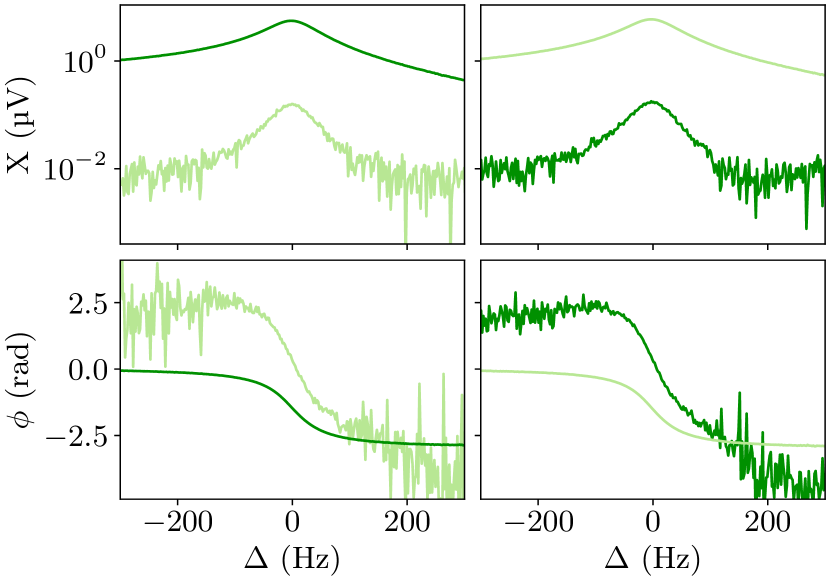
Figure 6: Linear response of coupled resonators. Phase and amplitude of both resonators while only one is driven by an external force. Left: resonator 1 is driven with $U_{f}=$20\text{\,}\mathrm{mV}$$ and resonator 2 follows. Right: resonator 2 is driven while 1 follows. The non-driven resonator generally shows a narrower peak in its amplitude response, resulting from the combination of its own response function with the frequency-dependent force amplitude it experiences from the externally driven resonator. Similarly, the phase of the non-driven resonator changes by $180\text{\,}\mathrm{\SIUnitSymbolDegree}$ when crossing the resonance, which is the sum of its own harmonic response phase and the phase of the driven partner.

References

- Ryvkine and Dykman (2006) D. Ryvkine and M. I. Dykman, “Resonant symmetry lifting in a parametrically modulated oscillator,” Phys. Rev. E 74, 061118 (2006).
- Mahboob and Yamaguchi (2008) I. Mahboob and H. Yamaguchi, “Bit storage and bit flip operations in an electromechanical oscillator,” Nature Nanotechnology 3, 275–279 (2008).
- Wilson et al. (2010) C. M. Wilson, T. Duty, M. Sandberg, F. Persson, V. Shumeiko, and P. Delsing, “Photon generation in an electromagnetic cavity with a time-dependent boundary,” Phys. Rev. Lett. 105, 233907 (2010).
- Eichler et al. (2011) Alexander Eichler, Julien Chaste, Joel Moser, and Adrian Bachtold, “Parametric amplification and self-oscillation in a nanotube mechanical resonator,” Nano Letters 11, 2699–2703 (2011).
- Leuch et al. (2016) Anina Leuch, Luca Papariello, Oded Zilberberg, Christian L. Degen, R. Chitra, and Alexander Eichler, “Parametric symmetry breaking in a nonlinear resonator,” Phys. Rev. Lett. 117, 214101 (2016).
- Gieseler et al. (2012) Jan Gieseler, Bradley Deutsch, Romain Quidant, and Lukas Novotny, “Subkelvin parametric feedback cooling of a laser-trapped nanoparticle,” Phys. Rev. Lett. 109, 103603 (2012).
- Lin et al. (2014) Z.R. Lin, K. Inomata, K. Koshino, W. D. Oliver, Y. Nakamura, J. S. Tsai, and T. Yamamoto, “Josephson parametric phase-locked oscillator and its application to dispersive readout of superconducting qubits,” Nature Communications 5, 4480 (2014).
- Puri et al. (2017a) S. Puri, S. Boutin, and A. Blais, “Engineering the quantum states of light in a kerr-nonlinear resonator by two-photon driving,” npj Quantum Information 3, 18 (2017a).
- Eichler et al. (2018) Alexander Eichler, Toni L. Heugel, Anina Leuch, Christian L. Degen, R. Chitra, and Oded Zilberberg, “A parametric symmetry breaking transducer,” Applied Physics Letters 112, 233105 (2018).
- Nosan et al. (2019) Z. Nosan, P. Märki, N. Hauff, C. Knaut, and A. Eichler, “Gate-controlled phase switching in a parametron,” Phys. Rev. E 99, 062205 (2019).
- Frimmer et al. (2019) Martin Frimmer, Toni L. Heugel, Ziga Nosan, Felix Tebbenjohanns, David Hälg, Abdulkadir Akin, Christian L. Degen, Lukas Novotny, R. Chitra, Oded Zilberberg, and Alexander Eichler, “Rapid flipping of parametric phase states,” Phys. Rev. Lett. 123, 254102 (2019).
- Grimm et al. (2020) Alexander Grimm, Nicholas E. Frattini, Shruti Puri, Shantanu O. Mundhada, Steven Touzard, Mazyar Mirrahimi, Steven M. Girvin, Shyam Shankar, and Michel H. Devoret, “Stabilization and operation of a kerr-cat qubit,” Nature 584, 205–209 (2020).
- Wang et al. (2019) Zhaoyou Wang, Marek Pechal, E. Alex Wollack, Patricio Arrangoiz-Arriola, Maodong Gao, Nathan R. Lee, and Amir H. Safavi-Naeini, “Quantum dynamics of a few-photon parametric oscillator,” Phys. Rev. X 9, 021049 (2019).
- Puri et al. (2019) Shruti Puri, Alexander Grimm, Philippe Campagne-Ibarcq, Alec Eickbusch, Kyungjoo Noh, Gabrielle Roberts, Liang Jiang, Mazyar Mirrahimi, Michel H. Devoret, and S. M. Girvin, “Stabilized cat in a driven nonlinear cavity: A fault-tolerant error syndrome detector,” Phys. Rev. X 9, 041009 (2019).
- Miller et al. (2019) James M.L. Miller, Dongsuk D. Shin, Hyun-Keun Kwon, Steven W. Shaw, and Thomas W. Kenny, “Phase control of self-excited parametric resonators,” Phys. Rev. Applied 12, 044053 (2019).
- Yamaji et al. (2022) T. Yamaji, S. Kagami, A. Yamaguchi, T. Satoh, K. Koshino, H. Goto, Z. R. Lin, Y. Nakamura, and T. Yamamoto, “Spectroscopic observation of the crossover from a classical duffing oscillator to a kerr parametric oscillator,” Phys. Rev. A 105, 023519 (2022).
- Ising (1925) Ernst Ising, “Beitrag zur theorie des ferromagnetismus,” Zeitschrift für Physik 31, 253–258 (1925).
- Mohseni et al. (2022) Naeimeh Mohseni, Peter L McMahon, and Tim Byrnes, “Ising machines as hardware solvers of combinatorial optimization problems,” Nature Reviews Physics , 1–17 (2022).
- Nigg et al. (2017) Simon E. Nigg, Niels Lörch, and Rakesh P. Tiwari, “Robust quantum optimizer with full connectivity,” Science Advances 3, e1602273 (2017).
- Inagaki et al. (2016a) Takahiro Inagaki, Yoshitaka Haribara, Koji Igarashi, Tomohiro Sonobe, Shuhei Tamate, Toshimori Honjo, Alireza Marandi, Peter L. McMahon, Takeshi Umeki, Koji Enbutsu, Osamu Tadanaga, Hirokazu Takenouchi, Kazuyuki Aihara, Ken-ichi Kawarabayashi, Kyo Inoue, Shoko Utsunomiya, and Hiroki Takesue, “A coherent ising machine for 2000-node optimization problems,” Science 354, 603–606 (2016a).
- Goto et al. (2019) Hayato Goto, Kosuke Tatsumura, and Alexander R Dixon, “Combinatorial optimization by simulating adiabatic bifurcations in nonlinear hamiltonian systems,” Science advances 5, eaav2372 (2019).
- Lucas (2014) Andrew Lucas, “Ising formulations of many np problems,” Frontiers in Physics 2, 5 (2014).
- Gottesman et al. (2001) Daniel Gottesman, Alexei Kitaev, and John Preskill, “Encoding a qubit in an oscillator,” Phys. Rev. A 64, 012310 (2001).
- Devoret and Schoelkopf (2013) M. H. Devoret and R. J. Schoelkopf, “Superconducting circuits for quantum information: An outlook,” Science 339, 1169–1174 (2013).
- Mahboob et al. (2016) Imran Mahboob, Hajime Okamoto, and Hiroshi Yamaguchi, “An electromechanical ising hamiltonian,” Science Advances 2, e1600236 (2016).
- Inagaki et al. (2016b) T. Inagaki, K Inaba, R. Hamerly, K Inoue, Y Yamamoto, and H. Takesue, “Large-scale ising spin network based on degenerate optical parametric oscillators,” Nature Photonics 10, 415–420 (2016b).
- Goto (2016) H. Goto, “Bifurcation-based adiabatic quantum computation with a nonlinear oscillator network,” Scientific Reports 6, 21686 (2016).
- Bello et al. (2019) Leon Bello, Marcello Calvanese Strinati, Emanuele G. Dalla Torre, and Avi Pe’er, “Persistent coherent beating in coupled parametric oscillators,” Phys. Rev. Lett. 123, 083901 (2019).
- Okawachi et al. (2020) Yoshitomo Okawachi, Mengjie Yu, Jae K. Jang, Xingchen Ji, Yun Zhao, Bok Young Kim, Michal Lipson, and Alexander L. Gaeta, “Demonstration of chip-based coupled degenerate optical parametric oscillators for realizing a nanophotonic spin-glass,” Nature Communications 11, 4119 (2020).
- Wang et al. (2013) Zhe Wang, Alireza Marandi, Kai Wen, Robert L. Byer, and Yoshihisa Yamamoto, “Coherent ising machine based on degenerate optical parametric oscillators,” Phys. Rev. A 88, 063853 (2013).
- Yamamoto et al. (2017) Yoshihisa Yamamoto, Kazuyuki Aihara, Timothee Leleu, Ken-ichi Kawarabayashi, Satoshi Kako, Martin Fejer, Kyo Inoue, and Hiroki Takesue, “Coherent ising machines—optical neural networks operating at the quantum limit,” npj Quantum Information 3, 49 (2017).
- Yamamura et al. (2017) Atsushi Yamamura, Kazuyuki Aihara, and Yoshihisa Yamamoto, “Quantum model for coherent ising machines: Discrete-time measurement feedback formulation,” Phys. Rev. A 96, 053834 (2017).
- Puri et al. (2017b) Shruti Puri, Christian Kraglund Andersen, Arne L. Grimsmo, and Alexandre Blais, “Quantum annealing with all-to-all connected nonlinear oscillators,” Nature Communications 8, 15785 (2017b).
- Goto et al. (2018) H. Goto, Z. Lin, and Y. Nakamura, “Boltzmann sampling from the ising model using quantum heating of coupled nonlinear oscillators,” Scientific Reports 8, 7154 (2018).
- Dykman et al. (2018) M. I. Dykman, Christoph Bruder, Niels Lörch, and Yaxing Zhang, “Interaction-induced time-symmetry breaking in driven quantum oscillators,” Phys. Rev. B 98, 195444 (2018).
- Rota et al. (2019) Riccardo Rota, Fabrizio Minganti, Cristiano Ciuti, and Vincenzo Savona, “Quantum critical regime in a quadratically driven nonlinear photonic lattice,” Phys. Rev. Lett. 122, 110405 (2019).
- Heugel et al. (2022a) Toni L. Heugel, Oded Zilberberg, Christian Marty, R. Chitra, and Alexander Eichler, “Ising machines with strong bilinear coupling,” Phys. Rev. Research 4, 013149 (2022a).
- Dykman et al. (1998) M. I. Dykman, C. M. Maloney, V. N. Smelyanskiy, and M. Silverstein, “Fluctuational phase-flip transitions in parametrically driven oscillators,” Phys. Rev. E 57, 5202–5212 (1998).
- Chan and Stambaugh (2007) H. B. Chan and C. Stambaugh, “Activation barrier scaling and crossover for noise-induced switching in micromechanical parametric oscillators,” Phys. Rev. Lett. 99, 060601 (2007).
- Chan et al. (2008) H. B. Chan, M. I. Dykman, and C. Stambaugh, “Paths of fluctuation induced switching,” Phys. Rev. Lett. 100, 130602 (2008).
- Mahboob et al. (2014) I. Mahboob, M. Mounaix, K. Nishiguchi, A. Fujiwara, and H. Yamaguchi, “A multimode electromechanical parametric resonator array,” Sci. Rep. 4, 4448 (2014).
- Margiani et al. (2022) Gabriel Margiani, Sebastián Guerrero, Toni L. Heugel, Christian Marty, Raphael Pachlatko, Thomas Gisler, Gabrielle D. Vukasin, Hyun-Keun Kwon, James M. L. Miller, Nicholas E. Bousse, Thomas W. Kenny, Oded Zilberberg, Deividas Sabonis, and Alexander Eichler, “Extracting the lifetime of a synthetic two-level system,” Applied Physics Letters 121, 164101 (2022).
- Yang et al. (2016) Yushi Yang, Eldwin J. Ng, Yunhan Chen, Ian B. Flader, and Thomas W. Kenny, “A Unified Epi-Seal Process for Fabrication of High-Stability Microelectromechanical Devices,” J. Microelectromechanical Syst. 25, 489–497 (2016).
- Agarwal et al. (2008) Manu Agarwal, Saurabh A. Chandorkar, Harsh Mehta, Robert N. Candler, Bongsang Kim, Matthew A. Hopcroft, Renata Melamud, Chandra M. Jha, Gaurav Bahl, Gary Yama, Thomas W. Kenny, and Boris Murmann, “A study of electrostatic force nonlinearities in resonant microstructures,” Appl. Phys. Lett. 92, 104106 (2008).
- Miller et al. (2022) James M.L. Miller, Anne L. Alter, Nicholas E. Bousse, Yunhan Chen, Ian B. Flader, Dongsuk D. Shin, Thomas W. Kenny, and Steven W. Shaw, “Influence of Clamping Loss and Electrical Damping On Nonlinear Dissipation in Micromechanical Resonators,” in 2022 IEEE 35th Int. Conf. Micro Electro Mech. Syst. Conf. (IEEE, 2022) pp. 507–510.
- Heugel et al. (2019) Toni L. Heugel, Matthias Oscity, Alexander Eichler, Oded Zilberberg, and R. Chitra, “Classical many-body time crystals,” Phys. Rev. Lett. 123, 124301 (2019).
- Heugel et al. (2022b) Toni L Heugel, Alexander Eichler, R Chitra, and Oded Zilberberg, “The role of fluctuations in quantum and classical time crystals,” arXiv preprint arXiv:2203.05577 (2022b).
- Dykman and Krivoglaz (1979) MI Dykman and MA Krivoglaz, “Theory of fluctuational transitions between stable states of a nonlinear oscillator,” Sov. Phys. JETP 50, 30–37 (1979).
- Dykman et al. (1993) M. I. Dykman, R. Mannella, P. V. E. McClintock, N. D. Stein, and N. G. Stocks, “Probability distributions and escape rates for systems driven by quasimonochromatic noise,” Phys. Rev. E 47, 3996–4009 (1993).
- Roychowdhury (2015) J. Roychowdhury, “Boolean computation using self-sustaining nonlinear oscillators,” Proceedings of the IEEE 103, 1958–1969 (2015).
- Strinati et al. (2020) Marcello Calvanese Strinati, Igal Aharonovich, Shai Ben-Ami, Emanuele G. Dalla Torre, Leon Bello, and Avi Pe’er, “Coherent dynamics in frustrated coupled parametric oscillators,” New J. Phys. 22, 085005 (2020), arXiv:2005.03562 .
- Lifshitz and Cross (2009) Ron Lifshitz and M. C. Cross, “Nonlinear Dynamics of Nanomechanical and Micromechanical Resonators,” in Rev. Nonlinear Dyn. Complex. (Wiley-VCH Verlag GmbH & Co. KGaA, Weinheim, Germany, 2009) pp. 1–52.
- Stambaugh and Chan (2006) C. Stambaugh and H. B. Chan, “Noise-activated switching in a driven nonlinear micromechanical oscillator,” Phys. Rev. B 73, 172302 (2006).
- Hänggi et al. (1990) Peter Hänggi, Peter Talkner, and Michal Borkovec, “Reaction-rate theory: fifty years after kramers,” Rev. Mod. Phys. 62, 251–341 (1990).
- Lehmann et al. (2003) J. Lehmann, P. Reimann, and P. Hänggi, “Activated escape over oscillating barriers: The case of many dimensions,” physica status solidi (b) 237, 53–71 (2003).
- Coffey (2013) William T. Coffey, “Path Integrals for Stochastic Processes: An Introduction, edited by Horacio S. Wio,” Contemp. Phys. 54, 268–268 (2013).