Is Out-of-Distribution Detection Learnable?

Abstract

Supervised learning aims to train a classifier under the assumption that training and test data are from the same distribution. To ease the above assumption, researchers have studied a more realistic setting: out-of-distribution (OOD) detection, where test data may come from classes that are unknown during training (i.e., OOD data). Due to the unavailability and diversity of OOD data, good generalization ability is crucial for effective OOD detection algorithms. To study the generalization of OOD detection, in this paper, we investigate the probably approximately correct (PAC) learning theory of OOD detection, which is proposed by researchers as an open problem. First, we find a necessary condition for the learnability of OOD detection. Then, using this condition, we prove several impossibility theorems for the learnability of OOD detection under some scenarios. Although the impossibility theorems are frustrating, we find that some conditions of these impossibility theorems may not hold in some practical scenarios. Based on this observation, we next give several necessary and sufficient conditions to characterize the learnability of OOD detection in some practical scenarios. Lastly, we also offer theoretical supports for several representative OOD detection works based on our OOD theory.

1 Introduction

The success of supervised learning is established on an implicit assumption that training and test data share a same distribution, i.e., in-distribution (ID) [1, 2, 3, 4]. However, test data distribution in many real-world scenarios may violate the assumption and, instead, contain out-of-distribution (OOD) data whose labels have not been seen during the training process [5, 6]. To mitigate the risk of OOD data, researchers have considered a more practical learning scenario: OOD detection which determines whether an input is ID/OOD, while classifying the ID data into respective classes. OOD detection has shown great potential to ensure the reliable deployment of machine learning models in the real world. A rich line of algorithms have been developed to empirically address the OOD detection problem [6, 7, 8, 9, 10, 11, 12, 13, 14, 15, 16, 17, 18, 19, 20]. However, very few works study theory of OOD detection, which hinders the rigorous path forward for the field. This paper aims to bridge the gap.

In this paper, we provide a theoretical framework to understand the learnability of the OOD detection problem. We investigate the probably approximately correct (PAC) learning theory of OOD detection, which is posed as an open problem to date. Unlike the classical PAC learning theory in a supervised setting, our problem setting is fundamentally challenging due to the absence of OOD data in training. In many real-world scenarios, OOD data can be diverse and priori-unknown. Given this, we study whether there exists an algorithm that can be used to detect various OOD data instead of merely some specified OOD data. Such is the significance of studying the learning theory for OOD detection [4]. This motivates our question: is OOD detection PAC learnable? i.e., is there the PAC learning theory to guarantee the generalization ability of OOD detection?

To investigate the learning theory, we mainly focus on two basic spaces: domain space and hypothesis space. The domain space is a space consisting of some distributions, and the hypothesis space is a space consisting of some classifiers. Existing agnostic PAC theories in supervised learning [21, 22] are distribution-free, i.e., the domain space consists of all domains. Yet, in Theorem 4, we shows that the learning theory of OOD detection is not distribution-free. In fact, we discover that OOD detection is learnable only if the domain space and the hypothesis space satisfy some special conditions, e.g., Conditions 1 and 3. Notably, there are many conditions and theorems in existing learning theories and many OOD detection algorithms in the literature. Thus, it is very difficult to analyze the relation between these theories and algorithms, and explore useful conditions to ensure the learnability of OOD detection, especially when we have to explore them from the scratch. Thus, the main aim of our paper is to study these essential conditions. From these essential conditions, we can know when OOD detection can be successful in practical scenarios. We restate our question and goal in following:

                  Given hypothesis spaces and several representative domain spaces, what are the conditions to ensure the learnability of OOD detection? If possible, we hope that these conditions are necessary and sufficient in some scenarios.

Main Results. We investigate the learnability of OOD detection starting from the largest space—the total space, and give a necessary condition (Condition 1) for the learnability. However, we find that the overlap between ID and OOD data may result in that the necessary condition does not hold. Therefore, we give an impossibility theorem to demonstrate that OOD detection fails in the total space (Theorem 4). Next, we study OOD detection in the separate space, where there are no overlaps between the ID and OOD data. Unfortunately, there still exists impossibility theorem (Theorem 5), which demonstrates that OOD detection is not learnable in the separate space under some conditions.

Although the impossibility theorems obtained in the separate space are frustrating, we find that some conditions of these impossibility theorems may not hold in some practical scenarios. Based on this observation, we give several necessary and sufficient conditions to characterize the learnability of OOD detection in the separate space (Theorems 6 and 10). Especially, when our model is based on fully-connected neural network (FCNN), OOD detection is learnable in the separate space if and only if the feature space is finite. Furthermore, we investigate the learnability of OOD detection in other more practical domain spaces, e.g., the finite-ID-distribution space (Theorem 8) and the density-based space (Theorem 9). By studying the finite-ID-distribution space, we discover a compatibility condition (Condition 3) that is a necessary and sufficient condition for this space. Next, we further investigate the compatibility condition in the density-based space, and find that such condition is also the necessary and sufficient condition in some practical scenarios (Theorem 11).

Implications and Impacts of Theory. Our study is not of purely theoretical interest; it has also practical impacts. First, when we design OOD detection algorithms, we normally only have finite ID datasets, corresponding to the finite-ID-distribution space. In this case, Theorem 8 gives the necessary and sufficient condition to the success of OOD detection. Second, our theory provides theoretical support (Theorems 10 and 11) for several representative OOD detection works [7, 8, 23]. Third, our theory shows that OOD detection is learnable in image-based scenarios when ID images have clearly different semantic labels and styles (far-OOD) from OOD images. Fourth, we should not expect a universally working algorithm. It is necessary to design different algorithms in different scenarios.

2 Learning Setups

We start by introducing the necessary concepts and notations for our theoretical framework. Given a feature space $\mathcal{X}\subset\mathbb{R}^{d}$ and a label space $\mathcal{Y}:=\{1,...,K\}$, we have an ID joint distribution $D_{X_{\rm I}Y_{\rm I}}$ over $\mathcal{X}\times\mathcal{Y}$, where $X_{\rm I}\in\mathcal{X}$ and $Y_{\rm I}\in\mathcal{Y}$ are random variables. We also have an OOD joint distribution $D_{X_{\rm O}Y_{\rm O}}$, where $X_{\rm O}$ is a random variable from $\mathcal{X}$, but $Y_{\rm O}$ is a random variable whose outputs do not belong to $\mathcal{Y}$. During testing, we will meet a mixture of ID and OOD joint distributions: $D_{XY}:=(1-\pi^{\rm out})D_{X_{\rm I}Y_{\rm I}}+\pi^{\rm out}D_{X_{\rm O}Y_{\rm O}}$, and can only observe the marginal distribution $D_{X}:=(1-\pi^{\rm out})D_{X_{\rm I}}+\pi^{\rm out}D_{X_{\rm O}}$, where the constant $\pi^{\rm out}\in[0,1)$ is an unknown class-prior probability.

Problem 1 (OOD Detection [4]).

Given an ID joint distribution $D_{X_{\rm I}Y_{\rm I}}$ and a training data $S:=\{(\mathbf{x}^{1},{y}^{1}),...,(\mathbf{x}^{n},{y}^{n})\}$ drawn independent and identically distributed from $D_{X_{\rm I}Y_{\rm I}}$, the aim of OOD detection is to train a classifier $f$ by using the training data $S$ such that, for any test data $\mathbf{x}$ drawn from the mixed marginal distribution $D_{X}$: 1) if $\mathbf{x}$ is an observation from $D_{X_{\rm I}}$, $f$ can classify $\mathbf{x}$ into correct ID classes; and 2) if $\mathbf{x}$ is an observation from $D_{X_{\rm O}}$, $f$ can detect $\mathbf{x}$ as OOD data.

According to the survey [4], when $K>1$, OOD detection is also known as the open-set recognition or open-set learning [24, 25]; and when $K=1$, OOD detection reduces to one-class novelty detection and semantic anomaly detection [26, 27, 28].

OOD Label and Domain Space. Based on Problem 1, we know it is not necessary to classify OOD data into the correct OOD classes. Without loss of generality, let all OOD data be allocated to one big OOD class, i.e., $Y_{\rm O}=K+1$ [24, 29]. To investigate the PAC learnability of OOD detection, we define a domain space $\mathscr{D}_{XY}$, which is a set consisting of some joint distributions $D_{XY}$ mixed by some ID joint distributions and some OOD joint distributions. In this paper, the joint distribution $D_{XY}$ mixed by ID joint distribution $D_{X_{\rm I}Y_{\rm I}}$ and OOD joint distribution $D_{X_{\rm O}Y_{\rm O}}$ is called domain.

Hypothesis Spaces and Scoring Function Spaces. A hypothesis space $\mathcal{H}$ is a subset of function space, i.e., $\mathcal{H}\subset\{{h}:\mathcal{X}\rightarrow\mathcal{Y}\cup\{K+1\}\}.$ We set $\mathcal{H}^{\rm in}\subset\{{h}:\mathcal{X}\rightarrow\mathcal{Y}\}$ to the ID hypothesis space. We also define $\mathcal{H}^{\rm b}\subset\{{h}:\mathcal{X}\rightarrow\{1,2\}\}$ as the hypothesis space for binary classification, where $1$ represents the ID data, and $2$ represents the OOD data. The function $h$ is called the hypothesis function. A scoring function space is a subset of function space, i.e., $\mathcal{F}_{l}\subset\{\mathbf{f}:\mathcal{X}\rightarrow\mathbb{R}^{l}\}$, where $l$ is the output’s dimension of the vector-valued function $\mathbf{f}$. The function $\mathbf{f}$ is called the scoring function.

Loss and Risks. Let $\mathcal{Y}_{\rm all}=\mathcal{Y}\cup\{K+1\}$. Given a loss function $\ell:\mathcal{Y}_{\rm all}\times\mathcal{Y}_{\rm all}\rightarrow\mathbb{R}_{\geq 0}$ satisfying that $\ell(y_{1},y_{2})=0$ if and only if $y_{1}=y_{2}$, and any ${h}\in\mathcal{H}$, then the risk with respect to ${D}_{XY}$ is

$$\begin{split}&R_{D}({h}):=\mathbb{E}_{(\mathbf{x},y)\sim D_{XY}}\ell({h}(\mathbf{x}),{y}).\end{split}$$ (1)

The $\alpha$-risk $R_{D}^{\alpha}({h}):=(1-\alpha)R^{\rm in}_{D}({h})+\alpha R^{\rm out}_{D}({h}),\forall\alpha\in[0,1]$, where the risks $R^{\rm in}_{D}({h})$, $R^{\rm out}_{D}({h})$ are

$$\begin{split}&R^{\rm in}_{D}({h}):=\mathbb{E}_{(\mathbf{x},y)\sim D_{X_{\rm I}Y_{\rm I}}}\ell({h}(\mathbf{x}),{y}),~{}~{}~{}~{}~{}~{}R^{\rm out}_{D}({h}):=\mathbb{E}_{\mathbf{x}\sim D_{X_{\rm O}}}\ell({h}(\mathbf{x}),K+1).\end{split}$$

Learnability. We aim to select a hypothesis function $h\in\mathcal{H}$ with approximately minimal risk, based on finite data. Generally, we expect the approximation to get better, with the increase in sample size. Algorithms achieving this are said to be consistent. Formally, we introduce the following definition:

Definition 1 (Learnability of OOD Detection).

Given a domain space $\mathscr{D}_{XY}$ and a hypothesis space $\mathcal{H}\subset\{{h}:\mathcal{X}\rightarrow\mathcal{Y}_{\rm all}\}$, we say OOD detection is learnable in $\mathscr{D}_{XY}$ for $\mathcal{H}$, if there exists an algorithm $\mathbf{A}:\cup_{n=1}^{+\infty}(\mathcal{X}\times\mathcal{Y})^{n}\rightarrow\mathcal{H}$ and a monotonically decreasing sequence $\epsilon_{\rm cons}(n)$, such that $\epsilon_{\rm cons}(n)\rightarrow 0$, as $n\rightarrow+\infty$, and for any domain $D_{XY}\in\mathscr{D}_{XY}$,

$$\mathbb{E}_{S\sim D^{n}_{X_{\rm I}Y_{\rm I}}}\big{[}R_{D}(\mathbf{A}(S))-\inf_{h\in\mathcal{H}}R_{D}(h)\big{]}\leq\epsilon_{\rm cons}(n),$$ (2)

An algorithm $\mathbf{A}$ for which this holds is said to be consistent with respect to $\mathscr{D}_{XY}$.

Definition 1 is a natural extension of agnostic PAC learnability of supervised learning [30]. If for any $D_{XY}\in\mathscr{D}_{XY}$, $\pi^{\rm out}=0$, then Definition 2 is the agnostic PAC learnability of supervised learning. Although the expression of Definition 1 is different from the normal definition of agnostic PAC learning in [21], one can easily prove that they are equivalent when $\ell$ is bounded, see Appendix D.3.

Since OOD data are unavailable, it is impossible to obtain information about the class-prior probability $\pi^{\rm out}$. Furthermore, in the real world, it is possible that $\pi^{\rm out}$ can be any value in $[0,1)$. Therefore, the imbalance issue between ID and OOD distributions, and the priori-unknown issue (i.e., $\pi^{\rm out}$ is unknown) are the core challenges. To ease these challenges, researchers use AUROC, AUPR and FPR95 to estimate the performance of OOD detection [18, 31, 32, 33, 34, 35]. It seems that there is a gap between Definition 1 and existing works. To eliminate this gap, we revise Eq. (2) as follows:

$$\begin{split}&\mathbb{E}_{S\sim D^{n}_{X_{\rm I}Y_{\rm I}}}\big{[}R_{D}^{\alpha}(\mathbf{A}(S))-\inf_{h\in\mathcal{H}}R_{D}^{\alpha}(h)\big{]}\leq\epsilon_{\rm cons}(n),~{}\forall\alpha\in[0,1].\end{split}$$ (3)

If an algorithm $\mathbf{A}$ satisfies Eq. (3), then the imbalance issue and the prior-unknown issue disappear. That is, $\mathbf{A}$ can simultaneously classify the ID data and detect the OOD data well. Based on the above discussion, we define the strong learnability of OOD detection as follows:

Definition 2 (Strong Learnability of OOD Detection).

Given a domain space $\mathscr{D}_{XY}$ and a hypothesis space $\mathcal{H}\subset\{{h}:\mathcal{X}\rightarrow\mathcal{Y}_{\rm all}\}$, we say OOD detection is strongly learnable in $\mathscr{D}_{XY}$ for $\mathcal{H}$, if there exists an algorithm $\mathbf{A}:\cup_{n=1}^{+\infty}(\mathcal{X}\times\mathcal{Y})^{n}\rightarrow\mathcal{H}$ and a monotonically decreasing sequence $\epsilon_{\rm cons}(n)$, such that $\epsilon_{\rm cons}(n)\rightarrow 0$, as $n\rightarrow+\infty$, and for any domain $D_{XY}\in\mathscr{D}_{XY}$,

$$\mathbb{E}_{S\sim D^{n}_{X_{\rm I}Y_{\rm I}}}\big{[}R_{D}^{\alpha}(\mathbf{A}(S))-\inf_{h\in\mathcal{H}}R_{D}^{\alpha}(h)\big{]}\leq\epsilon_{\rm cons}(n),~{}\forall\alpha\in[0,1].$$

In Theorem 1, we have shown that the strong learnability of OOD detection is equivalent to the learnability of OOD detection, if the domain space $\mathscr{D}_{XY}$ is a prior-unknown space (see Definition 3). In this paper, we mainly discuss the learnability in the prior-unknown space. Therefore, when we mention that OOD detection is learnable, we also mean that OOD detection is strongly learnable.

Goal of Theory. Note that the agnostic PAC learnability of supervised learning is distribution-free, i.e., the domain space $\mathscr{D}_{XY}$ consists of all domains. However, due to the absence of OOD data during the training process [8, 14, 24], it is obvious that the learnability of OOD detection is not distribution-free (i.e., Theorem 4). In fact, we discover that the learnability of OOD detection is deeply correlated with the relationship between the domain space $\mathscr{D}_{XY}$ and the hypothesis space $\mathcal{H}$. That is, OOD detection is learnable only when the domain space $\mathscr{D}_{XY}$ and the hypothesis space $\mathcal{H}$ satisfy some special conditions, e.g., Condition 1 and Condition 3. We present our goal as follows:

           Goal: given a hypothesis space $\mathcal{H}$ and several representative domain spaces $\mathscr{D}_{XY}$, what are the conditions to ensure the learnability of OOD detection? Furthermore, if possible, we hope that these conditions are necessary and sufficient in some scenarios.

Therefore, compared to the agnostic PAC learnability of supervised learning, our theory doesn’t focus on the distribution-free case, but focuses on discovering essential conditions to guarantee the learnability of OOD detection in several representative and practical domain spaces $\mathscr{D}_{XY}$. By these essential conditions, we can know when OOD detection can be successful in real applications.

3 Learning in Priori-unknown Spaces

We first investigate a special space, called prior-unknown space. In such space, Definition 1 and Definition 2 are equivalent. Furthermore, we also prove that if OOD detection is strongly learnable in a space $\mathscr{D}_{XY}$, then one can discover a larger domain space, which is prior-unknown, to ensure the learnability of OOD detection. These results imply that it is enough to consider our theory in the prior-unknown spaces. The prior-unknown space is introduced as follows:

Definition 3.

Given a domain space $\mathscr{D}_{XY}$, we say $\mathscr{D}_{XY}$ is a priori-unknown space, if for any domain $D_{XY}\in\mathscr{D}_{XY}$ and any $\alpha\in[0,1)$, we have $D_{XY}^{\alpha}:=(1-\alpha)D_{X_{\rm I}Y_{\rm I}}+\alpha D_{X_{\rm O}Y_{\rm O}}\in\mathscr{D}_{XY}$.

Theorem 1.

Given domain spaces $\mathscr{D}_{XY}$ and $\mathscr{D}_{XY}^{\prime}=\{D_{XY}^{\alpha}:\forall D_{XY}\in\mathscr{D}_{XY},\forall\alpha\in[0,1)\}$, then
1) $\mathscr{D}_{XY}^{\prime}$ is a priori-unknown space and $\mathscr{D}_{XY}\subset\mathscr{D}_{XY}^{\prime}$;
2) if $\mathscr{D}_{XY}$ is a priori-unknown space, then Definition 1 and Definition 2 are equivalent;
3) OOD detection is strongly learnable in $\mathscr{D}_{XY}$ if and only if OOD detection is learnable in $\mathscr{D}_{XY}^{\prime}$.

The second result of Theorem 1 bridges the learnability and strong learnability, which implies that if an algorithm $\mathbf{A}$ is consistent with respect to a prior-unknown space, then this algorithm $\mathbf{A}$ can address the imbalance issue between ID and OOD distributions, and the priori-unknown issue well. Based on Theorem 1, we focus on our theory in the prior-unknown spaces. Furthermore, to demystify the learnability of OOD detection, we introduce five representative priori-unknown spaces:

$\bullet$ Single-distribution space $\mathscr{D}_{XY}^{D_{XY}}$. For a domain $D_{XY}$, $\mathscr{D}_{XY}^{D_{XY}}:=\{D_{XY}^{\alpha}:\forall\alpha\in[0,1)\}$.
$\bullet$ Total space $\mathscr{D}_{XY}^{\rm all}$, which consists of all domains.
$\bullet$ Separate space $\mathscr{D}_{XY}^{s}$, which consists of all domains that satisfy the separate condition, that is for any $D_{XY}\in\mathscr{D}_{XY}^{s}$, ${\rm supp}D_{X_{\rm O}}\cap{\rm supp}D_{X_{\rm I}}=\emptyset,$ where ${\rm supp}$ means the support set.
$\bullet$ Finite-ID-distribution space $\mathscr{D}_{XY}^{F}$, which is a prior-unknown space satisfying that the number of distinct ID joint distributions $D_{X_{\rm I}Y_{\rm I}}$ in $\mathscr{D}_{XY}^{F}$ is finite, i.e., $|\{D_{X_{\rm I}Y_{\rm I}}:\forall D_{XY}\in\mathscr{D}_{XY}^{F}\}|<+\infty$.
$\bullet$ Density-based space $\mathscr{D}^{\mu,b}_{XY}$, which is a prior-unknown space consisting of some domains satisfying that: for any $D_{XY}$, there exists a density function $f$ with $1/b\leq f\leq b$ in ${\rm supp}\mu$ and $0.5*D_{X_{\rm I}}+0.5*D_{X_{\rm O}}=\int f{\rm d}\mu$, where $\mu$ is a measure defined over $\mathcal{X}$. Note that if $\mu$ is discrete, then $D_{X}$ is a discrete distribution; and if $\mu$ is the Lebesgue measure, then $D_{X}$ is a continuous distribution.

The above representative spaces widely exist in real applications. For example, 1) if the images from different semantic labels with different styles are clearly different, then those images can form a distribution belonging to a separate space $\mathscr{D}_{XY}^{s}$; and 2) when designing an algorithm, we only have finite ID datasets, e.g., CIFAR-10, MNIST, SVHN, and ImageNet, to build a model. Then, finite-ID-distribution space $\mathscr{D}_{XY}^{F}$ can handle this real scenario. Note that the single-distribution space is a special case of the finite-ID-distribution space. In this paper, we mainly discuss these five spaces.

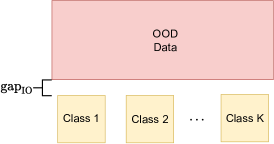
(a) ID and OOD Distributions

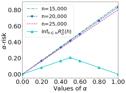
(b) Overlap Exists

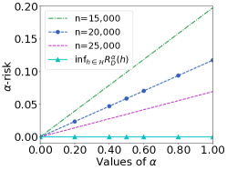
(c) No Overlap

Figure 1: Illustration of $\inf_{h\in\mathcal{H}}R_{D}^{\alpha}({h})$ (solid lines with triangle marks) and the estimated $\mathbb{E}_{S\sim D^{n}_{\rm in}}R^{\alpha}_{D}(\mathbf{A}(S))$ (dash lines) with $\alpha\in[0,1)$ in different scenarios, where $D_{\rm in}=D_{X_{\rm I}Y_{\rm I}}$ and the algorithm $\mathbf{A}$ is the free-energy OOD detection method [23]. Subfigure (a) shows the ID and OOD distributions. In (a), ${\rm gap}_{\rm IO}$ represents the distance between the support sets of ID and OOD distributions. In (b), since there is an overlap between ID and OOD data, the solid line is a ployline. In (c), since there is no overlap between ID and OOD data, we can check that $\inf_{h\in\mathcal{H}}R_{D}^{\alpha}({h})$ forms a straight line (the solid line). However, since dash lines are always straight lines, two observations can be obtained from (b) and (c): 1) dash lines cannot approximate the solid ployline in (b), which implies the unlearnability of OOD detection; and 2) the solid line in (c) is a straight line and may be approximated by the dash lines in (c). The above observations motivate us to propose Condition 1.

4 Impossibility Theorems for OOD Detection

In this section, we first give a necessary condition for the learnability of OOD detection. Then, we show this necessary condition does not hold in the total space $\mathscr{D}_{XY}^{\rm all}$ and the separate space $\mathscr{D}_{XY}^{s}$.

Necessary Condition. We find a necessary condition for the learnability of OOD detection, i.e., Condition 1, motivated by the experiments in Figure 1. Details of Figure 1 can be found in Appendix C.2.

Condition 1 (Linear Condition).

For any $D_{XY}\in\mathscr{D}_{XY}$ and any $\alpha\in[0,1)$,

$$\inf_{h\in\mathcal{H}}R_{D}^{\alpha}(h)=(1-\alpha)\inf_{h\in\mathcal{H}}R_{D}^{\rm in}(h)+\alpha\inf_{h\in\mathcal{H}}R_{D}^{\rm out}(h).$$

To reveal the importance of Condition 1, Theorem 2 shows that Condition 1 is a necessary and sufficient condition for the learnability of OOD detection if the $\mathscr{D}_{XY}$ is the single-distribution space.

Theorem 2.

Given a hypothesis space $\mathcal{H}$ and a domain $D_{XY}$, OOD detection is learnable in the single-distribution space $\mathscr{D}_{XY}^{D_{XY}}$ for $\mathcal{H}$ if and only if linear condition (i.e., Condition 1) holds.

Theorem 2 implies that Condition 1 is important for the learnability of OOD detection. Due to the simplicity of single-distribution space, Theorem 2 implies that Condition 1 is the necessary condition for the learnability of OOD detection in the prior-unknown space, see Lemma 1 in Appendix F.

Impossibility Theorems. Here, we first study whether Condition 1 holds in the total space $\mathscr{D}_{XY}^{\rm all}$. If Condition 1 does not hold, then OOD detection is not learnable. Theorem 3 shows that Condition 1 is not always satisfied, especially, when there is an overlap between the ID and OOD distributions:

Definition 4 (Overlap Between ID and OOD).

We say a domain $D_{XY}$ has overlap between ID and OOD distributions, if there is a $\sigma$-finite measure $\tilde{\mu}$ such that $D_{X}$ is absolutely continuous with respect to $\tilde{\mu}$, and $\tilde{\mu}(A_{\rm overlap})>0,~{}\textit{ where}$ $A_{\rm overlap}=\{\mathbf{x}\in\mathcal{X}:f_{\rm I}(\mathbf{x})>0~{}\textit{and}~{}f_{\rm O}(\mathbf{x})>0\}$. Here $f_{\rm I}$ and $f_{\rm O}$ are the representers of $D_{X_{\rm I}}$ and $D_{X_{\rm O}}$ in Radon–Nikodym Theorem [36],

$$D_{X_{\rm I}}=\int f_{\rm I}{\rm d}\tilde{\mu},~{}~{}~{}D_{X_{\rm O}}=\int f_{\rm O}{\rm d}\tilde{\mu}.$$

Theorem 3.

Given a hypothesis space $\mathcal{H}$ and a prior-unknown space $\mathscr{D}_{XY}$, if there is $D_{XY}\in\mathscr{D}_{XY}$, which has overlap between ID and OOD, and $\inf_{h\in\mathcal{H}}R_{D}^{\rm in}(h)=0$ and $\inf_{h\in\mathcal{H}}R_{D}^{\rm out}(h)=0$, then Condition 1 does not hold. Therefore, OOD detection is not learnable in $\mathscr{D}_{XY}$ for $\mathcal{H}$.

Theorem 3 clearly shows that under proper conditions, Condition 1 does not hold, if there exists a domain whose ID and OOD distributions have overlap. By Theorem 3, we can obtain that the OOD detection is not learnable in the total space $\mathscr{D}^{\rm all}_{XY}$ for any non-trivial hypothesis space $\mathcal{H}$.

Theorem 4 (Impossibility Theorem for Total Space).

OOD detection is not learnable in the total space $\mathscr{D}^{\rm all}_{XY}$ for $\mathcal{H}$, if $|\phi\circ\mathcal{H}|>1$, where $\phi$ maps ID labels to $1$ and maps OOD labels to $2$.

Since the overlaps between ID and OOD distributions may cause that Condition 1 does not hold, we then consider studying the learnability of OOD detection in the separate space $\mathscr{D}_{XY}^{s}$, where there are no overlaps between the ID and OOD distributions. However, Theorem 5 shows that even if we consider the separate space, the OOD detection is still not learnable in some scenarios. Before introducing the impossibility theorem for separate space, i.e., Theorem 5, we need a mild assumption:

Assumption 1 (Separate Space for OOD).

A hypothesis space $\mathcal{H}$ is separate for OOD data, if for each data point $\mathbf{x}\in\mathcal{X}$, there exists at least one hypothesis function $h_{\mathbf{x}}\in\mathcal{H}$ such that $h_{\mathbf{x}}(\mathbf{x})=K+1$.

Assumption 1 means that every data point $\mathbf{x}$ has the possibility to be detected as OOD data. Assumption 1 is mild and can be satisfied by many hypothesis spaces, e.g., the FCNN-based hypothesis space (Proposition 1 in Appendix K), score-based hypothesis space (Proposition 2 in Appendix K) and universal kernel space. Next, we use Vapnik–Chervonenkis (VC) dimension [22] to measure the size of hypothesis space, and study the learnability of OOD detection in $\mathscr{D}_{XY}^{s}$ based on the VC dimension.

Theorem 5 (Impossibility Theorem for Separate Space).

If Assumption 1 holds, ${\rm VCdim}(\phi\circ\mathcal{H})<+\infty$ and $\sup_{{h}\in\mathcal{H}}|\{\mathbf{x}\in\mathcal{X}:{h}(\mathbf{x})\in\mathcal{Y}\}|=+\infty$, then OOD detection is not learnable in separate space $\mathscr{D}_{XY}^{s}$ for $\mathcal{H}$, where $\phi$ maps ID labels to ${1}$ and maps OOD labels to $2$.

The finite VC dimension normally implies the learnability of supervised learning. However, in our results, the finite VC dimension cannot guarantee the learnability of OOD detection in the separate space, which reveals the difficulty of the OOD detection. Although the above impossibility theorems are frustrating, there is still room to discuss the conditions in Theorem 5, and to find out the proper conditions for ensuring the learnability of OOD detection in the separate space (see Sections 5 and 6).

5 When OOD Detection Can Be Successful

Here, we discuss when the OOD detection can be learnable in the separate space $\mathscr{D}_{XY}^{s}$, finite-ID-distribution space $\mathscr{D}_{XY}^{F}$ and density-based space $\mathscr{D}_{XY}^{\mu,b}$. We first study the separate space $\mathscr{D}_{XY}^{s}$.

OOD Detection in the Separate Space. Theorem 5 has indicated that ${\rm VCdim}(\phi\circ\mathcal{H})=+\infty$ or $\sup_{{h}\in\mathcal{H}}|\{\mathbf{x}\in\mathcal{X}:{h}(\mathbf{x})\in\mathcal{Y}\}|<+\infty$ is necessary to ensure the learnability of OOD detection in $\mathscr{D}_{XY}^{s}$ if Assumption 1 holds. However, generally, hypothesis spaces generated by feed-forward neural networks with proper activation functions have finite VC dimension [37, 38]. Therefore, we study the learnability of OOD detection in the case that $|\mathcal{X}|<+\infty$, which implies that $\sup_{{h}\in\mathcal{H}}|\{\mathbf{x}\in\mathcal{X}:{h}(\mathbf{x})\in\mathcal{Y}\}|<+\infty$. Additionally, Theorem 10 also implies that $|\mathcal{X}|<+\infty$ is the necessary and sufficient condition for the learnability of OOD detection in separate space, when the hypothesis space is generated by FCNN. Hence, $|\mathcal{X}|<+\infty$ may be necessary in the space $\mathscr{D}_{XY}^{s}$.

For simplicity, we first discuss the case that $K=1$, i.e., the one-class novelty detection. We show the necessary and sufficient condition for the learnability of OOD detection in $\mathscr{D}_{XY}^{s}$, when $|\mathcal{X}|<+\infty$.

Theorem 6.

Let $K=1$ and $|\mathcal{X}|<+\infty$. Suppose that Assumption 1 holds and the constant function $h^{\rm in}:=1\in\mathcal{H}$. Then OOD detection is learnable in $\mathscr{D}_{XY}^{s}$ for $\mathcal{H}$ if and only if $\mathcal{H}_{\rm all}-\{h^{\rm out}\}\subset\mathcal{H}$, where $\mathcal{H}_{\rm all}$ is the hypothesis space consisting of all hypothesis functions, and $h^{\rm out}$ is a constant function that $h^{\rm out}:=2$, here $1$ represents ID data and $2$ represents OOD data.

The condition $h^{\rm in}\in\mathcal{H}$ presented in Theorem 6 is mild. Many practical hypothesis spaces satisfy this condition, e.g., the FCNN-based hypothesis space (Proposition 1 in Appendix K), score-based hypothesis space (Proposition 2 in Appendix K) and universal kernel-based hypothesis space. Theorem 6 implies that if $K=1$ and OOD detection is learnable in $\mathscr{D}^{s}_{XY}$ for $\mathcal{H}$, then the hypothesis space $\mathcal{H}$ should contain almost all hypothesis functions, implying that if the OOD detection can be learnable in the distribution-agnostic case, then a large-capacity model is necessary.

Next, we extend Theorem 6 to a general case, i.e., $K>1$. When $K>1$, we will first use a binary classifier $h^{b}$ to classify the ID and OOD data. Then, for the ID data identified by $h^{b}$, an ID hypothesis function $h^{\rm in}$ will be used to classify them into corresponding ID classes. We state this strategy as follows: given a hypothesis space $\mathcal{H}^{\rm in}$ for ID distribution and a binary classification hypothesis space $\mathcal{H}^{\rm b}$ introduced in Section 2, we use $\mathcal{H}^{\rm in}$ and $\mathcal{H}^{\rm b}$ to construct an OOD detection’s hypothesis space $\mathcal{H}$, which consists of all hypothesis functions $h$ satisfying the following condition: there exist $h^{\rm in}\in\mathcal{H}^{\rm in}$ and $h^{\rm b}\in\mathcal{H}^{b}$ such that for any $\mathbf{x}\in\mathcal{X}$,

$$h(\mathbf{x})=i,~{}~{}\textnormal{ if}~{}h^{\rm in}(\mathbf{x})=i~{}\textnormal{ and }~{}h^{\rm b}(\mathbf{x})=1;\textnormal{ otherwise},~{}h(\mathbf{x})=K+1.$$ (4)

We use $\mathcal{H}^{\rm in}\bullet\mathcal{H}^{\rm b}$ to represent a hypothesis space consisting of all $h$ defined in Eq. (4). In addition, we also need an additional condition for the loss function $\ell$. This condition is shown as follows:

Condition 2.

$\ell(y_{2},y_{1})\leq\ell(K+1,y_{1})$, for any in-distribution labels $y_{1}$ and $y_{2}\in\mathcal{Y}.$

Theorem 7.

Let $|\mathcal{X}|<+\infty$ and $\mathcal{H}=\mathcal{H}^{\rm in}\bullet\mathcal{H}^{\rm b}$. If $\mathcal{H}_{\rm all}-\{h^{\rm out}\}\subset\mathcal{H}^{\rm b}$ and Condition 2 holds, then OOD detection is learnable in $\mathscr{D}_{XY}^{s}$ for $\mathcal{H}$, where $\mathcal{H}_{\rm all}$ and $h^{\rm out}$ are defined in Theorem 6.

OOD Detection in the Finite-ID-Distribution Space. Since researchers can only collect finite ID datasets as the training data in the process of algorithm design, it is worthy to study the learnability of OOD detection in the finite-ID-distribution space $\mathscr{D}_{XY}^{F}$. We first show two necessary concepts below.

Definition 5 (ID Consistency).

Given a domain space $\mathscr{D}_{XY}$, we say any two domains $D_{XY}\in\mathscr{D}_{XY}$ and $D_{XY}^{\prime}\in\mathscr{D}_{XY}$ are ID consistency, if $D_{X_{\rm I}Y_{\rm I}}=D_{X_{\rm I}Y_{\rm I}}^{\prime}$. We use the notation $\sim$ to represent the ID consistency, i.e., $D_{XY}\sim D_{XY}^{\prime}$ if and only if $D_{XY}$ and $D_{XY}^{\prime}$ are ID consistency.

It is easy to check that the ID consistency $\sim$ is an equivalence relation. Therefore, we define the set $[D_{XY}]:=\{D_{XY}^{\prime}\in\mathscr{D}_{XY}:D_{XY}\sim D_{XY}^{\prime}\}$ as the equivalence class with respect to space $\mathscr{D}_{XY}$.

Condition 3 (Compatibility).

For any equivalence class $[D_{XY}^{\prime}]$ with respect to $\mathscr{D}_{XY}$ and any $\epsilon>0$, there exists a hypothesis function $h_{\epsilon}\in\mathcal{H}$ such that for any domain $D_{XY}\in[D_{XY}^{\prime}]$,

$$h_{\epsilon}\in\{h^{\prime}\in\mathcal{H}:R_{D}^{\rm out}(h^{\prime})\leq\inf_{h\in\mathcal{H}}R_{D}^{\rm out}(h)+\epsilon\}\cap\{h^{\prime}\in\mathcal{H}:R_{D}^{\rm in}(h^{\prime})\leq\inf_{h\in\mathcal{H}}R_{D}^{\rm in}(h)+\epsilon\}.$$

In Appendix F, Lemma 2 has implied that Condition 3 is a general version of Condition 1. Next, Theorem 8 indicates that Condition 3 is the necessary and sufficient condition in the space $\mathscr{D}_{XY}^{F}$.

Theorem 8.

Suppose that $\mathcal{X}$ is a bounded set. OOD detection is learnable in the finite-ID-distribution space $\mathscr{D}_{XY}^{F}$ for $\mathcal{H}$ if and only if the compatibility condition (i.e., Condition 3) holds. Furthermore, the learning rate $\epsilon_{\rm cons}(n)$ can attain ${O}(1/\sqrt{n^{1-\theta}})$, for any $\theta\in(0,1)$.

Theorem 8 shows that, in the process of algorithm design, OOD detection cannot be successful without the compatibility condition. Theorem 8 also implies that Condition 3 is essential for the learnability of OOD detection. This motivates us to study whether OOD detection can be successful in more general spaces (e.g., the density-based space), when the compatibility condition holds.

OOD Detection in the Density-based Space. To ensure that Condition 3 holds, we consider a basic assumption in learning theory—Realizability Assumption (see Appendix D.2), i.e., for any $D_{XY}\in\mathscr{D}_{XY}$, there exists $h^{*}\in\mathcal{H}$ such that $R_{D}(h^{*})=0$. We discover that in the density-based space $\mathscr{D}_{XY}^{\mu,b}$, Realizability Assumption can conclude the compatibility condition (i.e., Condition 3). Based on this observation, we can prove the following theorem:

Theorem 9.

Given a density-based space $\mathscr{D}_{XY}^{\mu,b}$, if $\mu(\mathcal{X})<+\infty$, the Realizability Assumption holds, then when $\mathcal{H}$ has finite Natarajan dimension [21], OOD detection is learnable in $\mathscr{D}_{XY}^{\mu,b}$ for $\mathcal{H}$. Furthermore, the learning rate $\epsilon_{\rm cons}(n)$ can attain ${O}(1/\sqrt{n^{1-\theta}})$, for any $\theta\in(0,1)$.

To further investigate the importance and necessary of Realizability Assumption, Theorem 11 has indicated that in some practical scenarios, Realizability Assumption is the necessary and sufficient condition for the learnability of OOD detection in the density-based space. Therefore, Realizability Assumption may be indispensable for the learnability of OOD detection in some practical scenarios.

6 Connecting Theory to Practice

In Section 5, we have shown the successful scenarios where OOD detection problem can be addressed in theory. In this section, we will discuss how the proposed theory is applied to two representative hypothesis spaces—neural-network-based hypothesis spaces and score-based hypothesis spaces.

Fully-connected Neural Networks. Given a sequence $\mathbf{q}=(l_{1},l_{2},...,l_{g})$, where $l_{i}$ and $g$ are positive integers and $g>2$, we use $g$ to represent the depth of neural network and use $l_{i}$ to represent the width of the $i$-th layer. After the activation function $\sigma$ is selected, we can obtain the architecture of FCNN according to the sequence $\mathbf{q}$. Let $\mathbf{f}_{\mathbf{w},\mathbf{b}}$ be the function generated by FCNN with weights $\mathbf{w}$ and bias $\mathbf{b}$. An FCNN-based scoring function space is defined as: $\mathcal{F}_{\mathbf{q}}^{\sigma}:=\{\mathbf{f}_{\mathbf{w},\mathbf{b}}:\forall~{}\textnormal{weights}~{}\mathbf{w},~{}\forall~{}\textnormal{bias}~{}\mathbf{b}\}.$ In addition, for simplicity, given any two sequences $\mathbf{q}=(l_{1},...,l_{g})$ and $\mathbf{q}^{\prime}=(l_{1}^{\prime},...,l_{g^{\prime}}^{\prime})$, we use the notation $\mathbf{q}\lesssim\mathbf{q}^{\prime}$ to represent the following equations and inequalities:

$$1)~{}g\leq g^{\prime},l_{1}=l_{1}^{\prime},l_{g}=l_{g^{\prime}}^{\prime};~{}~{}~{}~{}~{}2)~{}l_{i}\leq l^{\prime}_{i},~{}\forall i=1,...,g-1;~{}~{}\textnormal{and}~{}~{}~{}3)~{}l_{g-1}\leq l^{\prime}_{i},~{}\forall i=g,...,g^{\prime}-1.$$

In Appendix L, Lemma 10 shows $\mathbf{q}\lesssim\mathbf{q}^{\prime}\Rightarrow\mathcal{F}_{\mathbf{q}}^{\sigma}\subset\mathcal{F}_{\mathbf{q}^{\prime}}^{\sigma}$. We use $\lesssim$ to compare the sizes of FCNNs.

FCNN-based Hypothesis Space. Let $l_{g}=K+1$. The FCNN-based scoring function space $\mathcal{F}_{\mathbf{q}}^{\sigma}$ can induce an FCNN-based hypothesis space. For any $\mathbf{f}_{\mathbf{w},\mathbf{b}}\in\mathcal{F}_{\mathbf{q}}^{\sigma}$, the induced hypothesis function is:

$$h_{\mathbf{w},\mathbf{b}}:=\operatorname*{arg\,max}_{k\in\{1,...,K+1\}}{f}^{k}_{\mathbf{w},\mathbf{b}},~{}\textnormal{where}~{}{f}^{k}_{\mathbf{w},\mathbf{b}}~{}\textnormal{is ~{}the~{}}k\textnormal{-th}~{}\textnormal{coordinate~{}of}~{}\mathbf{f}_{\mathbf{w},\mathbf{b}}.$$

Then, the FCNN-based hypothesis space is defined as $\mathcal{H}_{\mathbf{q}}^{\sigma}:=\{h_{\mathbf{w},\mathbf{b}}:\forall~{}\textnormal{weights}~{}\mathbf{w},~{}\forall~{}\textnormal{bias}~{}\mathbf{b}\}.$

Score-based Hypothesis Space. Many OOD detection algorithms detect OOD data by using a score-based strategy. That is, given a threshold $\lambda$, a scoring function space $\mathcal{F}_{l}\subset\{\mathbf{f}:\mathcal{X}\rightarrow\mathbb{R}^{l}\}$ and a scoring function $E:\mathcal{F}_{l}\rightarrow\mathbb{R}$, then $\mathbf{x}$ is regarded as ID data if and only if $E(\mathbf{f}(\mathbf{x}))\geq\lambda$. We introduce several representative scoring functions $E$ as follows: for any $\mathbf{f}=[f^{1},...,f^{l}]^{\top}\in\mathcal{F}_{l}$,
$\bullet$ softmax-based function [7] and temperature-scaled function [8]: $\lambda\in(\frac{1}{l},1)$ and $T>0$,

$$E(\mathbf{f})=\max_{k\in\{1,...,l\}}\frac{\exp{(f^{k})}}{\sum_{c=1}^{l}\exp{(f^{c})}},~{}~{}~{}~{}~{}~{}~{}E(\mathbf{f})=\max_{k\in\{1,...,l\}}\frac{\exp{(f^{k}/T)}}{\sum_{c=1}^{l}\exp{(f^{c}/T)}};$$ (5)

$\bullet$ energy-based function [23]: $\lambda\in(0,+\infty)$ and $T>0$,

$$E(\mathbf{f})=T\log\sum_{c=1}^{l}\exp{(f^{c}/T)}.~{}~{}~{}$$ (6)

Using $E$, $\lambda$ and $\mathbf{f}\in\mathcal{F}_{\mathbf{q}}^{\sigma}$, we have a classifier: $h^{\lambda}_{\mathbf{f},E}(\mathbf{x})=1$, if $E(\mathbf{f}(\mathbf{x}))\geq\lambda$; otherwise, $h^{\lambda}_{\mathbf{f},E}(\mathbf{x})=2$, where $1$ represents the ID data and $2$ represents the OOD data. Hence, a binary classification hypothesis space $\mathcal{H}^{b}$, which consists of all $h^{\lambda}_{\mathbf{f},E}$, is generated. We define $\mathcal{H}^{{\sigma},\lambda}_{{\mathbf{q}},E}:=\{h^{\lambda}_{\mathbf{f},E}:\forall\mathbf{f}\in\mathcal{F}_{\mathbf{q}}^{\sigma}\}$.

Learnability of OOD Detection in Different Hypothesis Spaces. Next, we present applications of our theory regarding the above two practical and important hypothesis spaces $\mathcal{H}_{\mathbf{q}}^{\sigma}$ and $\mathcal{H}_{\mathbf{q},E}^{\sigma,\lambda}$.

Theorem 10.

Suppose that Condition 2 holds and the hypothesis space $\mathcal{H}$ is FCNN-based or score-based, i.e., $\mathcal{H}=\mathcal{H}_{\mathbf{q}}^{\sigma}$ or $\mathcal{H}=\mathcal{H}^{\rm in}\bullet\mathcal{H}^{\rm b}$, where $\mathcal{H}^{\rm in}$ is an ID hypothesis space, $\mathcal{H}^{\rm b}=\mathcal{H}^{{\sigma},\lambda}_{{\mathbf{q}},E}$ and $\mathcal{H}=\mathcal{H}^{\rm in}\bullet\mathcal{H}^{\rm b}$ is introduced below Eq. (4), here $E$ is introduced in Eqs. (5) or (6). Then
                         There is a sequence $\mathbf{q}=(l_{1},...,l_{g})$ such that OOD detection is learnable in the separate space $\mathscr{D}^{s}_{XY}$ for $\mathcal{H}$ if and only if $|\mathcal{X}|<+\infty$.
Furthermore, if $|\mathcal{X}|<+\infty$, then there exists a sequence $\mathbf{q}=(l_{1},...,l_{g})$ such that for any sequence $\mathbf{q}^{\prime}$ satisfying that $\mathbf{q}\lesssim\mathbf{q}^{\prime}$, OOD detection is learnable in $\mathscr{D}^{s}_{XY}$ for $\mathcal{H}$.

Theorem 10 states that 1) when the hypothesis space is FCNN-based or score-based, the finite feature space is the necessary and sufficient condition for the learnability of OOD detection in the separate space; and 2) a larger architecture of FCNN has a greater probability to achieve the learnability of OOD detection in the separate space. Note that when we select Eqs. (5) or (6) as the scoring function $E$, Theorem 10 also shows that the selected scoring functions $E$ can guarantee the learnability of OOD detection, which is a theoretical support for the representative works [8, 23, 7]. Furthermore, Theorem 11 also offers theoretical supports for these works in the density-based space, when $K=1$.

Theorem 11.

Suppose that each domain $D_{XY}$ in $\mathscr{D}_{XY}^{\mu,b}$ is attainable, i.e., $\operatorname*{arg\,min}_{h\in\mathcal{H}}R_{D}(h)\neq\emptyset$ (the finite discrete domains satisfy this). Let $K=1$ and the hypothesis space $\mathcal{H}$ be score-based $($$\mathcal{H}=\mathcal{H}_{\mathbf{q},E}^{\sigma,\lambda}$, where $E$ is in Eqs. (5) or (6)$)$ or FCNN-based $($$\mathcal{H}=\mathcal{H}_{\mathbf{q}}^{\sigma}$$)$. If $\mu(\mathcal{X})<+\infty$, then the following four conditions are equivalent:
Learnability in $\mathscr{D}_{XY}^{\mu,b}$ for $\mathcal{H}$ $\iff$ Condition 1 $\iff$ Realizability Assumption $\iff$ Condition 3

Theorem 11 still holds if the function space $\mathcal{F}_{\mathbf{q}}^{\sigma}$ is generated by Convolutional Neural Network.

Overlap and Benefits of Multi-class Case. We investigate when the hypothesis space is FCNN-based or score-based, what will happen if there exists an overlap between the ID and OOD distributions?

Theorem 12.

Let $K=1$ and the hypothesis space $\mathcal{H}$ be score-based $($$\mathcal{H}=\mathcal{H}_{\mathbf{q},E}^{\sigma,\lambda}$, where $E$ is in Eqs. (5) or (6)$)$ or FCNN-based $($$\mathcal{H}=\mathcal{H}_{\mathbf{q}}^{\sigma}$$)$. Given a prior-unknown space $\mathscr{D}_{XY}$, if there exists a domain $D_{XY}\in\mathscr{D}_{XY}$, which has an overlap between ID and OOD distributions (see Definition 4), then OOD detection is not learnable in the domain space $\mathscr{D}_{XY}$ for $\mathcal{H}$.

When $K=1$ and the hypothesis space is FCNN-based or score-based, Theorem 12 shows that overlap between ID and OOD distributions is the sufficient condition for the unlearnability of OOD detection. Theorem 12 takes roots in the conditions $\inf_{h\in\mathcal{H}}R_{D}^{\rm in}(h)=0$ and $\inf_{h\in\mathcal{H}}R_{D}^{\rm out}(h)=0$. However, when $K>1$, we can ensure $\inf_{h\in\mathcal{H}}R_{D}^{\rm in}(h)>0$ if ID distribution $D_{X_{\rm I}Y_{\rm I}}$ has overlap between ID classes. By this observation, we conjecture that when $K>1$, OOD detection is learnable in some special cases where overlap exists, even if the hypothesis space is FCNN-based or score-based.

7 Discussion

Understanding Far-OOD Detection. Many existing works [7, 39] study the far-OOD detection issue. Existing benchmarks include 1) MNIST [40] as ID dataset, and Texture [41], CIFAR-$10$ [42] or Place$365$ [43] as OOD datasets; and 2) CIFAR-$10$ [42] as ID dataset, and MNIST [40], or Fashion-MNIST [43] as OOD datasets. In far-OOD case, we find that the ID and OOD datasets have different semantic labels and different styles. From the theoretical view, we can define far-OOD detection tasks as follows: for $\tau>0$, a domain space $\mathscr{D}_{XY}$ is $\tau$-far-OOD, if for any domain $D_{XY}\in\mathscr{D}_{XY}$,

$${\rm dist}({{\rm supp}D_{X_{\rm O}}},{{\rm supp}D_{X_{\rm I}}})>\tau.$$

Theorems 7, 8 and 10 imply that under appropriate hypothesis space, $\tau$-far-OOD detection is learnable. In Theorem 7, the condition $|\mathcal{X}|<+\infty$ is necessary for the separate space. However, one can prove that in the far-OOD case, when $\mathcal{H}^{\rm in}$ is agnostic PAC learnable for ID distribution, the results in Theorem 7 still holds, if the condition $|\mathcal{X}|<+\infty$ is replaced by a weaker condition that $\mathcal{X}$ is compact. In addition, it is notable that when $\mathcal{H}^{\rm in}$ is agnostic PAC learnable for ID distribution and $\mathcal{X}$ is compact, the KNN-based OOD detection algorithm [44] is consistent in the $\tau$-far-OOD case.

Understanding Near-OOD Detection. When the ID and OOD datasets have similar semantics or styles, OOD detection tasks become more challenging. [45, 46] consider this issue and name it near-OOD detection. Existing benchmarks include 1) MNIST [40] as ID dataset, and Fashion-MNIST [43] or Not-MNIST [47] as OOD datasets; and 2) CIFAR-$10$ [42] as ID dataset, and CIFAR-$100$ [48] as OOD dataset. From the theoretical view, some near-OOD tasks may imply the overlap condition, i.e. Definition 4. Therefore, Theorems 3 and 12 imply that near-OOD detection may be not learnable. Developing a theory to understand the feasibility of near-OOD detection is still an open question.

Understanding One-class Novelty Detection. In one-class novelty detection and semantic anomaly detection (i.e. $K=1$), Theorem 6 has revealed that it is necessary to use a large-capacity model to ensure the good generalization in the separate space. Theorem 3 and Theorem 12 suggest that we should try to avoid the overlap between ID and OOD distributions in the one-class case. If the overlap cannot be avoided, we suggest considering the multi-class OOD detection instead of the one-class case. Additionally, in the density-based space, Theorem 11 has shown that it is necessary to select a suitable hypothesis space satisfying the Realizability Assumption to ensure the learnability of OOD detection in the density-based space. Generally, a large-capacity model can be helpful to guarantee that the Realizability Assumption holds.

8 Related Work

We briefly review the related theoretical works below. See Appendix A for detailed related works.

OOD Detection Theory. [49] understands the OOD detection via goodness-of-fit tests and typical set hypothesis, and argues that minimal density estimation errors can lead to OOD detection failures without assuming an overlap between ID and OOD distributions. Beyond [49], [50] paves a new avenue to designing provable OOD detection algorithms. Compared to [50, 49], our theory focuses on the PAC learnable theory of OOD detection and identifies several necessary and sufficient conditions for the learnability of OOD detection, opening a door to study OOD detection in theory.

Open-set Learning Theory. [51] and [29, 52] propose the agnostic PAC learning bounds for open-set detection and open-set domain adaptation, respectively. Unfortunately, [29, 51, 52] all require that the test data are indispensable during the training process. To investigate open-set learning (OSL) without accessing the test data during training, [24] proposes and investigates the almost agnostic PAC learnability for OSL. However, the assumptions used in [24] are very strong and unpractical.

Learning Theory for Classification with Reject Option. Many works [53, 54] also investigate the classification with reject option (CwRO) problem, which is similar to OOD detection in some cases. [55, 56, 57, 58, 59] study the learning theory and propose the PAC learning bounds for CwRO. However, compared to our work regarding OOD detection, existing CwRO theories mainly focus on how the ID risk $R^{\rm in}_{D}$ (i.e., the risk that ID data is wrongly classified) is influenced by special rejection rules. Our theory not only focuses on the ID risk, but also pays attention to the OOD risk.

Robust Statistics. In the field of robust statistics [60], researchers aim to propose estimators and testers that can mitigate the negative effects of outliers (similar to OOD data). The proposed estimators are supposed to be independent of the potentially high dimensionality of the data [61, 62, 63]. Existing works [64, 65, 66] in the field have identified and resolved the statistical limits of outlier robust statistics by constructing estimators and proving impossibility results. In the future, it is a promising and interesting research direction to study the robustness of OOD detection based on robust statistics.

PQ Learning Theory. Under some conditions, PQ learning theory [67, 68] can be regarded as the PAC theory for OOD detection in the semi-supervised or transductive learning cases, i.e., test data are required during training. Besides, [67, 68] aim to give the PAC estimation under Realizability Assumption [21]. Our theory does not only study the PAC estimation in the realization cases, but also studies the other cases, which are more difficult than PAC theory under Realizability Assumption.

9 Conclusions and Future Works

Detecting OOD data has shown its significance in improving the reliability of machine learning. However, very few works discuss OOD detection in theory, which hinders real-world applications of OOD detection algorithms. In this paper, we are the first to provide the PAC theory for OOD detection. Our results imply that we cannot expect a universally consistent algorithm to handle all scenarios in OOD detection. Yet, it is still possible to make OOD detection learnable in certain scenarios. For example, when we design OOD detection algorithms, we normally only have finite ID datasets. In this real scenario, Theorem 8 provides a necessary and sufficient condition for the success of OOD detection. Our theory reveals many necessary and sufficient conditions for the learnability of OOD detection, hence opening a door to studying the learnability of OOD detection. In the future, we will focus on studying the robustness of OOD detection based on robust statistics [64, 69].

Checklist

1. For all authors…

   1. Do the main claims made in the abstract and introduction accurately reflect the paper’s contributions and scope? [Yes]

   2. Did you describe the limitations of your work? [Yes] See Appendix B

   3. Did you discuss any potential negative societal impacts of your work? [Yes] See Appendix B

   4. Have you read the ethics review guidelines and ensured that your paper conforms to them? [Yes]

2. If you are including theoretical results…

   1. Did you state the full set of assumptions of all theoretical results? [Yes]

   2. Did you include complete proofs of all theoretical results? [Yes]

3. If you ran experiments…

   1. Did you include the code, data, and instructions needed to reproduce the main experimental results (either in the supplemental material or as a URL)? [N/A]

   2. Did you specify all the training details (e.g., data splits, hyperparameters, how they were chosen)? [N/A]

   3. Did you report error bars (e.g., with respect to the random seed after running experiments multiple times)? [N/A]

   4. Did you include the total amount of compute and the type of resources used (e.g., type of GPUs, internal cluster, or cloud provider)? [N/A]

4. If you are using existing assets (e.g., code, data, models) or curating/releasing new assets…

   1. If your work uses existing assets, did you cite the creators? [N/A]

   2. Did you mention the license of the assets? [N/A]

   3. Did you include any new assets either in the supplemental material or as a URL? [N/A]

   4. Did you discuss whether and how consent was obtained from people whose data you’re using/curating? [N/A]

   5. Did you discuss whether the data you are using/curating contains personally identifiable information or offensive content? [N/A]

5. If you used crowdsourcing or conducted research with human subjects…

   1. Did you include the full text of instructions given to participants and screenshots, if applicable? [N/A]

   2. Did you describe any potential participant risks, with links to Institutional Review Board (IRB) approvals, if applicable? [N/A]

   3. Did you include the estimated hourly wage paid to participants and the total amount spent on participant compensation? [N/A]

1 Table of Contents of Appendix    

Appendix A Detailed Related Work

OOD Detection Algorithms. We will briefly review many representative OOD detection algorithms in three categories. 1) Classification-based methods use an ID classifier to detect OOD data [7]. Representative works consider using the maximum softmax score [7], temperature-scaled score [14] and energy-based score [23, 71] to identify OOD data. 2) Density-based methods aim to estimate an ID distribution and identify the low-density area as OOD data [10]. 3) The recent development of generative models provides promising ways to make them successful in OOD detection [11, 12, 14, 72, 73]. Distance-based methods are based on the assumption that OOD data should be relatively far away from the centroids of ID classes [9], including Mahalanobis distance [9, 45], cosine similarity [74], and kernel similarity [75].

Early works consider using the maximum softmax score to express the ID-ness [7]. Then, temperature scaling functions are used to amplify the separation between the ID and OOD data [14]. Recently, researchers propose hyperparameter-free energy scores to improve the OOD uncertainty estimation [23, 71]. Additionally, researchers also consider using the information contained in gradients to help improve the performance of OOD detection [18].

Except for the above algorithms, researchers also study the situation, where auxiliary OOD data can be obtained during the training process [13, 70]. These methods are called outlier exposure, and have much better performance than the above methods due to the appearance of OOD data. However, the exposure of OOD data is a strong assumption [4]. Thus, researchers also consider generating OOD data to help the separation of OOD and ID data [76]. In this paper, we do not make an assumption that OOD data are available during training, since this assumption may not hold in real world.

OOD Detection Theory. [49] rejects the typical set hypothesis, the claim that relevant OOD distributions can lie in high likelihood regions of data distribution, as implausible. [49] argues that minimal density estimation errors can lead to OOD detection failures without assuming an overlap between ID and OOD distributions. Compared to [49], our theory focuses on the PAC learnable theory of OOD detection. If detectors are generated by FCNN, our theory (Theorem 12) shows that the overlap is the sufficient condition to the failure of learnability of OOD detection, which is complementary to [49]. In addition, we identify several necessary and sufficient conditions for the learnability of OOD detection, which opens a door to studying OOD detection in theory. Beyond [49], [50] paves a new avenue to designing provable OOD detection algorithms. Compared to [50], our paper aims to characterize the learnability of OOD detection to answer the question: is OOD detection PAC learnable?

Open-set Learning Theory. [51] is the first to propose the agnostic PAC guarantees for open-set detection. Unfortunately, the test data must be used during the training process. [29] considers the open-set domain adaptation (OSDA) [52] and proposes the first learning bound for OSDA. [29] mainly depends on the positive-unlabeled learning techniques [77, 78, 79]. However, similar to [51], the test data must be available during training. To study open-set learning (OSL) without accessing the test data during training, [24] proposes and studies the almost PAC learnability for OSL, which is motivated by transfer learning [80, 81]. In our paper, we study the PAC learnability for OOD detection, which is an open problem proposed by [24].

Learning Theory for Classification with Reject Option. Many works [53, 54] also investigate the classification with reject option (CwRO) problem, which is similar to OOD detection in some cases. [55, 56, 57, 58, 59] study the learning theory and propose the agnostic PAC learning bounds for CwRO. However, compared to our work regarding OOD detection, existing CwRO theories mainly focus on how the ID risk (i.e., the risk that ID data is wrongly classified) is influenced by special rejection rules. Our theory not only focuses on the ID risk, but also pays attention to the OOD risk.

Robust Statistics. In the field of robust statistics [60], researchers aim to propose estimators and testers that can mitigate the negative effects of outliers (similar to OOD data). The proposed estimators are supposed to be independent of the potentially high dimensionality of the data [61, 62, 63]. Existing works [64, 65, 66] in the field have identified and resolved the statistical limits of outlier robust statistics by constructing estimators and proving impossibility results. In the future, it is a promising and interesting research direction to study the robustness of OOD detection based on robust statistics.

PQ Learning Theory. Under some conditions, PQ learning theory [67, 68] can be regarded as the PAC theory for OOD detection in the semi-supervised or transductive learning cases, i.e., test data are required during the training process. Additionally, PQ learning theory in [67, 68] aims to give the PAC estimation under Realizability Assumption [21]. Our theory focuses on the PAC theory in different cases, which is more difficult and more practical than PAC theory under Realizability Assumption.

Appendix B Limitations and Potential Negative Societal Impacts

Limitations. The main limitation of our work lies in that we do not answer the most general question:

Given any hypothesis space $\mathcal{H}$ and space $\mathscr{D}_{XY}$, what is the necessary and sufficient condition to ensure the PAC learnability of OOD detection?

However, this question is still difficult to be addressed, due to limited mathematical skills. Yet, based on our observations and the main results in our paper, we believe the following result may hold:

Conjecture: If $\mathcal{H}$ is agnostic learnable for supervised learning, then OOD detection is learnable in $\mathscr{D}_{XY}$ if and only if compatibility condition (i.e., Condition 3) holds.

We leave this question as a future work.

Potential Negative Societal Impacts. Since our paper is a theoretical paper and the OOD detection problem is significant to ensure the safety of deploying existing machine learning algorithms, there are no potential negative societal impacts in our paper.

Appendix C Discussions and Details about Experiments in Figure 1

In this section, we summarize our main results, then give the details of the experiments in Figure 1.

C.1 Summary

We summarize our main results as follows:

$\bullet$ A necessary condition (i.e., Condition 1) for the learnability of OOD detection is proposed. Theorem 2 shows that Condition 1 is the necessary and sufficient condition for the learnability of OOD detection, when the domain space is the single-distribution space $\mathscr{D}_{XY}^{D_{XY}}$. This implies the Condition 1 is the necessary condition for the learnability of OOD detection.

$\bullet$ Theorem 3 has shown that the overlap between ID and OOD data can lead the failures of OOD detection under some mild assumptions. Furthermore, Theorem 12 shows that when $K=1$, the overlap is the sufficient condition for the failures of OOD detection, when the hypothesis space is FCNN-based or score-based.

$\bullet$ Theorem 4 provides an impossibility theorem for the total space $\mathscr{D}_{XY}^{\rm all}$. OOD detection is not learnable in $\mathscr{D}_{XY}^{\rm all}$ for any non-trivial hypothesis space.

$\bullet$ Theorem 5 gives impossibility theorems for the separate space $\mathscr{D}_{XY}^{s}$. To ensure the impossibility theorems hold, mild assumptions are required. Theorem 5 also implies that OOD detection may be learnable in the separate space $\mathscr{D}_{XY}^{s}$, if the feature space is finite, i.e., $|\mathcal{X}|<+\infty$. Additionally, Theorem 10 implies that the finite feature space may be the necessary condition to ensure the learnability of OOD detection in the separate space.

$\bullet$ When $|\mathcal{X}|<+\infty$ and $K=1$, Theorem 6 provides the necessary and sufficient condition for the learnability of OOD detection in the separate space $\mathscr{D}_{XY}^{s}$. Theorem 6 implies that if the OOD detection can be learnable in the distribution-agnostic case, then a large-capacity model is necessary. Based on Theorem 6, Theorem 7 studies the learnability in the $K>1$ case.

$\bullet$ The compatibility condition (i.e., Condition 3) for the learnability of OOD detection is proposed. Theorem 8 shows that Condition 3 is the necessary and sufficient condition for the learnability of OOD detection in the finite-ID-distribution space $\mathscr{D}_{XY}^{F}$. This also implies Condition 3 is the necessary condition for any prior-unknown space. Note that we can only collect finite ID datasets to build models. Hence, Theorem 8 can handle the most practical scenarios.

$\bullet$ To further understand the importance of the compatibility condition (Condition 3). Theorem 9 considers the density-based space $\mathscr{D}_{XY}^{\mu,b}$. We discover that Realizability Assumption implies the compatibility condition in the density-based space. Based on this observation, we prove that OOD detection is learnable in $\mathscr{D}_{XY}^{\mu,b}$ under Realizability Assumption.

$\bullet$ Theorem 10 gives practical applications of our theory. In this theorem, we discover that the finite feature space is a necessary and sufficient condition for the learnability of OOD detection in the separate space $\mathscr{D}_{XY}^{s}$, when the hypothesis space is FCNN-based or score-based.

$\bullet$ Theorem 11 has shown that when $K=1$ and the hypothesis space is FCNN-based or score-based, Realizability Assumption, Condition 3, Condition 1 and the learnability of OOD detection in the density-based space $\mathcal{D}_{XY}^{\mu,b}$ are all equivalent.

$\bullet$ Meaning of Our Theory. In classical statistical learning theory, the generalization theory guarantees that a well-trained classifier can be generalized well on the test set as long as the training and test sets are from the same distribution [21, 22]. However, since the OOD data are unseen during the training process, it is very difficult to determine whether the generalization theory holds for OOD detection.

Normally, OOD data are unseen and can be various. We hope that there exists an algorithm that can be used for the various OOD data instead of some certain OOD data, which is the reason why the generalization theory for OOD detection needs to be developed. In this paper, we investigate the generalization theory regarding OOD detection and point out when the OOD detection can be successful. Our theory is based on the PAC learning theory. The impossibility theorems and the given necessary and sufficient conditions outlined provide important perspectives from which to think about OOD detection.

C.2 Details of Experiments in Figure 1

In this subsection, we present details of the experiments in Figure 1, including data generation, configuration and OOD detection procedure.

Data Generation. ID and OOD data are drawn from the following uniform (U) distributions (note that we use ${\rm U}(\mathbf{I})$ to present the uniform distribution in region $\mathbf{I}$).
$\bullet$ The marginal distribution of ID distribution for class $c$: for any $c\in\{1,...,10\}$,

$$D_{X_{\rm I}|Y_{\rm I}=c}={\rm U}(\mathbf{I}_{c}),~{}{\rm where}~{}\mathbf{I}_{c}=[d_{c},d_{c}+4]\times[1,5],$$ (7)

here $d_{i}=5+{\rm gap}_{\rm II}*(i-1)+4(i-2)$ and ${\rm gap}_{\rm II}$ is a positive constant.
$\bullet$ The class-prior probability for class $c$: for any $c\in\{1,...,10\}$,

$$D_{Y_{\rm I}}(y=c)=\frac{1-\alpha}{10}.$$

$\bullet$ The marginal distribution of OOD distribution:

$$D_{X_{\rm O}}={\rm U}(\mathbf{I}_{\rm out}),~{}{\rm where}~{}\mathbf{I}_{\rm out}=[d_{1}-1,d_{10}+5]\times[5+{\rm gap}_{\rm IO},10+{\rm gap}_{\rm IO}].$$ (8)

Figure 2 shows the OOD and ID distributions, when ${\rm gap}_{\rm II}=20$ and ${\rm gap}_{\rm IO}=-2$. In Figure 1, we draw $n$ data from ID distribution ($n=15,000,20,000,25,000$) and $25,000$ data from the OOD distribution.

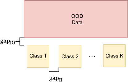
(a) ID and OOD Distributions

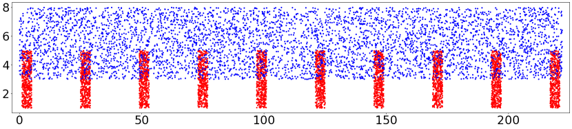
(b) Illustration of ID and OOD Data

Figure 2: ID and OOD distributions in Figure 1.

Configuration. The architecture of ID classifier is a four-layer FCNN. The number of neurons in hidden layers is set to $100$, and the number of neurons of output layer is set to $10$. These neurons use sigmoid activations. We use the Adam optimizer [82] to optimize the network’s parameters (with the $\ell_{2}$ loss). The learning rate is set to $0.001$, and the max number of training iterations is set to $10,000$. Within each iteration, we use full batch to update the network’s parameters. ${\rm gap}_{\rm II}$ is set to $20$ in our experiments. In Figure 1b, ${\rm gap}_{\rm IO}=-2$ (the overlap exists, see Figure 2), and in Figure 1c, ${\rm gap}_{\rm IO}=100$ (no overlap).

OOD Detection Procedure. We first train an ID classifier with $n$ data drawn from the ID distribution. Then, according to [23], we apply the free-energy score to identify the OOD data and calculate the $\alpha$-risk (with the $0$-$1$ loss). We repeat the above detection procedure $20$ times and report the average $\alpha$-risk in Figure 1. Note that, following [23], we choose the threshold used by the free-energy method so that $95\%$ of ID data are correctly identified as the ID classes by the OOD detector.

Appendix D Notations

D.1 Main Notations and Their Descriptions

In this section, we summarize important notations in Table 1.

Table 1: Main notations and their descriptions.

Notation	Description
$\bullet$ Spaces and Labels
$d$ and $\mathcal{X}\subset\mathbb{R}^{d}$	the feature dimension of data point and feature space
$\mathcal{Y}$	ID label space $\{1,...,K\}$
$K+1$	$K+1$ represents the OOD labels
$\mathcal{Y}_{\rm all}$	$\mathcal{Y}\cup\{K+1\}$
$\bullet$ Distributions
$X_{\rm I}$, $X_{\rm O}$, $Y_{\rm I}$, $Y_{\rm O}$	ID feature, OOD feature, ID label, OOD label random variables
$D_{X_{\rm I}Y_{\rm I}}$, $D_{X_{\rm O}Y_{\rm O}}$	ID joint distribution and OOD joint distribution
$D_{XY}^{\alpha}$	$D_{XY}^{\alpha}=(1-\alpha)D_{X_{\rm I}Y_{\rm I}}+\alpha D_{X_{\rm O}Y_{\rm O}},~{}~{}\forall\alpha\in[0,1]$
$\pi^{\rm out}$	class-prior probability for OOD distribution
$D_{XY}$	$D_{XY}=(1-\pi^{\rm out})D_{X_{\rm I}Y_{\rm I}}+\pi^{\rm out}D_{X_{\rm O}Y_{\rm O}}$, called domain
$D_{X_{\rm I}},D_{X_{\rm O}},D_{X}$	marginal distributions for $D_{X_{\rm I}Y_{\rm I}}$, $D_{X_{\rm O}Y_{\rm O}}$ and $D_{XY}$, respectively
$\bullet$ Domain Spaces
$\mathscr{D}_{XY}$	domain space consisting of some domains
$\mathscr{D}_{XY}^{\rm all}$	total space
$\mathscr{D}_{XY}^{s}$	seperate space
$\mathscr{D}_{XY}^{D_{XY}}$	single-distribution space
$\mathscr{D}_{XY}^{F}$	finite-ID-distribution space
$\mathscr{D}_{XY}^{\mu,b}$	density-based space
$\bullet$ Loss Function, Function Spaces
$\ell(\cdot,\cdot)$	loss: $\mathcal{Y}_{\rm all}\times\mathcal{Y}_{\rm all}\rightarrow\mathbb{R}_{\geq 0}$: $\ell(y_{1},y_{2})=0$ if and only if $y_{1}=y_{2}$
$\mathcal{H}$	hypothesis space
$\mathcal{H}^{\rm in}$	ID hypothesis space
$\mathcal{H}^{\rm b}$	hypothesis space in binary classification
$\mathcal{F}_{l}$	scoring function space consisting some $l$ dimensional vector-valued functions
$\bullet$ Risks and Partial Risks
$R_{D}(h)$	risk corresponding to $D_{XY}$
$R_{D}^{\rm in}(h)$	partial risk corresponding to $D_{X_{\rm I}Y_{\rm I}}$
$R_{D}^{\rm out}(h)$	partial risk corresponding to $D_{X_{\rm O}Y_{\rm O}}$
$R_{D}^{\alpha}(h)$	$\alpha$-risk corresponding to $D_{XY}^{\alpha}$
$\bullet$ Fully-Connected Neural Networks
$\mathbf{q}$	a sequence $(l_{1},...,l_{g})$ to represent the architecture of FCNN
$\sigma$	activation function. In this paper, we use ReLU function
$\mathcal{F}_{\mathbf{q}}^{\sigma}$	FCNN-based scoring function space
$\mathcal{H}_{\mathbf{q}}^{\sigma}$	FCNN-based hypothesis space
$\mathbf{f}_{\mathbf{w},\mathbf{b}}$	FCNN-based scoring function, which is from $\mathcal{F}_{\mathbf{q}}^{\sigma}$
${h}_{\mathbf{w},\mathbf{b}}$	FCNN-based hypothesis function, which is from $\mathcal{H}_{\mathbf{q}}^{\sigma}$
$\bullet$ Score-based Hypothesis Space
$E$	scoring function
$\lambda$	threshold
$\mathcal{H}_{\mathbf{q},E}^{\sigma,\lambda}$	score-based hypothesis space—a binary classification space
${h}_{\mathbf{f},E}^{\lambda}$	score-based hypothesis function—a binary classifier

Given $\mathbf{f}=[f^{1},...,f^{l}]^{\top}$, for any $\mathbf{x}\in\mathcal{X}$,

$$\operatorname*{arg\,max}_{k\in\{1,...,l\}}f^{k}(\mathbf{x}):=\max\{k\in\{1,...,l\}:f^{k}(\mathbf{x})\geq f^{i}(\mathbf{x}),\forall i=1,...,l\},$$

where $f^{k}$ is the $k$-th coordinate of $\mathbf{f}$ and $f^{i}$ is the $i$-th coordinate of $\mathbf{f}$. The above definition about $\operatorname*{arg\,max}$ aims to overcome some special cases. For example, there exist ${k}_{1}$, ${k}_{2}$ ($k_{1}<k_{2}$) such that $f^{k_{1}}(\mathbf{x})=f^{k_{2}}(\mathbf{x})$ and $f^{k_{1}}(\mathbf{x})>f^{i}(\mathbf{x})$, $f^{k_{2}}(\mathbf{x})>f^{i}(\mathbf{x})$, $\forall i\in\{1,...,l\}{-}\{k_{1},k_{2}\}$. Then, according to the above definition, $k_{2}=\operatorname*{arg\,max}_{k\in\{1,...,l\}}f^{k}(\mathbf{x})$.

D.2 Realizability Assumption

Assumption 2 (Realizability Assumption).

A domain space $\mathscr{D}_{XY}$ and hypothesis space $\mathcal{H}$ satisfy the Realizability Assumption, if for each domain $D_{XY}\in\mathscr{D}_{XY}$, there exists at least one hypothesis function $h^{*}\in\mathcal{H}$ such that $R_{D}(h^{*})=0$.

D.3 Learnability and PAC learnability

Here we give a proof to show that Learnability given in Definition 1 and PAC learnability are equivalent.

First, we prove that Learnability concludes the PAC learnability.

According to Definition 1,

$$\mathbb{E}_{S\sim D^{n}_{X_{\rm I}Y_{\rm I}}}R_{D}(\mathbf{A}(S))\leq\inf_{h\in\mathcal{H}}R_{D}(h)+\epsilon_{\rm cons}(n),$$

which implies that

$$\mathbb{E}_{S\sim D^{n}_{X_{\rm I}Y_{\rm I}}}[R_{D}(\mathbf{A}(S))-\inf_{h\in\mathcal{H}}R_{D}(h)]\leq\epsilon_{\rm cons}(n).$$

Note that $R_{D}(\mathbf{A}(S))-\inf_{h\in\mathcal{H}}R_{D}(h)\geq 0$. Therefore, by Markov’s inequality, we have

$$\mathbb{P}(R_{D}(\mathbf{A}(S))-\inf_{h\in\mathcal{H}}R_{D}(h)<\epsilon)>1-\mathbb{E}_{S\sim D^{n}_{X_{\rm I}Y_{\rm I}}}[R_{D}(\mathbf{A}(S))-\inf_{h\in\mathcal{H}}R_{D}(h)]/\epsilon\geq 1-\epsilon_{\rm cons}(n)/\epsilon.$$

Because $\epsilon_{\rm cons}(n)$ is monotonically decreasing, we can find a smallest $m$ such that $\epsilon_{\rm cons}(m)\geq\epsilon\delta$ and $\epsilon_{\rm cons}(m-1)<\epsilon\delta$, for $\delta\in(0,1)$. We define that $m(\epsilon,\delta)=m$. Therefore, for any $\epsilon>0$ and $\delta\in(0,1)$, there exists a function $m(\epsilon,\delta)$ such that when $n>m(\epsilon,\delta)$, with the probability at least $1-\delta$, we have

$$R_{D}(\mathbf{A}(S))-\inf_{h\in\mathcal{H}}R_{D}(h)<\epsilon,$$

which is the definition of PAC learnability.

Second, we prove that the PAC learnability concludes Learnability.

PAC-learnability: for any $\epsilon>0$ and $0<\delta<1$, there exists a function $m(\epsilon,\delta)>0$ such that when the sample size $n>m(\epsilon,\delta)$, we have that with the probability at least $1-\delta>0$,

$$R_{D}(\mathbf{A}(S))-\inf_{h\in\mathcal{H}}R_{D}(h)\leq\epsilon.$$

Note that the loss $\ell$ defined in Section 2 has upper bound (because $\mathcal{Y}\cup\{K+1\}$ is a finite set). We assume the upper bound of $\ell$ is $M$. Hence, according to the definition of PAC-learnability, when the sample size $n>m(\epsilon,\delta)$, we have that

$$\mathbb{E}_{S}[R_{D}(\mathbf{A}(S))-\inf_{h\in\mathcal{H}}R_{D}(h)]\leq\epsilon(1-\delta)+2M\delta<\epsilon+2M\delta.$$

If we set $\delta=\epsilon$, then when the sample size $n>m(\epsilon,\epsilon)$, we have that

$$\mathbb{E}_{S}[R_{D}(\mathbf{A}(S))-\inf_{h\in\mathcal{H}}R_{D}(h)]<(2M+1)\epsilon,$$

this implies that

$$\lim_{n\rightarrow+\infty}\mathbb{E}_{S}[R_{D}(\mathbf{A}(S))-\inf_{h\in\mathcal{H}}R_{D}(h)]=0,$$

which implies the Learnability in Definition 1. We have completed this proof.

D.4 Explanations for Some Notations in Section 2

First, we explain the concept that $S\sim{D}_{X_{I}Y_{I}}^{n}$ in Eq. (2).

$S=\{(\mathbf{x}^{1},{y}^{1}),...,(\mathbf{x}^{n},{y}^{n})\}$ is training data drawn independent and identically distributed from $D_{X_{\rm I}Y_{\rm I}}$.

$D_{X_{\rm I}Y_{\rm I}}^{n}$ denotes the probability over $n$-tuples induced by applying $D_{X_{\rm I}Y_{\rm I}}$ to pick each element of the tuple independently of the other members of the tuple.

Because these samples are i.i.d. drawn $n$ times, researchers often use ”$S\sim D_{X_{\rm I}Y_{\rm I}}^{n}$” to represent a sample set $S$ (of size $n$) whose each element is drawn i.i.d. from $D_{X_{\rm I}Y_{\rm I}}$.

Second, we explain the concept ”$+$” in $(1-\pi^{\rm out})D_{X_{\rm I}}+\pi^{\rm out}D_{X_{\rm O}}$.

For convenience, let $P=(1-\pi^{\rm out})D_{X_{\rm I}}$ and $Q=\pi^{\rm out}D_{X_{\rm O}}$. It is clear that $P$ and $Q$ are measures. Then $P+Q$ is also a measure, which is defined as follows: for any measurable set $A\subset\mathcal{X}$, we have

$$(P+Q)(A)=P(A)+Q(A).$$

For example, when $P$ and $Q$ are discrete measures, then $P+Q$ is also discrete measure: for any $\mathbf{x}\in\mathcal{X}$,

$$(P+Q)(\mathbf{x})=P(\mathbf{x})+Q(\mathbf{x}).$$

When $P$ and $Q$ are continuous measures with density functions $f$ and $g$, then $P+Q$ is also continuous measure with density function $f+g$: for any measurable $A\subset\mathcal{X}$,

$$P(A)=\int_{A}f(\mathbf{x}){\rm d}\mathbf{x},~{}~{}~{}Q(A)=\int_{A}g(\mathbf{x}){\rm d}\mathbf{x},$$

then

$$(P+Q)(A)=\int_{A}f(\mathbf{x})+g(\mathbf{x}){\rm d}\mathbf{x}.$$

Third, we explain the concept $\mathbb{E}_{(\mathbf{x},y)\sim D_{XY}}\ell({h}(\mathbf{x}),{y}).$

The concept $\mathbb{E}_{(\mathbf{x},y)\sim D_{XY}}\ell({h}(\mathbf{x}),{y})$ can be computed as follows:

$$\mathbb{E}_{(\mathbf{x},y)\sim D_{XY}}\ell({h}(\mathbf{x}),{y})=\int_{\mathcal{X}\times\mathcal{Y}_{\rm all}}\ell({h}(\mathbf{x}),{y}){\rm d}D_{XY}(\mathbf{x},y).$$

For example, when $D_{XY}$ is a finite discrete distribution: let $\mathcal{Z}=\{(\mathbf{x}^{1},y^{1}),...,(\mathbf{x}^{m},y^{m})\}$ be the support set of $D_{XY}$, and assume that $a^{i}$ is the probability for $(\mathbf{x}^{i},y^{i})$, i.e., $a^{i}=D_{XY}(\mathbf{x}^{i},y^{i})$. Then

$$\begin{split}\mathbb{E}_{(\mathbf{x},y)\sim D_{XY}}\ell({h}(\mathbf{x}),{y})&=\int_{\mathcal{X}\times\mathcal{Y}_{\rm all}}\ell({h}(\mathbf{x}),{y}){\rm d}D_{XY}(\mathbf{x},y)\\ &=\frac{1}{m}\sum_{i=1}^{m}a^{i}\ell({h}(\mathbf{x}^{i}),{y}^{i}).\end{split}$$

When $D_{X}$ is a continuous distribution with density $f$, and $D_{Y|X}(Y=k|X=\mathbf{x})$ ($k$-th class-conditional distribution for $\mathbf{x}$) is $a^{k}(\mathbf{x})$, then

$$\begin{split}\mathbb{E}_{(\mathbf{x},y)\sim D_{XY}}\ell({h}(\mathbf{x}),{y})&=\int_{\mathcal{X}\times\mathcal{Y}_{\rm all}}\ell({h}(\mathbf{x}),{y}){\rm d}D_{XY}(\mathbf{x},y)\\ &=\int_{\mathcal{X}}\sum_{k=1}^{K+1}\ell({h}(\mathbf{x}),k)f(\mathbf{x})a^{k}(\mathbf{x}){\rm d}\mathbf{x},\end{split}$$

where $D_{Y|X}(Y=k|X=\mathbf{x})$ is the $k$-th class-conditional distribution.

Appendix E Proof of Theorem 1

See 1

Proof of Theorem 1..

 

Proof of the First Result.

To prove that $\mathscr{D}_{XY}^{\prime}$ is a priori-unknown space, we need to show that for any $D_{XY}^{\alpha^{\prime}}\in\mathscr{D}_{XY}^{\prime}$, then $D_{XY}^{\alpha}\in\mathscr{D}_{XY}^{\prime}$ for any $\alpha\in[0,1)$.

According to the definition of $\mathscr{D}_{XY}^{\prime}$, for any $D_{XY}^{\alpha^{\prime}}\in\mathscr{D}_{XY}^{\prime}$, we can find a domain $D_{XY}\in\mathscr{D}_{XY}$, which can be written as $D_{XY}=(1-\pi^{\rm out})D_{X_{\rm I}Y_{\rm I}}+\pi^{\rm out}D_{X_{\rm O}Y_{\rm O}}$ (here $\pi^{\rm out}\in[0,1)$) such that

$$D_{XY}^{\alpha^{\prime}}=(1-\alpha^{\prime})D_{X_{\rm I}Y_{\rm I}}+\alpha^{\prime}D_{X_{\rm O}Y_{\rm O}}.$$

Note that $D_{XY}^{\alpha}=(1-\alpha)D_{X_{\rm I}Y_{\rm I}}+\alpha D_{X_{\rm O}Y_{\rm O}}$.

Therefore, based on the definition of $\mathscr{D}_{XY}^{\prime}$, for any $\alpha\in[0,1)$, $D_{XY}^{\alpha}\in\mathscr{D}_{XY}^{\prime}$, which implies that $\mathscr{D}_{XY}^{\prime}$ is a prior-known space. Additionally, for any $D_{XY}\in\mathscr{D}_{XY}$, we can rewrite $D_{XY}$ as $D_{XY}^{\pi_{\rm out}}$, thus $D_{XY}=D_{XY}^{\pi_{\rm out}}\in\mathscr{D}_{XY}^{\prime}$, which implies that $\mathscr{D}_{XY}\subset\mathscr{D}_{XY}^{\prime}$.

Proof of the Second Result.

First, we prove that Definition 1 concludes Definition 2, if $\mathscr{D}_{XY}$ is a prior-unknown space:

The domain space $\mathscr{D}_{XY}$ is a priori-unknown space, and OOD detection is learnable in $\mathscr{D}_{XY}$ for $\mathcal{H}$. $~{}~{}~{}~{}~{}~{}~{}~{}~{}~{}~{}~{}~{}~{}~{}~{}~{}~{}~{}~{}~{}~{}~{}~{}~{}~{}~{}~{}~{}~{}~{}~{}~{}~{}~{}~{}~{}~{}~{}~{}~{}~{}~{}~{}~{}~{}~{}~{}~{}~{}~{}~{}~{}~{}~{}~{}~{}~{}~{}~{}~{}~{}~{}~{}~{}~{}~{}~{}~{}~{}~{}~{}~{}~{}~{}~{}~{}~{}{\Huge\Downarrow}$ OOD detection is strongly learnable in $\mathscr{D}_{XY}$ for $\mathcal{H}$: there exist an algorithm $\mathbf{A}:\cup_{n=1}^{+\infty}(\mathcal{X}\times\mathcal{Y})^{n}\rightarrow\mathcal{H}$, and a monotonically decreasing sequence $\epsilon(n)$, such that $\epsilon(n)\rightarrow 0$, as $n\rightarrow+\infty$ $$\begin{split}\mathbb{E}_{S\sim D^{n}_{X_{\rm I}Y_{\rm I}}}\big{[}R^{\alpha}_{D}(\mathbf{A}(S))&-\inf_{h\in\mathcal{H}}R^{\alpha}_{D}(h)\big{]}\leq\epsilon(n),~{}~{}~{}\forall\alpha\in[0,1],~{}\forall D_{XY}\in\mathscr{D}_{XY}.\end{split}$$

In the priori-unknown space, for any $D_{XY}\in\mathscr{D}_{XY}$, we have that for any $\alpha\in[0,1)$,

$$D_{XY}^{\alpha}=(1-\alpha)D_{X_{\rm I}Y_{\rm I}}+\alpha D_{X_{\rm O}Y_{\rm O}}\in\mathscr{D}_{XY}.$$

Then, according to the definition of learnability of OOD detection, we have an algorithm $\mathbf{A}$ and a monotonically decreasing sequence $\epsilon_{\rm cons}(n)\rightarrow 0$, as $n\rightarrow+\infty$, such that for any $\alpha\in[0,1)$,

$$\mathbb{E}_{S\sim D^{n}_{X_{\rm I}Y_{\rm I}}}R_{D^{\alpha}}(\mathbf{A}(S))\leq\inf_{h\in\mathcal{H}}R_{D^{\alpha}}(h)+\epsilon_{\rm cons}(n),~{}~{}(\textnormal{{by~{}the~{}property~{}of~{}priori}-{\rm unknown~{}space}})$$

where

$$R_{D^{\alpha}}(\mathbf{A}(S))=\int_{\mathcal{X}\times\mathcal{Y}_{\rm all}}\ell(\mathbf{A}(S)(\mathbf{x}),y){\rm d}D^{\alpha}_{XY}(\mathbf{x},y),~{}~{}~{}R_{D^{\alpha}}(h)=\int_{\mathcal{X}\times\mathcal{Y}_{\rm all}}\ell(h(\mathbf{x}),y){\rm d}D^{\alpha}_{XY}(\mathbf{x},y).$$

Since $R_{D^{\alpha}}(\mathbf{A}(S))=R_{D}^{\alpha}(\mathbf{A}(S))$ and $R_{D^{\alpha}}(h)=R_{D}^{\alpha}(h)$, we have that

$$\mathbb{E}_{S\sim D^{n}_{X_{\rm I}Y_{\rm I}}}R_{D}^{\alpha}(\mathbf{A}(S))\leq\inf_{h\in\mathcal{H}}R_{D}^{\alpha}(h)+\epsilon_{\rm cons}(n),~{}~{}~{}\forall\alpha\in[0,1).$$ (9)

Next, we consider the case that $\alpha=1$. Note that

$$\liminf_{\alpha\rightarrow 1}\inf_{h\in\mathcal{H}}R_{D}^{\alpha}(h)\geq\liminf_{\alpha\rightarrow 1}\alpha\inf_{h\in\mathcal{H}}R_{D}^{\rm out}(h)=\inf_{h\in\mathcal{H}}R_{D}^{\rm out}(h).$$ (10)

Then, we assume that $h_{\epsilon}\in\mathcal{H}$ satisfies that

$$R_{D}^{\rm out}(h_{\epsilon})-\inf_{h\in\mathcal{H}}R_{D}^{\rm out}(h)\leq\epsilon.$$

It is obvious that

$$R_{D}^{\alpha}(h_{\epsilon})\geq\inf_{h\in\mathcal{H}}R_{D}^{\alpha}(h).$$

Let $\alpha\rightarrow 1$. Then, for any $\epsilon>0$,

$$R_{D}^{\rm out}(h_{\epsilon})=\lim_{\alpha\rightarrow 1}R_{D}^{\alpha}(h_{\epsilon})=\limsup_{\alpha\rightarrow 1}R_{D}^{\alpha}(h_{\epsilon})\geq\limsup_{\alpha\rightarrow 1}\inf_{h\in\mathcal{H}}R_{D}^{\alpha}(h),$$

which implies that

$$\inf_{h\in\mathcal{H}}R_{D}^{\rm out}(h)=\lim_{\epsilon\rightarrow 0}R_{D}^{\rm out}(h_{\epsilon})\geq\lim_{\epsilon\rightarrow 0}\limsup_{\alpha\rightarrow 1}\inf_{h\in\mathcal{H}}R_{D}^{\alpha}(h)=\limsup_{\alpha\rightarrow 1}\inf_{h\in\mathcal{H}}R_{D}^{\alpha}(h).$$ (11)

Combining Eq. (10) with Eq. (11), we have

$$\inf_{h\in\mathcal{H}}R_{D}^{\rm out}(h)=\limsup_{\alpha\rightarrow 1}\inf_{h\in\mathcal{H}}R_{D}^{\alpha}(h)=\liminf_{\alpha\rightarrow 1}\inf_{h\in\mathcal{H}}R_{D}^{\alpha}(h),$$ (12)

which implies that

$$\inf_{h\in\mathcal{H}}R_{D}^{\rm out}(h)=\lim_{\alpha\rightarrow 1}\inf_{h\in\mathcal{H}}R_{D}^{\alpha}(h).$$ (13)

Note that

$$\mathbb{E}_{S\sim D^{n}_{X_{\rm I}Y_{\rm I}}}R_{D}^{\alpha}(\mathbf{A}(S))=(1-\alpha)\mathbb{E}_{S\sim D^{n}_{X_{\rm I}Y_{\rm I}}}R_{D}^{\rm in}(\mathbf{A}(S))+\alpha\mathbb{E}_{S\sim D^{n}_{X_{\rm I}Y_{\rm I}}}R_{D}^{\rm out}(\mathbf{A}(S)).$$

Hence, Lebesgue’s Dominated Convergence Theorem [36] implies that

$$\lim_{\alpha\rightarrow 1}\mathbb{E}_{S\sim D^{n}_{X_{\rm I}Y_{\rm I}}}R_{D}^{\alpha}(\mathbf{A}(S))=\mathbb{E}_{S\sim D^{n}_{X_{\rm I}Y_{\rm I}}}R_{D}^{\rm out}(\mathbf{A}(S)).$$ (14)

Using Eq. (9), we have that

$$\lim_{\alpha\rightarrow 1}\mathbb{E}_{S\sim D^{n}_{X_{\rm I}Y_{\rm I}}}R_{D}^{\alpha}(\mathbf{A}(S))\leq\lim_{\alpha\rightarrow 1}\inf_{h\in\mathcal{H}}R_{D}^{\alpha}(h)+\epsilon_{\rm cons}(n).$$ (15)

Combining Eq. (13), Eq. (14) with Eq. (15), we obtain that

$$\mathbb{E}_{S\sim D^{n}_{X_{\rm I}Y_{\rm I}}}R_{D}^{\rm out}(\mathbf{A}(S))\leq\inf_{h\in\mathcal{H}}R_{D}^{\rm out}(h)+\epsilon_{\rm cons}(n).$$

Since $R_{D}^{\rm out}(\mathbf{A}(S))=R_{D}^{1}(\mathbf{A}(S))$ and $R_{D}^{\rm out}(h)=R_{D}^{1}(h)$, we obtain that

$$\mathbb{E}_{S\sim D^{n}_{X_{\rm I}Y_{\rm I}}}R_{D}^{1}(\mathbf{A}(S))\leq\inf_{h\in\mathcal{H}}R_{D}^{1}(h)+\epsilon_{\rm cons}(n).$$ (16)

Combining Eq. (9) and Eq. (16), we have proven that: if the domain space $\mathscr{D}_{XY}$ is a priori-unknown space, then OOD detection is learnable in $\mathscr{D}_{XY}$ for $\mathcal{H}$.
$~{}~{}~{}~{}~{}~{}~{}~{}~{}~{}~{}~{}~{}~{}~{}~{}~{}~{}~{}~{}~{}~{}~{}~{}~{}~{}~{}~{}~{}~{}~{}~{}~{}~{}~{}~{}~{}~{}~{}~{}~{}~{}~{}~{}~{}~{}~{}~{}~{}~{}~{}~{}~{}~{}~{}~{}~{}~{}~{}~{}~{}~{}~{}~{}~{}~{}~{}~{}~{}~{}~{}~{}~{}~{}~{}~{}~{}~{}~{}{\Huge\Downarrow}$
OOD detection is strongly learnable in $\mathscr{D}_{XY}$ for $\mathcal{H}$: there exist an algorithm $\mathbf{A}:\cup_{n=1}^{+\infty}(\mathcal{X}\times\mathcal{Y})^{n}\rightarrow\mathcal{H}$, and a monotonically decreasing sequence $\epsilon(n)$, such that $\epsilon(n)\rightarrow 0$, as $n\rightarrow+\infty$,

$$\begin{split}\mathbb{E}_{S\sim D^{n}_{X_{\rm I}Y_{\rm I}}}R^{\alpha}_{D}(\mathbf{A}(S))&\leq\inf_{h\in\mathcal{H}}R^{\alpha}_{D}(h)+\epsilon(n),~{}~{}~{}\forall\alpha\in[0,1],~{}\forall D_{XY}\in\mathscr{D}_{XY}.\end{split}$$

Second, we prove that Definition 2 concludes Definition 1:
OOD detection is strongly learnable in $\mathscr{D}_{XY}$ for $\mathcal{H}$: there exist an algorithm $\mathbf{A}:\cup_{n=1}^{+\infty}(\mathcal{X}\times\mathcal{Y})^{n}\rightarrow\mathcal{H}$, and a monotonically decreasing sequence $\epsilon(n)$, such that $\epsilon(n)\rightarrow 0$, as $n\rightarrow+\infty$, $$\begin{split}\mathbb{E}_{S\sim D^{n}_{X_{\rm I}Y_{\rm I}}}\big{[}R^{\alpha}_{D}(\mathbf{A}(S))&-\inf_{h\in\mathcal{H}}R^{\alpha}_{D}(h)\big{]}\leq\epsilon(n),~{}~{}~{}\forall\alpha\in[0,1],~{}\forall D_{XY}\in\mathscr{D}_{XY}.\end{split}$$ $~{}~{}~{}~{}~{}~{}~{}~{}~{}~{}~{}~{}~{}~{}~{}~{}~{}~{}~{}~{}~{}~{}~{}~{}~{}~{}~{}~{}~{}~{}~{}~{}~{}~{}~{}~{}~{}~{}~{}~{}~{}~{}~{}~{}~{}~{}~{}~{}~{}~{}~{}~{}~{}~{}~{}~{}~{}~{}~{}~{}~{}~{}~{}~{}~{}~{}~{}~{}~{}~{}~{}~{}~{}~{}~{}~{}~{}~{}~{}~{}{\Huge\Downarrow}$                                                OOD detection is learnable in $\mathscr{D}_{XY}$ for $\mathcal{H}$.

If we set $\alpha=\pi^{\rm out}$, then $\mathbb{E}_{S\sim D^{n}_{X_{\rm I}Y_{\rm I}}}R^{\alpha}_{D}(\mathbf{A}(S))\leq\inf_{h\in\mathcal{H}}R^{\alpha}_{D}(h)+\epsilon(n)$ implies that

$$\begin{split}\mathbb{E}_{S\sim D^{n}_{X_{\rm I}Y_{\rm I}}}R_{D}(\mathbf{A}(S))\leq\inf_{h\in\mathcal{H}}R_{D}(h)+\epsilon(n),\end{split}$$

which means that OOD detection is learnable in $\mathscr{D}_{XY}$ for $\mathcal{H}$. We have completed this proof.

Proof of the Third Result.

The third result is a simple conclusion of the second result. Hence, we omit it. ∎

Appendix F Proof of Theorem 2

Before introducing the proof of Theorem 2, we extend Condition 1 to a general version (Condition 4). Then, Lemma 1 proves that Conditions 1 and 4 are the necessary conditions for the learnability of OOD detection. First, we provide the details of Condition 4.

Let $\Delta_{l}^{\rm o}=\{(\lambda_{1},...,\lambda_{l}):\sum_{j=1}^{l}\lambda_{j}<1~{}{\rm and}~{}\lambda_{j}\geq 0,\forall j=1,...,l\}$, where $l$ is a positive integer. Next, we introduce an important definition as follows:

Definition 6 (OOD Convex Decomposition and Convex Domain).

Given any domain $D_{XY}\in\mathscr{D}_{XY}$, we say joint distributions $Q_{1},...,Q_{l}$, which are defined over $\mathcal{X}\times\{K+1\}$, are the OOD convex decomposition for $D_{XY}$, if

$$D_{XY}=(1-\sum_{j=1}^{l}\lambda_{j})D_{X_{\rm I}Y_{\rm I}}+\sum_{j=1}^{l}\lambda_{j}Q_{j},$$

for some $(\lambda_{1},...,\lambda_{l})\in\Delta_{l}^{\rm o}$. We also say domain $D_{XY}\in\mathscr{D}_{XY}$ is an OOD convex domain corresponding to OOD convex decomposition $Q_{1},...,Q_{l}$, if for any $(\alpha_{1},...,\alpha_{l})\in\Delta_{l}^{\rm o}$,

$$(1-\sum_{j=1}^{l}\alpha_{j})D_{X_{\rm I}Y_{\rm I}}+\sum_{j=1}^{l}\alpha_{j}Q_{j}\in\mathscr{D}_{XY}.$$

We extend the linear condition (Condition 1) to a multi-linear scenario.

Condition 4 (Multi-linear Condition).

For each OOD convex domain $D_{XY}\in\mathscr{D}_{XY}$ corresponding to OOD convex decomposition $Q_{1},...,Q_{l}$, the following function

$$f_{D,Q}(\alpha_{1},...,\alpha_{l}):=\inf_{h\in\mathcal{H}}\Big{(}(1-\sum_{j=1}^{l}\alpha_{j})R_{D}^{\rm in}(h)+\sum_{j=1}^{l}\alpha_{j}R_{Q_{j}}(h)\Big{)},~{}~{}~{}\forall(\alpha_{1},...,\alpha_{l})\in\Delta_{l}^{\rm o}$$

satisfies that

$$f_{D,Q}(\alpha_{1},...,\alpha_{l})=(1-\sum_{j=1}^{l}\alpha_{j})f_{D,Q}(\mathbf{0})+\sum_{j=1}^{l}\alpha_{j}f_{D,Q}({\bm{\alpha}}_{j}),$$

where $\mathbf{0}$ is the $1\times l$ vector, whose elements are $0$, and ${\bm{\alpha}}_{j}$ is the $1\times l$ vector, whose $j$-th element is $1$ and other elements are $0$.

When $l=1$ and the domain space $\mathscr{D}_{XY}$ is a priori-unknown space, Condition 4 degenerates into Condition 1. Lemma 1 shows that Condition 4 is necessary for the learnability of OOD detection.

Lemma 1.

Given a priori-unknown space $\mathscr{D}_{XY}$ and a hypothesis space $\mathcal{H}$, if OOD detection is learnable in $\mathscr{D}_{XY}$ for $\mathcal{H}$, then Conditions 1 and 4 hold.

Proof of Lemma 1.

 

Since Condition 1 is a special case of Condition 4, we only need to prove that Condition 4 holds.

For any OOD convex domain $D_{XY}\in\mathscr{D}_{XY}$ corresponding to OOD convex decomposition $Q_{1},...,Q_{l}$, and any $(\alpha_{1},...,\alpha_{l})\in\Delta_{l}^{\rm o}$, we set

$$Q^{\bm{\alpha}}=\frac{1}{\sum_{i=1}^{l}\alpha_{i}}\sum_{j=1}^{l}\alpha_{j}Q_{j}.$$

Then, we define

$$D_{XY}^{\bm{\alpha}}=(1-\sum_{i=1}^{l}\alpha_{i})D_{X_{\rm I}Y_{\rm I}}+(\sum_{i=1}^{l}\alpha_{i})Q^{\bm{\alpha}},~{}\textnormal{which~{}belongs~{}to~{}}\mathscr{D}_{XY}.$$

Let

$$R^{\bm{\alpha}}_{D}(h)=\int_{\mathcal{X}\times\mathcal{Y}_{\rm all}}\ell(h(\mathbf{x}),y){\rm d}D_{XY}^{\bm{\alpha}}(\mathbf{x},y).$$

Since OOD detection is learnable in $\mathscr{D}_{XY}$ for $\mathcal{H}$, there exist an algorithm $\mathbf{A}:\cup_{n=1}^{+\infty}(\mathcal{X}\times\mathcal{Y})^{n}\rightarrow\mathcal{H}$, and a monotonically decreasing sequence $\epsilon(n)$, such that $\epsilon(n)\rightarrow 0$, as $n\rightarrow+\infty$, and

$$0\leq\mathbb{E}_{S\sim D^{n}_{X_{\rm I}Y_{\rm I}}}R^{\bm{\alpha}}_{D}(\mathbf{A}(S))-\inf_{h\in\mathcal{H}}R^{\bm{\alpha}}_{D}(h)\leq\epsilon(n).$$

Note that

$$\begin{split}&\mathbb{E}_{S\sim D^{n}_{X_{\rm I}Y_{\rm I}}}R^{\bm{\alpha}}_{D}(\mathbf{A}(S))=(1-\sum_{j=1}^{l}\alpha_{j})\mathbb{E}_{S\sim D^{n}_{X_{\rm I}Y_{\rm I}}}R^{\rm in}_{D}(\mathbf{A}(S))+\sum_{j=1}^{l}\alpha_{j}\mathbb{E}_{S\sim D^{n}_{X_{\rm I}Y_{\rm I}}}R_{Q_{j}}(\mathbf{A}(S)),\end{split}$$

and

$$\inf_{h\in\mathcal{H}}R^{\bm{\alpha}}_{D}(h)=f_{D,Q}(\alpha_{1},...,\alpha_{l}),$$

where

$$R_{Q_{j}}(\mathbf{A}(S))=\int_{\mathcal{X}\times\{K+1\}}\ell(\mathbf{A}(S)(\mathbf{x}),y){\rm d}Q_{j}(\mathbf{x},y).$$

Therefore, we have that for any $(\alpha_{1},...,\alpha_{l})\in\Delta_{l}^{\rm o}$,

$$\begin{split}&\big{|}(1-\sum_{j=1}^{l}\alpha_{j})\mathbb{E}_{S\sim D^{n}_{X_{\rm I}Y_{\rm I}}}R^{\rm in}_{D}(\mathbf{A}(S))+\sum_{j=1}^{l}\alpha_{j}\mathbb{E}_{S\sim D^{n}_{X_{\rm I}Y_{\rm I}}}R_{Q_{j}}(\mathbf{A}(S))-f_{D,Q}(\alpha_{1},...,\alpha_{l})\big{|}\leq\epsilon(n).\end{split}$$ (17)

Let

$$g_{n}(\alpha_{1},...,\alpha_{l})=(1-\sum_{j=1}^{l}\alpha_{j})\mathbb{E}_{S\sim D^{n}_{X_{\rm I}Y_{\rm I}}}R^{\rm in}_{D}(\mathbf{A}(S))+\sum_{j=1}^{l}\alpha_{j}\mathbb{E}_{S\sim D^{n}_{X_{\rm I}Y_{\rm I}}}R_{Q_{j}}(\mathbf{A}(S)).$$

Note that Eq. (17) implies that

$$\begin{split}\lim_{n\rightarrow+\infty}g_{n}(\alpha_{1},...,\alpha_{l})&=f_{D,Q}(\alpha_{1},...,\alpha_{l}),~{}~{}\forall(\alpha_{1},...,\alpha_{l})\in\Delta_{l}^{\rm o},\\ \lim_{n\rightarrow+\infty}g_{n}(\mathbf{0})&=f_{D,Q}(\mathbf{0}).\end{split}$$ (18)

Step 1. Since ${\bm{\alpha}}_{j}\notin\Delta_{l}^{\rm o}$, we need to prove that

$$\lim_{n\rightarrow+\infty}\mathbb{E}_{S\sim D^{n}_{X_{\rm I}Y_{\rm I}}}R_{Q_{j}}(\mathbf{A}(S))=f({\bm{\alpha}}_{j}),\textit{i.e.},\lim_{n\rightarrow+\infty}g_{n}({\bm{\alpha}}_{j})=f({\bm{\alpha}}_{j}),$$ (19)

where ${\bm{\alpha}}_{j}$ is the $1\times l$ vector, whose $j$-th element is $1$ and other elements are $0$.

Let $\tilde{D}_{XY}=0.5*D_{X_{\rm I}Y_{\rm I}}+0.5*Q_{j}$. The second result of Theorem 1 implies that

$$\begin{split}\mathbb{E}_{S\sim D^{n}_{X_{\rm I}Y_{\rm I}}}R^{\rm out}_{\tilde{D}}(\mathbf{A}(S))\leq\inf_{h\in\mathcal{H}}R^{\rm out}_{\tilde{D}}(h)+\epsilon(n).\end{split}$$

Since $R^{\rm out}_{\tilde{D}}(\mathbf{A}(S))=R_{Q_{j}}(\mathbf{A}(S))$ and $R^{\rm out}_{\tilde{D}}(h)=R_{Q_{j}}(h)$,

$$\mathbb{E}_{S\sim D^{n}_{X_{\rm I}Y_{\rm I}}}R_{Q_{j}}(\mathbf{A}(S))\leq\inf_{h\in\mathcal{H}}R_{Q_{j}}(h)+\epsilon(n).$$

Note that $\inf_{h\in\mathcal{H}}R_{Q_{j}}(h)\leq\mathbb{E}_{S\sim D^{n}_{X_{\rm I}Y_{\rm I}}}R_{Q_{j}}(\mathbf{A}(S))$. We have

$$0\leq\mathbb{E}_{S\sim D^{n}_{X_{\rm I}Y_{\rm I}}}R_{Q_{j}}(\mathbf{A}(S))-\inf_{h\in\mathcal{H}}R_{Q_{j}}(h)\leq\epsilon(n).$$ (20)

Eq. (20) implies that

$$\lim_{n\rightarrow+\infty}\mathbb{E}_{S\sim D^{n}_{X_{\rm I}Y_{\rm I}}}R_{Q_{j}}(\mathbf{A}(S))=\inf_{h\in\mathcal{H}}R_{Q_{j}}(h).$$ (21)

We note that $\inf_{h\in\mathcal{H}}R_{Q_{j}}(h)=f_{D,Q}({\bm{\alpha}}_{j})$. Therefore,

$$\lim_{n\rightarrow+\infty}\mathbb{E}_{S\sim D^{n}_{X_{\rm I}Y_{\rm I}}}R_{Q_{j}}(\mathbf{A}(S))=f_{D,Q}({\bm{\alpha}}_{j}),~{}\textit{i.e.},\lim_{n\rightarrow+\infty}g_{n}({\bm{\alpha}}_{j})=f({\bm{\alpha}}_{j}).$$ (22)

Step 2. It is easy to check that for any $(\alpha_{1},...,\alpha_{l})\in\Delta_{l}^{\rm o}$,

$$\begin{split}\lim_{n\rightarrow+\infty}g_{n}(\alpha_{1},...,\alpha_{l})&=\lim_{n\rightarrow+\infty}\big{(}(1-\sum_{j=1}^{l}\alpha_{j})g_{n}(\mathbf{0})+\sum_{j=1}^{l}\alpha_{j}g_{n}({\bm{\alpha}}_{j})\big{)}\\ &=(1-\sum_{j=1}^{l}\alpha_{j})\lim_{n\rightarrow+\infty}g_{n}(\mathbf{0})+\sum_{j=1}^{l}\alpha_{j}\lim_{n\rightarrow+\infty}g_{n}({\bm{\alpha}}_{j}).\end{split}$$ (23)

According to Eq. (18) and Eq. (22), we have

$$\begin{split}&\lim_{n\rightarrow+\infty}g_{n}(\alpha_{1},...,\alpha_{l})=f_{D,Q}(\alpha_{1},...,\alpha_{l}),~{}~{}\forall(\alpha_{1},...,\alpha_{l})\in\Delta_{l}^{\rm o},\\ &\lim_{n\rightarrow+\infty}g_{n}(\mathbf{0})=f_{D,Q}(\mathbf{0}),\\ &\lim_{n\rightarrow+\infty}g_{n}({\bm{\alpha}}_{j})=f({\bm{\alpha}}_{j}),\end{split}$$ (24)

Combining Eq. (24) with Eq. (23), we complete the proof. ∎

Lemma 2.

$$\inf_{h\in\mathcal{H}}R_{D}^{\alpha}(h)=(1-\alpha)\inf_{h\in\mathcal{H}}R_{D}^{\rm in}(h)+\alpha\inf_{h\in\mathcal{H}}R_{D}^{\rm out}(h),~{}\forall\alpha\in[0,1),$$

if and only if for any $\epsilon>0$,

$$\{h^{\prime}\in\mathcal{H}:R_{D}^{\rm in}(h^{\prime})\leq\inf_{h\in\mathcal{H}}R_{D}^{\rm in}(h)+2\epsilon\}\cap\{h^{\prime}\in\mathcal{H}:R_{D}^{\rm out}(h^{\prime})\leq\inf_{h\in\mathcal{H}}R_{D}^{\rm out}(h)+2\epsilon\}\neq\emptyset.$$

Proof of Lemma 2.

For the sake of convenience, we set $f_{D}(\alpha)=\inf_{h\in\mathcal{H}}R_{D}^{\alpha}(h)$, for any $\alpha\in[0,1]$.

First, we prove that $f_{D}(\alpha)=(1-\alpha)f_{D}(0)+\alpha f_{D}(1)$,  $\forall\alpha\in[0,1)$ implies

$$\{h^{\prime}\in\mathcal{H}:R_{D}^{\rm in}(h^{\prime})\leq\inf_{h\in\mathcal{H}}R_{D}^{\rm in}(h)+2\epsilon\}\cap\{h^{\prime}\in\mathcal{H}:R_{D}^{\rm out}(h^{\prime})\leq\inf_{h\in\mathcal{H}}R_{D}^{\rm out}(h)+2\epsilon\}\neq\emptyset.$$

For any $\epsilon>0$ and $0\leq\alpha<1$, we can find $h_{\epsilon}^{\alpha}\in\mathcal{H}$ satisfying that

$$R_{D}^{\alpha}(h_{\epsilon}^{\alpha})\leq\inf_{h\in\mathcal{H}}R_{D}^{\alpha}(h)+\epsilon.$$

Note that

$$\inf_{h\in\mathcal{H}}R_{D}^{\alpha}(h)=\inf_{h\in\mathcal{H}}\Big{(}(1-\alpha)R_{D}^{\rm in}(h)+\alpha R_{D}^{\rm out}(h)\Big{)}\geq(1-\alpha)\inf_{h\in\mathcal{H}}R_{D}^{\rm in}(h)+\alpha\inf_{h\in\mathcal{H}}R_{D}^{\rm out}(h).$$

Therefore,

$$(1-\alpha)\inf_{h\in\mathcal{H}}R_{D}^{\rm in}(h)+\alpha\inf_{h\in\mathcal{H}}R_{D}^{\rm out}(h)\leq\inf_{h\in\mathcal{H}}R_{D}^{\alpha}(h)\leq R_{D}^{\alpha}(h_{\epsilon}^{\alpha})\leq\inf_{h\in\mathcal{H}}R_{D}^{\alpha}(h)+\epsilon.$$ (25)

Note that $f_{D}(\alpha)=(1-\alpha)f_{D}(0)+\alpha f_{D}(1),\forall\alpha\in[0,1)$, i.e.,

$$\inf_{h\in\mathcal{H}}R_{D}^{\alpha}(h)=(1-\alpha)\inf_{h\in\mathcal{H}}R_{D}^{\rm in}(h)+\alpha\inf_{h\in\mathcal{H}}R_{D}^{\rm out}(h),\forall\alpha\in[0,1).$$ (26)

Using Eqs. (25) and (26), we have that for any $0\leq\alpha<1$,

$$\epsilon\geq\big{|}R^{\alpha}_{D}(h_{\epsilon}^{\alpha})-\inf_{h\in\mathcal{H}}R_{D}^{\alpha}(h)\big{|}=\big{|}(1-\alpha)\big{(}R_{D}^{\rm in}(h_{\epsilon}^{\alpha})-\inf_{h\in\mathcal{H}}R_{D}^{\rm in}(h)\big{)}+\alpha\big{(}R_{D}^{\rm out}(h_{\epsilon}^{\alpha})-\inf_{h\in\mathcal{H}}R_{D}^{\rm out}(h)\big{)}\big{|}.$$ (27)

Since $R_{D}^{\rm out}(h_{\epsilon}^{\alpha})-\inf_{h\in\mathcal{H}}R_{D}^{\rm out}(h)\geq 0$ and $R_{D}^{\rm in}(h_{\epsilon}^{\alpha})-\inf_{h\in\mathcal{H}}R_{D}^{\rm in}(h)\geq 0$, Eq. (27) implies that: for any $0<\alpha<1$,

$$\begin{split}&R_{D}^{\rm in}(h_{\epsilon}^{\alpha})\leq\inf_{h\in\mathcal{H}}R_{D}^{\rm in}(h)+\epsilon/(1-\alpha),\\ &R_{D}^{\rm out}(h_{\epsilon}^{\alpha})\leq\inf_{h\in\mathcal{H}}R_{D}^{\rm out}(h)+\epsilon/\alpha.\end{split}$$

Therefore,

$$h_{\epsilon}^{\alpha}\in\{h^{\prime}\in\mathcal{H}:R_{D}^{\rm in}(h^{\prime})\leq\inf_{h\in\mathcal{H}}R_{D}^{\rm in}(h)+\epsilon/(1-\alpha)\}\cap\{h^{\prime}\in\mathcal{H}:R_{D}^{\rm out}(h^{\prime})\leq\inf_{h\in\mathcal{H}}R_{D}^{\rm out}(h)+\epsilon/\alpha\}.$$

If we set $\alpha=0.5$, we obtain that for any $\epsilon>0$,

$$\{h^{\prime}\in\mathcal{H}:R_{D}^{\rm in}(h^{\prime})\leq\inf_{h\in\mathcal{H}}R_{D}^{\rm in}(h)+2\epsilon\}\cap\{h^{\prime}\in\mathcal{H}:R_{D}^{\rm out}(h^{\prime})\leq\inf_{h\in\mathcal{H}}R_{D}^{\rm out}(h)+2\epsilon\}\neq\emptyset.$$

Second, we prove that for any $\epsilon>0$, if

$$\{h^{\prime}\in\mathcal{H}:R_{D}^{\rm in}(h^{\prime})\leq\inf_{h\in\mathcal{H}}R_{D}^{\rm in}(h)+2\epsilon\}\cap\{h^{\prime}\in\mathcal{H}:R_{D}^{\rm out}(h^{\prime})\leq\inf_{h\in\mathcal{H}}R_{D}^{\rm out}(h)+2\epsilon\}\neq\emptyset,$$

then $f_{D}(\alpha)=(1-\alpha)f_{D}(0)+\alpha f_{D}(1)$, for any $\alpha\in[0,1)$.

Let $h_{\epsilon}\in\{h^{\prime}\in\mathcal{H}:R_{D}^{\rm in}(h^{\prime})\leq\inf_{h\in\mathcal{H}}R_{D}^{\rm in}(h)+2\epsilon\}\cap\{h^{\prime}\in\mathcal{H}:R_{D}^{\rm out}(h^{\prime})\leq\inf_{h\in\mathcal{H}}R_{D}^{\rm out}(h)+2\epsilon\}$.

Then,

$$\inf_{h\in\mathcal{H}}R_{D}^{\alpha}(h)\leq R_{D}^{\alpha}(h_{\epsilon})\leq(1-\alpha)\inf_{h\in\mathcal{H}}R_{D}^{\rm in}(h)+\alpha\inf_{h\in\mathcal{H}}R_{D}^{\rm out}(h)+2\epsilon\leq\inf_{h\in\mathcal{H}}R_{D}^{\alpha}(h)+2\epsilon,$$

which implies that $|f_{D}(\alpha)-(1-\alpha)f_{D}(0)-\alpha f_{D}(1)|\leq 2\epsilon$.

As $\epsilon\rightarrow 0$, $|f_{D}(\alpha)-(1-\alpha)f_{D}(0)-\alpha f_{D}(1)|\leq 0$. We have completed the proof. ∎

See 2

Proof of Theorem 2.

Based on Lemma 1, we obtain that Condition 1 is the necessary condition for the learnability of OOD detection in the single-distribution space $\mathscr{D}_{XY}^{D_{XY}}$. Next, it suffices to prove that Condition 1 is the sufficient condition for the learnability of OOD detection in the single-distribution space $\mathscr{D}_{XY}^{D_{XY}}$. We use Lemma 2 to prove the sufficient condition.

Let $\mathscr{F}$ be the infinite sequence set that consists of all infinite sequences, whose coordinates are hypothesis functions, i.e.,

$$\mathscr{F}=\{{\bm{h}}=(h_{1},...,h_{n},...):\forall h_{n}\in\mathcal{H},n=1,....,+\infty\}.$$

For each ${\bm{h}}\in\mathscr{F}$, there is a corresponding algorithm $\mathbf{A}_{\bm{h}}$: $\mathbf{A}_{\bm{h}}(S)=h_{n},~{}{\rm if}~{}|S|=n$. $\mathscr{F}$ generates an algorithm class $\mathscr{A}=\{\mathbf{A}_{\bm{h}}:\forall{\bm{h}}\in\mathscr{F}\}$. We select a consistent algorithm from the algorithm class $\mathscr{A}$.

We construct a special infinite sequence $\tilde{{\bm{h}}}=(\tilde{h}_{1},...,\tilde{h}_{n},...)\in\mathscr{F}$. For each positive integer $n$, we select $\tilde{h}_{n}$ from $\{h^{\prime}\in\mathcal{H}:R_{D}^{\rm in}(h^{\prime})\leq\inf_{h\in\mathcal{H}}R_{D}^{\rm in}(h)+2/n\}\cap\{h^{\prime}\in\mathcal{H}:R_{D}^{\rm out}(h^{\prime})\leq\inf_{h\in\mathcal{H}}R_{D}^{\rm out}(h)+2/n\}$ (the existence of $\tilde{h}_{n}$ is based on Lemma 2). It is easy to check that

$$\begin{split}&\mathbb{E}_{S\sim D^{n}_{X_{\rm I}Y_{\rm I}}}R_{D}^{\rm in}(\mathbf{A}_{\tilde{{\bm{h}}}}(S))\leq\inf_{h\in\mathcal{H}}R_{D}^{\rm in}(h)+2/n.\\ &\mathbb{E}_{S\sim D^{n}_{X_{\rm I}Y_{\rm I}}}R_{D}^{\rm out}(\mathbf{A}_{\tilde{{\bm{h}}}}(S))\leq\inf_{h\in\mathcal{H}}R_{D}^{\rm out}(h)+2/n.\end{split}$$

Since $(1-\alpha)\inf_{h\in\mathcal{H}}R_{D}^{\rm in}(h)+\alpha\inf_{h\in\mathcal{H}}R_{D}^{\rm out}(h)\leq\inf_{h\in\mathcal{H}}R_{D}^{\rm\alpha}(h)$, we obtain that for any $\alpha\in[0,1]$,

$$\begin{split}&\mathbb{E}_{S\sim D^{n}_{X_{\rm I}Y_{\rm I}}}R_{D}^{\alpha}(\mathbf{A}_{\tilde{{\bm{h}}}}(S))\leq\inf_{h\in\mathcal{H}}R_{D}^{\alpha}(h)+2/n.\end{split}$$

We have completed this proof. ∎

Appendix G Proofs of Theorem 3 and Theorem 4

G.1 Proof of Theorem 3

See 3

Proof of Theorem 3.

We first explain how we get $f_{\rm I}$ and $f_{\rm O}$ in Definition 4. Since $D_{X}$ is absolutely continuous respect to $\mu$ ($D_{X}\ll\mu$), then $D_{X_{\rm I}}\ll\mu$ and $D_{X_{\rm O}}\ll\mu$. By Radon-Nikodym Theorem [36], we know there exist two non-negative functions defined over $\mathcal{X}$: $f_{\rm I}$ and $f_{\rm O}$ such that for any $\mu$-measurable set $A\subset\mathcal{X}$,

$$D_{X_{\rm I}}(A)=\int_{A}f_{\rm I}(\mathbf{x}){\rm d}\mu(\mathbf{x}),~{}~{}D_{X_{\rm O}}(A)=\int_{A}f_{\rm O}(\mathbf{x}){\rm d}\mu(\mathbf{x}).$$

Second, we prove that for any $\alpha\in(0,1)$, $\inf_{h\in\mathcal{H}}R_{D}^{\alpha}(h)>0$.

We define $A_{m}=\{\mathbf{x}\in\mathcal{X}:f_{\rm I}(\mathbf{x})\geq\frac{1}{m}~{}{\rm and}~{}f_{\rm O}(\mathbf{x})\geq\frac{1}{m}\}$. It is clear that

$$\cup_{m=1}^{+\infty}A_{m}=\{\mathbf{x}\in\mathcal{X}:f_{\rm I}(\mathbf{x})>0~{}{\rm and}~{}f_{\rm O}(\mathbf{x})>0\}=A_{\rm overlap},$$

and

$$A_{m}\subset A_{m+1}.$$

Therefore,

$$\lim_{m\rightarrow+\infty}\mu(A_{m})=\mu(A_{\rm overlap})>0,$$

which implies that there exists $m_{0}$ such that

$$\mu(A_{m_{0}})>0.$$

For any $\alpha\in(0,1)$, we define $c_{\alpha}=\min_{y_{1}\in\mathcal{Y}_{\rm all}}\big{(}(1-\alpha)\min_{y_{2}\in\mathcal{Y}}\ell(y_{1},y_{2})+\alpha\ell(y_{1},K+1)\big{)}.$ It is clear that $c_{\alpha}>0$ for $\alpha\in(0,1)$. Then, for any $h\in\mathcal{H}$,

$$\begin{split}&~{}~{}~{}~{}~{}~{}R_{D}^{\alpha}(h)\\ &=\int_{\mathcal{X}\times\mathcal{Y}_{\rm all}}\ell(h(\mathbf{x}),y){\rm d}D^{\alpha}_{XY}(\mathbf{x},y)\\ &=\int_{\mathcal{X}\times\mathcal{Y}}(1-\alpha)\ell(h(\mathbf{x}),y){\rm d}D_{X_{\rm I}Y_{\rm I}}(\mathbf{x},y)+\int_{\mathcal{X}\times\{K+1\}}\alpha\ell(h(\mathbf{x}),y){\rm d}D_{X_{\rm O}Y_{\rm O}}(\mathbf{x},y)\\ &\geq\int_{A_{m_{0}}\times\mathcal{Y}}(1-\alpha)\ell(h(\mathbf{x}),y){\rm d}D_{X_{\rm I}Y_{\rm I}}(\mathbf{x},y)+\int_{A_{m_{0}}\times\{K+1\}}\alpha\ell(h(\mathbf{x}),y){\rm d}D_{X_{\rm O}Y_{\rm O}}(\mathbf{x},y)\\ &=\int_{A_{m_{0}}}\big{(}(1-\alpha)\int_{\mathcal{Y}}\ell(h(\mathbf{x}),y){\rm d}D_{Y_{\rm I}|X_{\rm I}}(y|\mathbf{x})\big{)}{\rm d}D_{X_{\rm I}}(\mathbf{x})\\ &+\int_{A_{m_{0}}}\alpha\ell(h(\mathbf{x}),K+1){\rm d}D_{X_{\rm O}}(\mathbf{x})\\ &\geq\int_{A_{m_{0}}}(1-\alpha)\min_{y_{2}\in\mathcal{Y}}\ell(h(\mathbf{x}),y_{2}){\rm d}D_{X_{\rm I}}(\mathbf{x})+\int_{A_{m_{0}}}\alpha\ell(h(\mathbf{x}),K+1){\rm d}D_{X_{\rm O}}(\mathbf{x})\\ &\geq\int_{A_{m_{0}}}(1-\alpha)\min_{y_{2}\in\mathcal{Y}}\ell(h(\mathbf{x}),y_{2})f_{\rm I}(\mathbf{x}){\rm d}\mu(\mathbf{x})+\int_{A_{m_{0}}}\alpha\ell(h(\mathbf{x}),K+1)f_{\rm O}(\mathbf{x}){\rm d}\mu(\mathbf{x})\\ &\geq\frac{1}{m_{0}}\int_{A_{m_{0}}}(1-\alpha)\min_{y_{2}\in\mathcal{Y}}\ell(h(\mathbf{x}),y_{2}){\rm d}\mu(\mathbf{x})+\frac{1}{m_{0}}\int_{A_{m_{0}}}\alpha\ell(h(\mathbf{x}),K+1){\rm d}\mu(\mathbf{x})\\ &=\frac{1}{m_{0}}\int_{A_{m_{0}}}\big{(}(1-\alpha)\min_{y_{2}\in\mathcal{Y}}\ell(h(\mathbf{x}),y_{2})+\alpha\ell(h(\mathbf{x}),K+1)\big{)}{\rm d}\mu(\mathbf{x})\geq\frac{c_{\alpha}}{m_{0}}\mu(A_{m_{0}})>0.\end{split}$$

Therefore,

$$\inf_{h\in\mathcal{H}}R_{D}^{\alpha}(h)\geq\frac{c_{\alpha}}{m_{0}}\mu(A_{m_{0}})>0.$$

Third, Condition 1 indicates that $\inf_{h\in\mathcal{H}}R_{D}^{\alpha}(h)=(1-\alpha)\inf_{h\in\mathcal{H}}R_{D}^{\rm in}(h)+\alpha\inf_{h\in\mathcal{H}}R_{D}^{\rm in}(h)=0$ (here we have used conditions $\inf_{h\in\mathcal{H}}R_{D}^{\rm in}(h)=0$ and $\inf_{h\in\mathcal{H}}R_{D}^{\rm out}(h)=0$), which contradicts with $\inf_{h\in\mathcal{H}}R_{D}^{\alpha}(h)>0$ ($\alpha\in(0,1)$). Therefore, Condition 1 does not hold. Using Lemma 1, we obtain that OOD detection in $\mathscr{D}_{XY}$ is not learnable for $\mathcal{H}$. ∎

G.2 Proof of Theorem 4

See 4

Proof of Theorem 4.

We need to prove that OOD detection is not learnable in the total space $\mathscr{D}_{XY}^{\rm all}$ for $\mathcal{H}$, if $\mathcal{H}$ is non-trivial, i.e., $\{\mathbf{x}\in\mathcal{X}:\exists h_{1},h_{2}\in\mathcal{H},\textnormal{s.t.}~{}h_{1}(\mathbf{x})\in\mathcal{Y},h_{2}(\mathbf{x})=K+1\}\neq\emptyset.$

The main idea is to construct a domain $D_{XY}$ satisfying that:
1) the ID and OOD distributions have overlap (Definition 4); and 2) $R_{D}^{\rm in}(h_{1})=0$, $R_{D}^{\rm out}(h_{2})=0$.

According to the condition that $\mathcal{H}$ is non-trivial, we know that there exist $h_{1},h_{2}\in\mathcal{H}$ such that $h_{1}(\mathbf{x}_{1})\in\mathcal{Y},h_{2}(\mathbf{x}_{1})=K+1$, for some $\mathbf{x}_{1}\in\mathcal{X}$. We set $D_{XY}=0.5*\delta_{(\mathbf{x}_{1},h_{1}(\mathbf{x}_{1}))}+0.5*\delta_{(\mathbf{x}_{1},h_{2}(\mathbf{x}_{1}))}$, where $\delta$ is the Dirac measure. It is easy to check that $R_{D}^{\rm in}(h_{1})=0$, $R_{D}^{\rm out}(h_{2})=0$, which implies that $\inf_{h\in\mathcal{H}}R_{D}^{\rm in}(h)=0$ and $\inf_{h\in\mathcal{H}}R_{D}^{\rm out}(h)=0$. In addition, the ID distribution $\delta_{(\mathbf{x}_{1},h_{1}(\mathbf{x}_{1}))}$ and OOD distribution $\delta_{(\mathbf{x}_{1},h_{2}(\mathbf{x}_{1}))}$ have overlap $\mathbf{x}_{1}$. By using Theorem 3, we have completed this proof. ∎

Appendix H Proof of Theorem 5

Before proving Theorem 5, we need three important lemmas.

Lemma 3.

Suppose that $D_{XY}$ is a domain with OOD convex decomposition $Q_{1},...,Q_{l}$ (convex decomposition is given by Definition 6 in Appendix F), and $D_{XY}$ is a finite discrete distribution, then (the definition of $f_{D,Q}$ is given in Condition 4)

$$f_{D,Q}(\alpha_{1},...,\alpha_{l})=(1-\sum_{j=1}^{l}\alpha_{j})f_{D,Q}(\mathbf{0})+\sum_{j=1}^{l}\alpha_{j}f_{D,Q}({\bm{\alpha}}_{j}),~{}~{}~{}\forall(\alpha_{1},...,\alpha_{l})\in\Delta_{l}^{\rm o},$$

if and only if

$$\operatorname*{arg\,min}_{h\in\mathcal{H}}R_{D}(h)=\bigcap_{j=1}^{l}\operatorname*{arg\,min}_{h\in\mathcal{H}}R_{Q_{j}}(h)\bigcap\operatorname*{arg\,min}_{h\in\mathcal{H}}R_{D}^{\rm in}(h),$$

where $\mathbf{0}$ is the $1\times l$ vector, whose elements are $0$, and ${\bm{\alpha}}_{j}$ is the $1\times l$ vector, whose $j$-th element is $1$ and other elements are $0$, and

$$R_{Q_{j}}(h)=\int_{\mathcal{X}\times\{K+1\}}\ell(h(\mathbf{x}),y){\rm d}Q_{j}(\mathbf{x},y).$$

Proof of Lemma 3.

To better understand this proof, we recall the definition of $f_{D,Q}(\alpha_{1},...,\alpha_{l})$:

$$f_{D,Q}(\alpha_{1},...,\alpha_{l})=\inf_{h\in\mathcal{H}}\Big{(}(1-\sum_{j=1}^{l}\alpha_{j})R_{D}^{\rm in}(h)+\sum_{j=1}^{l}\alpha_{j}R_{Q_{j}}(h)\Big{)},~{}~{}~{}\forall(\alpha_{1},...,\alpha_{l})\in\Delta_{l}^{\rm o}$$

First, we prove that if

$$f_{D,Q}(\alpha_{1},...,\alpha_{l})=(1-\sum_{j=1}^{l}\alpha_{j})f_{D,Q}(\mathbf{0})+\sum_{j=1}^{l}\alpha_{j}f_{D,Q}({\bm{\alpha}}_{j}),~{}~{}~{}\forall(\alpha_{1},...,\alpha_{l})\in\Delta_{l}^{\rm o},$$

then,

$$\operatorname*{arg\,min}_{h\in\mathcal{H}}R_{D}(h)=\bigcap_{j=1}^{l}\operatorname*{arg\,min}_{h\in\mathcal{H}}R_{Q_{j}}(h)\bigcap\operatorname*{arg\,min}_{h\in\mathcal{H}}R_{D}^{\rm in}(h).$$

Let $D_{XY}=(1-\sum_{j=1}^{l}\lambda_{j})D_{X_{\rm I}Y_{\rm I}}+\sum_{j=1}^{l}\lambda_{j}Q_{j}$, for some $(\lambda_{1},...,\lambda_{l})\in\Delta_{l}^{\rm o}$. Since $D_{XY}$ has finite support set, we have

$$\operatorname*{arg\,min}_{h\in\mathcal{H}}R_{D}(h)=\operatorname*{arg\,min}_{h\in\mathcal{H}}\Big{(}(1-\sum_{j=1}^{l}\lambda_{j})R_{D}^{\rm in}(h)+\sum_{j=1}^{l}\lambda_{j}R_{Q_{j}}(h)\Big{)}\neq\emptyset.$$

We can find that $h_{0}\in\operatorname*{arg\,min}_{h\in\mathcal{H}}\Big{(}(1-\sum_{j=1}^{l}\lambda_{j})R_{D}^{\rm in}(h)+\sum_{j=1}^{l}\lambda_{j}R_{Q_{j}}(h)\Big{)}$. Hence,

$$(1-\sum_{j=1}^{l}\lambda_{j})R_{D}^{\rm in}(h_{0})+\sum_{j=1}^{l}\lambda_{j}R_{Q_{j}}(h_{0})=\inf_{h\in\mathcal{H}}\Big{(}(1-\sum_{j=1}^{l}\lambda_{j})R_{D}^{\rm in}(h)+\sum_{j=1}^{l}\lambda_{j}R_{Q_{j}}(h)\Big{)}.$$ (28)

Note that the condition $f_{D,Q}(\alpha_{1},...,\alpha_{l})=(1-\sum_{j=1}^{l}\alpha_{j})f_{D,Q}(\mathbf{0})+\sum_{j=1}^{l}\alpha_{j}f_{D,Q}({\bm{\alpha}}_{j})$ implies

$$(1-\sum_{j=1}^{l}\lambda_{j})\inf_{h\in\mathcal{H}}R_{D}^{\rm in}(h)+\sum_{j=1}^{l}\lambda_{j}\inf_{h\in\mathcal{H}}R_{Q_{j}}(h)=\inf_{h\in\mathcal{H}}\Big{(}(1-\sum_{j=1}^{l}\lambda_{j})R_{D}^{\rm in}(h)+\sum_{j=1}^{l}\lambda_{j}R_{Q_{j}}(h)\Big{)}.$$ (29)

Therefore, Eq. (28) and Eq. (29) imply that

$$\begin{split}(1-\sum_{j=1}^{l}\lambda_{j})\inf_{h\in\mathcal{H}}R_{D}^{\rm in}(h)+\sum_{j=1}^{l}\lambda_{j}\inf_{h\in\mathcal{H}}R_{Q_{j}}(h)=(1-\sum_{j=1}^{l}\lambda_{j})R_{D}^{\rm in}(h_{0})+\sum_{j=1}^{l}\lambda_{j}R_{Q_{j}}(h_{0}).\end{split}$$ (30)

Since $R_{D}^{\rm in}(h_{0})\geq\inf_{h\in\mathcal{H}}R_{D}^{\rm in}(h)$ and $R_{Q_{j}}(h_{0})\geq\inf_{h\in\mathcal{H}}R_{Q_{j}}^{\rm in}(h)$, for $j=1,...,l$, then using Eq. (30), we have that

$$\begin{split}&R_{D}^{\rm in}(h_{0})=\inf_{h\in\mathcal{H}}R_{D}^{\rm in}(h),\\ &R_{Q_{j}}(h_{0})=\inf_{h\in\mathcal{H}}R_{Q_{j}}(h),~{}~{}~{}\forall j=1,...,l,\end{split}$$

which implies that

$$h_{0}\in\bigcap_{j=1}^{l}\operatorname*{arg\,min}_{h\in\mathcal{H}}R_{Q_{j}}(h)\bigcap\operatorname*{arg\,min}_{h\in\mathcal{H}}R_{D}^{\rm in}(h).$$

Therefore,

$$\operatorname*{arg\,min}_{h\in\mathcal{H}}R_{D}(h)\subset\bigcap_{j=1}^{l}\operatorname*{arg\,min}_{h\in\mathcal{H}}R_{Q_{j}}(h)\bigcap\operatorname*{arg\,min}_{h\in\mathcal{H}}R_{D}^{\rm in}(h).$$ (31)

Additionally, using

$$f_{D,Q}(\alpha_{1},...,\alpha_{l})=(1-\sum_{j=1}^{l}\alpha_{j})f_{D,Q}(\mathbf{0})+\sum_{j=1}^{l}\alpha_{j}f_{D,Q}({\bm{\alpha}}_{j}),~{}\forall(\alpha_{1},...,\alpha_{l})\in\Delta_{l}^{\rm o},$$

we obtain that for any $h^{\prime}\in\bigcap_{j=1}^{l}\operatorname*{arg\,min}_{h\in\mathcal{H}}R_{Q_{j}}(h)\bigcap\operatorname*{arg\,min}_{h\in\mathcal{H}}R_{D}^{\rm in}(h)$,

$$\begin{split}\inf_{h\in\mathcal{H}}R_{D}(h)=&\inf_{h\in\mathcal{H}}\Big{(}(1-\sum_{j=1}^{l}\lambda_{j})R_{D}^{\rm in}(h)+\sum_{j=1}^{l}\lambda_{j}R_{Q_{j}}(h)\Big{)}\\ =&(1-\sum_{j=1}^{l}\lambda_{j})\inf_{h\in\mathcal{H}}R_{D}^{\rm in}(h)+\sum_{j=1}^{l}\lambda_{j}\inf_{h\in\mathcal{H}}R_{Q_{j}}(h)\\ =&(1-\sum_{j=1}^{l}\lambda_{j})R_{D}^{\rm in}(h^{\prime})+\sum_{j=1}^{l}\lambda_{j}R_{Q_{j}}(h^{\prime})=R_{D}(h^{\prime}),\end{split}$$

which implies that

$$h^{\prime}\in\operatorname*{arg\,min}_{h\in\mathcal{H}}R_{D}(h).$$

Therefore,

$$\bigcap_{j=1}^{l}\operatorname*{arg\,min}_{h\in\mathcal{H}}R_{Q_{j}}(h)\bigcap\operatorname*{arg\,min}_{h\in\mathcal{H}}R_{D}^{\rm in}(h)\subset\operatorname*{arg\,min}_{h\in\mathcal{H}}R_{D}(h).$$ (32)

Combining Eq. (31) with Eq. (32), we obtain that

$$\bigcap_{j=1}^{l}\operatorname*{arg\,min}_{h\in\mathcal{H}}R_{Q_{j}}(h)\bigcap\operatorname*{arg\,min}_{h\in\mathcal{H}}R_{D}^{\rm in}(h)=\operatorname*{arg\,min}_{h\in\mathcal{H}}R_{D}(h).$$

Second, we prove that if

$$\operatorname*{arg\,min}_{h\in\mathcal{H}}R_{D}(h)=\bigcap_{j=1}^{l}\operatorname*{arg\,min}_{h\in\mathcal{H}}R_{Q_{j}}(h)\bigcap\operatorname*{arg\,min}_{h\in\mathcal{H}}R_{D}^{\rm in}(h),$$

then,

$$f_{D,Q}(\alpha_{1},...,\alpha_{l})=(1-\sum_{j=1}^{l}\alpha_{j})f_{D,Q}(\mathbf{0})+\sum_{j=1}^{l}\alpha_{j}f_{D,Q}({\bm{\alpha}}_{j}),~{}~{}~{}\forall(\alpha_{1},...,\alpha_{l})\in\Delta_{l}^{\rm o}.$$

We set

$$h_{0}\in\bigcap_{j=1}^{l}\operatorname*{arg\,min}_{h\in\mathcal{H}}R_{Q_{j}}(h)\bigcap\operatorname*{arg\,min}_{h\in\mathcal{H}}R_{D}^{\rm in}(h),$$

then, for any $(\alpha_{1},...,\alpha_{l})\in\Delta_{l}^{\rm o}$,

$$\begin{split}(1-\sum_{j=1}^{l}\alpha_{j})\inf_{h\in\mathcal{H}}R_{D}^{\rm in}(h)+\sum_{j=1}^{l}\alpha_{j}\inf_{h\in\mathcal{H}}R_{Q_{j}}(h)&\leq\inf_{h\in\mathcal{H}}\Big{(}(1-\sum_{j=1}^{l}\alpha_{j})R_{D}^{\rm in}(h)+\sum_{j=1}^{l}\alpha_{j}R_{Q_{j}}(h)\Big{)}\\ &\leq(1-\sum_{j=1}^{l}\alpha_{j})R_{D}^{\rm in}(h_{0})+\sum_{j=1}^{l}\alpha_{j}R_{Q_{j}}(h_{0})\\ &=(1-\sum_{j=1}^{l}\alpha_{j})\inf_{h\in\mathcal{H}}R_{D}^{\rm in}(h)+\sum_{j=1}^{l}\alpha_{j}\inf_{h\in\mathcal{H}}R_{Q_{j}}(h).\end{split}$$

Therefore, for any $(\alpha_{1},...,\alpha_{l})\in\Delta_{l}^{\rm o}$,

$$\begin{split}&(1-\sum_{j=1}^{l}\alpha_{j})\inf_{h\in\mathcal{H}}R_{D}^{\rm in}(h)+\sum_{j=1}^{l}\alpha_{j}\inf_{h\in\mathcal{H}}R_{Q_{j}}(h)=\inf_{h\in\mathcal{H}}\Big{(}(1-\sum_{j=1}^{l}\alpha_{j})R_{D}^{\rm in}(h)+\sum_{j=1}^{l}\alpha_{j}R_{Q_{j}}(h)\Big{)},\end{split}$$

which implies that: for any $(\alpha_{1},...,\alpha_{l})\in\Delta_{l}^{\rm o}$,

$$f_{D,Q}(\alpha_{1},...,\alpha_{l})=(1-\sum_{j=1}^{l}\alpha_{j})f_{D,Q}(\mathbf{0})+\sum_{j=1}^{l}\alpha_{j}f_{D,Q}({\bm{\alpha}}_{j}).$$

We have completed this proof. ∎

Lemma 4.

Suppose that Assumption 1 holds. If there is a finite discrete domain $D_{XY}\in\mathscr{D}_{XY}^{s}$ such that $\inf_{h\in\mathcal{H}}R_{D}^{\rm out}({\bm{h}})>0,$ then OOD detection is not learnable in $\mathscr{D}_{XY}^{s}$ for $\mathcal{H}$.

Proof of Lemma 4.

Suppose that ${\rm supp}D_{X_{\rm O}}=\{\mathbf{x}_{1}^{\rm out},...,\mathbf{x}_{l}^{\rm out}\}$, then it is clear that $D_{XY}$ has OOD convex decomposition $\delta_{\mathbf{x}_{1}^{\rm out}},...,\delta_{\mathbf{x}_{l}^{\rm out}}$, where $\delta_{\mathbf{x}}$ is the dirac measure whose support set is $\{\mathbf{x}\}$.

Since $\mathcal{H}$ is the separate space for OOD (i.e., Assumption 1 holds), then $\forall j=1,...,l$,

$$\inf_{h\in\mathcal{H}}R_{\delta_{\mathbf{x}_{j}^{\rm out}}}(h)=0,$$

where

$$R_{\delta_{\mathbf{x}_{j}^{\rm out}}}(h)=\int_{\mathcal{X}}\ell(h(\mathbf{x}),K+1){\rm d}\delta_{\mathbf{x}_{j}^{\rm out}}(\mathbf{x}).$$

This implies that: if $\bigcap_{j=1}^{l}\operatorname*{arg\,min}_{h\in\mathcal{H}}R_{\delta_{\mathbf{x}_{j}^{\rm out}}}(h)\neq\emptyset$, then for $\forall h^{\prime}\in\bigcap_{j=1}^{l}\operatorname*{arg\,min}_{h\in\mathcal{H}}R_{\delta_{\mathbf{x}_{j}^{\rm out}}}(h)$,

$$h^{\prime}(\mathbf{x}_{i}^{\rm out})=K+1,~{}\forall i=1,...,l.$$

Therefore, if $\bigcap_{j=1}^{l}\operatorname*{arg\,min}_{h\in\mathcal{H}}R_{\delta_{\mathbf{x}_{j}^{\rm out}}}(h)\bigcap\operatorname*{arg\,min}_{h\in\mathcal{H}}R_{D}^{\rm in}(h)\neq\emptyset$,
                  then for any $h^{*}\in\bigcap_{j=1}^{l}\operatorname*{arg\,min}_{h\in\mathcal{H}}R_{\delta_{\mathbf{x}_{j}^{\rm out}}}(h)\bigcap\operatorname*{arg\,min}_{h\in\mathcal{H}}R_{D}^{\rm in}(h)$, we have that

$$h^{*}(\mathbf{x}_{i}^{\rm out})=K+1,~{}\forall i=1,...,l.$$

Proof by Contradiction: assume OOD detection is learnable in $\mathscr{D}_{XY}^{s}$ for $\mathcal{H}$, then Lemmas 1 and 3 imply that

$$\bigcap_{j=1}^{l}\operatorname*{arg\,min}_{h\in\mathcal{H}}R_{\delta_{\mathbf{x}_{j}^{\rm out}}}(h)\bigcap\operatorname*{arg\,min}_{h\in\mathcal{H}}R_{D}^{\rm in}(h)=\operatorname*{arg\,min}_{h\in\mathcal{H}}R_{D}(h)\neq\emptyset.$$

Therefore, for any $h^{*}\in\operatorname*{arg\,min}_{h\in\mathcal{H}}R_{D}(h)$, we have that

$$h^{*}(\mathbf{x}_{i}^{\rm out})=K+1,~{}\forall i=1,...,l,$$

which implies that for any $h^{*}\in\operatorname*{arg\,min}_{h\in\mathcal{H}}R_{D}(h)$, we have $R_{D}^{\rm out}(h^{*})=0,$ which implies that $\inf_{h\in\mathcal{H}}R_{D}^{\rm out}(h)=0$.

It is clear that $\inf_{h\in\mathcal{H}}R_{D}^{\rm out}(h)=0$ is inconsistent with the condition $\inf_{h\in\mathcal{H}}R_{D}^{\rm out}(h)>0$. Therefore, OOD detection is not learnable in $\mathscr{D}_{XY}^{s}$ for $\mathcal{H}$. ∎

Lemma 5.

If Assumption 1 holds, ${\rm VCdim}(\phi\circ\mathcal{H})=v<+\infty$ and $\sup_{{h}\in\mathcal{H}}|\{\mathbf{x}\in\mathcal{X}:{h}(\mathbf{x})\in\mathcal{Y}\}|>m$ such that $v<m$, then OOD detection is not learnable in $\mathscr{D}_{XY}^{s}$ for $\mathcal{H}$, where $\phi$ maps ID’s labels to ${1}$ and maps OOD’s labels to $2$.

Proof of Lemma 5.

Due to $\sup_{{h}\in\mathcal{H}}|\{\mathbf{x}\in\mathcal{X}:{\bm{h}}(\mathbf{x})\in\mathcal{Y}\}|>m$, we can obtain a set

$$C=\{\mathbf{x}_{1},...,\mathbf{x}_{m},\mathbf{x}_{m+1}\},$$

which satisfies that there exists $\tilde{h}\in\mathcal{H}$ such that $\tilde{h}(\mathbf{x}_{i})\in\mathcal{Y}$ for any $i=1,...,m,m+1$.

Let $\mathcal{H}_{C}^{\phi}=\{(\phi\circ h(\mathbf{x}_{1}),...,\phi\circ h(\mathbf{x}_{m}),\phi\circ h(\mathbf{x}_{m+1}):h\in\mathcal{H}\}$. It is clear that

$$(1,1,...,1)=(\phi\circ\tilde{h}(\mathbf{x}_{1}),...,\phi\circ\tilde{h}(\mathbf{x}_{m}),\phi\circ\tilde{h}(\mathbf{x}_{m+1}))\in\mathcal{H}_{C}^{\phi},$$

where $(1,1,...,1)$ means all elements are $1$.

Let $\mathcal{H}_{m+1}^{\phi}=\{(\phi\circ h(\mathbf{x}_{1}),...,\phi\circ h(\mathbf{x}_{m}),\phi\circ h(\mathbf{x}_{m+1}):h~{}\textnormal{is~{}any~{}hypothesis~{}function~{}from~{}}\mathcal{X}~{}\textnormal{to}~{}\mathcal{Y}_{\rm all}\}$.

Clearly, $\mathcal{H}_{C}^{\phi}\subset\mathcal{H}_{m+1}^{\phi}$ and $|\mathcal{H}_{m+1}^{\phi}|=2^{m+1}$. Sauer-Shelah-Perles Lemma (Lemma 6.10 in [21]) implies that

$$|\mathcal{H}^{\phi}_{C}|\leq\sum_{i=0}^{v}\tbinom{m+1}{i}.$$

Since $\sum_{i=0}^{v}\tbinom{m+1}{i}<2^{m+1}-1$ (because $v<m$), we obtain that $|\mathcal{H}^{\phi}_{C}|\leq 2^{m+1}-2$. Therefore, $\mathcal{H}^{\phi}_{C}\cup\{(2,2...,2)\}$ is a proper subset of $\mathcal{H}_{m+1}^{\phi}$, where $(2,2,...,2)$ means that all elements are $2$. Note that $(1,1...,1)$ (all elements are 1) also belongs to $\mathcal{H}_{C}^{\phi}$. Hence, $\mathcal{H}^{\phi}_{C}\cup\{(2,2...,2)\}\cup\{(1,1...,1)\}$ is a proper subset of $\mathcal{H}_{m+1}^{\phi}$, which implies that we can obtain a hypothesis function $h^{\prime}$ satisfying that:

$$\begin{split}&1)(\phi\circ h^{\prime}(\mathbf{x}_{1}),...,\phi\circ h^{\prime}(\mathbf{x}_{m}),\phi\circ h^{\prime}(\mathbf{x}_{m+1}))\notin\mathcal{H}^{\phi}_{C};\\ &2)\textnormal{~{} There~{} exist}~{}\mathbf{x}_{j},\mathbf{x}_{p}\in C\textnormal{~{} such ~{}that}~{}\phi\circ h^{\prime}(\mathbf{x}_{j})=2~{}{\rm and}~{}\phi\circ h^{\prime}(\mathbf{x}_{p})=1.\end{split}$$

Let $C_{\rm I}=C\cap\{\mathbf{x}\in\mathcal{X}:\phi\circ h^{\prime}(\mathbf{x})=1\}$ and $C_{\rm O}=C\cap\{\mathbf{x}\in\mathcal{X}:\phi\circ h^{\prime}(\mathbf{x})=2\}$;

Then, we construct a special domain $D_{XY}$:

$$D_{XY}=0.5*D_{X_{\rm I}}*D_{Y_{\rm I}|X_{\rm I}}+0.5*D_{X_{\rm O}}*D_{Y_{\rm O}|X_{\rm O}},~{}\textnormal{where}$$

$$D_{X_{\rm I}}=\frac{1}{|C_{\rm I}|}\sum_{\mathbf{x}\in C_{\rm I}}\delta_{\mathbf{x}}~{}~{}~{}\textnormal{and}~{}~{}~{}D_{Y_{\rm I}|X_{\rm I}}(y|\mathbf{x})=1,~{}\textnormal{if}~{}~{}\tilde{h}(\mathbf{x})=y~{}~{}\textnormal{and}~{}~{}\mathbf{x}\in C_{\rm I};$$

and

$$D_{X_{\rm O}}=\frac{1}{|C_{\rm O}|}\sum_{\mathbf{x}\in C_{\rm O}}\delta_{\mathbf{x}}~{}~{}~{}\textnormal{and}~{}~{}~{}D_{Y_{\rm O}|X_{\rm O}}(K+1|\mathbf{x})=1,~{}\textnormal{if}~{}~{}\mathbf{x}\in C_{\rm O}.$$

Since $D_{XY}$ is a finite discrete distribution and $(\phi\circ h^{\prime}(\mathbf{x}_{1}),...,\phi\circ h^{\prime}(\mathbf{x}_{m}),\phi\circ h^{\prime}(\mathbf{x}_{m+1}))\notin\mathcal{H}^{\phi}_{C}$, it is clear that $\operatorname*{arg\,min}_{h\in\mathcal{H}}R_{D}(h)\neq\emptyset$ and $\inf_{h\in\mathcal{H}}R_{D}(h)>0$.

Additionally, $R_{D}^{\rm in}(\tilde{h})=0$. Therefore, $\inf_{h\in\mathcal{H}}R_{D}^{\rm in}(h)=0$.

Proof by Contradiction: suppose that OOD detection is learnable in $\mathscr{D}_{XY}^{s}$ for $\mathcal{H}$, then Lemma 1 implies that

$$\inf_{h\in\mathcal{H}}R_{D}(h)=0.5*\inf_{h\in\mathcal{H}}R_{D}^{\rm in}(h)+0.5*\inf_{h\in\mathcal{H}}R_{D}^{\rm out}(h).$$

Therefore, if OOD detection is learnable in $\mathscr{D}_{XY}^{s}$ for $\mathcal{H}$, then $\inf_{h\in\mathcal{H}}R_{D}^{\rm out}(h)>0$.

Until now, we have constructed a domain $D_{XY}$ (defined over $\mathcal{X}\times\mathcal{Y}_{\rm all}$) with finite support and satisfying that $\inf_{h\in\mathcal{H}}R_{D}^{\rm out}(h)>0$. Note that $\mathcal{H}$ is the separate space for OOD data (Assumption 1 holds). Using Lemma 4, we know that OOD detection is not learnable in $\mathscr{D}_{XY}^{s}$ for $\mathcal{H}$, which is inconsistent with our assumption that OOD detection is learnable in $\mathscr{D}_{XY}^{s}$ for $\mathcal{H}$. Therefore, OOD detection is not learnable in $\mathscr{D}_{XY}^{s}$ for $\mathcal{H}$. We have completed the proof. ∎

See 5

Proof of Theorem 5.

Let ${\rm VCdim}(\phi\circ\mathcal{H})=v$. Since $\sup_{{h}\in\mathcal{H}}|\{\mathbf{x}\in\mathcal{X}:{\bm{h}}(\mathbf{x})\in\mathcal{Y}\}|=+\infty$, it is clear that $\sup_{{h}\in\mathcal{H}}|\{\mathbf{x}\in\mathcal{X}:{\bm{h}}(\mathbf{x})\in\mathcal{Y}\}|>v$. Using Lemma 5, we complete this proof. ∎

Appendix I Proofs of Theorem 6 and Theorem 7

I.1 Proof of Theorem 6

Firstly, we need two lemmas, which are motivated by Lemma 19.2 and Lemma 19.3 in [21].

Lemma 6.

Let $C_{1}$,…,$C_{r}$ be a cover of space $\mathcal{X}$, i.e., $\sum_{i=1}^{r}C_{i}=\mathcal{X}$. Let $S_{X}=\{\mathbf{x}^{1},...,\mathbf{x}^{n}\}$ be a sequence of $n$ data drawn from $D_{X_{\rm I}}$, i.i.d. Then

$$\mathbb{E}_{S_{X}\sim D^{n}_{X_{\rm I}}}\Big{(}\sum_{i:C_{i}\cap S_{X}=\emptyset}D_{X_{\rm I}}(C_{i})\Big{)}\leq\frac{r}{en}.$$

Proof of Lemma 6.

$$\mathbb{E}_{S_{X}\sim D^{n}_{X_{\rm I}}}\Big{(}\sum_{i:C_{i}\cap S_{X}=\emptyset}D_{X_{\rm I}}(C_{i})\Big{)}=\sum_{i=1}^{r}\Big{(}D_{X_{\rm I}}(C_{i})\cdot\mathbb{E}_{S_{X}\sim D^{n}_{X_{\rm I}}}\big{(}\mathbf{1}_{C_{i}\cap S_{X}=\emptyset}\big{)}\Big{)},$$

where $\mathbf{1}$ is the characteristic function.

For each $i$,

$$\begin{split}\mathbb{E}_{S_{X}\sim D^{n}_{X_{\rm I}}}\big{(}\mathbf{1}_{C_{i}\cap S_{X}=\emptyset}\big{)}&=\int_{\mathcal{X}^{n}}\mathbf{1}_{C_{i}\cap S_{X}=\emptyset}{\rm d}D^{n}_{X_{\rm I}}(S_{X})\\ &=\big{(}\int_{\mathcal{X}}\mathbf{1}_{C_{i}\cap\{\mathbf{x}\}=\emptyset}{\rm d}D_{X_{\rm I}}(\mathbf{x})\big{)}^{n}\\ &=\big{(}1-D_{X_{\rm I}}(C_{i})\big{)}^{n}\leq e^{-nD_{X_{\rm I}}(C_{i})}.\end{split}$$

Therefore,

$$\begin{split}\mathbb{E}_{S_{X}\sim D^{n}_{X_{\rm I}}}\Big{(}\sum_{i:C_{i}\cap S=\emptyset}D_{X_{\rm I}}(C_{i})\Big{)}&\leq\sum_{i=1}^{r}D_{X_{\rm I}}(C_{i})e^{-nD_{X_{\rm I}}(C_{i})}\\ &\leq r\max_{i\in\{1,...,r\}}D_{X_{\rm I}}(C_{i})e^{-nD_{X_{\rm I}}(C_{i})}\leq\frac{r}{ne},\end{split}$$

here we have used inequality: $\max_{i\in\{1,...,r\}}a_{i}e^{-na_{i}}\leq 1/{(ne)}$. The proof has been completed. ∎

Lemma 7.

Let $K=1$. When $\mathcal{X}\subset\mathbb{R}^{d}$ is a bounded set, there exists a monotonically decreasing sequence $\epsilon_{\rm cons}(m)$ satisfying that $\epsilon_{\rm cons}(m)\rightarrow 0$, as $m\rightarrow 0$, such that

$$\mathbb{E}_{\mathbf{x}\sim D_{X_{\rm I}},S\sim D^{n}_{X_{\rm I}Y_{\rm I}}}{\rm dist}(\mathbf{x},\pi_{1}(\mathbf{x},S))<\epsilon_{\rm cons}(n),$$

where ${\rm dist}$ is the Euclidean distance, $\pi_{1}(\mathbf{x},S)=\operatorname*{arg\,min}_{\tilde{\mathbf{x}}\in S_{X}}{\rm dist}(\mathbf{x},\tilde{\mathbf{x}})$, here $S_{X}$ is the feature part of $S$, i.e., $S_{X}=\{\mathbf{x}^{1},...,\mathbf{x}^{n}\}$, if $S=\{(\mathbf{x}^{1},y^{1}),...,(\mathbf{x}^{n},y^{n})\}$.

Proof of Lemma 7.

Since $\mathcal{X}$ is bounded, without loss of generality, we set $\mathcal{X}\subset[0,1)^{d}$. Fix $\epsilon=1/T$, for some integer $T$. Let $r=T^{d}$ and $C_{1},C_{2},...,C_{r}$ be a cover of $\mathcal{X}$: for every $(a_{1},...,a_{T})\in[T]^{d}:=[1,...,T]^{d}$, there exists a $C_{i}=\{\mathbf{x}=(x_{1},...,x_{d}):\forall j\in\{1,...,d\},x_{j}\in[(a_{j}-1)/T,a_{j}/T)\}$.

If $\mathbf{x},\mathbf{x}^{\prime}$ belong to some $C_{i}$, then ${\rm dist}(\mathbf{x},\mathbf{x}^{\prime})\leq\sqrt{d}\epsilon$; otherwise, ${\rm dist}(\mathbf{x},\mathbf{x}^{\prime})\leq\sqrt{d}$. Therefore,

$$\begin{split}&\mathbb{E}_{\mathbf{x}\sim D_{X_{\rm I}},S\sim D^{n}_{X_{\rm I}Y_{\rm I}}}{\rm dist}(\mathbf{x},\pi_{1}(\mathbf{x},S))\\ \leq&\mathbb{E}_{S\sim D^{n}_{X_{\rm I}Y_{\rm I}}}\Big{(}\sqrt{d}\epsilon\sum_{i:C_{i}\cap S_{X}\neq\emptyset}D_{X_{\rm I}}(C_{i})+\sqrt{d}\sum_{i:C_{i}\cap S_{X}=\emptyset}D_{X_{\rm I}}(C_{i})\Big{)}\\ \leq&\mathbb{E}_{S_{X}\sim D^{n}_{X_{\rm I}}}\Big{(}\sqrt{d}\epsilon\sum_{i:C_{i}\cap S_{X}\neq\emptyset}D_{X_{\rm I}}(C_{i})+\sqrt{d}\sum_{i:C_{i}\cap S_{X}=\emptyset}D_{X_{\rm I}}(C_{i})\Big{)}.\end{split}$$

Note that $C_{1},...,C_{r}$ are disjoint.

Therefore, $\sum_{i:C_{i}\cap S_{X}\neq\emptyset}D_{X_{\rm I}}(C_{i})\leq D_{X_{\rm I}}(\sum_{i:C_{i}\cap S_{X}\neq\emptyset}C_{i})\leq 1$. Using Lemma 6, we obtain

$$\begin{split}&\mathbb{E}_{\mathbf{x}\sim D_{X_{\rm I}},S\sim D^{n}_{X_{\rm I}Y_{\rm I}}}{\rm dist}(\mathbf{x},\pi_{1}(\mathbf{x},S))\leq\sqrt{d}\epsilon+\frac{r\sqrt{d}}{ne}=\sqrt{d}\epsilon+\frac{\sqrt{d}}{ne{\epsilon}^{d}}.\end{split}$$

If we set $\epsilon=2n^{-1/(d+1)}$, then

$$\begin{split}&\mathbb{E}_{\mathbf{x}\sim D_{X_{\rm I}},S\sim D^{n}_{X_{\rm I}Y_{\rm I}}}{\rm dist}(\mathbf{x},\pi_{1}(\mathbf{x},S))\leq\frac{2\sqrt{d}}{n^{1/(d+1)}}+\frac{\sqrt{d}}{2^{d}en^{1/(d+1)}}.\end{split}$$

If we set $\epsilon_{\rm cons}(n)=\frac{2\sqrt{d}}{n^{1/(d+1)}}+\frac{\sqrt{d}}{2^{d}en^{1/(d+1)}}$, we complete this proof. ∎

See 6

Proof of Theorem 6.

First, we prove that if the hypothesis space $\mathcal{H}$ is a separate space for OOD (i.e., Assumption 1 holds), the constant function $h^{\rm in}:=1\in\mathcal{H}$, then that OOD detection is learnable in $\mathscr{D}_{XY}^{s}$ for $\mathcal{H}$ implies $\mathcal{H}_{\rm all}-\{h^{\rm out}\}\subset\mathcal{H}$.

Proof by Contradiction: suppose that there exists $h^{\prime}\in\mathcal{H}_{\rm all}$ such that $h^{\prime}\neq h^{\rm out}$ and $h^{\prime}\notin\mathcal{H}$.

Let $\mathcal{X}=\{\mathbf{x}_{1},...,\mathbf{x}_{m}\}$, $C_{\rm I}=\{\mathbf{x}\in\mathcal{X}:h^{\prime}(\mathbf{x})\in\mathcal{Y}\}$ and $C_{\rm O}=\{\mathbf{x}\in\mathcal{X}:h^{\prime}(\mathbf{x})=K+1\}$.

Because $h^{\prime}\neq h^{\rm out}$, we know that $C_{\rm I}\neq\emptyset$.

We construct a special domain $D_{XY}\in\mathscr{D}_{XY}^{s}$: if $C_{\rm O}=\emptyset$, then $D_{XY}=D_{X_{\rm I}}*D_{Y_{\rm I}|X_{\rm I}}$; otherwise,

$$D_{XY}=0.5*D_{X_{\rm I}}*D_{Y_{\rm I}|X_{\rm I}}+0.5*D_{X_{\rm O}}*D_{Y_{\rm O}|X_{\rm O}},~{}~{}\textnormal{where}$$

$$D_{X_{\rm I}}=\frac{1}{|C_{\rm I}|}\sum_{\mathbf{x}\in C_{\rm I}}\delta_{\mathbf{x}}~{}~{}\textnormal{and}~{}~{}D_{Y_{\rm I}|X_{\rm I}}(y|\mathbf{x})=1,~{}~{}\textnormal{if}~{}h^{\prime}(\mathbf{x})=y~{}\textnormal{and}~{}\mathbf{x}\in C_{\rm I},$$

and

$$D_{X_{\rm O}}=\frac{1}{|C_{\rm O}|}\sum_{\mathbf{x}\in C_{\rm O}}\delta_{\mathbf{x}}~{}~{}\textnormal{and}~{}~{}D_{Y_{\rm O}|X_{\rm O}}(K+1|\mathbf{x})=1,~{}~{}\textnormal{if}~{}\mathbf{x}\in C_{\rm O}.$$

Since $h^{\prime}\notin\mathcal{H}$ and $|\mathcal{X}|<+\infty$, then $\operatorname*{arg\,min}_{h\in\mathcal{H}}R_{D}(h)\neq\emptyset$, and $\inf_{h\in\mathcal{H}}R_{D}(h)>0$. Additionally, $R_{D}^{\rm in}(h^{\rm in})=0$ (here $h^{\rm in}=1$), hence, $\inf_{h\in\mathcal{H}}R_{D}^{\rm in}(h)=0$.

Since OOD detection is learnable in $\mathscr{D}_{XY}^{s}$ for $\mathcal{H}$, Lemma 1 implies that

$$\inf_{h\in\mathcal{H}}R_{D}(h)=(1-\pi^{\rm out})\inf_{h\in\mathcal{H}}R_{D}^{\rm in}(h)+\pi^{\rm out}\inf_{h\in\mathcal{H}}R_{D}^{\rm out}(h),$$

where $\pi^{\rm out}=D_{Y}(Y=K+1)=1$ or $0.5$. Since $\inf_{h\in\mathcal{H}}R_{D}^{\rm in}(h)=0$ and $\inf_{h\in\mathcal{H}}R_{D}(h)>0$, we obtain that $\inf_{h\in\mathcal{H}}R_{D}^{\rm out}(h)>0$.

Until now, we have constructed a special domain $D_{XY}\in\mathscr{D}_{XY}^{s}$ satisfying that $\inf_{h\in\mathcal{H}}R_{D}^{\rm out}(h)>0$. Using Lemma 4, we know that OOD detection in $\mathscr{D}_{XY}^{s}$ is not learnable for $\mathcal{H}$, which is inconsistent with the condition that OOD detection is learnable in $\mathscr{D}_{XY}^{s}$ for $\mathcal{H}$. Therefore, the assumption (there exists $h^{\prime}\in\mathcal{H}_{\rm all}$ such that $h^{\prime}\neq h^{\rm out}$ and $h\notin\mathcal{H}$) doesn’t hold, which implies that $\mathcal{H}_{\rm all}-\{h^{\rm out}\}\subset\mathcal{H}$.

Second, we prove that if $\mathcal{H}_{\rm all}-\{h^{\rm out}\}\subset\mathcal{H}$, then OOD detection is learnable in $\mathscr{D}_{XY}^{s}$ for $\mathcal{H}$.

To prove this result, we need to design a special algorithm. Let $d_{0}=\min_{\mathbf{x},\mathbf{x}^{\prime}\in\mathcal{X}~{}{\rm and}~{}{\mathbf{x}\neq\mathbf{x}^{\prime}}}{\rm dist}(\mathbf{x},\mathbf{x}^{\prime})$, where ${\rm dist}$ is the Euclidean distance. It is clear that $d_{0}>0$. Let
                                                $\mathbf{A}(S)(\mathbf{x})=\left\{\begin{aligned} ~{}~{}~{}~{}~{}1,&~{}~{}~{}~{}{\rm if}~{}~{}{\rm dist}(\mathbf{x},\pi_{1}(\mathbf{x},S))<0.5*d_{0};\\ ~{}~{}~{}~{}~{}2,&~{}~{}~{}~{}{\rm if}~{}~{}{\rm dist}(\mathbf{x},\pi_{1}(\mathbf{x},S))\geq 0.5*d_{0},\\ \end{aligned}\right.$
where $\pi_{1}(\mathbf{x},S)=\operatorname*{arg\,min}_{\tilde{\mathbf{x}}\in S_{X}}{\rm dist}(\mathbf{x},\tilde{\mathbf{x}})$, here $S_{X}$ is the feature part of $S$, i.e., $S_{X}=\{\mathbf{x}^{1},...,\mathbf{x}^{n}\}$, if $S=\{(\mathbf{x}^{1},y^{1}),...,(\mathbf{x}^{n},y^{n})\}$.

For any $\mathbf{x}\in{\rm supp}D_{X_{\rm I}}$, it is easy to check that for almost all $S\sim D^{n}_{X_{\rm I}Y_{\rm I}}$,

$${\rm dist}(\mathbf{x},\pi_{1}(\mathbf{x},S))>0.5*d_{0},$$

which implies that

$$\mathbf{A}({S})(\mathbf{x})=2,$$

hence,

$$\mathbb{E}_{S\sim D^{n}_{X_{\rm I}Y_{\rm I}}}R_{D}^{\rm out}(\mathbf{A}(S))=0.$$ (33)

Using Lemma 7, for any $\mathbf{x}\in{\rm supp}D_{X_{\rm I}}$, we have

$$\mathbb{E}_{\mathbf{x}\sim D_{X_{\rm I}},S\sim D^{n}_{X_{\rm I}Y_{\rm I}}}{\rm dist}(\mathbf{x},\pi_{1}(\mathbf{x},S))<\epsilon_{\rm cons}(n),$$

where $\epsilon_{\rm cons}(n)\rightarrow 0$, as $n\rightarrow 0$ and $\epsilon_{\rm cons}(n)$ is a monotonically decreasing sequence.

Hence, we have that

$$D_{X_{\rm I}}\times D_{X_{\rm I}Y_{\rm I}}^{n}(\{(\mathbf{x},S):{\rm dist}(\mathbf{x},\pi_{1}(\mathbf{x},S))\geq 0.5*d_{0}\})\leq 2\epsilon_{\rm cons}(n)/d_{0},$$

where $D_{X_{\rm I}}\times D_{X_{\rm I}Y_{\rm I}}^{n}$ is the product measure of $D_{X_{\rm I}}$ and $D_{X_{\rm I}Y_{\rm I}}^{n}$ [36]. Therefore,

$$D_{X_{\rm I}}\times D_{X_{\rm I}Y_{\rm I}}^{n}(\{(\mathbf{x},S):\mathbf{A}(S)(\mathbf{x})=1\})>1-2\epsilon_{\rm cons}(n)/d_{0},$$

which implies that

$$\mathbb{E}_{S\sim D^{n}_{X_{\rm I}Y_{\rm I}}}R_{D}^{\rm in}(\mathbf{A}(S))\leq 2B\epsilon_{\rm cons}(n)/d_{0},$$ (34)

where $B=\max\{\ell(1,2),\ell(2,1)\}$. Using Eq. (33) and Eq. (34), we have proved that

$$\mathbb{E}_{S\sim D_{X_{\rm I}Y_{\rm I}}^{n}}R_{D}(\mathbf{A}(S))\leq 0+2B\epsilon_{\rm cons}(m)/d_{0}\leq\inf_{h\in\mathcal{H}}R_{D}(h)+2B\epsilon_{\rm cons}(m)/d_{0}.$$ (35)

It is easy to check that $\mathbf{A}(S)\in\mathcal{H}_{\rm all}-\{h^{\rm out}\}$. Therefore, we have constructed a consistent algorithm $\mathbf{A}$ for $\mathcal{H}$. We have completed this proof. ∎

I.2 Proof of Theorem 7

See 7

Proof of Theorem 7.

Since $|\mathcal{X}|<+\infty$, we know that $|\mathcal{H}|<+\infty$, which implies that $\mathcal{H}^{\rm in}$ is agnostic PAC learnable for supervised learning in classification. Therefore, there exist an algorithm $\mathbf{A}^{\rm in}:\cup_{n=1}^{+\infty}(\mathcal{X}\times\mathcal{Y})^{n}\rightarrow\mathcal{H}^{\rm in}$ and a monotonically decreasing sequence $\epsilon(n)$, such that $\epsilon(n)\rightarrow 0$, as $n\rightarrow+\infty$, and for any $D_{XY}\in\mathscr{D}_{XY}^{s}$,

$$\mathbb{E}_{S\sim D^{n}_{X_{\rm I}Y_{\rm I}}}R_{D}^{\rm in}(\mathbf{A}^{\rm in}(S))\leq\inf_{h\in\mathcal{H}^{\rm in}}R_{D}^{\rm in}(h)+\epsilon(n).$$

Since $|\mathcal{X}|<+\infty$ and $\mathcal{H}^{\rm b}$ almost contains all binary classifiers, then using Theorem 6 and Theorem 1, we obtain that there exist an algorithm $\mathbf{A}^{\rm b}:\cup_{n=1}^{+\infty}(\mathcal{X}\times\{1,2\})^{n}\rightarrow\mathcal{H}^{\rm b}$ and a monotonically decreasing sequence $\epsilon^{\prime}(n)$, such that $\epsilon^{\prime}(n)\rightarrow 0$, as $n\rightarrow+\infty$, and for any $D_{XY}\in\mathscr{D}_{XY}^{s}$,

$$\begin{split}&\mathbb{E}_{S\sim D^{n}_{X_{\rm I}Y_{\rm I}}}R_{\phi({D})}^{\rm in}(\mathbf{A}^{\rm b}(\phi(S)))\leq\inf_{h\in\mathcal{H}^{\rm b}}R_{\phi(D)}^{\rm in}(h)+\epsilon^{\prime}(n),\\ &\mathbb{E}_{S\sim D^{n}_{X_{\rm I}Y_{\rm I}}}R_{\phi({D})}^{\rm out}(\mathbf{A}^{\rm b}(\phi(S)))\leq\inf_{h\in\mathcal{H}^{\rm b}}R_{\phi(D)}^{\rm out}(h)+\epsilon^{\prime}(n),\end{split}$$

where $\phi$ maps ID’s labels to $1$ and OOD’s label to $2$,

$$R_{\phi({D})}^{\rm in}(\mathbf{A}^{\rm b}(\phi(S)))=\int_{\mathcal{X}\times\mathcal{Y}}\ell(\mathbf{A}^{\rm b}(\phi(S))(\mathbf{x}),\phi(y)){\rm d}D_{X_{\rm I}Y_{\rm I}}(\mathbf{x},y),$$ (36)

$$R_{\phi({D})}^{\rm in}(h)=\int_{\mathcal{X}\times\mathcal{Y}}\ell(h(\mathbf{x}),\phi(y)){\rm d}D_{X_{\rm I}Y_{\rm I}}(\mathbf{x},y),$$ (37)

$$R_{\phi({D})}^{\rm out}(\mathbf{A}^{\rm b}(\phi(S)))=\int_{\mathcal{X}\times\{K+1\}}\ell(\mathbf{A}^{\rm b}(\phi(S))(\mathbf{x}),\phi(y)){\rm d}D_{X_{\rm O}Y_{\rm O}}(\mathbf{x},y),$$ (38)

and

$$R_{\phi({D})}^{\rm out}(h)=\int_{\mathcal{X}\times\{K+1\}}\ell(h(\mathbf{x}),\phi(y)){\rm d}D_{X_{\rm O}Y_{\rm O}}(\mathbf{x},y),$$ (39)

here $\phi(S)=\{(\mathbf{x}^{1},\phi({y}^{1})),...,(\mathbf{x}^{n},\phi({y}^{n}))\}$, if $S=\{(\mathbf{x}^{1},{y}^{1}),...,(\mathbf{x}^{n},{y}^{n})\}$.

Note that $\mathcal{H}^{b}$ almost contains all classifiers, and $\mathscr{D}^{s}_{XY}$ is the separate space. Hence,

$$\begin{split}&\mathbb{E}_{S\sim D^{n}_{X_{\rm I}Y_{\rm I}}}R_{\phi({D})}^{\rm in}(\mathbf{A}^{\rm b}(\phi(S)))\leq\epsilon^{\prime}(n),~{}~{}~{}\mathbb{E}_{S\sim D^{n}_{X_{\rm I}Y_{\rm I}}}R_{\phi({D})}^{\rm out}(\mathbf{A}^{\rm b}(\phi(S)))\leq\epsilon^{\prime}(n).\end{split}$$

Next, we construct an algorithm $\mathbf{A}$ using $\mathbf{A}^{\rm in}$ and $\mathbf{A}^{\rm out}$.

$\mathbf{A}(S)(\mathbf{x})=\left\{\begin{aligned} K+1,&~{}~{}~{}~{}{\rm if}~{}~{}\mathbf{A}^{\rm b}(\phi(S))(\mathbf{x})=2;\\ \mathbf{A}^{\rm in}(S)(\mathbf{x}),&~{}~{}~{}~{}{\rm if}~{}~{}\mathbf{A}^{\rm b}(\phi(S))(\mathbf{x})=1.\\ \end{aligned}\right.$

Since $\inf_{h\in\mathcal{H}}R_{\phi(D)}^{\rm in}(\phi\circ h)=0$, $\inf_{h\in\mathcal{H}}R_{D}^{\rm out}(h)=0$, then by Condition 2, it is easy to check that

$$\inf_{h\in\mathcal{H}^{\rm in}}R_{D}^{\rm in}(h)=\inf_{h\in\mathcal{H}}R_{D}^{\rm in}(h).$$

Additionally, the risk $R_{D}^{\rm in}(\mathbf{A}(S))$ is from two parts: 1) ID data are detected as OOD data; 2) ID data are detected as ID data, but are classified as incorrect ID classes. Therefore, we have the inequality:

$$\begin{split}\mathbb{E}_{S\sim D^{n}_{X_{\rm I}Y_{\rm I}}}R_{D}^{\rm in}(\mathbf{A}(S))&\leq\mathbb{E}_{S\sim D^{n}_{X_{\rm I}Y_{\rm I}}}R_{D}^{\rm in}(\mathbf{A}^{\rm in}(S))+c\mathbb{E}_{S\sim D^{n}_{X_{\rm I}Y_{\rm I}}}R_{\phi({D})}^{\rm in}(\mathbf{A}^{\rm b}(\phi(S)))\\ &\leq\inf_{h\in\mathcal{H}^{\rm in}}R_{D}^{\rm in}(h)+\epsilon(n)+c\epsilon^{\prime}(n)=\inf_{h\in\mathcal{H}}R_{D}^{\rm in}(h)+\epsilon(n)+c\epsilon^{\prime}(n),\end{split}$$ (40)

where $c=\max_{y_{1},y_{2}\in\mathcal{Y}}\ell(y_{1},y_{2})/\min\{\ell(1,2),\ell(2,1)\}$.

Note that the risk $R_{D}^{\rm out}(\mathbf{A}(S))$ is from the case that OOD data are detected as ID data. Therefore,

$$\begin{split}\mathbb{E}_{S\sim D^{n}_{X_{\rm I}Y_{\rm I}}}R_{D}^{\rm out}(\mathbf{A}(S))&\leq c\mathbb{E}_{S\sim D^{n}_{X_{|rmI}Y_{\rm I}}}R_{\phi({D})}^{\rm out}(\mathbf{A}^{\rm b}(\phi(S)))\\ &\leq c\epsilon^{\prime}(n)\leq\inf_{h\in\mathcal{H}}R_{D}^{\rm out}(h)+c\epsilon^{\prime}(n).\end{split}$$ (41)

Note that $(1-\alpha)\inf_{h\in\mathcal{H}}R_{D}^{\rm in}(h)+\alpha\inf_{h\in\mathcal{H}}R_{D}^{\rm out}(h)\leq\inf_{h\in\mathcal{H}}R_{D}^{\alpha}(h)$. Then, using Eq. (40) and Eq. (41), we obtain that for any $\alpha\in[0,1]$,

$$\begin{split}\mathbb{E}_{S\sim D^{n}_{X_{\rm I}Y_{\rm I}}}R_{D}^{\alpha}(\mathbf{A}(S))&\leq\inf_{h\in\mathcal{H}}R_{D}^{\alpha}(h)+\epsilon(n)+c\epsilon^{\prime}(n).\end{split}$$

According to Theorem 1 (the second result), we complete the proof. ∎

Appendix J Proofs of Theorems 8 and 9

J.1 Proof of Theorem 8

Lemma 8.

Given a prior-unknown space $\mathscr{D}_{XY}$ and a hypothesis space $\mathcal{H}$, if Condition 3 holds, then for any equivalence class $[D_{XY}^{\prime}]$ with respect to $\mathscr{D}_{XY}$, OOD detection is learnable in the equivalence class $[D_{XY}^{\prime}]$ for $\mathcal{H}$. Furthermore, the learning rate can attain $O(1/n)$.

Proof.

Let $\mathscr{F}$ be a set consisting of all infinite sequences, whose coordinates are hypothesis functions, i.e.,

$$\mathscr{F}=\{{\bm{h}}=(h_{1},...,h_{n},...):\forall h_{n}\in\mathcal{H},n=1,....,+\infty\}.$$

For each ${\bm{h}}\in\mathscr{F}$, there is a corresponding algorithm $\mathbf{A}_{\bm{h}}$: $\mathbf{A}_{\bm{h}}(S)=h_{n},~{}{\rm if}~{}|S|=n$. $\mathscr{F}$ generates an algorithm class $\mathscr{A}=\{\mathbf{A}_{\bm{h}}:\forall{\bm{h}}\in\mathscr{F}\}$. We select a consistent algorithm from the algorithm class $\mathscr{A}$.

We construct a special infinite sequence $\tilde{{\bm{h}}}=(\tilde{h}_{1},...,\tilde{h}_{n},...)\in\mathscr{F}$. For each positive integer $n$, we select $\tilde{h}_{n}$ from

$$\bigcap_{\forall D_{XY}\in[D_{XY}^{\prime}]}\{h^{\prime}\in\mathcal{H}:R_{D}^{\rm out}(h^{\prime})\leq\inf_{h\in\mathcal{H}}R_{D}^{\rm out}(h)+2/n\}\bigcap\{h^{\prime}\in\mathcal{H}:R_{D}^{\rm in}(h^{\prime})\leq\inf_{h\in\mathcal{H}}R_{D}^{\rm in}(h)+2/n\}.$$

The existence of $\tilde{h}_{n}$ is based on Condition 3. It is easy to check that for any $D_{XY}\in[D_{XY}^{\prime}]$,

$$\begin{split}&\mathbb{E}_{S\sim D^{n}_{X_{\rm I}Y_{\rm I}}}R_{D}^{\rm in}(\mathbf{A}_{\tilde{{\bm{h}}}}(S))\leq\inf_{h\in\mathcal{H}}R_{D}^{\rm in}(h)+2/n.\\ &\mathbb{E}_{S\sim D^{n}_{X_{\rm I}Y_{\rm I}}}R_{D}^{\rm out}(\mathbf{A}_{\tilde{{\bm{h}}}}(S))\leq\inf_{h\in\mathcal{H}}R_{D}^{\rm out}(h)+2/n.\end{split}$$

Since $(1-\alpha)\inf_{h\in\mathcal{H}}R_{D}^{\rm in}(h)+\alpha\inf_{h\in\mathcal{H}}R_{D}^{\rm out}(h)\leq\inf_{h\in\mathcal{H}}R_{D}^{\rm\alpha}(h)$, we obtain that for any $\alpha\in[0,1]$,

$$\begin{split}&\mathbb{E}_{S\sim D^{n}_{X_{\rm I}Y_{\rm I}}}R_{D}^{\alpha}(\mathbf{A}_{\tilde{{\bm{h}}}}(S))\leq\inf_{h\in\mathcal{H}}R_{D}^{\alpha}(h)+2/n.\end{split}$$

Using Theorem 1 (the second result), we have completed this proof. ∎

See 8

Proof of Theorem 8.

   

First, we prove that if OOD detection is learnable in $\mathscr{D}_{XY}^{F}$ for $\mathcal{H}$, then Condition 3 holds.

Since $\mathscr{D}^{F}_{XY}$ is the prior-unknown space, by Theorem 1, there exist an algorithm $\mathbf{A}:\cup_{n=1}^{+\infty}(\mathcal{X}\times\mathcal{Y})^{n}\rightarrow\mathcal{H}$ and a monotonically decreasing sequence $\epsilon_{\rm cons}(n)$, such that $\epsilon_{\rm cons}(n)\rightarrow 0$, as $n\rightarrow+\infty$, and for any $D_{XY}\in\mathscr{D}_{XY}^{F}$,

$$\begin{split}&\mathbb{E}_{S\sim D^{n}_{X_{\rm I}Y_{\rm I}}}\big{[}R^{\rm in}_{D}(\mathbf{A}(S))-\inf_{h\in\mathcal{H}}R^{\rm in}_{D}(h)\big{]}\leq\epsilon_{\rm cons}(n),\\ &\mathbb{E}_{S\sim D^{n}_{X_{\rm I}Y_{\rm I}}}\big{[}R^{\rm out}_{D}(\mathbf{A}(S))-\inf_{h\in\mathcal{H}}R^{\rm out}_{D}(h)\big{]}\leq\epsilon_{\rm cons}(n).\end{split}$$

Then, for any $\epsilon>0$, we can find $n_{\epsilon}$ such that $\epsilon\geq\epsilon_{\rm cons}(n_{\epsilon})$, therefore, if $n={n_{\epsilon}}$, we have

$$\begin{split}&\mathbb{E}_{S\sim D^{n_{\epsilon}}_{X_{\rm I}Y_{\rm I}}}\big{[}R^{\rm in}_{D}(\mathbf{A}(S))-\inf_{h\in\mathcal{H}}R^{\rm in}_{D}(h)\big{]}\leq\epsilon,\\ &\mathbb{E}_{S\sim D^{n_{\epsilon}}_{X_{\rm I}Y_{\rm I}}}\big{[}R^{\rm out}_{D}(\mathbf{A}(S))-\inf_{h\in\mathcal{H}}R^{\rm out}_{D}(h)\big{]}\leq\epsilon,\end{split}$$

which implies that there exists $S_{\epsilon}\sim D^{n_{\epsilon}}_{X_{\rm I}Y_{\rm I}}$ such that

$$\begin{split}&R^{\rm in}_{D}(\mathbf{A}(S_{\epsilon}))-\inf_{h\in\mathcal{H}}R^{\rm in}_{D}(h)\leq\epsilon,\\ &R^{\rm out}_{D}(\mathbf{A}(S_{\epsilon}))-\inf_{h\in\mathcal{H}}R^{\rm out}_{D}(h)\leq\epsilon.\end{split}$$

Therefore, for any equivalence class $[D_{XY}^{\prime}]$ with respect to $\mathscr{D}_{XY}^{F}$ and any $\epsilon>0$, there exists a hypothesis function $\mathbf{A}(S_{\epsilon})\in\mathcal{H}$ such that for any domain $D_{XY}\in[D_{XY}^{\prime}]$,

$$\mathbf{A}(S_{\epsilon})\in\{h^{\prime}\in\mathcal{H}:R_{D}^{\rm out}(h^{\prime})\leq\inf_{h\in\mathcal{H}}R_{D}^{\rm out}(h)+\epsilon\}\cap\{h^{\prime}\in\mathcal{H}:R_{D}^{\rm in}(h^{\prime})\leq\inf_{h\in\mathcal{H}}R_{D}^{\rm in}(h)+\epsilon\},$$

which implies that Condition 3 holds.

Second, we prove Condition 3 implies the learnability of OOD detection in $\mathscr{D}_{XY}^{F}$ for $\mathcal{H}.$

For convenience, we assume that all equivalence classes are $[D^{1}_{XY}],...,[D^{m}_{XY}]$. By Lemma 8, for every equivalence class $[D_{XY}^{i}]$, we can find a corresponding algorithm $\mathbf{A}_{D^{i}}$ such that OOD detection is learnable in $[D_{XY}^{i}]$ for $\mathcal{H}$. Additionally, we also set the learning rate for $\mathbf{A}_{D^{i}}$ is $\epsilon^{i}(n)$. By Lemma 8, we know that $\epsilon^{i}(n)$ can attain $O(1/n)$.

Let ${\mathcal{Z}}$ be $\mathcal{X}\times\mathcal{Y}$. Then, we consider a bounded universal kernel $K(\cdot,\cdot)$ defined over $\mathcal{Z}\times\mathcal{Z}$. Consider the maximum mean discrepancy (MMD) [83], which is a metric between distributions: for any distributions $P$ and $Q$ defined over ${\mathcal{Z}}$, we use ${\rm MMD}_{K}(Q,P)$ to represent the distance.

Let $\mathscr{F}$ be a set consisting of all finite sequences, whose coordinates are labeled data, i.e.,

$$\mathscr{F}=\{\mathbf{S}=(S_{1},...,S_{i},...,S_{m}):\forall i=1,...,m~{}\textnormal{and}~{}\forall~{}\textnormal{labeled~{}data}~{}S_{i}\}.$$

Then, we define an algorithm space as follows:

$$\mathscr{A}=\{\mathbf{A}_{\mathbf{S}}:\forall~{}\mathbf{S}\in\mathscr{F}\},$$

where

$$\mathbf{A}_{\mathbf{S}}(S)=\mathbf{A}_{D^{i}}(S),~{}\textnormal{if}~{}i=\operatorname*{arg\,min}_{i\in\{1,...m\}}{\rm MMD}_{K}(P_{S_{i}},P_{S}),$$

here

$$P_{S}=\frac{1}{n}\sum_{(\mathbf{x},y)\in S}\delta_{(\mathbf{x},y)},~{}~{}~{}P_{S_{i}}=\frac{1}{n}\sum_{(\mathbf{x},y)\in S_{i}},\delta_{(\mathbf{x},y)}$$

and $\delta_{(\mathbf{x},y)}$ is the Dirac measure. Next, we prove that we can find an algorithm $\mathbf{A}$ from the algorithm space $\mathscr{A}$ such that $\mathbf{A}$ is the consistent algorithm.

Since the number of different equivalence classes is finite, we know that there exists a constant $c>0$ such that for any different equivalence classes $[D_{XY}^{i}]$ and $[D_{XY}^{j}]$ ($i\neq j$),

$${\rm MMD}_{K}(D^{i}_{X_{\rm I}Y_{\rm I}},D^{j}_{X_{\rm I}Y_{\rm I}})>c.$$

Additionally, according to [83] and the property of $\mathscr{D}_{XY}^{F}$ (the number of different equivalence classes is finite), there exists a monotonically decreasing $\epsilon(n)\rightarrow 0$, as $n\rightarrow+\infty$ such that for any $D_{XY}\in\mathscr{D}$,

$$\mathbb{E}_{S\sim D^{n}_{X_{\rm I}Y_{\rm I}}}{\rm MMD}_{K}(D_{X_{\rm I}Y_{\rm I}},P_{S})\leq\epsilon(n),~{}\text{where}~{}\epsilon(n)=O(\frac{1}{\sqrt{n^{1-\theta}}}).$$ (42)

Therefore, for every equivalence class $[D_{XY}^{i}]$, we can find data points $S_{D^{i}}$ such that

$${\rm MMD}_{K}(D^{i}_{X_{\rm I}Y_{\rm I}},P_{S_{D^{i}}})<\frac{c}{100}.$$

Let $\mathbf{S}^{\prime}=\{S_{D^{1}},...,S_{D^{i}},...,S_{D^{m}}\}$. Then, we prove that $\mathbf{A}_{\mathbf{S}^{\prime}}$ is a consistent algorithm. By Eq. (42), it is easy to check that for any $i\in\{1,...,m\}$ and any $0<\delta<1$,

$$\mathbb{P}_{S\sim D^{i,n}_{X_{\rm I}Y_{\rm I}}}\big{[}{\rm MMD}_{K}(D^{i}_{X_{\rm I}Y_{\rm I}},P_{S})\leq\frac{\epsilon(n)}{\delta}\big{]}>1-\delta,$$

which implies that

$$\mathbb{P}_{S\sim D^{i,n}_{X_{\rm I}Y_{\rm I}}}\big{[}{\rm MMD}_{K}(P_{S_{D^{i}}},P_{S})\leq\frac{\epsilon(n)}{\delta}+\frac{c}{100}\big{]}>1-\delta.$$

Therefore, (here we set $\delta=200\epsilon(n)/c$)

$$\mathbb{P}_{S\sim D^{i,n}_{X_{\rm I}Y_{\rm I}}}\big{[}\mathbf{A}_{\mathbf{S}^{\prime}}(S)\neq\mathbf{A}_{D^{i}}(S)\big{]}\leq\frac{200\epsilon(n)}{c}.$$

Because $\mathbf{A}_{D^{i}}$ is a consistent algorithm for $[D_{XY}^{i}]$, we conclude that for all $\alpha\in[0,1]$,

$$\begin{split}\mathbb{E}_{S\sim D^{i,n}_{X_{\rm I}Y_{\rm I}}}\big{[}R^{\alpha}_{D}(\mathbf{A}_{\mathbf{S}^{\prime}}(S))-\inf_{h\in\mathcal{H}}R^{\alpha}_{D}(h)\big{]}\leq\epsilon^{i}(n)+\frac{200B\epsilon(n)}{c},\end{split}$$

where $\epsilon^{i}(n)=O(1/n)$ is the learning rate of $\mathbf{A}_{D^{i}}$ and $B$ is the upper bound of the loss $\ell$.

Let $\epsilon^{\rm max}(n)=\max\{\epsilon^{1}(n),...,\epsilon^{m}(n)\}+\frac{200B\epsilon(n)}{c}$.

Then, we obtain that for any $D_{XY}\in\mathscr{D}_{XY}^{F}$ and all $\alpha\in[0,1]$,

$$\begin{split}\mathbb{E}_{S\sim D^{n}_{X_{\rm I}Y_{\rm I}}}\big{[}R^{\alpha}_{D}(\mathbf{A}_{\mathbf{S}^{\prime}}(S))-\inf_{h\in\mathcal{H}}R^{\alpha}_{D}(h)\big{]}\leq\epsilon^{\rm max}(n)=O(\frac{1}{\sqrt{n^{1-\theta}}}).\end{split}$$

According to Theorem 1 (the second result), $\mathbf{A}_{\mathbf{S}^{\prime}}$ is the consistent algorithm. This proof is completed. ∎

J.2 Proof of Theorem 9

See 9

Proof of Theorem 9.

First, we consider the case that the loss $\ell$ is the zero-one loss.

Since $\mu(\mathcal{X})<+\infty$, without loss of generality, we assume that $\mu(\mathcal{X})=1$. We also assume that $f_{\rm I}$ is $D_{X_{\rm I}}$’s density function and $f_{\rm O}$ is $D_{X_{\rm O}}$’s density function. Let $f$ be the density function for $0.5*D_{X_{\rm I}}+0.5*D_{X_{\rm O}}$. It is easy to check that $f=0.5*f_{\rm I}+0.5*f_{\rm O}$. Additionally, due to Realizability Assumption, it is obvious that for any samples $S=\{(\mathbf{x}_{1},y_{1}),...,(\mathbf{x}_{n},y_{n})\}\sim D^{n}_{X_{\rm I}Y_{\rm I}}$, i.i.d., we have that there exists $h^{*}\in\mathcal{H}$ such that

$$\frac{1}{n}\sum_{i=1}^{n}\ell(h^{*}(\mathbf{x}_{i}),y_{i})=0.$$

Given $m$ data points $S_{m}=\{\mathbf{x}_{1}^{\prime},...,\mathbf{x}_{m}^{\prime}\}\subset\mathcal{X}^{m}$. We consider the following learning rule:

$$\min_{h\in\mathcal{H}}\frac{1}{m}\sum_{j=1}^{m}\ell(h(\mathbf{x}_{j}^{\prime}),K+1),~{}\textnormal{ subject~{}to~{}}\frac{1}{n}\sum_{i=1}^{n}\ell(h(\mathbf{x}_{i}),y_{i})=0.$$

We denote the algorithm, which solves the above rule, as $\mathbf{A}_{S_{m}}$. For different data points $S_{m}$, we have different algorithm $\mathbf{A}_{S_{m}}$. Let $\mathcal{S}$ be the infinite sequence set that consists of all infinite sequences, whose coordinates are data points, i.e.,

$$\mathcal{S}:=\{\mathbf{S}:=(S_{1},S_{2},...,S_{m},...):S_{m}~{}\textnormal{are~{}any~{}}m~{}\textnormal{ data~{}points},~{}m=1,...,+\infty\}.$$ (43)

Using $\mathcal{S}$, we construct an algorithm space as follows:

$$\mathscr{A}:=\{\mathbf{A}_{\mathbf{S}}:\forall~{}\mathbf{S}\in\mathcal{S}\},~{}\textnormal{where}~{}\mathbf{A}_{\mathbf{S}}(S)=\mathbf{A}_{S_{n}}(S),~{}{\rm if}~{}|S|=n.$$

Next, we prove that there exists an algorithm $\mathbf{A}_{\mathbf{S}}\in\mathscr{A}$, which is a consistent algorithm. Given data points $S_{n}\sim\mu^{n}$, i.i.d., using the Natarajan dimension theory and Empirical risk minimization principle [21], it is easy to obtain that there exists a uniform constant $C_{\theta}$ such that (we mainly use the uniform bounds to obtain the following bounds)

$$\mathbb{E}_{S\sim D^{n}_{X_{\rm I}Y_{\rm I}}}\sup_{h\in\mathcal{H}_{S}}R_{D}^{\rm in}(h)\leq\inf_{h\in\mathcal{H}}R_{D}^{\rm in}(h)+\frac{C_{\theta}}{\sqrt{n^{1-\theta}}},$$

and because of $\mathcal{H}_{S}\subset\mathcal{H}$,

$$\mathbb{E}_{S_{n}\sim\mu^{n}}\sup_{S\in(\mathcal{X}\times\mathcal{Y})^{n}}[R_{\mu}(\mathbf{A}_{S_{n}}(S),K+1)-\inf_{h\in\mathcal{H}_{S}}R_{\mu}(h,K+1)]\leq\frac{C_{\theta}}{\sqrt{n^{1-\theta}}},$$ (44)

where

$$\mathcal{H}_{S}=\{h\in\mathcal{H}:\sum_{i=1}^{n}\ell(h(\mathbf{x}_{i}),y_{i})=0\},~{}\textnormal{here}~{}S=\{(\mathbf{x}_{1},y_{1}),...,(\mathbf{x}_{n},y_{n})\},$$

and

$$R_{\mu}(h,K+1)=\mathbb{E}_{\mathbf{x}\sim\mu}\ell(h(\mathbf{x}),K+1)=\int_{\mathcal{X}}\ell(h(\mathbf{x}),K+1){\rm d}\mu(\mathbf{x}).$$

We set $\mathscr{D}_{\rm I}=\{D_{X_{\rm I}Y_{\rm I}}:\text{there exists }D_{X_{\rm O}Y_{\rm O}}\text{such that}~{}(1-\alpha)D_{X_{\rm I}Y_{\rm I}}+\alpha D_{X_{\rm O}Y_{\rm O}}\in\mathscr{D}^{\mu,b}_{XY}\}$. Then by Eq. (44), we have

$$\mathbb{E}_{S_{n}\sim\mu^{n}}\sup_{D_{X_{\rm I}Y_{\rm I}}\in\mathscr{D}_{\rm I}}\mathbb{E}_{S\sim D^{n}_{X_{\rm I}Y_{\rm I}}}[R_{\mu}(\mathbf{A}_{S_{n}}(S),K+1)-\inf_{h\in\mathcal{H}_{S}}R_{\mu}(h,K+1)]\leq\frac{C_{\theta}}{\sqrt{n^{1-\theta}}}.$$ (45)

Due to Realizability Assumption, we obtain that $\inf_{h\in\mathcal{H}}R_{D}^{\rm in}(h)=0$. Therefore,

$$\mathbb{E}_{S\sim D^{n}_{X_{\rm I}Y_{\rm I}}}\sup_{h\in\mathcal{H}_{S}}R_{D}^{\rm in}(h)\leq\frac{C_{\theta}}{\sqrt{n^{1-\theta}}},$$ (46)

which implies that (in following inequalities, $g$ is the groundtruth labeling function, i.e., $R_{D}(g)=0$)

$$\begin{split}\frac{C_{\theta}}{\sqrt{n}}\geq\mathbb{E}_{S\sim D^{n}_{X_{\rm I}Y_{\rm I}}}\sup_{h\in\mathcal{H}_{S}}R_{D}^{\rm in}(h)=&\mathbb{E}_{S\sim D^{n}_{X_{\rm I}Y_{\rm I}}}\sup_{h\in\mathcal{H}_{S}}\int_{g<K+1}\ell(h(\mathbf{x}),g(\mathbf{x}))f_{\rm I}(\mathbf{x}){\rm d}\mu(\mathbf{x})\\ \geq&\frac{2}{b}\mathbb{E}_{S\sim D^{n}_{X_{\rm I}Y_{\rm I}}}\sup_{h\in\mathcal{H}_{S}}\int_{g<K+1}\ell(h(\mathbf{x}),g(\mathbf{x})){\rm d}\mu(\mathbf{x}).\end{split}$$

This implies that (here we have used the property of zero-one loss)

$$\mathbb{E}_{S\sim D^{n}_{X_{\rm I}Y_{\rm I}}}\inf_{h\in\mathcal{H}_{S}}\int_{g<K+1}\ell(h(\mathbf{x}),K+1){\rm d}\mu(\mathbf{x})\geq\mu({\mathbf{x}\in\mathcal{X}:g(\mathbf{x})<K+1})-\frac{C_{\theta}b}{2\sqrt{n^{1-\theta}}}.$$

Therefore,

$$\mathbb{E}_{S\sim D^{n}_{X_{\rm I}Y_{\rm I}}}\inf_{h\in\mathcal{H}_{S}}R_{\mu}(h,K+1)\geq\mu({\mathbf{x}\in\mathcal{X}:g(\mathbf{x})<K+1})-\frac{C_{\theta}b}{2\sqrt{n^{1-\theta}}}.$$ (47)

Additionally, $R_{\mu}(g,K+1)=\mu({\mathbf{x}\in\mathcal{X}:g(\mathbf{x})<K+1})$ and $g\in\mathcal{H}_{S}$, which implies that

$$\inf_{h\in\mathcal{H}_{S}}R_{\mu}(h,K+1)\leq\mu({\mathbf{x}\in\mathcal{X}:g(\mathbf{x})<K+1}).$$ (48)

Combining inequalities (47) and (48), we obtain that

$$\big{|}\mathbb{E}_{S\sim D^{n}_{X_{\rm I}Y_{\rm I}}}\inf_{h\in\mathcal{H}_{S}}R_{\mu}(h,K+1)-\mu({\mathbf{x}\in\mathcal{X}:g(\mathbf{x})<K+1})\big{|}\leq\frac{C_{\theta}b}{2\sqrt{n^{1-\theta}}}.$$ (49)

Using inequalities (45) and (49), we obtain that

$$\mathbb{E}_{S_{n}\sim\mu^{n}}\sup_{D_{X_{\rm I}Y_{\rm I}}\in\mathscr{D}_{\rm I}}\big{[}\mathbb{E}_{S\sim D^{n}_{X_{\rm I}Y_{\rm I}}}R_{\mu}(\mathbf{A}_{S_{n}}(S),K+1)-\mu({\mathbf{x}\in\mathcal{X}:g(\mathbf{x})<K+1})\big{]}\leq\frac{C_{\theta}(b+1)}{\sqrt{n^{1-\theta}}}.$$ (50)

Using inequality (46), we have

$$\mathbb{E}_{S_{n}\sim\mu^{n}}\sup_{D_{X_{\rm I}Y_{\rm I}}\in\mathscr{D}_{\rm I}}\mathbb{E}_{S\sim D^{n}_{X_{\rm I}Y_{\rm I}}}R_{D}^{\rm in}(\mathbf{A}_{S_{n}}(S))\leq\frac{C_{\theta}}{\sqrt{n^{1-\theta}}},$$ (51)

which implies that (here we use the property of zero-one loss)

$$\begin{split}\mathbb{E}_{S_{n}\sim\mu^{n}}\sup_{D_{X_{\rm I}Y_{\rm I}}\in\mathscr{D}_{\rm I}}\mathbb{E}_{S\sim D^{n}_{X_{\rm I}Y_{\rm I}}}\big{[}&-\int_{g<K+1}\ell(\mathbf{A}_{S_{n}}(S)(\mathbf{x}),K+1){\rm d}\mu(\mathbf{x})\\ &+\mu({\mathbf{x}\in\mathcal{X}:g(\mathbf{x})<K+1})\big{]}\leq\frac{2bC_{\theta}}{\sqrt{n^{1-\theta}}}.\end{split}$$ (52)

Combining inequalities (50) and (52), we have

$$\mathbb{E}_{S_{n}\sim\mu^{n}}\sup_{D_{X_{\rm I}Y_{\rm I}}\in\mathscr{D}_{\rm I}}\mathbb{E}_{S\sim D^{n}_{X_{\rm I}Y_{\rm I}}}\int_{g=K+1}\ell(\mathbf{A}_{S_{n}}(S)(\mathbf{x}),K+1){\rm d}\mu(\mathbf{x})\leq\frac{2bC_{\theta}}{\sqrt{n^{1-\theta}}}+\frac{C_{\theta}(b+1)}{\sqrt{n^{1-\theta}}}.$$

Therefore, there exist data points $S_{n}^{\prime}$ such that

$$\begin{split}&\sup_{D_{X_{\rm I}Y_{\rm I}}\in\mathscr{D}_{\rm I}}\mathbb{E}_{S\sim D^{n}_{X_{\rm I}Y_{\rm I}}}R_{D}^{\rm out}(\mathbf{A}_{S_{n}^{\prime}})\\ =&\sup_{D_{X_{\rm I}Y_{\rm I}}\in\mathscr{D}_{\rm I}}\mathbb{E}_{S\sim D^{n}_{X_{\rm I}Y_{\rm I}}}\int_{g=K+1}\ell(\mathbf{A}_{S_{n}^{\prime}}(S)(\mathbf{x}),K+1)f_{\rm O}(\mathbf{x}){\rm d}\mu(\mathbf{x})\\ \leq&2b\sup_{D_{X_{\rm I}Y_{\rm I}}\in\mathscr{D}_{\rm I}}\mathbb{E}_{S\sim D^{n}_{X_{\rm I}Y_{\rm I}}}\int_{g=K+1}\ell(\mathbf{A}_{S_{n}^{\prime}}(S)(\mathbf{x}),K+1){\rm d}\mu(\mathbf{x})\leq\frac{4b^{2}C_{\theta}}{\sqrt{n^{1-\theta}}}+\frac{2C_{\theta}(b^{2}+b)}{\sqrt{n^{1-\theta}}}.\end{split}$$ (53)

Combining inequalities (46) and (53), we obtain that for any $n$, there exists data points $S_{n}^{\prime}$ such that

$$\mathbb{E}_{S\sim D^{n}_{X_{\rm I}Y_{\rm I}}}R_{D}^{\alpha}(\mathbf{A}_{S_{n}^{\prime}})\leq\max\big{\{}\frac{4b^{2}C_{\theta}}{\sqrt{n^{1-\theta}}}+\frac{2C_{\theta}(b^{2}+b)}{\sqrt{n^{1-\theta}}},\frac{C_{\theta}}{\sqrt{n^{1-\theta}}}\big{\}}.$$

We set data point sequences $\mathbf{S}^{\prime}=(S_{1}^{\prime},S_{2}^{\prime},...,S_{n}^{\prime},...)$. Then, $\mathbf{A}_{\mathbf{S}^{\prime}}\in\mathscr{A}$ is the universally consistent algorithm, i.e., for any $\alpha\in[0,1]$

$$\mathbb{E}_{S\sim D^{n}_{X_{\rm I}Y_{\rm I}}}R_{D}^{\alpha}(\mathbf{A}_{\mathbf{S}^{\prime}})\leq\max\big{\{}\frac{4b^{2}C_{\theta}}{\sqrt{n^{1-\theta}}}+\frac{2C_{\theta}(b^{2}+b)}{\sqrt{n^{1-\theta}}},\frac{C_{\theta}}{\sqrt{n^{1-\theta}}}\big{\}}.$$

We have completed this proof when $\ell$ is the zero-one loss.

Second, we prove the case that $\ell$ is not the zero-one loss. We use the notation $\ell_{0-1}$ as the zero-one loss. According the definition of loss introduced in Section 2, we know that there exists a constant $M>0$ such that for any $y_{1},y_{2}\in\mathcal{Y}_{\rm all}$,

$$\frac{1}{M}\ell_{0-1}(y_{1},y_{2})\leq\ell(y_{1},y_{2})\leq M\ell_{0-1}(y_{1},y_{2}).$$

Hence,

$$\frac{1}{M}R_{D}^{\alpha,\ell_{0-1}}(h)\leq R_{D}^{\alpha,\ell}(h)\leq MR_{D}^{\alpha,\ell_{0-1}}(h),$$

where $R_{D}^{\alpha,\ell_{0-1}}$ is the $\alpha$-risk with zero-one loss, and $R_{D}^{\alpha,\ell}$ is the $\alpha$-risk for loss $\ell$.
Above inequality tells us that Realizability Assumption holds with zero-one loss if and only if Realizability Assumption holds with the loss $\ell$. Therefore, we use the result proven in first step. We can find a consistent algorithm $\mathbf{A}$ such that for any $\alpha\in[0,1]$,

$$\mathbb{E}_{S\sim D^{n}_{X_{\rm I}Y_{\rm I}}}R_{D}^{\alpha,\ell_{0-1}}(\mathbf{A})\leq O(\frac{1}{\sqrt{n^{1-\theta}}}),$$

which implies that for any $\alpha\in[0,1]$,

$$\frac{1}{M}\mathbb{E}_{S\sim D^{n}_{X_{\rm I}Y_{\rm I}}}R_{D}^{\alpha,\ell}(\mathbf{A})\leq O(\frac{1}{\sqrt{n^{1-\theta}}}).$$

We have completed this proof. ∎

Appendix K Proof of Proposition 1 and Proof of Proposition 2

To better understand the contents in Appendices K-M, we introduce the important notations for FCNN-based hypothesis space and score-based hypothesis space detaily.

FCNN-based Hypothesis Space. Given a sequence $\mathbf{q}=(l_{1},l_{2},...,l_{g})$, where $l_{i}$ and $g$ are positive integers and $g>2$, we use $g$ to represent the depth of neural network and use $l_{i}$ to represent the width of the $i$-th layer. After the activation function $\sigma$ is selected, we can obtain the architecture of FCNN according to the sequence $\mathbf{q}$. Given any weights $\mathbf{w}_{i}\in\mathbb{R}^{l_{i}\times l_{i-1}}$ and bias $\mathbf{b}_{i}\in\mathbb{R}^{l_{i}\times 1}$, the output of the $i$-layer can be written as follows: for any $\mathbf{x}\in\mathbb{R}^{l_{1}}$,

$$\mathbf{f}_{i}(\mathbf{x})=\sigma(\mathbf{w}_{i}\mathbf{f}_{i-1}(\mathbf{x})+\mathbf{b}_{i}),~{}\forall i=2,...,g-1,$$

where $\mathbf{f}_{i-1}(\mathbf{x})$ is the $i$-th layer output and $\mathbf{f}_{1}(\mathbf{x})=\mathbf{x}$. Then, the output of FCNN is $\mathbf{f}_{\mathbf{w},\mathbf{b}}(\mathbf{x})=\mathbf{w}_{g}\mathbf{f}_{{g-1}}(\mathbf{x})+\mathbf{b}_{g},$ where $\mathbf{w}=\{\mathbf{w}_{2},...,\mathbf{w}_{g}\}$ and $\mathbf{b}=\{\mathbf{b}_{2},...,\mathbf{b}_{g}\}$.

An FCNN-based scoring function space is defined as:

$$\mathcal{F}_{\mathbf{q}}^{\sigma}:=\{\mathbf{f}_{\mathbf{w},\mathbf{b}}:\forall\mathbf{w}_{i}\in\mathbb{R}^{l_{i}\times l_{i-1}},~{}\forall\mathbf{b}_{i}\in\mathbb{R}^{l_{i}\times 1},~{}i=2,...,g\}.$$

Additionally, given two sequences $\mathbf{q}=(l_{1},...,l_{g})$ and $\mathbf{q}^{\prime}=(l_{1}^{\prime},...,l_{g^{\prime}}^{\prime})$, we use the notation $\mathbf{q}\lesssim\mathbf{q}^{\prime}$ to represent the following equations and inequalities:

$$\begin{split}g\leq g^{\prime},~{}~{}~{}l_{1}&=l_{1}^{\prime},~{}~{}~{}l_{g}=l_{g^{\prime}}^{\prime},\\ l_{i}&\leq l^{\prime}_{i},~{}~{}~{}\forall i=1,...,g-1,\\ l_{g-1}&\leq l^{\prime}_{i},~{}~{}~{}\forall i=g,...,g^{\prime}-1.\end{split}$$

Given a sequence $\mathbf{q}=(l_{1},...l_{g})$ satisfying that $l_{1}=d$ and $l_{g}=K+1$, the FCNN-based scoring function space $\mathcal{F}_{\mathbf{q}}^{\sigma}$ can induce an FCNN-based hypothesis space. Before defining the FCNN-based hypothesis space, we define the induced hypothesis function. For any $\mathbf{f}_{\mathbf{w},\mathbf{b}}\in\mathcal{F}_{\mathbf{q}}^{\sigma}$, the induced hypothesis function is:

$$h_{\mathbf{w},\mathbf{b}}(\mathbf{x}):=\operatorname*{arg\,max}_{k\in\{1,...,K+1\}}{f}^{k}_{\mathbf{w},\mathbf{b}}(\mathbf{x}),~{}\forall\mathbf{x}\in\mathcal{X},$$

where ${f}^{k}_{\mathbf{w},\mathbf{b}}(\mathbf{x})$ is the $k$-th coordinate of $\mathbf{f}_{\mathbf{w},\mathbf{b}}(\mathbf{x})$. Then, we define the FCNN-based hypothesis space as follows:

$$\mathcal{H}_{\mathbf{q}}^{\sigma}:=\{h_{\mathbf{w},\mathbf{b}}:\forall\mathbf{w}_{i}\in\mathbb{R}^{l_{i}\times l_{i-1}},~{}\forall\mathbf{b}_{i}\in\mathbb{R}^{l_{i}\times 1},~{}i=2,...,g\}.$$

Score-based Hypothesis Space. Many OOD algorithms detect OOD data using a score-based strategy. That is, given a threshold $\lambda$, a scoring function space $\mathcal{F}_{l}\subset\{\mathbf{f}:\mathcal{X}\rightarrow\mathbb{R}^{l}\}$ and a scoring function $E:\mathcal{F}_{l}\rightarrow\mathbb{R}$, then $\mathbf{x}$ is regarded as ID, if $E(\mathbf{f}(\mathbf{x}))\geq\lambda$; otherwise, $\mathbf{x}$ is regarded as OOD.

Using $E$, $\lambda$ and $\mathbf{f}\in\mathcal{F}_{\mathbf{q}}^{\sigma}$, we can generate a binary classifier $h^{\lambda}_{\mathbf{f},E}$:

$$h^{\lambda}_{\mathbf{f},E}(\mathbf{x}):=\left\{\begin{aligned} &~{}~{}~{}~{}1,~{}~{}{\rm if}~{}E(\mathbf{f}(\mathbf{x}))\geq\lambda;\\ &~{}~{}~{}~{}2,~{}~{}{\rm if}~{}E(\mathbf{f}(\mathbf{x}))<\lambda,\end{aligned}\right.$$

where $1$ represents ID data, and $2$ represents OOD data. Hence, a binary classification hypothesis space $\mathcal{H}^{b}$, which consists of all $h^{\lambda}_{\mathbf{f},E}$, is generated. We define the score-based hypothesis space $\mathcal{H}^{{\sigma},\lambda}_{{\mathbf{q}},E}:=\{h^{\lambda}_{\mathbf{f},E}:\forall\mathbf{f}\in\mathcal{F}_{\mathbf{q}}^{\sigma}\}$.

Next, we introduce two important propositions.

Proposition 1.

Given a sequence $\mathbf{q}=(l_{1},...l_{g})$ satisfying that $l_{1}=d$ and $l_{g}=K+1$ (note that $d$ is the dimension of input data and $K+1$ is the dimension of output), then the constant functions $h_{1}$, $h_{2}$,…,$h_{K+1}$ belong to $\mathcal{H}_{\mathbf{q}}^{\sigma}$, where $h_{i}(\mathbf{x})=i$, for any $\mathbf{x}\in\mathcal{X}$. Therefore, Assumption 1 holds for $\mathcal{H}_{\mathbf{q}}^{\sigma}$.

Proof of Proposition 1.

Note that the output of FCNN can be written as

$$\mathbf{f}_{\mathbf{w},\mathbf{b}}(\mathbf{x})=\mathbf{w}_{g}\mathbf{f}_{g-1}(\mathbf{x})+\mathbf{b}_{g},$$

where $\mathbf{w}_{g}\in\mathbb{R}^{(K+1)\times l_{g-1}}$, $\mathbf{b}_{g}\in\mathbb{R}^{(K+1)\times 1}$ and $\mathbf{f}_{{g-1}}(\mathbf{x})$ is the output of the $l_{g-1}$-th layer. If we set $\mathbf{w}_{g}=\mathbf{0}$, and set $\mathbf{b}_{g}=\mathbf{y}_{i}$, where $\mathbf{y}_{i}$ is the one-hot vector corresponding to label $i$. Then $\mathbf{f}_{\mathbf{w},\mathbf{b}}(\mathbf{x})=\mathbf{y}_{i}$, for any $\mathbf{x}\in\mathcal{X}$. Therefore, $h_{i}(\mathbf{x})\in\mathcal{H}_{\mathbf{q}}^{\sigma}$, for any $i=1,...,K,K+1.$ ∎

Note that in some works [84], $\mathbf{b}_{g}$ is fixed to $\mathbf{0}$. In fact, it is easy to check that when $g>2$ and activation function $\sigma$ is not a constant, Proposition 1 still holds, even if $\mathbf{b}_{g}=\mathbf{0}$.

Proposition 2.

For any sequence $\mathbf{q}=(l_{1},...,l_{g})$ satisfying that $l_{1}=d$ and $l_{g}=l$ $($note that $d$ is the dimension of input data and $l$ is the dimension of output$)$, if $\{\mathbf{v}\in\mathbb{R}^{l}:E(\mathbf{v})\geq\lambda\}\neq\emptyset$ and $\{\mathbf{v}\in\mathbb{R}^{l}:E(\mathbf{v})<\lambda\}\neq\emptyset$, then the functions $h_{1}$ and $h_{2}$ belong to $\mathcal{H}^{{\sigma},\lambda}_{{\mathbf{q}},E}$, where $h_{1}(\mathbf{x})=1$ and $h_{2}(\mathbf{x})=2$, for any $\mathbf{x}\in\mathcal{X}$, where $1$ represents the ID labels, and $2$ represents the OOD labels. Therefore, Assumption 1 holds.

Proof of Proposition 2.

Since $\{\mathbf{v}\in\mathbb{R}^{l}:E(\mathbf{v})\geq\lambda\}\neq\emptyset$ and $\{\mathbf{v}\in\mathbb{R}^{l}:E(\mathbf{v})<\lambda\}\neq\emptyset$, we can find $\mathbf{v}_{1}\in\{\mathbf{v}\in\mathbb{R}^{l}:E(\mathbf{v})\geq\lambda\}$ and $\mathbf{v}_{2}\in\{\mathbf{v}\in\mathbb{R}^{l}:E(\mathbf{v})<\lambda\}$.

For any $\mathbf{f}_{\mathbf{w},\mathbf{b}}\in\mathcal{F}^{\sigma}_{\mathbf{q}}$, we have

$$\mathbf{f}_{\mathbf{w},\mathbf{b}}(\mathbf{x})=\mathbf{w}_{g}\mathbf{f}_{{g-1}}(\mathbf{x})+\mathbf{b}_{g},$$

where $\mathbf{w}_{g}\in\mathbb{R}^{l\times l_{g-1}}$, $\mathbf{b}_{g}\in\mathbb{R}^{l\times 1}$ and $\mathbf{f}_{{g-1}}(\mathbf{x})$ is the output of the $l_{g-1}$-th layer.

If we set $\mathbf{w}_{g}=\mathbf{0}_{l\times l_{g-1}}$ and $\mathbf{b}_{g}=\mathbf{v}_{1}$, then $\mathbf{f}_{\mathbf{w},\mathbf{b}}(\mathbf{x})=\mathbf{v}_{1}$ for any $\mathbf{x}\in\mathcal{X}$, where $\mathbf{0}_{l\times l_{g-1}}$ is $l\times l_{g-1}$ zero matrix. Hence, $h_{1}$ can be induced by $\mathbf{f}_{\mathbf{w},\mathbf{b}}$. Therefore, $h_{1}\in\mathcal{H}_{\mathbf{q},E}^{\sigma,\lambda}$.

Similarly, if we set $\mathbf{w}_{g}=\mathbf{0}_{l\times l_{g-1}}$ and $\mathbf{b}_{g}=\mathbf{v}_{2}$, then $\mathbf{f}_{\mathbf{w},\mathbf{b}}(\mathbf{x})=\mathbf{v}_{2}$ for any $\mathbf{x}\in\mathcal{X}$, where $\mathbf{0}_{l\times l_{g-1}}$ is $l\times l_{g-1}$ zero matrix. Hence, $h_{2}$ can be induced by $\mathbf{f}_{\mathbf{w},\mathbf{b}}$. Therefore, $h_{2}\in\mathcal{H}_{\mathbf{q},E}^{\sigma,\lambda}$. ∎

It is easy to check that when $g>2$ and activation function $\sigma$ is not a constant, Proposition 2 still holds, even if $\mathbf{b}_{g}=\mathbf{0}$.

Appendix L Proof of Theorem 10

Before proving Theorem 10, we need several lemmas.

Lemma 9.

Let $\sigma$ be ReLU function: $\max\{x,0\}$. Given $\mathbf{q}=(l_{1},...,l_{g})$ and $\mathbf{q}^{\prime}=(l_{1}^{\prime},...,l_{g}^{\prime})$ such that $l_{g}=l_{g}^{\prime}$ and $l_{1}=l_{1}^{\prime}$, and $l_{i}\leq l^{\prime}_{i}$ $(i=1,...,g-1)$, then $\mathcal{F}_{\mathbf{q}}^{\sigma}\subset\mathcal{F}_{\mathbf{q}^{\prime}}^{\sigma}$ and $\mathcal{H}_{\mathbf{q}}^{\sigma}\subset\mathcal{H}_{\mathbf{q}^{\prime}}^{\sigma}$.

Proof of Lemma 9.

Given any weights $\mathbf{w}_{i}\in\mathbb{R}^{l_{i}\times l_{i-1}}$ and bias $\mathbf{b}_{i}\in\mathbb{R}^{l_{i}\times 1}$, the $i$-layer output of FCNN with architecture $\mathbf{q}$ can be written as

$$\mathbf{f}_{i}(\mathbf{x})=\sigma(\mathbf{w}_{i}\mathbf{f}_{i-1}(\mathbf{x})+\mathbf{b}_{i}),~{}~{}\forall\mathbf{x}\in\mathbb{R}^{l_{1}},\forall i=2,...,g-1,$$

where $\mathbf{f}_{i-1}(\mathbf{x})$ is the $i$-th layer output and $\mathbf{f}_{1}(\mathbf{x})=\mathbf{x}$. Then, the output of last layer is

$$\mathbf{f}_{\mathbf{w},\mathbf{b}}(\mathbf{x})=\mathbf{w}_{g}\mathbf{f}_{{g-1}}(\mathbf{x})+\mathbf{b}_{g}.$$

We will show that $\mathbf{f}_{\mathbf{w},\mathbf{b}}\in\mathcal{F}_{\mathbf{q}^{\prime}}^{\sigma}$. We construct $\mathbf{f}_{\mathbf{w}^{\prime},\mathbf{b}^{\prime}}$ as follows: for every $\mathbf{w}^{\prime}_{i}\in\mathbb{R}^{l_{i}^{\prime}\times l_{i-1}^{\prime}}$, if $l_{i}^{\prime}-l_{i}>0$ and $l_{i-1}^{\prime}-l_{i-1}>0$, we set

$$\mathbf{w}^{\prime}_{i}=\left[\begin{matrix}&\mathbf{w}_{i}&\mathbf{0}_{l_{i}\times(l_{i-1}^{\prime}-l_{i-1})}\\ &\mathbf{0}_{(l_{i}^{\prime}-l_{i})\times l_{i-1}^{\prime}}&\mathbf{0}_{(l_{i}^{\prime}-l_{i})\times(l_{i-1}^{\prime}-l_{i-1})}\end{matrix}\right],~{}~{}~{}\mathbf{b}^{\prime}_{i}=\left[\begin{matrix}&\mathbf{b}_{i}\\ &\mathbf{0}_{(l_{i}^{\prime}-l_{i})\times 1}\end{matrix}\right]$$

where $\mathbf{0}_{pq}$ means the $p\times q$ zero matrix. If $l_{i}^{\prime}-l_{i}=0$ and $l_{i-1}^{\prime}-l_{i-1}>0$, we set

$$\mathbf{w}^{\prime}_{i}=\left[\begin{matrix}&\mathbf{w}_{i}&\mathbf{0}_{l_{i}\times(l_{i-1}^{\prime}-l_{i-1})}\end{matrix}\right],~{}~{}~{}\mathbf{b}^{\prime}_{i}=\mathbf{b}_{i}.$$

If $l_{i-1}^{\prime}-l_{i-1}=0$ and $l_{i}^{\prime}-l_{i}>0$, we set

$$\mathbf{w}^{\prime}_{i}=\left[\begin{matrix}&\mathbf{w}_{i}\\ &\mathbf{0}_{(l_{i}^{\prime}-l_{i})\times l_{i-1}^{\prime}}\end{matrix}\right],~{}~{}~{}\mathbf{b}^{\prime}_{i}=\left[\begin{matrix}&\mathbf{b}_{i}\\ &\mathbf{0}_{(l_{i}^{\prime}-l_{i})\times 1}\end{matrix}\right].$$

If $l_{i-1}^{\prime}-l_{i-1}=0$ and $l_{i}^{\prime}-l_{i}=0$, we set

$$\mathbf{w}^{\prime}_{i}=\mathbf{w}_{i},~{}~{}~{}\mathbf{b}^{\prime}_{i}=\mathbf{b}_{i}.$$

It is easy to check that if $l_{i}^{\prime}-l_{i}>0$

$$\mathbf{f}_{i}^{\prime}=\left[\begin{matrix}&\mathbf{f}_{i}\\ &\mathbf{0}_{(l_{i}^{\prime}-l_{i})\times 1}\end{matrix}\right].$$

If $l_{i}^{\prime}-l_{i}=0$,

$$\mathbf{f}_{i}^{\prime}=\mathbf{f}_{i}.$$

Since $l_{g}^{\prime}-l_{g}=0$,

$$\mathbf{f}_{g}^{\prime}=\mathbf{f}_{g},~{}\textit{i.e.},~{}\mathbf{f}_{\mathbf{w}^{\prime},\mathbf{b}^{\prime}}=\mathbf{f}_{\mathbf{w},\mathbf{b}}.$$

Therefore, $f_{\mathbf{w},\mathbf{b}}\in\mathcal{F}_{\mathbf{q}^{\prime}}^{\sigma}$, which implies that $\mathcal{F}_{\mathbf{q}}^{\sigma}\subset\mathcal{F}_{\mathbf{q}^{\prime}}^{\sigma}$. Therefore, $\mathcal{H}_{\mathbf{q}}^{\sigma}\subset\mathcal{H}_{\mathbf{q}^{\prime}}^{\sigma}$. ∎

Lemma 10.

Let $\sigma$ be the ReLU function: $\sigma(x)=\max\{x,0\}$. Then, $\mathbf{q}\lesssim\mathbf{q}^{\prime}$ implies that $\mathcal{F}_{\mathbf{q}}^{\sigma}\subset\mathcal{F}_{\mathbf{q}^{\prime}}^{\sigma}$, $\mathcal{H}_{\mathbf{q}}^{\sigma}\subset\mathcal{H}_{\mathbf{q}^{\prime}}^{\sigma}$, where $\mathbf{q}=(l_{1},...,l_{g})$ and $\mathbf{q}^{\prime}=(l_{1}^{\prime},...,l_{g^{\prime}}^{\prime})$.

Proof of Lemma 10.

Given $l^{\prime\prime}=(l_{1}^{\prime\prime},...,l_{g^{\prime\prime}}^{\prime\prime})$ satisfying that $g\leq g^{\prime\prime}$, $l_{i}^{\prime\prime}=l_{i}$ for $i=1,...,g-1$, $l_{i}^{\prime\prime}=l_{g-1}$ for $i=g,...,g^{\prime\prime}-1$, and $l_{g^{\prime\prime}}^{\prime\prime}=l_{g}$, we first prove that $\mathcal{F}_{\mathbf{q}}^{\sigma}\subset\mathcal{F}_{\mathbf{q}^{\prime\prime}}^{\sigma}$ and $\mathcal{H}_{\mathbf{q}}^{\sigma}\subset\mathcal{H}_{\mathbf{q}^{\prime\prime}}^{\sigma}$.

Given any weights $\mathbf{w}_{i}\in\mathbb{R}^{l_{i}\times l_{i-1}}$ and bias $\mathbf{b}_{i}\in\mathbb{R}^{l_{i}\times 1}$, the $i$-th layer output of FCNN with architecture $\mathbf{q}$ can be written as

$$\mathbf{f}_{i}(\mathbf{x})=\sigma(\mathbf{w}_{i}\mathbf{f}_{i-1}(\mathbf{x})+\mathbf{b}_{i}),~{}~{}\forall\mathbf{x}\in\mathbb{R}^{l_{1}},\forall i=2,...,g-1,$$

where $\mathbf{f}_{i-1}(\mathbf{x})$ is the $i$-th layer output and $\mathbf{f}_{1}(\mathbf{x})=\mathbf{x}$. Then, the output of the last layer is

$$\mathbf{f}_{\mathbf{w},\mathbf{b}}(\mathbf{x})=\mathbf{w}_{g}\mathbf{f}_{{g-1}}(\mathbf{x})+\mathbf{b}_{g}.$$

We will show that $\mathbf{f}_{\mathbf{w},\mathbf{b}}\in\mathcal{F}_{\mathbf{q}^{\prime\prime}}^{\sigma}$. We construct $\mathbf{f}_{\mathbf{w}^{\prime\prime},\mathbf{b}^{\prime\prime}}$ as follows: if $i=2,...,g-1$, then $\mathbf{w}^{\prime\prime}_{i}=\mathbf{w}$ and $\mathbf{b}_{i}^{\prime\prime}=\mathbf{b}_{i}$; if $i=g,...,g^{\prime\prime}-1$, then $\mathbf{w}^{\prime\prime}_{i}=\mathbf{I}_{l_{g-1}\times l_{g-1}}$ and $\mathbf{b}^{\prime\prime}_{i}=\mathbf{0}_{l_{g-1}\times 1}$, where $\mathbf{I}_{l_{g-1}\times l_{g-1}}$ is the $l_{g-1}\times l_{g-1}$ identity matrix, and $\mathbf{0}_{l_{g-1}\times 1}$ is the $l_{g-1}\times 1$ zero matrix; and if $i=g^{\prime\prime}$, then $\mathbf{w}^{\prime\prime}_{g^{\prime\prime}}=\mathbf{w}_{g}$, $\mathbf{b}^{\prime\prime}_{g^{\prime\prime}}=\mathbf{b}_{g}$. Then it is easy to check that the output of the $i$-th layer is

$$\mathbf{f}^{\prime\prime}_{i}=\mathbf{f}_{g-1},\forall i=g-1,g,...,g^{\prime\prime}-1.$$

Therefore, $\mathbf{f}_{\mathbf{w}^{\prime\prime},\mathbf{b}^{\prime\prime}}=\mathbf{f}_{\mathbf{w},\mathbf{b}}$, which implies that $\mathcal{F}_{\mathbf{q}}^{\sigma}\subset\mathcal{F}_{\mathbf{q}^{\prime\prime}}^{\sigma}$. Hence, $\mathcal{H}_{\mathbf{q}}^{\sigma}\subset\mathcal{H}_{\mathbf{q}^{\prime\prime}}^{\sigma}$.

When $g^{\prime\prime}=g^{\prime}$, we use Lemma 9 ($\mathbf{q}^{\prime\prime}$ and $\mathbf{q}$ satisfy the condition in Lemma 9), which implies that $\mathcal{F}_{\mathbf{q}^{\prime\prime}}^{\sigma}\subset\mathcal{F}_{\mathbf{q}^{\prime}}^{\sigma}$, $\mathcal{H}_{\mathbf{q}^{\prime\prime}}^{\sigma}\subset\mathcal{H}_{\mathbf{q}^{\prime}}^{\sigma}$. Therefore, $\mathcal{F}_{\mathbf{q}}^{\sigma}\subset\mathcal{F}_{\mathbf{q}^{\prime}}^{\sigma}$, $\mathcal{H}_{\mathbf{q}}^{\sigma}\subset\mathcal{H}_{\mathbf{q}^{\prime}}^{\sigma}$. ∎

Lemma 11.

[85] If the activation function $\sigma$ is not a polynomial, then for any continuous function $f$ defined in $\mathbb{R}^{d}$, and any compact set $C\subset\mathbb{R}^{d}$, there exists a fully-connected neural network with architecture $\mathbf{q}$ $(l_{1}=d,l_{g}=1)$ such that

$$\inf_{f_{\mathbf{w},\mathbf{b}}\in\mathcal{F}_{\mathbf{q}}^{\sigma}}\max_{\mathbf{x}\in C}|f_{\mathbf{w},\mathbf{b}}(\mathbf{x})-f(\mathbf{x})|<\epsilon.$$

Proof of Lemma 11.

The proof of Lemma 11 can be found in Theorem 3.1 in [85]. ∎

Lemma 12.

If the activation function $\sigma$ is the ReLU function, then for any continuous vector-valued function $\mathbf{f}\in C(\mathbb{R}^{d};\mathbb{R}^{l})$, and any compact set $C\subset\mathbb{R}^{d}$, there exists a fully-connected neural network with architecture $\mathbf{q}$ $(l_{1}=d,l_{g}=l)$ such that

$$\inf_{\mathbf{f}_{\mathbf{w},\mathbf{b}}\in\mathcal{F}_{\mathbf{q}}^{\sigma}}\max_{\mathbf{x}\in C}\|\mathbf{f}_{\mathbf{w},\mathbf{b}}(\mathbf{x})-\mathbf{f}(\mathbf{x})\|_{2}<\epsilon,$$

where $\|\cdot\|_{2}$ is the $\ell_{2}$ norm. $($Note that we can also prove the same result, if $\sigma$ is not a polynomial.$)$

Proof of Lemma 12.

Let $\mathbf{f}=[f_{1},...,f_{l}]^{\top}$, where $f_{i}$ is the $i$-th coordinate of $\mathbf{f}$. Based on Lemma 11, we obtain $l$ sequences $\mathbf{q}^{1}$, $\mathbf{q}^{2}$,…,$\mathbf{q}^{l}$ such that

$$\begin{split}&\inf_{g_{1}\in\mathcal{F}_{\mathbf{q}^{1}}^{\sigma}}\max_{\mathbf{x}\in C}|g_{1}(\mathbf{x})-f_{1}(\mathbf{x})|<\epsilon/\sqrt{l},\\ &\inf_{g_{2}\in\mathcal{F}_{\mathbf{q}^{2}}^{\sigma}}\max_{\mathbf{x}\in C}|g_{2}(\mathbf{x})-f_{2}(\mathbf{x})|<\epsilon/\sqrt{l},\\ &~{}~{}~{}~{}~{}~{}~{}~{}~{}~{}~{}~{}~{}~{}~{}~{}~{}~{}~{}~{}~{}~{}~{}~{}~{}~{}~{}~{}~{}~{}~{}~{}~{}...\\ &~{}~{}~{}~{}~{}~{}~{}~{}~{}~{}~{}~{}~{}~{}~{}~{}~{}~{}~{}~{}~{}~{}~{}~{}~{}~{}~{}~{}~{}~{}~{}~{}~{}...\\ &\inf_{g_{l}\in\mathcal{F}_{\mathbf{q}^{l}}^{\sigma}}\max_{\mathbf{x}\in C}|g_{l}(\mathbf{x})-f_{l}(\mathbf{x})|<\epsilon/\sqrt{l}.\end{split}$$

It is easy to find a sequence $\mathbf{q}=(l_{1},...,l_{g})$ ($l_{g}=1$) such that $\mathbf{q}^{i}\lesssim\mathbf{q}$, for all $i=1,...,l$. Using Lemma 10, we obtain that $\mathcal{F}_{\mathbf{q}^{i}}^{\sigma}\subset\mathcal{F}_{\mathbf{q}}^{\sigma}$. Therefore,

$$\begin{split}&\inf_{g\in\mathcal{F}_{\mathbf{q}}^{\sigma}}\max_{\mathbf{x}\in C}|g(\mathbf{x})-f_{1}(\mathbf{x})|<\epsilon/\sqrt{l},\\ &\inf_{g\in\mathcal{F}_{\mathbf{q}}^{\sigma}}\max_{\mathbf{x}\in C}|g(\mathbf{x})-f_{2}(\mathbf{x})|<\epsilon/\sqrt{l},\\ &~{}~{}~{}~{}~{}~{}~{}~{}~{}~{}~{}~{}~{}~{}~{}~{}~{}~{}~{}~{}~{}~{}~{}~{}~{}~{}~{}~{}~{}~{}~{}~{}~{}...\\ &~{}~{}~{}~{}~{}~{}~{}~{}~{}~{}~{}~{}~{}~{}~{}~{}~{}~{}~{}~{}~{}~{}~{}~{}~{}~{}~{}~{}~{}~{}~{}~{}~{}...\\ &\inf_{g\in\mathcal{F}_{\mathbf{q}}^{\sigma}}\max_{\mathbf{x}\in C}|g(\mathbf{x})-f_{l}(\mathbf{x})|<\epsilon/\sqrt{l}.\end{split}$$

Therefore, for each $i$, we can find $g_{\mathbf{w}^{i},\mathbf{b}^{i}}$ from $\mathcal{F}_{\mathbf{q}}^{\sigma}$ such that

$$\max_{\mathbf{x}\in C}|g_{\mathbf{w}^{i},\mathbf{b}^{i}}(\mathbf{x})-f_{i}(\mathbf{x})|<\epsilon/\sqrt{l},$$

where $\mathbf{w}^{i}$ represents weights and $\mathbf{b}^{i}$ represents bias.

We construct a larger FCNN with $\mathbf{q}^{\prime}=(l_{1}^{\prime},l_{2}^{\prime},...,l_{g}^{\prime})$ satisfying that $l_{1}^{\prime}=d$, $l_{i}^{\prime}=l*l_{i}$, for $i=2,...,g$. We can regard this larger FCNN as a combinations of $l$ FCNNs with architecture $\mathbf{q}$, that is: there are $m$ disjoint sub-FCNNs with architecture $\mathbf{q}$ in the larger FCNN with architecture $\mathbf{q}^{\prime}$. For $i$-th sub-FCNN, we use weights $\mathbf{w}^{i}$ and bias $\mathbf{b}^{i}$. For weights and bias which connect different sub-FCNNs, we set these weights and bias to $\mathbf{0}$. Finally, we can obtain that $\mathbf{g}_{\mathbf{w},\mathbf{b}}=[g_{\mathbf{w}^{1},\mathbf{b}^{1}},g_{\mathbf{w}^{2},\mathbf{b}^{2}},...,g_{\mathbf{w}^{l},\mathbf{b}^{l}}]^{\top}\in\mathcal{F}_{\mathbf{q}^{\prime}}^{\sigma}$, which implies that

$$\max_{\mathbf{x}\in C}\|\mathbf{g}_{\mathbf{w},\mathbf{b}}(\mathbf{x})-\mathbf{f}(\mathbf{x})\|_{2}<\epsilon.$$

We have completed this proof. ∎

Given a sequence $\mathbf{q}=(l_{1},...,l_{g})$, we are interested in following function space $\mathcal{F}^{\sigma}_{\mathbf{q},\mathbf{M}}$:

$$\mathcal{F}^{\sigma}_{\mathbf{q},\mathbf{M}}:=\{\mathbf{M}\cdot(\sigma\circ\mathbf{f}):\forall~{}\mathbf{f}\in\mathcal{F}^{\sigma}_{\mathbf{q}}\},$$

where $\circ$ means the composition of two functions, $\cdot$ means the product of two matrices, and

$$\mathbf{M}=\left[\begin{matrix}&\mathbf{1}_{1\times(l_{g}-1)}&0\\ &\mathbf{0}_{1\times(l_{g}-1)}&1\end{matrix}\right],$$

here $\mathbf{1}_{1\times(l_{g}-1)}$ is the $1\times(l_{g}-1)$ matrix whose all elements are $1$, and $\mathbf{0}_{1\times(l_{g}-1)}$ is the $1\times(l_{g}-1)$ zero matrix. Using $\mathcal{F}^{\sigma}_{\mathbf{q},\mathbf{M}}$, we can construct a binary classification space $\mathcal{H}^{\sigma}_{\mathbf{q},\mathbf{M}}$, which consists of all classifiers satisfying the following condition:

$$h(\mathbf{x})=\operatorname*{arg\,min}_{k=\{1,2\}}f^{k}_{\mathbf{M}}(\mathbf{x}),$$

where $f^{k}_{\mathbf{M}}(\mathbf{x})$ is the $k$-th coordinate of $\mathbf{M}\cdot(\sigma\circ\mathbf{f})$.

Lemma 13.

Suppose that $\sigma$ is the ReLU function: $\max\{x,0\}$. Given a sequence $\mathbf{q}=(l_{1},...,l_{g})$ satisfying that $l_{1}=d$ and $l_{g}=K+1$, then the space $\mathcal{H}^{\sigma}_{\mathbf{q},\mathbf{M}}$ contains $\phi\circ\mathcal{H}^{\sigma}_{\mathbf{q}}$, and $\mathcal{H}^{\sigma}_{\mathbf{q},\mathbf{M}}$ has finite VC dimension $($Vapnik–Chervonenkis dimension$)$, where $\phi$ maps ID data to $1$ and OOD data to $2$. Furthermore, if given $\mathbf{q}^{\prime}=(l_{1}^{\prime},...,l_{g}^{\prime})$ satisfying that $l_{g}^{\prime}=K$ and $l_{i}^{\prime}=l_{i}$, for $i=1,...,g-1$, then $\mathcal{H}^{\sigma}_{\mathbf{q}}\subset\mathcal{H}^{\sigma}_{\mathbf{q}^{\prime}}\bullet\mathcal{H}^{\sigma}_{\mathbf{q},\mathbf{M}}$.

Proof of Lemma 13.

For any $h_{\mathbf{w},\mathbf{b}}\in\mathcal{H}^{\sigma}_{\mathbf{q}}$, then there exists $\mathbf{f}_{\mathbf{w},\mathbf{b}}\in\mathcal{F}^{\sigma}_{\mathbf{q}}$ such that $h_{\mathbf{w},\mathbf{b}}$ is induced by $\mathbf{f}_{\mathbf{w},\mathbf{b}}$. We can write $\mathbf{f}_{\mathbf{w},\mathbf{b}}$ as follows:

$$\mathbf{f}_{\mathbf{w},\mathbf{b}}(\mathbf{x})=\mathbf{w}_{g}\mathbf{f}_{{g-1}}(\mathbf{x})+\mathbf{b}_{g},$$

where $\mathbf{w}_{g}\in\mathbb{R}^{(K+1)\times l_{g-1}}$, $\mathbf{b}_{g}\in\mathbb{R}^{(K+1)\times 1}$ and $\mathbf{f}_{{g-1}}(\mathbf{x})$ is the output of the $l_{g-1}$-th layer.

Suppose that

$$\mathbf{w}_{g}=\left[\begin{matrix}&\mathbf{v}_{1}\\ &\mathbf{v}_{2}\\ &...\\ &\mathbf{v}_{K}\\ &\mathbf{v}_{K+1}\end{matrix}\right],~{}~{}~{}\mathbf{b}_{g}=\left[\begin{matrix}&{b}_{1}\\ &{b}_{2}\\ &...\\ &{b}_{K}\\ &{b}_{K+1}\end{matrix}\right],$$

where $\mathbf{v}_{i}\in\mathbb{R}^{1\times l_{g-1}}$ and $b_{i}\in\mathbb{R}$.

We set

$$\mathbf{f}_{\mathbf{w}^{\prime},\mathbf{b}^{\prime}}(\mathbf{x})=\mathbf{w}^{\prime}_{g}\mathbf{f}_{{g-1}}(\mathbf{x})+\mathbf{b}_{g}^{\prime},$$

where

$$\mathbf{w}^{\prime}_{g}=\left[\begin{matrix}&\mathbf{v}_{1}\\ &\mathbf{v}_{2}\\ &...\\ &~{}~{}~{}\mathbf{v}_{K}\end{matrix}\right],~{}~{}~{}\mathbf{b}_{g}^{\prime}=\left[\begin{matrix}&{b}_{1}\\ &{b}_{2}\\ &...\\ &{b}_{K}\end{matrix}\right],$$

It is obvious that $\mathbf{f}_{\mathbf{w}^{\prime},\mathbf{b}^{\prime}}\in\mathcal{F}_{\mathbf{q}^{\prime}}^{\sigma}$. Using $\mathbf{f}_{\mathbf{w}^{\prime},\mathbf{b}^{\prime}}\in\mathcal{F}_{\mathbf{q}^{\prime}}^{\sigma}$, we construct a classifier ${h}_{\mathbf{w}^{\prime},\mathbf{b}^{\prime}}\in\mathcal{H}^{\sigma}_{\mathbf{q}^{\prime}}$:

$${h}_{\mathbf{w}^{\prime},\mathbf{b}^{\prime}}=\operatorname*{arg\,max}_{k\in\{1,...,K\}}{f}_{\mathbf{w}^{\prime},\mathbf{b}^{\prime}}^{k},$$

where ${f}_{\mathbf{w}^{\prime},\mathbf{b}^{\prime}}^{k}$ is the $k$-th coordinate of $\mathbf{f}_{\mathbf{w}^{\prime},\mathbf{b}^{\prime}}$.

Additionally, we consider

$$\mathbf{f}_{\mathbf{w},\mathbf{b},\mathbf{B}}=\mathbf{M}\cdot\sigma(\mathbf{B}\cdot\mathbf{f}_{\mathbf{w},\mathbf{b}})\in\mathcal{F}_{\mathbf{q},\mathbf{M}}^{\sigma},$$

where

$$\mathbf{B}=\left[\begin{matrix}&\mathbf{I}_{(l_{g}-1)\times(l_{g}-1)}&-\mathbf{1}_{(l_{g}-1)\times 1}\\ &\mathbf{0}_{1\times(l_{g}-1)}&0\end{matrix}\right],$$

here $\mathbf{I}_{(l_{g}-1)\times(l_{g}-1)}$ is the $(l_{g}-1)\times(l_{g}-1)$ identity matrix, $\mathbf{0}_{1\times(l_{g}-1)}$ is the $1\times(l_{g}-1)$ zero matrix, and $\mathbf{1}_{(l_{g}-1)\times 1}$ is the $(l_{g}-1)\times 1$ matrix, whose all elements are $1$.

Then, we define that for any $\mathbf{x}\in\mathcal{X}$,

$$h_{\mathbf{w},\mathbf{b},\mathbf{B}}(\mathbf{x}):=\operatorname*{arg\,max}_{k\in\{1,2\}}{f}_{\mathbf{w},\mathbf{b},\mathbf{B}}^{k}(\mathbf{x}),$$

where ${f}_{\mathbf{w},\mathbf{b},\mathbf{B}}^{k}(\mathbf{x})$ is the $k$-th coordinate of $\mathbf{f}_{\mathbf{w},\mathbf{b},\mathbf{B}}(\mathbf{x})$. Furthermore, we can check that $h_{\mathbf{w},\mathbf{b},\mathbf{B}}$ can be written as follows: for any $\mathbf{x}\in\mathcal{X}$,

$$h_{\mathbf{w},\mathbf{b},\mathbf{B}}(\mathbf{x})=\left\{\begin{aligned} ~{}~{}~{}1,&~{}~{}~{}&{\rm if}~{}{f}_{\mathbf{w},\mathbf{b},\mathbf{B}}^{1}(\mathbf{x})>0;\\ ~{}~{}~{}2,&~{}~{}~{}&{\rm if}~{}{f}_{\mathbf{w},\mathbf{b},\mathbf{B}}^{1}(\mathbf{x})\leq 0.\end{aligned}\right.$$

It is easy to check that

$$h_{\mathbf{w},\mathbf{b},\mathbf{B}}=\phi\circ h_{\mathbf{w},\mathbf{b}},$$

where $\phi$ maps ID labels to $1$ and OOD labels to $2$.

Therefore, $h_{\mathbf{w},\mathbf{b}}(\mathbf{x})=K+1$ if and only if $h_{\mathbf{w},\mathbf{b},\mathbf{B}}=2$; and $h_{\mathbf{w},\mathbf{b}}(\mathbf{x})=k$ ($k\neq K+1$) if and only if $h_{\mathbf{w},\mathbf{b},\mathbf{B}}=1$ and $h_{\mathbf{w}^{\prime},\mathbf{b}^{\prime}}(\mathbf{x})=k$. This implies that $\mathcal{H}^{\sigma}_{\mathbf{q}}\subset\mathcal{H}^{\sigma}_{\mathbf{q}^{\prime}}\bullet\mathcal{H}^{\sigma}_{\mathbf{q},\mathbf{M}}$ and $\phi\circ\mathcal{H}^{\sigma}_{\mathbf{q}}\subset\mathcal{H}^{\sigma}_{\mathbf{q},\mathbf{M}}$.

Let $\tilde{\mathbf{q}}$ be $(l_{1},...,l_{g},2)$. Then $\mathcal{F}_{\mathbf{q},\mathbf{M}}^{\sigma}\subset\mathcal{F}_{\tilde{\mathbf{q}}}^{\sigma}$. Hence, $\mathcal{H}_{\mathbf{q},\mathbf{M}}^{\sigma}\subset\mathcal{H}_{\tilde{\mathbf{q}}}^{\sigma}$. According to the VC dimension theory [37] for feed-forward neural networks, $\mathcal{H}_{\tilde{\mathbf{q}}}^{\sigma}$ has finite VC dimension. Hence, $\mathcal{H}_{\mathbf{q},\mathbf{M}}^{\sigma}$ has finite VC-dimension. We have completed the proof. ∎

Lemma 14.

Let $|\mathcal{X}|<+\infty$ and $\sigma$ be the ReLU function: $\max\{x,0\}$. Given $r$ hypothesis functions $h_{1},h_{2},...,h_{r}\in\{h:\mathcal{X}\rightarrow\{1,...,l\}\}$, then there exists a sequence $\mathbf{q}=(l_{1},...,l_{g})$ with $l_{1}=d$ and $l_{g}=l$, such that $h_{1},...,h_{r}\in\mathcal{H}_{\mathbf{q}}^{\sigma}$.

Proof of Lemma 14.

For each $h_{i}$ ($i=1,...,r$), we introduce a corresponding $\mathbf{f}_{i}$ (defined over $\mathcal{X}$) satisfying that for any $\mathbf{x}\in\mathcal{X}$, $\mathbf{f}_{i}(\mathbf{x})=\mathbf{y}_{k}$ if and only if $h_{i}(\mathbf{x})=k$, where $\mathbf{y}_{k}\in\mathbb{R}^{l}$ is the one-hot vector corresponding to the label $k$. Clearly, $\mathbf{f}_{i}$ is a continuous function in $\mathcal{X}$, because $\mathcal{X}$ is a discrete set. Tietze Extension Theorem implies that $\mathbf{f}_{i}$ can be extended to a continuous function in $\mathbb{R}^{d}$.

Since $\mathcal{X}$ is a compact set, then Lemma 12 implies that there exist a sequence $\mathbf{q}^{i}=(l_{1}^{i},...,l_{g^{i}}^{i})$ ($l_{1}^{i}=d$ and $l_{g^{i}}^{i}=l$) and $\mathbf{f}_{\mathbf{w},\mathbf{b}}\in\mathcal{F}_{\mathbf{q}^{i}}^{\sigma}$ such that

$$\max_{\mathbf{x}\in\mathcal{X}}\|\mathbf{f}_{\mathbf{w},\mathbf{b}}(\mathbf{x})-\mathbf{f}_{i}(\mathbf{x})\|_{\ell_{2}}<\frac{1}{10\cdot l},$$

where $\|\cdot\|_{\ell_{2}}$ is the $\ell_{2}$ norm in $\mathbb{R}^{l}$. Therefore, for any $\mathbf{x}\in\mathcal{X}$, it easy to check that

$$\operatorname*{arg\,max}_{k\in\{1,...,l\}}{f}^{k}_{\mathbf{w},\mathbf{b}}(\mathbf{x})=h_{i}(\mathbf{x}),$$

where ${f}^{k}_{\mathbf{w},\mathbf{b}}(\mathbf{x})$ is the $k$-th coordinate of $\mathbf{f}_{\mathbf{w},\mathbf{b}}(\mathbf{x})$. Therefore, $h_{i}(\mathbf{x})\in\mathcal{H}_{\mathbf{q}^{i}}^{\sigma}$.

Let $\mathbf{q}$ be $(l_{1},...,l_{g})$ $(l_{1}=d$ and $l_{g}=l)$ satisfying that $\mathbf{q}^{i}\lesssim\mathbf{q}$. Using Lemma 10, we obtain that $\mathcal{H}_{\mathbf{q}^{i}}^{\sigma}\subset\mathcal{H}_{\mathbf{q}}^{\sigma}$, for each $i=1,...,r$. Therefore, $h_{1},...,h_{r}\in\mathcal{H}_{\mathbf{q}}^{\sigma}$. ∎

Lemma 15.

Let the activation function $\sigma$ be the ReLU function. Suppose that $|\mathcal{X}|<+\infty$. If $\{\mathbf{v}\in\mathbb{R}^{l}:E(\mathbf{v})\geq\lambda\}$ and $\{\mathbf{v}\in\mathbb{R}^{l}:E(\mathbf{v})<\lambda\}$ both contain nonempty open sets of $\mathbb{R}^{l}$ $($here, open set is a topological terminology$)$. There exists a sequence $\mathbf{q}=(l_{1},...,l_{g})$ $(l_{1}=d$ and $l_{g}=l)$ such that $\mathcal{H}^{\sigma,\lambda}_{\mathbf{q},E}$ consists of all binary classifiers.

Proof of Lemma 15.

Since $\{\mathbf{v}\in\mathbb{R}^{l}:E(\mathbf{v})\geq\lambda\}$, $\{\mathbf{v}\in\mathbb{R}^{l}:E(\mathbf{v})<\lambda\}$ both contain nonempty open sets, we can find $\mathbf{v}_{1}\in\{\mathbf{v}\in\mathbb{R}^{l}:E(\mathbf{v})\geq\lambda\}$, $\mathbf{v}_{2}\in\{\mathbf{v}\in\mathbb{R}^{l}:E(\mathbf{v})<\lambda\}$ and a constant $r>0$ such that $B_{r}(\mathbf{v}_{1})\subset\{\mathbf{v}\in\mathbb{R}^{l}:E(\mathbf{v})\geq\lambda\}$ and $B_{r}(\mathbf{v}_{2})\subset\{\mathbf{v}\in\mathbb{R}^{l}:E(\mathbf{v})<\lambda\}$, where $B_{r}(\mathbf{v}_{1})=\{\mathbf{v}:\|\mathbf{v}-\mathbf{v}_{1}\|_{\ell_{2}}<r\}$ and $B_{r}(\mathbf{v}_{2})=\{\mathbf{v}:\|\mathbf{v}-\mathbf{v}_{2}\|_{\ell_{2}}<r\}$, here $\|\cdot\|_{\ell_{2}}$ is the $\ell_{2}$ norm.

For any binary classifier $h$ over $\mathcal{X}$, we can induce a vector-valued function as follows: for any $\mathbf{x}\in\mathcal{X}$,

$$\mathbf{f}(\mathbf{x})=\left\{\begin{aligned} &~{}~{}~{}~{}\mathbf{v}_{1},~{}~{}{\rm if}~{}h(\mathbf{x})=1;\\ &~{}~{}~{}~{}\mathbf{v}_{2},~{}~{}{\rm if}~{}h(\mathbf{x})=2.\end{aligned}\right.$$

Since $\mathcal{X}$ is a finite set, then Tietze Extension Theorem implies that $\mathbf{f}$ can be extended to a continuous function in $\mathbb{R}^{d}$. Since $\mathcal{X}$ is a compact set, Lemma 12 implies that there exists a sequence $\mathbf{q}^{h}=(l_{1}^{h},...,l_{g^{h}}^{h})$ ($l_{1}^{h}=d$ and $l_{g^{h}}^{h}=l$) and $\mathbf{f}_{\mathbf{w},\mathbf{b}}\in\mathcal{F}_{\mathbf{q}^{h}}^{\sigma}$ such that

$$\max_{\mathbf{x}\in\mathcal{X}}\|\mathbf{f}_{\mathbf{w},\mathbf{b}}(\mathbf{x})-\mathbf{f}(\mathbf{x})\|_{\ell_{2}}<\frac{r}{2},$$

where $\|\cdot\|_{\ell_{2}}$ is the $\ell_{2}$ norm in $\mathbb{R}^{l}$. Therefore, for any $\mathbf{x}\in\mathcal{X}$, it is easy to check that $E(\mathbf{f}_{\mathbf{w},\mathbf{b}}(\mathbf{x}))\geq\lambda$ if and only if $h(\mathbf{x})=1$, and $E(\mathbf{f}_{\mathbf{w},\mathbf{b}}(\mathbf{x}))<\lambda$ if and only if $h(\mathbf{x})=2$.

For each $h$, we have found a sequence $\mathbf{q}^{h}$ such that $h$ is induced by $\mathbf{f}_{\mathbf{w},\mathbf{b}}\in\mathcal{F}_{\mathbf{q}^{h}}^{\sigma}$, $E$ and $\lambda$. Since $|\mathcal{X}|<+\infty$, only finite binary classifiers are defined over $\mathcal{X}$. Using Lemma 14, we can find a sequence $\mathbf{q}$ such that $\mathcal{H}^{b}_{\rm all}=\mathcal{H}_{\mathbf{q},E}^{\sigma,\lambda}$, where $\mathcal{H}^{b}_{\rm all}$ consists of all binary classifiers. ∎

Lemma 16.

Suppose the hypothesis space is score-based. Let $|\mathcal{X}|<+\infty$. If $\{\mathbf{v}\in\mathbb{R}^{l}:E(\mathbf{v})\geq\lambda\}$ and $\{\mathbf{v}\in\mathbb{R}^{l}:E(\mathbf{v})<\lambda\}$ both contain nonempty open sets, and Condition 2 holds, then there exists a sequence $\mathbf{q}=(l_{1},...,l_{g})$ $(l_{1}=d$ and $l_{g}=l)$ such that for any sequence $\mathbf{q}^{\prime}$ satisfying $\mathbf{q}\lesssim\mathbf{q}^{\prime}$ and any ID hypothesis space $\mathcal{H}^{\rm in}$, OOD detection is learnable in the separate space $\mathscr{D}_{XY}^{s}$ for $\mathcal{H}^{\rm in}\bullet\mathcal{H}^{\rm b}$, where $\mathcal{H}^{\rm b}=\mathcal{H}^{{\sigma},\lambda}_{{\mathbf{q}^{\prime}},E}$ and $\mathcal{H}^{\rm in}\bullet\mathcal{H}^{\rm b}$ is defined below Eq. (4).

Proof of Lemma 16.

Note that we use the ReLU function as the activation function in this lemma. Using Lemma 10, Lemma 15 and Theorem 7, we can prove this result. ∎

See 10

Proof of Theorem 10.

Note that we use the ReLU function as the activation function in this theorem.

$\bullet$ The Case that $\mathcal{H}$ is FCNN-based.

First, we prove that if $|\mathcal{X}|=+\infty$, then OOD detection is not learnable in $\mathscr{D}^{s}_{XY}$ for $\mathcal{H}_{\mathbf{q}}^{\sigma}$, for any sequence $\mathbf{q}=(l_{1},...,l_{g})$ $(l_{1}=d$ and $l_{g}=K+1)$.

By Lemma 13, Theorems 5 and 8 in [86], we know that ${\rm VCdim}(\phi\circ\mathcal{H}_{\mathbf{q}}^{\sigma})<+\infty$, where $\phi$ maps ID data to $1$ and maps OOD data to $2$. Additionally, Proposition 1 implies that Assumption 1 holds and $\sup_{{h}\in\mathcal{H}_{\mathbf{q}}^{\sigma}}|\{\mathbf{x}\in\mathcal{X}:{h}(\mathbf{x})\in\mathcal{Y}\}|=+\infty$, when $|\mathcal{X}|=+\infty$. Therefore, Theorem 5 implies that OOD detection is not learnable in $\mathscr{D}^{s}_{XY}$ for $\mathcal{H}_{\mathbf{q}}^{\sigma}$, when $|\mathcal{X}|=+\infty$.

Second, we prove that if $|\mathcal{X}|<+\infty$, there exists a sequence $\mathbf{q}=(l_{1},...,l_{g})$ $(l_{1}=d$ and $l_{g}=K+1)$ such that OOD detection is learnable in $\mathscr{D}^{s}_{XY}$ for $\mathcal{H}_{\mathbf{q}}^{\sigma}$.

Since $|\mathcal{X}|<+\infty$, it is clear that $|\mathcal{H}_{\rm all}|<+\infty$, where $\mathcal{H}_{\rm all}$ consists of all hypothesis functions from $\mathcal{X}$ to $\mathcal{Y}_{\rm all}$. According to Lemma 14, there exists a sequence $\mathbf{q}$ such that $\mathcal{H}_{\rm all}\subset\mathcal{H}_{\mathbf{q}}^{\sigma}$. Additionally, Lemma 13 implies that there exist $\mathcal{H}^{\rm in}$ and $\mathcal{H}^{\rm b}$ such that $\mathcal{H}_{\mathbf{q}}^{\sigma}\subset\mathcal{H}^{\rm in}\bullet\mathcal{H}^{\rm b}$. Since $\mathcal{H}_{\rm all}$ consists all hypothesis space, $\mathcal{H}_{\rm all}=\mathcal{H}_{\mathbf{q}}^{\sigma}=\mathcal{H}^{\rm in}\bullet\mathcal{H}^{\rm b}$. Therefore, $\mathcal{H}^{\rm b}$ contains all binary classifiers from $\mathcal{X}$ to $\{1,2\}$. Theorem 7 implies that OOD detection is learnable in $\mathscr{D}^{s}_{XY}$ for $\mathcal{H}_{\mathbf{q}}^{\sigma}$.

Third, we prove that if $|\mathcal{X}|<+\infty$, then there exists a sequence $\mathbf{q}=(l_{1},...,l_{g})$ $(l_{1}=d$ and $l_{g}=K+1)$ such that for any sequence $\mathbf{q}^{\prime}=(l_{1}^{\prime},...,l_{g^{\prime}}^{\prime})$ satisfying that $\mathbf{q}\lesssim\mathbf{q}^{\prime}$, OOD detection is learnable in $\mathscr{D}^{s}_{XY}$ for $\mathcal{H}_{\mathbf{q}^{\prime}}^{\sigma}$.

We can use the sequence $\mathbf{q}$ constructed in the second step of the proof. Therefore, $\mathcal{H}_{\mathbf{q}}^{\sigma}=\mathcal{H}_{\rm all}$. Lemma 10 implies that $\mathcal{H}_{\mathbf{q}}^{\sigma}\subset\mathcal{H}_{\mathbf{q}^{\prime}}^{\sigma}$. Therefore, $\mathcal{H}_{\mathbf{q}^{\prime}}^{\sigma}=\mathcal{H}_{\rm all}=\mathcal{H}_{\mathbf{q}}^{\sigma}$. The proving process (second step of the proof) has shown that if $|\mathcal{X}|<+\infty$, Condition 2 holds and hypothesis space $\mathcal{H}$ consists of all hypothesis functions, then OOD detection is learnable in $\mathscr{D}^{s}_{XY}$ for $\mathcal{H}$. Therefore, OOD detection is learnable in $\mathscr{D}^{s}_{XY}$ for $\mathcal{H}_{\mathbf{q}^{\prime}}^{\sigma}$. We complete the proof when the hypothesis space $\mathcal{H}$ is FCNN-based.

$\bullet$ The Case that $\mathcal{H}$ is score-based

Fourth, we prove that if $|\mathcal{X}|=+\infty$, then OOD detection is not learnable in $\mathscr{D}^{s}_{XY}$ for $\mathcal{H}^{\rm in}\bullet\mathcal{H}^{\rm b}$, where $\mathcal{H}^{\rm b}=\mathcal{H}_{\mathbf{q},E}^{\sigma,\lambda}$ for any sequence $\mathbf{q}=(l_{1},...,l_{g})$ $(l_{1}=d$, $l_{g}=l$), where $E$ is in Eqs. (5) or (6).

By Theorems 5 and 8 in [86], we know that ${\rm VCdim}(\mathcal{H}_{\mathbf{q},E}^{\sigma,\lambda})<+\infty$. Additionally, Proposition 2 implies that Assumption 1 holds and $\sup_{{h}\in\mathcal{H}_{\mathbf{q}}^{\sigma}}|\{\mathbf{x}\in\mathcal{X}:{h}(\mathbf{x})\in\mathcal{Y}\}|=+\infty$, when $|\mathcal{X}|=+\infty$. Hence, Theorem 5 implies that OOD detection is not learnable in $\mathscr{D}^{s}_{XY}$ for $\mathcal{H}_{\mathbf{q}}^{\sigma}$, when $|\mathcal{X}|=+\infty$.

Fifth, we prove that if $|\mathcal{X}|<+\infty$, there exists a sequence $\mathbf{q}=(l_{1},...,l_{g})$ $(l_{1}=d$ and $l_{g}=l)$ such that OOD detection is learnable in $\mathscr{D}^{s}_{XY}$ for for $\mathcal{H}^{\rm in}\bullet\mathcal{H}^{\rm b}$, where $\mathcal{H}^{\rm b}=\mathcal{H}_{\mathbf{q},E}^{\sigma,\lambda}$ for any sequence $\mathbf{q}=(l_{1},...,l_{g})$ $(l_{1}=d$, $l_{g}=l$), where $E$ is in Eq. (5) or Eq. (6).

Based on Lemma 16, we only need to show that $\{\mathbf{v}\in\mathbb{R}^{l}:E(\mathbf{v})\geq\lambda\}$ and $\{\mathbf{v}\in\mathbb{R}^{l}:E(\mathbf{v})<\lambda\}$ both contain nonempty open sets for different scoring functions $E$.

Since $\max_{k\in\{1,...,l\}}\frac{\exp{(v^{k})}}{\sum_{c=1}^{l}\exp{(v^{c})}}$, $\max_{k\in\{1,...,l\}}\frac{\exp{(v^{k}/T)}}{\sum_{c=1}^{K}\exp{(v^{c}/T)}}$ and $T\log\sum_{c=1}^{l}\exp{(v^{c}/T)}$ are continuous functions, whose ranges contain $(\frac{1}{l},1)$, $(\frac{1}{l},1)$, $(0,+\infty)$ and $(0,+\infty)$, respectively.

Based on the property of continuous function ($E^{-1}(A)$ is an open set, if $A$ is an open set), we obtain that $\{\mathbf{v}\in\mathbb{R}^{l}:E(\mathbf{v})\geq\lambda\}$ and $\{\mathbf{v}\in\mathbb{R}^{l}:E(\mathbf{v})<\lambda\}$ both contain nonempty open sets. Using Lemma 16, we complete the fifth step.

Sixth, we prove that if $|\mathcal{X}|<+\infty$, then there exists a sequence $\mathbf{q}=(l_{1},...,l_{g})$ $(l_{1}=d$ and $l_{g}=l)$ such that for any sequence $\mathbf{q}^{\prime}=(l_{1}^{\prime},...,l_{g^{\prime}}^{\prime})$ satisfying that $\mathbf{q}\lesssim\mathbf{q}^{\prime}$, OOD detection is learnable in $\mathscr{D}^{s}_{XY}$ for for $\mathcal{H}^{\rm in}\bullet\mathcal{H}^{\rm b}$, where $\mathcal{H}^{\rm b}=\mathcal{H}_{\mathbf{q}^{\prime},E}^{\sigma,\lambda}$, where $E$ is in Eq. (5) or Eq. (6).

In the fifth step, we have proven that Eq. (5) and Eq. (6) meet the condition in Lemma 16. Therefore, Lemma 16 implies this result. We complete the proof when the hypothesis space $\mathcal{H}$ is score-based. ∎

Appendix M Proofs of Theorem 11 and Theorem 12

M.1 Proof of Theorem 11

See 11

Proof of Theorem 11.

 

1) By Lemma 1, we conclude that Learnability in $\mathscr{D}_{XY}^{\mu,b}$ for $\mathcal{H}\Rightarrow$ Condition 1.

2) By Proposition 1 and Proposition 2, we know that when $K=1$, there exist $h_{1},h_{2}\in\mathcal{H}$, where $h_{1}=1$ and $h_{2}=2$, here $1$ represents ID, and $2$ represent OOD. Therefore, we know that when $K=1$, $\inf_{h\in\mathcal{H}}R_{D}^{\rm in}(h)=0$ and $\inf_{h\in\mathcal{H}}R_{D}^{\rm out}(h)=0$, for any $D_{XY}\in\mathscr{D}_{XY}^{\mu,b}$.

By Condition 1, we obtain that $\inf_{h\in\mathcal{H}}R_{D}(h)=0$, for any $D_{XY}\in\mathscr{D}_{XY}^{\mu,b}$. Because each domain $D_{XY}$ in $\mathscr{D}_{XY}^{\mu,b}$ is attainable, we conclude that Realizability Assumption holds.

We have proven that Condition 1$\Rightarrow$ Realizability Assumption.

3) By Theorems 5 and 8 in [86], we know that ${\rm VCdim}(\phi\circ\mathcal{H}_{\mathbf{q}}^{\sigma})<+\infty$ and ${\rm VCdim}(\mathcal{H}_{\mathbf{q},E}^{\sigma,\lambda})<+\infty$. Then, using Theorem 9, we conclude that Realizability Assumption$\Rightarrow$ Learnability in $\mathscr{D}_{XY}^{\mu,b}$ for $\mathcal{H}$.

4) According to the results in 1), 2) and 3), we have proven that

                  Learnability in $\mathscr{D}_{XY}^{\mu,b}$ for $\mathcal{H}\Leftrightarrow$Condition 1$\Leftrightarrow$ Realizability Assumption.

5) By Lemma 2, we conclude that Condition 3$\Rightarrow$Condition 1.

6) Here we prove that Learnability in $\mathscr{D}_{XY}^{\mu,b}$ for $\mathcal{H}\Rightarrow$Condition 3. Since $\mathscr{D}^{\mu,b}_{XY}$ is the prior-unknown space, by Theorem 1, there exist an algorithm $\mathbf{A}:\cup_{n=1}^{+\infty}(\mathcal{X}\times\mathcal{Y})^{n}\rightarrow\mathcal{H}$ and a monotonically decreasing sequence $\epsilon_{\rm cons}(n)$, such that $\epsilon_{\rm cons}(n)\rightarrow 0$, as $n\rightarrow+\infty$, and for any $D_{XY}\in\mathscr{D}_{XY}^{\mu,b}$,

$$\begin{split}&\mathbb{E}_{S\sim D^{n}_{X_{\rm I}Y_{\rm I}}}\big{[}R^{\rm in}_{D}(\mathbf{A}(S))-\inf_{h\in\mathcal{H}}R^{\rm in}_{D}(h)\big{]}\leq\epsilon_{\rm cons}(n),\\ &\mathbb{E}_{S\sim D^{n}_{X_{\rm I}Y_{\rm I}}}\big{[}R^{\rm out}_{D}(\mathbf{A}(S))-\inf_{h\in\mathcal{H}}R^{\rm out}_{D}(h)\big{]}\leq\epsilon_{\rm cons}(n).\end{split}$$

Then, for any $\epsilon>0$, we can find $n_{\epsilon}$ such that $\epsilon\geq\epsilon_{\rm cons}(n_{\epsilon})$, therefore, if $n={n_{\epsilon}}$, we have

$$\begin{split}&\mathbb{E}_{S\sim D^{n_{\epsilon}}_{X_{\rm I}Y_{\rm I}}}\big{[}R^{\rm in}_{D}(\mathbf{A}(S))-\inf_{h\in\mathcal{H}}R^{\rm in}_{D}(h)\big{]}\leq\epsilon,\\ &\mathbb{E}_{S\sim D^{n_{\epsilon}}_{X_{\rm I}Y_{\rm I}}}\big{[}R^{\rm out}_{D}(\mathbf{A}(S))-\inf_{h\in\mathcal{H}}R^{\rm out}_{D}(h)\big{]}\leq\epsilon,\end{split}$$

which implies that there exists $S_{\epsilon}\sim D^{n_{\epsilon}}_{X_{\rm I}Y_{\rm I}}$ such that

$$\begin{split}&R^{\rm in}_{D}(\mathbf{A}(S_{\epsilon}))-\inf_{h\in\mathcal{H}}R^{\rm in}_{D}(h)\leq\epsilon,\\ &R^{\rm out}_{D}(\mathbf{A}(S_{\epsilon}))-\inf_{h\in\mathcal{H}}R^{\rm out}_{D}(h)\leq\epsilon.\end{split}$$

Therefore, for any equivalence class $[D_{XY}^{\prime}]$ with respect to $\mathscr{D}_{XY}^{\mu,b}$ and any $\epsilon>0$, there exists a hypothesis function $\mathbf{A}(S_{\epsilon})\in\mathcal{H}$ such that for any domain $D_{XY}\in[D_{XY}^{\prime}]$,

$$\mathbf{A}(S_{\epsilon})\in\{h^{\prime}\in\mathcal{H}:R_{D}^{\rm out}(h^{\prime})\leq\inf_{h\in\mathcal{H}}R_{D}^{\rm out}(h)+\epsilon\}\cap\{h^{\prime}\in\mathcal{H}:R_{D}^{\rm in}(h^{\prime})\leq\inf_{h\in\mathcal{H}}R_{D}^{\rm in}(h)+\epsilon\},$$

which implies that Condition 3 holds. Therefore, Learnability in $\mathscr{D}_{XY}^{\mu,b}$ for $\mathcal{H}\Rightarrow$Condition 3.

7) Note that in 4), 5) and 6), we have proven that

Learnability in $\mathscr{D}_{XY}^{\mu,b}$ for $\mathcal{H}\Rightarrow$Condition 3$\Rightarrow$Condition 1, and Learnability in $\mathscr{D}_{XY}^{\mu,b}$ for $\mathcal{H}\Leftrightarrow$Condition 1, thus, we conclude that Learnability in $\mathscr{D}_{XY}^{\mu,b}$ for $\mathcal{H}\Leftrightarrow$Condition 3$\Leftrightarrow$Condition 1.

8) Combining 4) and 7), we have completed the proof.

∎

M.2 Proof of Theorem 12

See 12

Proof of Theorem 12.

Using Proposition 1 and Proposition 2, we obtain that $\inf_{h\in\mathcal{H}}R_{D}^{\rm in}(h)=0$ and $\inf_{h\in\mathcal{H}}R_{D}^{\rm out}(h)=0$. Then, Theorem 3 implies this result. ∎

Note that if we replace the activation function $\sigma$ (ReLU function) in Theorem 12 with any other activation functions, Theorem 12 still hold.

References

- Dosovitskiy et al. [2021] Alexey Dosovitskiy, Lucas Beyer, Alexander Kolesnikov, Dirk Weissenborn, Xiaohua Zhai, Thomas Unterthiner, Mostafa Dehghani, Matthias Minderer, Georg Heigold, Sylvain Gelly, Jakob Uszkoreit, and Neil Houlsby. An image is worth 16x16 words: Transformers for image recognition at scale. In ICLR, 2021.
- Huang et al. [2017] Gao Huang, Zhuang Liu, Laurens van der Maaten, and Kilian Q. Weinberger. Densely connected convolutional networks. In CVPR, 2017.
- Hsu et al. [2020] Yen-Chang Hsu, Yilin Shen, Hongxia Jin, and Zsolt Kira. Generalized ODIN: detecting out-of-distribution image without learning from out-of-distribution data. In CVPR, 2020.
- Yang et al. [2021] Jingkang Yang, Kaiyang Zhou, Yixuan Li, and Ziwei Liu. Generalized out-of-distribution detection: A survey. CoRR, abs/2110.11334, 2021.
- Bendale and Boult [2016] Abhijit Bendale and Terrance E Boult. Towards open set deep networks. In CVPR, 2016.
- Chen et al. [2021a] Jiefeng Chen, Yixuan Li, Xi Wu, Yingyu Liang, and Somesh Jha. Atom: Robustifying out-of-distribution detection using outlier mining. ECML, 2021a.
- Hendrycks and Gimpel [2017] Dan Hendrycks and Kevin Gimpel. A baseline for detecting misclassified and out-of-distribution examples in neural networks. In ICLR, 2017.
- Liang et al. [2018] Shiyu Liang, Yixuan Li, and R. Srikant. Enhancing the reliability of out-of-distribution image detection in neural networks. In ICLR, 2018.
- Lee et al. [2018] Kimin Lee, Kibok Lee, Honglak Lee, and Jinwoo Shin. A simple unified framework for detecting out-of-distribution samples and adversarial attacks. In NeurIPS, 2018.
- Zong et al. [2018] Bo Zong, Qi Song, Martin Renqiang Min, Wei Cheng, Cristian Lumezanu, Dae-ki Cho, and Haifeng Chen. Deep autoencoding gaussian mixture model for unsupervised anomaly detection. In ICLR, 2018.
- Pidhorskyi et al. [2018] Stanislav Pidhorskyi, Ranya Almohsen, and Gianfranco Doretto. Generative probabilistic novelty detection with adversarial autoencoders. In NeurIPS, 2018.
- Nalisnick et al. [2019] Eric T. Nalisnick, Akihiro Matsukawa, Yee Whye Teh, Dilan Görür, and Balaji Lakshminarayanan. Do deep generative models know what they don’t know? In ICLR, 2019.
- Hendrycks et al. [2019] Dan Hendrycks, Mantas Mazeika, and Thomas G. Dietterich. Deep anomaly detection with outlier exposure. In ICLR, 2019.
- Ren et al. [2019] Jie Ren, Peter J. Liu, Emily Fertig, Jasper Snoek, Ryan Poplin, Mark A. DePristo, Joshua V. Dillon, and Balaji Lakshminarayanan. Likelihood ratios for out-of-distribution detection. In NeurIPS, 2019.
- Lin et al. [2021] Ziqian Lin, Sreya Dutta Roy, and Yixuan Li. Mood: Multi-level out-of-distribution detection. In CVPR, 2021.
- Salehi et al. [2021] Mohammadreza Salehi, Hossein Mirzaei, Dan Hendrycks, Yixuan Li, Mohammad Hossein Rohban, and Mohammad Sabokrou. A unified survey on anomaly, novelty, open-set, and out-of-distribution detection: Solutions and future challenges. arXiv preprint arXiv:2110.14051, 2021.
- Sun et al. [2021] Yiyou Sun, Chuan Guo, and Yixuan Li. React: Out-of-distribution detection with rectified activations. In NeurIPS, 2021.
- Huang et al. [2021] Rui Huang, Andrew Geng, and Yixuan Li. On the Importance of Gradients for Detecting Distributional Shifts in the Wild. In NeurIPS, 2021.
- Fort et al. [2021a] Stanislav Fort, Jie Ren, and Balaji Lakshminarayanan. Exploring the Limits of Out-of-Distribution Detection. In NeurIPS, 2021a.
- Ming et al. [2022] Yifei Ming, Hang Yin, and Yixuan Li. On the impact of spurious correlation for out-of-distribution detection. AAAI, 2022.
- Shalev-Shwartz and Ben-David [2014] Shai Shalev-Shwartz and Shai Ben-David. Understanding machine learning: From theory to algorithms. Cambridge university press, 2014.
- Mohri et al. [2018] Mehryar Mohri, Afshin Rostamizadeh, and Ameet Talwalkar. Foundations of machine learning. MIT press, 2018.
- Liu et al. [2020] Weitang Liu, Xiaoyun Wang, John D. Owens, and Yixuan Li. Energy-based out-of-distribution detection. In NeurIPS, 2020.
- Fang et al. [2021] Zhen Fang, Jie Lu, Anjin Liu, Feng Liu, and Guangquan Zhang. Learning bounds for open-set learning. In ICML, 2021.
- Chen et al. [2021b] Guangyao Chen, Peixi Peng, Xiangqian Wang, and Yonghong Tian. Adversarial reciprocal points learning for open set recognition. IEEE Transactions on Pattern Analysis and Machine Intelligence, 2021b.
- Ruff et al. [2018] Lukas Ruff, Nico Görnitz, Lucas Deecke, Shoaib Ahmed Siddiqui, Robert A. Vandermeulen, Alexander Binder, Emmanuel Müller, and Marius Kloft. Deep one-class classification. In ICML, 2018.
- Goyal et al. [2020] Sachin Goyal, Aditi Raghunathan, Moksh Jain, Harsha Vardhan Simhadri, and Prateek Jain. DROCC: deep robust one-class classification. In ICML, 2020.
- Deecke et al. [2018] Lucas Deecke, Robert A. Vandermeulen, Lukas Ruff, Stephan Mandt, and Marius Kloft. Image anomaly detection with generative adversarial networks. In ECML, 2018.
- Fang et al. [2020] Z. Fang, Jie Lu, F. Liu, Junyu Xuan, and G. Zhang. Open set domain adaptation: Theoretical bound and algorithm. IEEE Transactions on Neural Networks and Learning Systems, 2020.
- Shalev-Shwartz et al. [2010] Shai Shalev-Shwartz, Ohad Shamir, Nathan Srebro, and Karthik Sridharan. Learnability, stability and uniform convergence. J. Mach. Learn. Res., 11:2635–2670, 2010.
- Chen et al. [2020a] Guangyao Chen, Limeng Qiao, Yemin Shi, Peixi Peng, Jia Li, Tiejun Huang, Shiliang Pu, and Yonghong Tian. Learning open set network with discriminative reciprocal points. ICCV, 2020a.
- Chen et al. [2020b] Jiefeng Chen, Yixuan Li, Xi Wu, Yingyu Liang, and Somesh Jha. Informative outlier matters: Robustifying out-of-distribution detection using outlier mining. ICML Workshop, 2020b.
- Chen et al. [2020c] Jiefeng Chen, Yixuan Li, Xi Wu, Yingyu Liang, and Somesh Jha. Robust out-of-distribution detection for neural networks. arXiv preprint arXiv:2003.09711, 2020c.
- Bao et al. [2021] Wentao Bao, Qi Yu, and Yu Kong. Evidential deep learning for open set action recognition. ICCV, 2021.
- Bao et al. [2022] Wentao Bao, Qi Yu, and Yu Kong. Opental: Towards open set temporal action localization. CVPR, 2022.
- Cohn [2013] Donald L Cohn. Measure theory. Springer, 2013.
- Bartlett et al. [2019] Peter L. Bartlett, Nick Harvey, Christopher Liaw, and Abbas Mehrabian. Nearly-tight vc-dimension and pseudodimension bounds for piecewise linear neural networks. Journal of Machine Learning Research, 20(63):1–17, 2019.
- Karpinski and Macintyre [1997] Marek Karpinski and Angus Macintyre. Polynomial bounds for VC dimension of sigmoidal and general pfaffian neural networks. J. Comput. Syst. Sci., 54(1):169–176, 1997.
- Yang et al. [2022] Jingkang Yang, Kaiyang Zhou, and Ziwei Liu. Full-spectrum out-of-distribution detection. CoRR, 2022.
- Deng [2012] Li Deng. The MNIST database of handwritten digit images for machine learning research [best of the web]. IEEE Signal Process. Mag., 2012.
- Kylberg [2011] Gustaf Kylberg. Kylberg texture dataset v. 1.0. 2011.
- Krizhevsky and Hinton [2009] Alex Krizhevsky and Geoff Hinton. Convolutional deep belief networks on cifar-10. Technical report, Citeseer, 2009.
- Zhou et al. [2018] Bolei Zhou, Àgata Lapedriza, Aditya Khosla, Aude Oliva, and Antonio Torralba. Places: A 10 million image database for scene recognition. IEEE Trans. Pattern Anal. Mach. Intell., 2018.
- Sun et al. [2022] Yiyou Sun, Yifei Ming, Xiaojin Zhu, and Yixuan Li. Out-of-distribution detection with deep nearest neighbors. In ICML, 2022.
- Ren et al. [2021] Jie Ren, Stanislav Fort, Jeremiah Liu, Abhijit Guha Roy, Shreyas Padhy, and Balaji Lakshminarayanan. A simple fix to mahalanobis distance for improving near-ood detection. CoRR, abs/2106.09022, 2021.
- Fort et al. [2021b] Stanislav Fort, Jie Ren, and Balaji Lakshminarayanan. Exploring the limits of out-of-distribution detection. In NeurIPS, 2021b.
- Bulatov [2011] Yaroslav Bulatov. Notmnist dataset. Google (Books/OCR), Tech. Rep.[Online]. Available: http://yaroslavvb. blogspot. it/2011/09/notmnist-dataset. html,2, 2011.
- Krizhevsky et al. [2009] Alex Krizhevsky, Vinod Nair, and Geoffrey Hinton. Cifar-10 and cifar-100 datasets. 2009.
- Zhang et al. [2021] Lily H. Zhang, Mark Goldstein, and Rajesh Ranganath. Understanding failures in out-of-distribution detection with deep generative models. In ICML, 2021.
- Morteza and Li [2022] Peyman Morteza and Yixuan Li. Provable guarantees for understanding out-of-distribution detection. AAAI, 2022.
- Liu et al. [2018] Si Liu, Risheek Garrepalli, Thomas G. Dietterich, Alan Fern, and Dan Hendrycks. Open category detection with PAC guarantees. In ICML, 2018.
- Luo et al. [2020] Yadan Luo, Zijian Wang, Zi Huang, and Mahsa Baktashmotlagh. Progressive graph learning for open-set domain adaptation. In ICML, 2020.
- Chow [1970] C. K. Chow. On optimum recognition error and reject tradeoff. IEEE Transactions on Information Theory, 1970.
- Franc et al. [2021] Vojtech Franc, Daniel Průša, and V. Voracek. Optimal strategies for reject option classifiers. CoRR, abs/2101.12523, 2021.
- Cortes et al. [2016a] Corinna Cortes, Giulia DeSalvo, and Mehryar Mohri. Learning with rejection. In ALT, 2016a.
- Cortes et al. [2016b] Corinna Cortes, Giulia DeSalvo, and Mehryar Mohri. Boosting with abstention. In NeurIPS, 2016b.
- Ni et al. [2019] Chenri Ni, Nontawat Charoenphakdee, Junya Honda, and Masashi Sugiyama. On the calibration of multiclass classification with rejection. In NeurIPS, 2019.
- Charoenphakdee et al. [2021] Nontawat Charoenphakdee, Zhenghang Cui, Yivan Zhang, and Masashi Sugiyama. Classification with rejection based on cost-sensitive classification. In ICML, 2021.
- Bartlett and Wegkamp [2008] Peter L. Bartlett and Marten H. Wegkamp. Classification with a reject option using a hinge loss. Journal of Machine Learning Research, 2008.
- Rousseeuw et al. [2011] Peter J Rousseeuw, Frank R Hampel, Elvezio M Ronchetti, and Werner A Stahel. Robust statistics: the approach based on influence functions. John Wiley & Sons, 2011.
- Ronchetti and Huber [2009] Elvezio M Ronchetti and Peter J Huber. Robust statistics. John Wiley & Sons, 2009.
- Diakonikolas et al. [2020] Ilias Diakonikolas, Daniel M. Kane, and Ankit Pensia. Outlier robust mean estimation with subgaussian rates via stability. In NeurIPS, 2020.
- Diakonikolas et al. [2019] Ilias Diakonikolas, Daniel Kane, Sushrut Karmalkar, Eric Price, and Alistair Stewart. Outlier-robust high-dimensional sparse estimation via iterative filtering. In NeurIPS, 2019.
- Diakonikolas et al. [2021] Ilias Diakonikolas, Daniel M. Kane, Alistair Stewart, and Yuxin Sun. Outlier-robust learning of ising models under dobrushin’s condition. In COLT, 2021.
- Cheng et al. [2021] Yu Cheng, Ilias Diakonikolas, Daniel M Kane, Rong Ge, Shivam Gupta, and Mahdi Soltanolkotabi. Outlier-robust sparse estimation via non-convex optimization. In NeurIPS, 2021.
- Diakonikolas et al. [2022] Ilias Diakonikolas, Daniel M Kane, Jasper CH Lee, and Ankit Pensia. Outlier-robust sparse mean estimation for heavy-tailed distributions. In NeurIPS, 2022.
- Goldwasser et al. [2020] Shafi Goldwasser, Adam Tauman Kalai, Yael Kalai, and Omar Montasser. Beyond perturbations: Learning guarantees with arbitrary adversarial test examples. In NeurIPS, 2020.
- Kalai and Kanade [2021] Adam Tauman Kalai and Varun Kanade. Efficient learning with arbitrary covariate shift. In ALT, Proceedings of Machine Learning Research, 2021.
- Diakonikolas and Kane [2020] Ilias Diakonikolas and Daniel M. Kane. Recent advances in algorithmic high-dimensional robust statistics. A shorter version appears as an Invited Book Chapter in Beyond the Worst-Case Analysis of Algorithms, 2020.
- Dhamija et al. [2018] Akshay Raj Dhamija, Manuel Günther, and Terrance E. Boult. Reducing network agnostophobia. In NeurIPS, pages 9175–9186, 2018.
- Wang et al. [2021] Haoran Wang, Weitang Liu, Alex Bocchieri, and Yixuan Li. Can multi-label classification networks know what they don’t know? In NeurIPS, 2021.
- Kingma and Dhariwal [2018] Diederik P. Kingma and Prafulla Dhariwal. Glow: Generative flow with invertible 1x1 convolutions. In NeurIPS, 2018.
- Xiao et al. [2020] Zhisheng Xiao, Qing Yan, and Yali Amit. Likelihood regret: An out-of-distribution detection score for variational auto-encoder. In NeurIPS, 2020.
- Zaeemzadeh et al. [2021] Alireza Zaeemzadeh, Niccoló Bisagno, Zeno Sambugaro, Nicola Conci, Nazanin Rahnavard, and Mubarak Shah. Out-of-distribution detection using union of 1-dimensional subspaces. In CVPR, 2021.
- Amersfoort et al. [2020] Joost Van Amersfoort, Lewis Smith, Yee Whye Teh, and Yarin Gal. Uncertainty estimation using a single deep deterministic neural network. In ICML, 2020.
- Vernekar et al. [2019] Sachin Vernekar, Ashish Gaurav, Vahdat Abdelzad, Taylor Denouden, Rick Salay, and Krzysztof Czarnecki. Out-of-distribution detection in classifiers via generation. In NeurIPS Workshop, 2019.
- Kiryo et al. [2017] Ryuichi Kiryo, Gang Niu, Marthinus Christoffel du Plessis, and Masashi Sugiyama. Positive-unlabeled learning with non-negative risk estimator. In NeurIPS, 2017.
- Ishida et al. [2018] Takashi Ishida, Gang Niu, and Masashi Sugiyama. Binary classification from positive-confidence data. In NeurIPS, 2018.
- Chen et al. [2021c] Shuo Chen, Gang Niu, Chen Gong, Jun Li, Jian Yang, and Masashi Sugiyama. Large-margin contrastive learning with distance polarization regularizer. In ICML, 2021c.
- Dong et al. [2020] Jiahua Dong, Yang Cong, Gan Sun, Bineng Zhong, and Xiaowei Xu. What can be transferred: Unsupervised domain adaptation for endoscopic lesions segmentation. In CVPR, 2020.
- Fang et al. [2022] Zhen Fang, Jie Lu, Feng Liu, and Guangquan Zhang. Semi-supervised heterogeneous domain adaptation: Theory and algorithms. IEEE Transactions on Pattern Analysis and Machine Intelligence, 2022.
- Kingma and Ba [2015] Diederik P. Kingma and Jimmy Ba. Adam: A method for stochastic optimization. In ICLR, 2015.
- Gretton et al. [2012] Arthur Gretton, Karsten M. Borgwardt, Malte J. Rasch, Bernhard Schölkopf, and Alexander J. Smola. A kernel two-sample test. Journal of Machine Learning Research, 2012.
- Safran and Shamir [2017] Itay Safran and Ohad Shamir. Depth-width tradeoffs in approximating natural functions with neural networks. In ICML, 2017.
- Pinkus [1999] Allan Pinkus. Approximation theory of the mlp model in neural networks. Acta numerica, 8:143–195, 1999.
- Bartlett and Maass [2003] Peter L Bartlett and Wolfgang Maass. Vapnik-chervonenkis dimension of neural nets. The handbook of brain theory and neural networks, 2003.