An adaptive finite element/finite difference domain decomposition method for applications in microwave imaging

Abstract

A new domain decomposition method for Maxwell’s equations in conductive media is presented. Using this method reconstruction algorithms are developed for determination of dielectric permittivity function using time-dependent scattered data of electric field. All reconstruction algorithms are based on optimization approach to find stationary point of the Lagrangian. Adaptive reconstruction algorithms and space-mesh refinement indicators are also presented. Our computational tests show qualitative reconstruction of dielectric permittivity function using anatomically realistic breast phantom.

Keywords: Maxwell’s equations; conductive media; microwave imaging; coefficient inverse problem; adaptive finite element method; finite difference method; domain decomposition

MSC: 65M06; 65M32; 65M55; 65M60

1 Introduction

In this work are presented reconstructions algorithms for the problem of determination of the spatially distributed dielectric permittivity function in conductive media using scattered time-dependent data of the electric field at the boundary of investigated domain. Such problems are called Coefficient Inverse Problems (CIPs). A CIP for a system of time-dependent Maxwell’s equations for electric field is a problem about the reconstruction of unknown spatially distributed coefficients of this system from boundary measurements.

One of the most important application of algorithms of this paper is microwave imaging including microwave medical imaging and imaging of improvised explosive devices (IEDs). Potential application of algorithms developed in this work are in breast cancer detection. In numerical examples of current paper we will focus on microwave medical imaging of realistic breast phantom provided by online repository [60]. In this work we develop simplified version of reconstruction algorithms which allow determine the dielectric permittivity function under the condition that the effective conductivity function is known. Currently we are working on the development of similar algorithms for determination of both spatially distributed functions, dielectric permittivity and conductivity, and we are planning report about obtained results in a near future.

Microwave medical imaging is non-invasive imaging. Thus, it is very attractive addition to the existing imaging technologies like X-ray mammography, ultrasound and MRI imaging. It makes use of the capability of microwaves to differentiate among tissues based on the contrast in their dielectric properties.

In [31] were reported different malign-to-normal tissues contrasts, revealing that malign tumors have a higher water/liquid content, and thus, higher relative permittivity and conductivity values, than normal tissues. The challenge is to accurately estimate the relative permittivity of the internal structures using the information from the backscattered electromagnetic waves of frequencies around 1 GHz collected at several detectors.

Since the 90-s quantitative reconstruction algorithms based on the solution of CIPs for Maxwell’s system have been developed to provide images of the complex permittivity function, see [18] for 2D techniques, [16, 19, 32, 39] for 3D techniques in the frequency domain and [50, 57] for time domain (TD) techniques.

In all these works microwave medical imaging remained the research field and had little clinical acceptance [38] since the computations are inefficient, take too long time, and produce low contrast values for the inside inclusions. In all the above cited works local gradient-based mathematical algorithms use frequency-dependent measurements which often produce low contrast values of inclusions and miss small cancerous inclusions. Moreover, computations in these algorithms are done often in MATLAB, sometimes requiring around 40 hours for solution of inverse problem.

It is well known that CIPs are ill-posed problems [3, 54, 33, 56]. Development of non-local numerical methods is a main challenge in solution of a such problems. In works [7, 8, 52, 53] was developed and numerically verified new non-local approximately globally convergent method for reconstruction of dielectric permittivity function. The two-stage global adaptive optimization method was developed in [7] for reconstruction of the dielectric permittivity function. The two-stage numerical procedure of [7] was verified in several works [8, 52, 53] on experimental data collected by the microwave scattering facility.

The experimental and numerical tests of above cited works show that developed methods provide accurate imaging of all three components of interest in imaging of targets: shapes, locations and refractive indices of non-conductive media. In [39], see also references therein, authors show reconstruction of complex dielectric permittivity function using convexification method and frequency-dependent data. Potential applications of all above cited works are in the detection and characterization of improvised explosive devices (IEDs).

The algorithms of the current work can efficiently and accurately reconstruct the dielectric permittivity function for one concrete frequency using single measurement data generated by a plane wave.

A such plane wave can be generated by a horn antenna as it was done in experimental works [8, 52, 53]. We are aware that conventional measurement configuration for detection of breast cancer consists of antennas placed on the breast skin [2, 19, 20, 38, 50]. In this work we use another measurement set-up: we assume that the breast is placed in a coupling media and then the one component of a time-dependent electric plane wave is initialized at the boundary of this media. Then scattered data is collected at the transmitted boundary. This data is used in reconstruction algorithms developed in this work. Such experimental set-up allows avoid multiply measurements and overdetermination since we are working with data resulted from a single measurement. An additional advantage is that in the case of single measurement data one can use the method of Carleman estimates [34] to prove the uniqueness of reconstruction of dielectric permittivity function.

For numerical solution of Maxwell’s equations we have developed finite element/finite difference domain decomposition method ( FE/FD DDM).

This approach combines the flexibility of the finite elements and the efficiency of the finite differences in terms of speed and memory usage as well as fits the best for reconstruction algorithms of this paper. We are unaware of other works which use similar set-up for solution of CIP for time-dependent Maxwell’s equations in conductive media solved via FE/FD DDM, and this is the first work on this topic.

An outline of the work is as follows: in section 2 we present the mathematical model and in section 3 we describe the structure of domain decomposition. Section 4 presents reconstruction algorithms including formulation of inverse problem, derivation of finite element and finite difference schemes together with optimization approach for solution of inverse problem. Section 5 shows numerical examples of reconstruction of dielectric permittivity function of anatomically realistic breast phantom at frequency 6 GHz of online repository [60]. Finally, section 6 discusses obtained results and future research.

2 The mathematical model

Our basic model is given in terms of the electric field $E\left(x,t\right)=\left(E_{1},E_{2},E_{3}\right)\left(x,t\right),x\in\mathbb{R}^{3}$ changing in the time interval $t\in(0,T)$ under the assumption that the dimensionless relative magnetic permeability of the medium is $\mu_{r}\equiv 1$. We consider the Cauchy problem for the Maxwell equations for electric field $E\left(x,t\right)$, further assuming that that the electric volume charges are equal zero, to get the model equation for $x\in\mathbb{R}^{3},t\in(0,T]$.

$$\begin{split}\frac{1}{c^{2}}\varepsilon_{r}\frac{\partial^{2}E}{\partial t^{2}}+\nabla\times\nabla\times E&=-\mu_{0}\sigma\frac{\partial E}{\partial t},\\ \nabla\cdot(\varepsilon E)&=0,\\ E(\cdot,0)&=f_{0},~{}~{}~{}\frac{\partial E}{\partial t}(\cdot,0)=f_{1}.\end{split}$$ (1)

Here, $\varepsilon_{r}(x)=\varepsilon(x)/\varepsilon_{0}$ is the dimensionless relative dielectric permittivity and $\sigma(x)$ is the effective conductivity function, $\varepsilon_{0},\mu_{0}$ are the permittivity and permeability of the free space, respectively, and $c=1/\sqrt{\varepsilon_{0}\mu_{0}}$ is the speed of light in free space.

We are not able numerically solve the problem (1) in the unbounded domain, and thus we introduce a convex bounded domain $\Omega\subset\mathbb{R}^{3}$ with boundary $\partial\Omega$. For numerical solution of the problem (1), a domain decomposition finite element/finite difference method is developed and summarized in Algorithm 1 of section 3.

A domain decomposition means that we divide the computational domain $\Omega$ into two subregions, $\Omega_{\rm FEM}$ and $\Omega_{\rm FDM}$ such that $\Omega=\Omega_{\rm FEM}\cup\Omega_{\rm FDM}$ with $\Omega_{\rm FEM}\subset\Omega$, see Figure 2. Moreover, we will additionally decompose the domain $\Omega_{\rm FEM}=\Omega_{\rm IN}\cup\Omega_{\rm OUT}$ with $\Omega_{\rm IN}\subset\Omega_{\rm FEM}$ such that functions $\varepsilon_{r}(x)$ and $\sigma(x)$ of equation (1) should be determined only in $\Omega_{\rm IN}$, see Figure 2. When solving the inverse problem IP this assumption allows stable computation of the unknown functions $\varepsilon_{r}(x)$ and $\sigma(x)$ even if they have large discontinuities in $\Omega_{\rm FEM}$.

The communication between $\Omega_{\rm FEM}$ and $\Omega_{\rm FDM}$ is arranged using a mesh overlapping through a two-element thick layer around $\Omega_{\rm FEM}$, see elements in blue color in Figure 1-a),b). This layer consists of triangles in $\mathbb{R}^{2}$ or tetrahedrons in $\mathbb{R}^{3}$ for $\Omega_{\rm FEM}$, and of squares in $\mathbb{R}^{2}$ or cubes in $\mathbb{R}^{3}$ for $\Omega_{\rm FDM}$.

The key idea with such a domain decomposition is to apply different numerical methods in different computational domains. For the numerical solution of (1) in $\Omega_{\rm FDM}$ we use the finite difference method on a structured mesh. In $\Omega_{\rm FEM}$, we use finite elements on a sequence of unstructured meshes $K_{h}=\{K\}$, with elements $K$ consisting of tetrahedron’s in $\mathbb{R}^{3}$ satisfying minimal angle condition [35].

We assume in this paper that for some known constants $d_{1}>1,d_{2}>0$, the functions $\varepsilon_{r}(x)$ and $\sigma(x)$ of equation (1) satisfy

$$\begin{split}\varepsilon_{r}(x)&\in\left[1,d_{1}\right],\quad\sigma(x)\in\left[0,d_{2}\right],~{}\text{ for }x\in\Omega_{\rm IN},\\ ~{}~{}\varepsilon_{r}(x)&=1,\quad\sigma(x)=0\quad\text{ for }x\in\Omega_{\rm FDM},~{}~{}\varepsilon_{r}(x),\sigma(x)\in C^{2}\left(\mathbb{R}^{3}\right).\end{split}$$ (2)

Turning to the boundary conditions at $\partial\Omega$, we use the fact that (2) and (1) imply that since $\varepsilon_{r}(x)=1,\sigma(x)=0$ for $x\in\Omega_{\rm FDM}\cup\Omega_{\rm OUT},$ then a well known transformation

$$\nabla\times\nabla\times E=\nabla(\nabla\cdot E)-\nabla\cdot(\nabla E)$$ (3)

makes the equations (1) independent on each other in $\Omega_{\rm FDM}$, and thus, in $\Omega_{\rm FDM}$ we need to solve the equation

$$\frac{\partial^{2}E}{\partial t^{2}}-\Delta E=0,~{}~{}~{}(x,t)\in\Omega_{\rm FDM}\times(0,T].$$ (4)

We write $\partial\Omega=\partial\Omega_{1}\cup\partial\Omega_{2}\cup\partial\Omega_{3}$, meaning that $\partial\Omega_{1}$ and $\partial\Omega_{2}$ are the top and bottom sides of the domain $\Omega$, while $\partial\Omega_{3}$ is the rest of the boundary. Because of (4), it seems natural to impose first order absorbing boundary condition for the wave equation [23],

$$\frac{\partial E}{\partial n}+\frac{\partial E}{\partial t}=0,\left(x,t\right)\in\partial\Omega\times(0,T].$$ (5)

Here, we denote the outer normal derivative of electrical field on $\partial\Omega$ by $\frac{\partial\,\cdot}{\partial n}$, where $n$ denotes the unit outer normal vector on $\partial\Omega$.

It is well known that for stable implementation of the finite element solution of Maxwell’s equation divergence-free edge elements are the most satisfactory from a theoretical point of view  [44, 41]. However, the edge elements are less attractive for solution of time-dependent problems since a linear system of equations should be solved at every time iteration. In contrast, P1 elements can be efficiently used in a fully explicit finite element scheme with lumped mass matrix [21, 30]. It is also well known that numerical solution of Maxwell equations using nodal finite elements can be resulted in unstable spurious solutions [42, 47]. There are a number of techniques which are available to remove them, see, for example, [27, 28, 29, 43, 47].

In the domain decomposition method of this work we use stabilized P1 FE method for the numerical solution of (1) in $\Omega_{\rm FEM}$. Efficiency of usage an explicit P1 finite element scheme is evident for solution of CIPs. In many algorithms which solve electromagnetic CIPs a qualitative collection of experimental measurements is necessary on the boundary of the computational domain to determine the dielectric permittivity function inside it. In this case the numerical solution of time-dependent Maxwell’s equations are required in the entire space $\mathbb{R}^{3}$, see for example [7, 8, 12, 52, 53], and it is efficient to consider Maxwell’s equations with constant dielectric permittivity function in a neighborhood of the boundary of the computational domain. An explicit P1 finite element scheme with $\sigma=0$ in (1) is numerically tested for solution of time-dependent Maxwell’s system in 2D and 3D in [4]. Convergence analysis of this scheme is presented in [5] and CFL condition is derived in [6]. The scheme of [4] is used for solution of different CIPs for determination of dielectric permittivity function in non-conductive media in time-dependent Maxwell’s equations using simulated and experimentally generated data, see [8, 12, 52, 53].

The stabilized model problem considered in this paper is:

$$\begin{array}[]{ll}\frac{1}{c^{2}}\varepsilon_{r}\frac{\partial^{2}E}{\partial t^{2}}+\nabla(\nabla\cdot E)-\triangle E-\varepsilon_{0}\nabla(\nabla\cdot(\varepsilon_{r}E))=-\mu_{0}\sigma\frac{\partial E}{\partial t}&\mbox{ in }\Omega\times(0,T),\\ E(\cdot,0)=f_{0},\mbox{ and }\frac{\partial E}{\partial t}(\cdot,0)=f_{1}&\mbox{ in }\Omega,\\ \frac{\partial E}{\partial n}=-\frac{\partial E}{\partial t}&\mbox{ on }\partial\Omega\times(0,T),\end{array}$$ (6)

with functions $\varepsilon_{r},\sigma$ satisfying conditions (2).

3 The domain decomposition algorithm

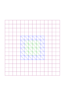
a) $\Omega=\Omega_{\rm FEM}\cup\Omega_{\rm FDM}$	b) $\Omega_{\rm FEM}=\Omega_{\rm IN}\cup\Omega_{\rm OUT}$	c) $\Omega_{\rm FDM}$

Figure 1:   Domain decomposition and mesh discretization in $\Omega$. The domain $\Omega$ presented on a) is a combination of the quadrilateral finite difference mesh $\Omega_{\rm FDM}$ presented on c), and the finite element mesh $\Omega_{\rm FEM}$ presented on b).

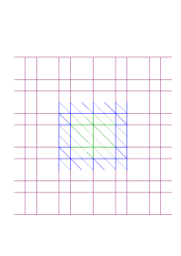
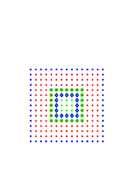
a) $\Omega=\Omega_{\rm FEM}\cup\Omega_{\rm FDM}$	b) $\Omega=\Omega_{\rm FEM}\cup\Omega_{\rm FDM}$

Figure 2:  Coupling between $\Omega_{\rm FEM}$ and $\Omega_{\rm FDM}$. The nodes of the FE/FD mesh of a) are presented also on b) as sets of following nodes: $\omega_{\rm o}$ (green circles), $\omega_{\diamond}$ (blue diamonds), $\omega_{*}$ (green stars), $\omega_{+}$ (red pluses), $\omega_{\rm x}$ (blue crosses). These sets are described in the domain decomposition algorithm.

We now describe the domain decomposition method between two domains $\Omega_{\rm FEM}$ and $\Omega_{\rm FDM}$ where FEM is used for computation of the solution in $\Omega_{\rm FEM}$, and FDM is used in $\Omega_{\rm FDM}$, see Figures 1, 2. Overlapping nodes between $\Omega_{\rm FDM}$ and $\Omega_{\rm FEM}$ are outlined in Figure 2 by green circles (boundary nodes of $\Omega_{\rm FEM}$) and blue diamonds (inner boundary nodes of $\Omega_{\rm FDM}$).

The communication between two domains $\Omega_{\rm FEM}$ and $\Omega_{\rm FDM}$ is achieved by overlapping of both meshes across a two-element thick layer around $\Omega_{\rm FEM}$ - see Figure 2. The nodes of the computational domain $\Omega$ belong to either of the following sets (see Figure 2-b)):

• Nodes ’$\rm o$’ - lie on the boundary $\partial\Omega_{\rm FEM}$ of $\Omega_{\rm FEM}$ and are interior to $\Omega_{\rm FDM}$,

• Nodes ’$\diamond$’ - lie on the inner boundary $\partial\Omega_{\rm FDM}$ of $\Omega_{\rm FDM}$ and are interior to $\Omega_{\rm FEM}$,

• Nodes ’$*$’ are interior to $\Omega_{\rm FEM}$,

• Nodes ’$+$’ are interior to $\Omega_{\rm FDM}$,

• Nodes ’$\rm x$’ lie on the outer boundary $\partial\Omega$ of $\Omega_{\rm FDM}$.

Then the main loop in time for the explicit schemes which solves the problem (6) with appropriate boundary conditions is shown in Algorithm 1.

Algorithm 1 The domain decomposition algorithm

1:  On the structured part of the mesh $\Omega_{\rm FDM}$, where FDM is used, update the Finite Difference (FD) solution at nodes $\omega_{+}$ and $\omega_{\diamond}$.

2:  On the unstructured part of the mesh $\Omega_{\rm FEM}$, where FEM is used, update the Finite Element (FE) solution at nodes $\omega_{*}$ and $\omega_{\rm o}$.

3:  Copy FE solution obtained at nodes $\omega_{\diamond}$ as a boundary condition for the FD solution in $\Omega_{\rm FDM}$.

4:  Copy FD solution obtained at nodes $\omega_{\rm o}$ as a boundary condition for the FE solution in $\Omega_{\rm FEM}$.

By conditions (2) functions $\varepsilon_{r}=1$ and $\sigma=0$ at the overlapping nodes between $\Omega_{\rm FEM}$ and $\Omega_{\rm FDM}$, and thus, the Maxwell’s equations will transform to the system of uncoupled acoustic wave equations (4) which leads to the fact that the FEM and FDM discretization schemes coincide on the common structured overlapping layer. In this way we avoid instabilities at interfaces in the domain decomposition algorithm.

4 Reconstruction algorithms

In this section we develop different optimization algorithms which allow determination of the relative dielectric permittivity function using scattered data of the electric field at the boundary of the investigated domain. In all algorithms we use assumption that the effective conductivity function is known in the investigated domain.

In summary, the main algorithms presented in this section are:

• Algorithm 2: The domain decomposition algorithm for efficient solution of forward and adjoint problems used in algorithms 3, 4, 5.

• Algorithm 3: Optimization algorithm for determination of the relative dielectric permittivity function under condition that the effective conductivity function is known.

• Algorithm 4, 5: Adaptive optimization algorithms for determination of the relative dielectric permittivity function. These algorithms use local adaptive mesh refinement based on a new error indicators for improved determination of location, material and sizes of the inclusions to be identified.

Let the domain decomposition of the computational domain $\Omega$ be as it is described in Section 3, see also Figures 2. We denote by $\Omega_{T}:=\Omega\times(0,T),\partial\Omega_{T}:=\partial\Omega\times(0,T),T>0$. Let the boundary $\partial\Omega=\partial\Omega_{\rm FDM}^{\rm out}\cup\partial\Omega_{\rm FDM}^{\rm in}$ be the outer boundary $\partial\Omega_{\rm FDM}^{\rm out}$ of $\Omega$ together with the inner boundary $\partial\Omega_{\rm FDM}^{\rm in}$ of $\Omega_{\rm FDM}$, and $\partial\Omega_{\rm FEM}$ be the boundary of $\Omega_{\rm FEM}$. Let at $S_{T}:=\partial\Omega_{\rm FDM}^{\rm out}\times(0,T)$ we have time-dependent backscattering observations.

Our coefficient inverse problem will be the following.

Inverse Problem (IP) Assume that the functions $\varepsilon_{r}(x),~{}\sigma(x)$  satisfy conditions (2) for known $d_{1}>1,$ $d_{2}>0$. Let the function $\varepsilon_{r}$ be unknown in the domain $\Omega\backslash(\Omega_{\rm FDM}\cup\Omega_{\rm OUT})$. Determine the function $\varepsilon_{r}(x)$ for $x\in\Omega\backslash(\Omega_{\rm FDM}\cup\Omega_{\rm OUT}),$  assuming that the function $\sigma(x)$ is known in $\Omega$ and the following function $\tilde{E}\left(x,t\right)$ is measured at $S_{T}$:

$$E\left(x,t\right)=\tilde{E}\left(x,t\right),\forall\left(x,t\right)\in S_{T}.$$ (7)

The function $\tilde{E}\left(x,t\right)$ in (7) represents the time-dependent measurements of all components of the electric wave field $E(x,t)=(E_{1},E_{2},E_{3})(x,t)$ at $S_{T}$.

To solve IP we minimize the corresponding Tikhonov functional and use a Lagrangian approach to do that. We present details of derivation of optimization algorithms in the next section.

4.1 Derivation of optimization algorithms

For solution of the IP for Maxwell’s system (6) it is natural to minimize the following Tikhonov functional

$$\begin{split}J(E,\varepsilon_{r})=\frac{1}{2}\int_{\Omega_{T}}(E-\tilde{E})^{2}z_{\delta}\delta_{\rm obs}~{}dsdt+\frac{1}{2}\gamma\int_{\Omega}(\varepsilon_{r}-\varepsilon^{0})^{2}~{}~{}dx,\end{split}$$ (8)

where $\tilde{E}$ is the observed electric field in (7) at the observation points located at $\partial\Omega_{\rm FDM}^{\rm out}$, $\delta_{\rm obs}=\sum\delta(\partial\Omega_{\rm FDM}^{\rm out})$ is a sum of delta-functions at the observations points located at $\partial\Omega_{\rm FDM}^{\rm out}$, $E$ satisfies the equations (6) and thus depends on $\varepsilon_{r},\sigma$. We denote by $\varepsilon^{0}$ the initial guess for $\varepsilon_{r}$, and by $\gamma$ the regularization parameter. Here, $z_{\delta}$ is a cut-off function ensuring the compatibility conditions for data, see details in [12].

Let us introduce the following spaces of real valued functions

$$\begin{split}H_{E}^{1}(\Omega_{T})&:=\{w\in H^{1}(\Omega_{T}):w(\cdot,0)=0\},\\ U^{1}&=((H_{E}^{1}(\Omega_{T})^{3}\times(H_{E}^{1}(\Omega_{T}))^{3}\times C\left(\overline{\Omega}\right),\\ U^{0}&=(L_{2}\left(\Omega_{T}\right))^{3}\times(L_{2}\left(\Omega_{T}\right))^{3}\times L_{2}\left(\Omega\right).\end{split}$$ (9)

To solve the minimization problem

$$\min_{\varepsilon_{r}}J(E,\varepsilon_{r})$$ (10)

we take into account conditions (2) on the function $\varepsilon_{r}$ and introduce the Lagrangian

$$\begin{split}L(u)&=J(E,\varepsilon_{r})\\ &+\int_{\Omega_{T}}\lambda\Big{(}\frac{1}{c^{2}}\varepsilon_{r}\frac{\partial^{2}E}{\partial t^{2}}-\nabla\cdot(\nabla E)-\nabla\nabla\cdot((\varepsilon_{r}\varepsilon_{0}-1)E)+\mu_{0}\sigma\frac{\partial E}{\partial t}\Big{)}~{}dxdt,\end{split}$$ (11)

where $u=(E,\lambda,\varepsilon_{r})$.

To solve the minimization problem (10) we find a stationary point of the Lagrangian with respect to $u$ satisfying $\forall\bar{u}=(\bar{E},\bar{\lambda},\bar{\varepsilon_{r}})$

$$L^{\prime}(u;\bar{u})=0,$$ (12)

where $L^{\prime}(u;\cdot)$ is the Jacobian of $L$ at $u$. For solution of the minimization problem (12) we develop conjugate gradient method for reconstruction of parameter $\varepsilon_{r}$.

To obtain optimality conditions from (12), we integrate by parts in space and time the Lagrangian (11), assuming that $\lambda(x,T)=\frac{\partial\lambda}{\partial t}\left(x,T\right)=0,\frac{\partial\lambda}{\partial t}=\frac{\partial\lambda}{\partial n}$, and impose such conditions on the function $\lambda$ that $L(E,\lambda,\varepsilon_{r}):=L(u)=J(E,\varepsilon_{r}).$ Using the facts that $\lambda(x,T)=\frac{\partial\lambda}{\partial t}(x,T)=0$, $\nabla\cdot(\varepsilon\lambda)=0$ and $\sigma=0,\varepsilon_{r}=1$ on $\partial\Omega$, together with initial and boundary conditions of (6), we get following optimality conditions for all $\bar{u}\in U^{1}$,

$$\begin{split}0&=\frac{\partial L}{\partial\lambda}(u)(\bar{\lambda})=-\int_{\Omega_{T}}\frac{1}{c^{2}}\varepsilon_{r}\frac{\partial\bar{\lambda}}{\partial t}\frac{\partial E}{\partial t}~{}dxdt+\int_{\Omega_{T}}(\nabla E)(\nabla\bar{\lambda})~{}dxdt\\ &+\varepsilon_{0}\int_{\Omega_{T}}(\nabla\cdot(\varepsilon_{r}E))(\nabla\cdot\bar{\lambda})~{}dxdt-\int_{\Omega_{T}}(\nabla\cdot E)(\nabla\cdot\bar{\lambda})~{}dxdt\\ &+\int_{\Omega_{T}}\mu_{0}\sigma\frac{\partial E}{\partial t}\bar{\lambda}~{}dxdt-\int_{\Omega}\frac{\varepsilon_{r}}{c^{2}}\bar{\lambda}(x,0)f_{1}(x)~{}dx\\ &+\int_{\partial\Omega_{T}}\bar{\lambda}\frac{\partial E}{\partial t}~{}d\sigma dt,~{}~{}\forall\bar{\lambda}\in H_{\lambda}^{1}(\Omega_{T});\end{split}$$ (13)

$$\begin{split}0&=\frac{\partial L}{\partial E}(u)(\bar{E})=\int_{\Omega_{T}}(E-\widetilde{E})~{}\bar{E}~{}z_{\delta}\delta_{\rm obs}~{}d\sigma dt-\int_{\Omega}\frac{\varepsilon_{r}}{c^{2}}\frac{\partial{\lambda}}{\partial t}(x,0)\bar{E}(x,0)~{}dx\\ &-\int_{\partial\Omega_{T}}\frac{\partial{\lambda}}{\partial t}\bar{E}~{}d\sigma dt-\int_{\Omega_{T}}\frac{\varepsilon_{r}}{c^{2}}\frac{\partial\lambda}{\partial t}\frac{\partial\bar{E}}{\partial t}~{}dxdt+\int_{\Omega_{T}}(\nabla\lambda)(\nabla\bar{E})~{}dxdt\\ &+\varepsilon_{0}\int_{\Omega_{T}}(\nabla\cdot(\varepsilon_{r}\bar{E}))(\nabla\cdot\lambda)~{}dxdt-\int_{\Omega_{T}}(\nabla\cdot\bar{E})(\nabla\cdot\lambda)~{}dxdt\\ &-\int_{\Omega_{T}}\mu_{0}\sigma\bar{E}\frac{\partial\lambda}{\partial t}~{}dxdt,~{}\forall\bar{E}\in H_{E}^{1}(\Omega_{T}).\end{split}$$ (14)

Finally, we obtain the main equation for iterative update $\varepsilon_{r}$ in the conjugate gradient algorithm which express that the gradient with respect to $\varepsilon_{r}$ vanishes:

$$\begin{split}0&=\frac{\partial L}{\partial\varepsilon_{r}}(u)(\bar{\varepsilon}_{r})=-\int_{\Omega}\frac{\bar{\varepsilon}_{r}}{c^{2}}\lambda(x,0)f_{1}(x)~{}dx-\int_{\Omega_{T}}\frac{\bar{\varepsilon}_{r}}{c^{2}}\frac{\partial\lambda}{\partial t}\frac{\partial E}{\partial t}~{}dxdt\\ &+\varepsilon_{0}\int_{\Omega_{T}}(\nabla\cdot\lambda)(\nabla\cdot(\bar{\varepsilon}_{r}E))~{}dxdt+\gamma\int_{\Omega}(\varepsilon_{r}-\varepsilon^{0})\bar{\varepsilon}_{r}~{}dx,~{}x\in\Omega.\end{split}$$ (15)

The equation (13) is the weak formulation of the forward problem (6) and the equation (14) is the weak formulation of the following adjoint problem

$$\begin{array}[]{ll}\frac{1}{c^{2}}\varepsilon_{r}\frac{\partial^{2}\lambda}{\partial t^{2}}-\triangle\lambda-\varepsilon_{0}\varepsilon_{r}\nabla(\nabla\cdot\lambda)+\nabla(\nabla\cdot\lambda)-\mu_{0}\sigma\frac{\partial\lambda}{\partial t}=-(E-\widetilde{E})z_{\delta}\delta_{\rm obs}&\mbox{ in }\Omega_{T},\\ \lambda(\cdot,T)=\frac{\partial\lambda}{\partial t}(\cdot,T)=0&\mbox{ in }\Omega,\\ \frac{\partial\lambda}{\partial n}=\frac{\partial\lambda}{\partial t}&\mbox{ on }S_{T}.\end{array}$$ (16)

4.2 The domain decomposition FE/FD method for solution of forward and adjoint problems

4.2.1 Finite element discretization

We denote by $\Omega_{\rm FEM_{T}}:=\Omega_{\rm FEM}\times(0,T),\partial\Omega_{\rm FEM_{T}}:=\partial\Omega_{\rm FEM}\times(0,T),T>0$ where $\partial\Omega_{\rm FEM}$ is the boundary of $\Omega_{\rm FEM}$, and discretize $\Omega_{{\rm FEM}_{T}}$ denoting by $K_{h}=\{K\}$ a partition of the domain $\Omega_{\rm FEM}$ into elements $K$ such that

$$K_{h}=\cup_{K\in K_{h}}K=K_{1}\cup K_{2}...\cup K_{l},$$

where $l$ is the total number of elements $K$ in $\overline{\Omega}_{\rm FEM}$.

Here, $h=h(x)$ is a piecewise-constant mesh function defined as

$$h|_{K}=h_{K}~{}~{}~{}\forall K\in K_{h},$$ (17)

representing the local diameter of the elements. We also denote by $\partial K_{h}=\{\partial K\}$ a partition of the boundary $\partial\Omega_{\rm FEM}$ into boundaries $\partial K$ of the elements $K$ such that vertices of these elements belong to $\partial\Omega_{\rm FEM}$. We let $J_{\tau}$ be a partition of the time interval $(0,T)$ into time intervals $J=(t_{k-1},t_{k}]$ of uniform length $\tau=T/N$ for a given number of time steps $N$. We assume also a minimal angle condition on the $K_{h}$ [11, 35].

To formulate the finite element method in $\Omega$ for (12) we define the finite element spaces $C_{h}$, $W_{h}^{E}$. First, we introduce the finite element trial space $W_{h}^{E}$ for every component of the electric field $E$ defined by

$$W_{h}^{E}:=\{w\in H_{E}^{1}:w|_{K}\in P_{1}(K),\forall K\in K_{h}\},$$

where $P_{1}(K)$ denote the set of piecewise-linear functions on $K$.

To approximate function $\varepsilon_{r}$ we define the space of piecewise constant functions $C_{h}\subset L_{2}(\Omega)$,

$$C_{h}:=\{u\in L_{2}(\Omega):u|_{K}\in P_{0}(K),\forall K\in K_{h}\},$$ (18)

where $P_{0}(K)$ is the piecewise constant function on $K$. Setting ${\textbf{W}_{h}^{E}(\Omega)}:=[W_{h}^{E}(\Omega)]^{3}$ we define $U_{h}={\textbf{W}_{h}^{E}(\Omega)}\times{\textbf{W}_{h}^{E}(\Omega)}\times C_{h}$. The finite element method for (12) now reads: find $u_{h}:U_{h}\times[0,T]\to\mathbb{R}$, such that

$$L^{\prime}(u_{h})(\bar{u})=0,~{}\forall\bar{u}\in U_{h}.$$ (19)

The equation (19) expresses discretized versions of optimality conditions given by (13)-(15). To get function $\varepsilon_{r}$ via optimality condition (15) we need solutions first of the forward problem (6), and then of the adjoint problem (16). To solve these problems via the domain decomposition method, we decompose the computational domain $\Omega=\Omega_{\rm FEM}\cup\Omega_{\rm FDM}$ as it is described in section 3. Thus, in $\Omega_{\rm FEM}$ we have to solve the following forward problem:

$$\begin{array}[]{ll}\frac{1}{c^{2}}\varepsilon_{r}\frac{\partial^{2}E}{\partial t^{2}}+\nabla(\nabla\cdot E)-\triangle E-\varepsilon_{0}\nabla(\nabla\cdot(\varepsilon_{r}E))=-\mu_{0}\sigma\frac{\partial E}{\partial t}&\mbox{ in }\Omega_{\rm FEM}\times(0,T),\\ E(\cdot,0)=f_{0},\mbox{ and }\frac{\partial E}{\partial t}(\cdot,0)=f_{1}&\mbox{ in }\Omega_{\rm FEM},\\ \frac{\partial E}{\partial n}=g&\mbox{ on }\partial\Omega_{\rm FEM}\times(0,T).\end{array}$$ (20)

Here, $g$ is the solution obtained by the finite difference method in $\Omega_{\rm FDM}$ which is saved at $\partial\Omega_{\rm FEM}$.

The equation (19) expresses that the finite element method in $\Omega_{\rm FEM}$ for the solution of the forward problem (20) will be: Find $E_{h}:{\textbf{W}_{h}^{E}(\Omega_{\rm FEM})}\times[0,T]\to\mathbb{R}$, such that $\forall\bar{\lambda}\in{\textbf{W}_{h}^{E}(\Omega_{\rm FEM})}$

$$\begin{array}[]{l}\frac{1}{c^{2}}\left({\varepsilon_{r}}_{h}\frac{\partial^{2}E_{h}}{\partial t^{2}},\bar{\lambda}\right)+(\nabla E_{h},\nabla\bar{\lambda})+\varepsilon_{0}(\nabla\cdot({\varepsilon_{r}}_{h}E_{h}),\nabla\cdot\bar{\lambda})-(\nabla\cdot E_{h},\nabla\cdot\bar{\lambda})\\ +(g_{h},\bar{\lambda})_{\partial\Omega_{\rm FEM}}+\mu_{0}(\sigma_{h}\frac{\partial E_{h}}{\partial t},\bar{\lambda})=0,\\ E_{h}(\cdot,0)={f_{0}}_{h}\mbox{ and }\frac{\partial E_{h}}{\partial t}(\cdot,0)={f_{1}}_{h}\mbox{ in }\Omega_{\rm FEM}.\end{array}$$ (21)

Here, we define ${f_{0}}_{h},{f_{1}}_{h},g_{h},{\varepsilon_{r}}_{h},\sigma_{h}$ to be the usual ${\textbf{W}_{h}^{E}}$-interpolate of $f_{0},f_{1},g,\varepsilon_{r},\sigma$ in (6) in $\Omega_{\rm FEM}$.

To get the discrete scheme for (21) we approximate $E_{h}(k\tau)$ by $E_{h}^{k}$ for $k=1,2,...,N$ using the following scheme for $k=1,2,\ldots,N-1$ and $\forall\bar{\lambda}\in{\textbf{W}_{h}^{E}(\Omega_{\rm FEM})}$

$$\begin{array}[]{l}\frac{1}{c^{2}}\left({\varepsilon_{r}}_{h}\frac{E_{h}^{k+1}-2E_{h}^{k}+E_{h}^{k-1}}{\tau^{2}},\bar{\lambda}\right)+(\nabla E_{h}^{k},\nabla\bar{\lambda})+\varepsilon_{0}(\nabla\cdot({\varepsilon_{r}}_{h}E_{h}^{k}),\nabla\cdot\bar{\lambda})-(\nabla\cdot E_{h}^{k},\nabla\cdot\bar{\lambda})\\ +(g_{h}^{k},\bar{\lambda})_{\partial\Omega_{\rm FEM}}+\mu_{0}(\sigma_{h}\frac{E_{h}^{k+1}-E_{h}^{k-1}}{2\tau},\bar{\lambda})=0,\\ {E_{h}}^{0}={f_{0}}_{h}\mbox{ and }{E_{h}}^{1}={E_{h}}^{0}+\tau{f_{1}}_{h}\mbox{ in }\Omega_{\rm FEM}.\end{array}$$ (22)

Rearranging terms in (22) we get for $k=1,2,\ldots,N-1$ and $\forall\bar{\lambda}\in{\textbf{W}_{h}^{E}(\Omega_{\rm FEM})}$

$$\begin{split}&\left((1+\tau c^{2}\mu_{0}\frac{\sigma_{h}}{2{\varepsilon_{r}}_{h}})E_{h}^{k+1},\bar{\lambda}\right)=\left(2E_{h}^{k},\bar{\lambda}\right)-\left(E_{h}^{k-1},\bar{\lambda}\right)-\tau^{2}c^{2}(1/{\varepsilon_{r}}_{h}\nabla E_{h}^{k},\nabla\bar{\lambda})\\ &-\tau^{2}c^{2}\varepsilon_{0}(1/{\varepsilon_{r}}_{h}\nabla\cdot({\varepsilon_{r}}_{h}E_{h}^{k}),\nabla\cdot\bar{\lambda})+\tau^{2}c^{2}(1/{\varepsilon_{r}}_{h}\nabla\cdot E_{h}^{k},\nabla\cdot\bar{\lambda})\\ &+\tau^{2}c^{2}\left(\frac{g_{h}^{k}}{{\varepsilon_{r}}_{h}},\bar{\lambda}\right)_{\partial\Omega_{\rm FEM}}+\tau c^{2}\mu_{0}(\frac{\sigma_{h}}{2{\varepsilon_{r}}_{h}}E_{h}^{k-1},\bar{\lambda}),\\ &E_{h}^{0}={f_{0}}_{h}\mbox{ and }E_{h}^{1}=E_{h}^{0}+\tau{f_{1}}_{h}\mbox{ in }\Omega_{\rm FEM}.\end{split}$$ (23)

The adjoint problem in $\Omega_{\rm FEM}$ will be the following:

$$\begin{split}&\frac{1}{c^{2}}\varepsilon_{r}\frac{\partial^{2}\lambda}{\partial t^{2}}-\triangle\lambda-\varepsilon_{0}\varepsilon_{r}\nabla(\nabla\cdot\lambda)+\nabla(\nabla\cdot\lambda)-\mu_{0}\sigma\frac{\partial\lambda}{\partial t}=-(E-\widetilde{E})z_{\delta}\delta_{\rm obs}\mbox{ in }\Omega_{\rm FEM}\times(0,T),\\ &\lambda(\cdot,T)=\frac{\partial\lambda}{\partial t}(\cdot,T)=0\mbox{~{} ~{}~{} for~{}~{}~{}~{} }x\in\Omega_{\rm FEM},\\ &\frac{\partial\lambda}{\partial n}=p~{}\mbox{~{}~{}~{}on~{}~{}~{}}~{}\partial\Omega_{\rm FEM_{T}}.\end{split}$$ (24)

The finite element method for the solution of adjoint problem (24) in $\Omega_{\rm FEM}$ reads: Find $\lambda_{h}\in{\textbf{W}_{h}^{E}(\Omega_{\rm FEM})}$ such that $\forall\bar{E}\in{\textbf{W}_{h}^{E}(\Omega_{\rm FEM})}$

$$\begin{array}[]{l}\frac{1}{c^{2}}\left({\varepsilon_{r}}_{h}\frac{\partial^{2}\lambda_{h}}{\partial t^{2}},\bar{E}\right)+(\nabla\lambda_{h},\nabla\bar{E})+\varepsilon_{0}(\nabla\cdot\lambda_{h},\nabla\cdot({\varepsilon_{r}}_{h}\bar{E}))-(\nabla\cdot\lambda_{h},\nabla\cdot\bar{E})\\ -(p_{h},\bar{E})_{\partial\Omega_{\rm FEM}}-\mu_{0}(\sigma_{h}\frac{\lambda_{h}}{t},\bar{\lambda})=-((E_{h}-\widetilde{E}_{h})z_{\delta}\delta_{\rm obs},\bar{E}).\end{array}$$ (25)

Here, we define $E_{h},\widetilde{E}_{h},p_{h}$ to be the usual ${\textbf{W}_{h}^{E}}$-interpolate of $E,\widetilde{E},p$ in (24) in $\Omega_{\rm FEM}$.

We note that the adjoint problem should be solved backwards in time, from time $t=T$ to $t=0$. To get the discrete scheme for (25) we approximate $\lambda_{h}(k\tau)$ by $\lambda_{h}^{k}$ for $k=N,N-1,...,1$ using the following scheme for $k=N-1,\ldots,1$:

$$\begin{array}[]{l}\frac{1}{c^{2}}\left({\varepsilon_{r}}_{h}\frac{\lambda_{h}^{k+1}-2\lambda_{h}^{k}+\lambda_{h}^{k-1}}{\tau^{2}},\bar{E}\right)+(\nabla\lambda_{h}^{k},\nabla\bar{E})+\varepsilon_{0}(\nabla\cdot\lambda_{h}^{k},\nabla\cdot({\varepsilon_{r}}_{h}\bar{E}))-(\nabla\cdot\lambda_{h}^{k},\nabla\cdot\bar{E})\\ -\left(p_{h}^{k},\bar{E}\right)_{\partial\Omega_{\rm FEM}}-\mu_{0}(\sigma_{h}\frac{\lambda_{h}^{k+1}-\lambda_{h}^{k-1}}{2\tau},\bar{E})=-((E_{h}^{k}-\widetilde{E}_{h}^{k})z_{\delta}\delta_{\rm obs},\bar{E})\;\forall\bar{\lambda}\in{\textbf{W}_{h}^{E}(\Omega_{\rm FEM})}.\end{array}$$ (26)

Multiplying both sides of (26) by $\tau^{2}c^{2}/{\varepsilon_{r}}_{h}$ and rearranging the terms we obtain:

$$\begin{split}&\left((1+\tau c^{2}\mu_{0}\frac{\sigma_{h}}{2{\varepsilon_{r}}_{h}})\lambda_{h}^{k-1},\bar{E}\right)=\left(2\lambda_{h}^{k},\bar{E}\right)-\left(\lambda_{h}^{k+1},\bar{E}\right)-\tau^{2}c^{2}(1/{\varepsilon_{r}}_{h}\nabla\lambda_{h}^{k},\nabla\bar{E})\\ &-\tau^{2}c^{2}\varepsilon_{0}(1/{\varepsilon_{r}}_{h}\nabla\cdot\lambda_{h}^{k},\nabla\cdot({\varepsilon_{r}}_{h}\bar{E}))+\tau^{2}c^{2}(1/{\varepsilon_{r}}_{h}\nabla\cdot\lambda_{h}^{k},\nabla\cdot\bar{E})\\ &+\tau^{2}c^{2}\left(\frac{p_{h}^{k}}{{\varepsilon_{r}}_{h}},\bar{E}\right)_{\partial\Omega_{\rm FEM}}+\tau c^{2}\mu_{0}(\frac{\sigma_{h}}{2{\varepsilon_{r}}_{h}}\lambda_{h}^{k+1},\bar{E})-\tau^{2}c^{2}(1/{\varepsilon_{r}}_{h}(E_{h}^{k}-\widetilde{E}_{h}^{k})z_{\delta}\delta_{\rm obs},\bar{E}),\end{split}$$ (27)

for $k=N-1,\ldots,1$, $\forall\bar{E}\in{\textbf{W}_{h}^{E}(\Omega_{\rm FEM})}$

We note that usually $\dim U_{h}<\infty$ and $U_{h}\subset U^{1}$ as a set and we consider $U_{h}$ as a discrete analogue of the space $U^{1}.$ We introduce the same norm in $U_{h}$ as the one in $U^{0}$,

$$\left\|\bullet\right\|_{U_{h}}:=\left\|\bullet\right\|_{U^{0}},$$ (28)

where $U_{0}$ is defined in (9). From (28) follows that all norms in finite dimensional spaces are equivalent. This allows us in numerical simulations of section 5 compute the discrete function ${\varepsilon_{r}}_{h}$, which is approximation of $\varepsilon_{r}(x)$, in the space $C_{h}$.

4.3 Fully discrete scheme in $\Omega_{\rm FEM}$

In this section we present schemes for computations of the solutions of forward (6) and adjoint (16) problems in $\Omega_{\rm FEM}$. After expanding functions $E_{h}(x)$ and $\lambda_{h}(x)$ in terms of the standard continuous piecewise linear functions $\{\varphi_{i}(x)\}_{i=1}^{M}$ in space as

$$\begin{split}E_{h}(x)=\sum_{i=1}^{M}E_{h_{i}}\varphi_{i}(x),~{}\lambda_{h}(x)&=\sum_{i=1}^{M}\lambda_{h_{i}}\varphi_{i}(x),\end{split}$$

where $E_{h_{i}}$ and $\lambda_{h_{i}}$ denote unknown coefficients at the mesh point $x_{i}\in K_{h},i=1,...,M$, substitute them into (23) and (27), correspondingly, with $\bar{\lambda}(x,t)=\bar{E}(x,t)=\sum_{j=1}^{M}\varphi_{j}(x)$, and obtain the system of linear equations for computation of the forward problem (6):

$$\begin{split}M_{1}E^{k+1}&=2ME^{k}-ME^{k-1}-\tau^{2}c^{2}G_{1}E^{k}-\tau^{2}c^{2}\varepsilon_{0}G_{2}E^{k}\\ &+\tau^{2}c^{2}G_{3}E^{k}+\tau^{2}c^{2}F^{k}+\tau c^{2}\mu_{0}M_{2}E^{k-1}.\end{split}$$ (29)

Here, $M,M_{1},M_{2}$ are the assembled block mass matrices in space, $G_{1},G_{2},G_{3}$ are the assembled block matrices in space, $F^{k}$ is the assembled load vector at the time iteration $k$, $E^{k}$ denote the nodal values of $E_{h}(\cdot,t_{k})$, $\tau$ is the time step. Now we define the mapping $F_{K}$ for the reference element $\hat{K}$ such that $F_{K}(\hat{K})=K$ and let $\hat{\varphi}$ be the piecewise linear local basis function on the reference element $\hat{K}$ such that $\varphi\circ F_{K}=\hat{\varphi}$. Then, the explicit formulas for the entries in system of equations (29) at each element $K$ can be given as:

$$\begin{split}M_{{i,j}}^{K}&=(\varphi_{i}(x)\circ F_{K},\varphi_{j}(x)\circ F_{K})_{K},\\ {M_{1}}_{{i,j}}^{K}&=((1+\tau c^{2}\mu_{0}\frac{\sigma_{h}}{2\varepsilon_{r_{h}}})\varphi_{i}(x)\circ F_{K},\varphi_{j}(x)\circ F_{K})_{K},\\ {M_{2}}_{{i,j}}^{K}&=(\frac{\sigma_{h}}{2{\varepsilon_{r}}_{h}}\varphi_{i}(x)\circ F_{K},\varphi_{j}(x)\circ F_{K})_{K},\\ {G_{1}}_{{i,j}}^{K}&=(\frac{1}{{\varepsilon_{r}}_{h}}\nabla\varphi_{i}\circ F_{K},\nabla\varphi_{j}\circ F_{K})_{K},\\ {G_{2}}_{{i,j}}^{K}&=(\frac{1}{{\varepsilon_{r}}_{h}}\nabla\cdot({\varepsilon_{r}}_{h}\varphi_{i})\circ F_{K},\nabla\cdot\varphi_{j}\circ F_{K})_{K},\\ {G_{3}}_{{i,j}}^{K}&=(\frac{1}{\varepsilon_{r_{h}}}\nabla\cdot\varphi_{i}\circ F_{K},\nabla\cdot\varphi_{j}\circ F_{K})_{K},\\ F_{j}^{k}&=(\frac{g_{h}^{k}}{\varepsilon_{r_{h}}},\varphi_{j}\circ F_{K})_{\partial K},\end{split}$$ (30)

where $(\cdot,\cdot)_{K}$ denotes the $L_{2}(K)$ scalar product and $\partial K$ is the part of the boundary of element $K$ which lies at $\partial\Omega_{\rm FEM}$.

For the case of adjoint problem (27) we get the system of linear equations:

$$\begin{split}M_{1}\lambda^{k-1}&=2M\lambda^{k}-M\lambda^{k+1}-\tau^{2}c^{2}G_{1}\lambda^{k}-\tau^{2}c^{2}\varepsilon_{0}G_{2}^{T}\lambda^{k}\\ &+\tau^{2}c^{2}G_{3}\lambda^{k}+\tau^{2}c^{2}P_{1}^{k}+\tau c^{2}\mu_{0}M_{2}\lambda^{k+1}-\tau^{2}c^{2}P_{2}^{k}.\end{split}$$ (31)

Here, $M,M_{1},M_{2},G_{1},G_{2},G_{3}$ are the assembled block matrices in space with explicit entries given in (30), and $P_{1}^{k},P_{2}^{k}$ are assembled load vectors at the time iteration $k$ with explicit entries

$$\begin{split}{P_{1}}_{j}^{k}&=(\frac{p_{h}^{k}}{{\varepsilon_{r}}_{h}},\varphi_{j}\circ F_{K})_{\partial K},\\ {P_{2}}_{j}^{k}&=(1/{\varepsilon_{r}}_{h}(E_{h}^{k}-\widetilde{E}_{h}^{k})z_{\delta}\delta_{\rm obs},\varphi_{j}\circ F_{K})_{K},\end{split}$$ (32)

$\lambda^{k}$ denote the nodal values of $\lambda_{h}(\cdot,t_{k})$, $\tau$ is the time step.

Finally, for reconstructing $\varepsilon_{r}(x)$ in $\Omega_{IN}$ we can use a gradient-based method with an appropriate initial guess values $\varepsilon^{0}$. The discrete versions in space of the gradients given in (15), after integrating by parts in space of the third term in the right hand side of (15), have the form $\forall x\in\Omega_{\rm IN}$:

$$\begin{split}{g_{h}}&=-\frac{1}{c^{2}}\lambda_{h}(x,0){f_{1}}_{h}-\frac{1}{c^{2}}\int_{0}^{T}\frac{\partial\lambda_{h}}{\partial t}\frac{\partial E_{h}}{\partial t}~{}dt\\ &+\varepsilon_{0}\int_{0}^{T}(\nabla\cdot\lambda_{h})(\nabla\cdot E_{h})~{}dt+\gamma({\varepsilon_{r}}_{h}-\varepsilon_{h}^{0}),\end{split}$$ (33)

where $\varepsilon_{h}^{0}$ is interpolant of $\varepsilon^{0}$. We note that because of usage of the domain decomposition method, gradient (33) should be updated only in $\Omega_{IN}$ since in $\Omega_{\rm FDM}$ and in $\Omega_{\rm OUT}$ by condition (2) we have $\varepsilon_{r}=1,\sigma=0$. In (33) $E_{h}$ and $\lambda_{h}$ are computed values of the forward and adjoint problems using schemes (29), (31), correspondingly, and ${\varepsilon_{r}}_{h}$ is approximate value of the computed relative dielectric permittivity function $\varepsilon_{r}$.

4.3.1 Finite difference formulation

We recall now that from conditions (2) it follows that in $\Omega_{\rm FDM}$ the function $\varepsilon_{r}(x)=1,\sigma=0$. This means that in $\Omega_{\rm FDM}$ the model problem (6) transforms to the following forward problem for uncoupled system of acoustic wave equations for $E=(E_{1},E_{2},E_{3})$:

$$\frac{\partial^{2}E}{\partial t^{2}}-\Delta E=0 ~{}~{}\mbox{in}~{}~{}\Omega_{\rm FDM}\times(0,T),$$

$$E(\cdot,0)=f_{0},~{}~{}~{}\frac{\partial E}{\partial t}(\cdot,0)=f_{1} ~{}~{}\mbox{in}~{}~{}\Omega_{\rm FDM},$$

$$\frac{\partial E}{\partial n}=-\frac{\partial E}{\partial t} ~{}~{}\mbox{on}~{}S_{T},$$

$$\frac{\partial E}{\partial n}=\frac{\partial E_{\rm FEM}}{\partial n} ~{}~{}\mbox{on}~{}\partial\Omega_{\rm FDM}^{\rm in},$$

where $\frac{\partial E_{\rm FEM}}{\partial n}$ are known values at $\partial\Omega_{\rm FDM}^{\rm in}$.

Using standard finite difference discretization of the first equation in  (4.3.1) in $\Omega_{\rm FDM}$ we obtain the following explicit scheme for every component of the solution $E$ of the forward problem (4.3.1)

$$E_{l,j,m}^{k+1}=\tau^{2}\Delta E_{l,j,m}^{k}+2E_{l,j,m}^{k}-E_{l,j,m}^{k-1},$$ (34)

with correspondingly discretized absorbing boundary conditions. In equations above, $E_{l,j,m}^{k}$ is the finite difference solution on the time iteration $k$ at the discrete point $(l,j,m)$, $\tau$ is the time step, and $\Delta E_{l,j,m}^{k}$ is the discrete Laplacian.

The adjoint problem in $\Omega_{\rm FDM}$ will be:

$$\begin{split}\frac{\partial^{2}\lambda}{\partial t^{2}}-\Delta\lambda=-(E-\widetilde{E})z_{\delta}\delta_{\rm obs}&~{}~{}\mbox{in}~{}~{}\Omega_{\rm FDM}\times(0,T),\\ \lambda(\cdot,T)=\frac{\partial\lambda}{\partial t}(\cdot,T)=0&~{}~{}\mbox{in}~{}~{}\Omega_{\rm FDM},\\ \frac{\partial\lambda}{\partial n}=\frac{\partial\lambda}{\partial t}&~{}~{}\mbox{on}~{}~{}S_{T},\\ \frac{\partial\lambda}{\partial n}=\frac{\partial\lambda_{\rm FEM}}{\partial n}&~{}~{}\mbox{on}~{}~{}\partial\Omega_{\rm FDM}^{\rm in},\\ \end{split}$$ (35)

where $\frac{\partial\lambda_{\rm FEM}}{\partial n}$ are known values at $\partial\Omega_{\rm FDM}^{\rm in}$.

Similarly with (36) we get the following explicit scheme for the solution of adjoint problem (35) in $\Omega_{FDM}$ which we solve backward in time:

$$\lambda_{l,j,m}^{k-1}=-\tau^{2}(E-\widetilde{E})_{l,j,m}^{k}z_{\delta}\delta_{\rm obs}+\tau^{2}\Delta\lambda_{l,j,m}^{k}+2\lambda_{l,j,m}^{k}-\lambda_{l,j,m}^{k+1},$$ (36)

with corresponding boundary conditions. In equations (34), (36) $(\cdot)_{l,j,m}^{k}$ is the solution on the time iteration $k$ at the discrete point $(l,j,m)$,

We note that we use FDM only inside $\Omega_{\rm FDM}$, and thus computed values of $\frac{\partial E_{\rm FEM}}{\partial n}$ and $\frac{\partial\lambda_{\rm FEM}}{\partial n}$ can be approximated and will be known at $\partial\Omega_{\rm FDM}^{\rm in}$ through the finite element solution in $\Omega_{\rm FEM}$, see details in the domain decomposition Algorithm 2.

4.4 The domain decomposition algorithm to solve forward and adjoint problems

First we present domain decomposition algorithm for the solution of state and adjoint problems. We note that because of using explicit finite difference scheme in $\Omega_{\rm FDM}$ we need to choose time step $\tau$ accordingly to the CFL stability condition [5, 6, 15] such that the whole scheme remains stable.

Algorithm 2 The domain decomposition algorithm to solve forward and adjoint problems

1:  Construct the finite element mesh $K_{h}$ in $\Omega_{\rm FEM}$ and the finite difference mesh in $\Omega_{\rm FDM}$ as well as time partition $J_{\tau}$ of the time interval $\left(0,T\right)$. At every time step $k$ we perform the following operations:

2:  On the mesh in $\Omega_{\rm FDM}$ compute $E^{k+1}$, $\lambda^{k-1}$ from (34), (36), correspondingly, using absorbing boundary conditions at the outer boundary $\partial\Omega$, with $E^{k},E^{k-1}$ and $\lambda^{k},\lambda^{k+1}$ known.

3:  On the mesh $K_{h}$ in $\Omega_{\rm FEM}$ compute $E^{k+1},\lambda^{k-1}$ using the finite element schemes (29), (31), correspondingly, with $E^{k},E^{k-1}$ and $\lambda^{k},\lambda^{k+1}$ known.

4:  Use the values of the functions $E^{k+1},\lambda^{k-1}$ at nodes $\omega_{*}$ overlapping with nodes $\omega_{\diamond}$, which are computed using the finite element schemes (29), (31), correspondingly, as a boundary conditions at the inner boundary $\partial\Omega_{\rm FDM}^{\rm in}$ for the finite difference method in $\Omega_{\rm FDM}$.

5:  Use the values of the functions $E^{k+1},\lambda^{k-1}$ at nodes $\omega_{\rm o}$ overlapping with nodes $\omega_{\rm+}$, which are computed using the finite difference schemes (34), (36), correspondingly, as a boundary conditions at $\partial\Omega_{\rm FEM}$ for the finite element method in $\Omega_{\rm FEM}$.

6:  Apply swap of the solutions for the computed functions $E^{k+1},\lambda^{k-1}$. Set $k=k+1$ for forward problem and $k=k-1$ for adjoint problem and go to step 2.

4.5 Reconstruction algorithm for the solution of inverse problem IP

We use conjugate gradient method (CGM) for iterative update of approximation ${\varepsilon_{r}}_{h}^{m}$ of the function ${\varepsilon_{r}}_{h}$, where $m$ is the number of iteration in the optimization algorithm. We introduce the following function

$$\begin{split}{g}_{h}^{m}(x)&=-\frac{1}{c^{2}}\lambda_{h}^{m}(x,0){f_{1}}_{h}(x)-\frac{1}{c^{2}}\int_{0}^{T}\frac{\partial\lambda_{h}^{m}}{\partial t}\frac{\partial E_{h}^{m}}{\partial t}~{}dt\\ &+\varepsilon_{0}\int_{0}^{T}(\nabla\cdot\lambda_{h}^{m})(\nabla\cdot E_{h}^{m})~{}dt+\gamma({\varepsilon_{r}}_{h}^{m}-\varepsilon_{h}^{0}),\end{split}$$ (37)

where functions $E_{h}^{m},\lambda_{h}^{m}$ are computed by solving the state and adjoint problems with $\varepsilon_{r}:={\varepsilon_{r}}_{h}^{m},\sigma:=\sigma_{h}^{m}$.

Algorithm 3 Conjugate gradient algorithm for determination of the relative dielectric permittivity function

1:  Initialize the mesh in $\Omega$ and time partition $J_{\tau}$ of the time interval $\left(0,T\right).$ Start with the initial approximation ${\varepsilon_{r}}_{h}^{0}=\varepsilon_{h}^{0}$ with known ${\sigma}_{h}$, and compute the sequence of ${\varepsilon_{r}}_{h}^{m}$ via the following steps:

2:  Compute solutions $E_{h}(x,t,{\varepsilon_{r}}_{h}^{m},\sigma_{h})$ and $\lambda_{h}\left(x,t,{\varepsilon_{r}}_{h}^{m},\sigma_{h}\right)$ of forward and adjoint problems on $K_{h}$ and $J_{\tau}$ using the domain decomposition algorithm (Algorithm 2).

3:  Update the function ${\varepsilon_{r}}_{h}:={\varepsilon_{r}}_{h}^{m+1}$ on $K_{h}$ and $J_{\tau}$ using the CGM as

$$\begin{split}{\varepsilon_{r}}_{h}^{m+1}&={\varepsilon_{r}}_{h}^{m}+\alpha d^{m}(x),\\ \end{split}$$

where $\alpha$ is the step-size in the gradient update [48] and

$$\begin{split}d^{m}(x)&=-g_{h}^{m}(x)+\beta^{m}d^{m-1}(x),\\ \end{split}$$

with

$$\begin{split}\beta^{m}&=\frac{\|g_{h}^{m}(x)\|^{2}}{\|g_{h}^{m-1}(x)\|^{2}},\\ \end{split}$$

Here, $d^{0}(x)=-g_{h}^{0}(x)$.

4:  Stop computing ${\varepsilon_{r}}_{h}^{m}$ at the iteration $M:=m$ and obtain the function ${\varepsilon_{r}}_{h}^{M}:={\varepsilon_{h}}_{r}^{m}$ if either $\|g_{h}^{m}\|_{L_{2}(\Omega)}\leq\theta$ or norms $\|{\varepsilon_{r}}_{h}^{m}\|_{L_{2}(\Omega)}$ are stabilized. Here, $\theta$ is the tolerance chosen by the user. Otherwise set $m:=m+1$ and go to step 2.

4.6 Adaptive algorithms for solution of the inverse problem IP

Adaptive algorithm allows improvement of already computed relative dielectric permittivity function ${\varepsilon_{r}}_{h}^{M}$ obtained on the initially non-refined mesh in the previous optimization algorithm (Algorithm 3). The idea of the local mesh refinement (note that we need it only in $\Omega_{IN}$) is that it should be refined in all neighborhoods of all points in the mesh $K_{h}$ where the function $|h{\varepsilon_{r}}_{h}|$ achieves its maximum value, or where $|J_{\varepsilon_{r}}^{\prime}({\varepsilon_{r}}_{h})|$ achieves its maximal values. These local mesh refinements recommendations are based on a posteriori error estimates for the error $|\varepsilon_{r}-{\varepsilon_{r}}_{h}|$ in the reconstructed function $\varepsilon_{r}$ ( see the first mesh refinement indicator), and for the error $|J({\varepsilon_{r}})-J({\varepsilon_{r}}_{h})|$ in the Tikhonov’s functional (see the second mesh refinement indicator), respectively. The proofs of these a posteriori error estimates for arbitrary Tikhonov’s functional is given in [2]. A posteriori error for the Tikhonov’s functional (8) can be derived using technique of [12], and it is a topic of ongoing research. Assuming that we have proof of these a posteriori error indicators, let us show how to compute them.

We define by $E(\varepsilon_{r},\sigma),\lambda(\varepsilon_{r},\sigma)$ the exact solutions of the forward and adjoint problems for exact $\varepsilon_{r},\sigma$, respectively. Then by defining

$$u(\varepsilon_{r},\sigma)=(E(\varepsilon_{r},\sigma),\lambda(\varepsilon_{r},\sigma),\varepsilon_{r})\in U^{1},$$

and using the fact that for exact solutions $E(\varepsilon_{r},\sigma),\lambda(\varepsilon_{r},\sigma)$ we have

$$J(E(\varepsilon_{r},\sigma),\varepsilon_{r})=L(u(\varepsilon_{r},\sigma)).$$ (38)

Assuming now that solutions $E(\varepsilon_{r},\sigma),\lambda(\varepsilon_{r},\sigma)$ are sufficiently stable we can write that the Frechét derivative of the Tikhonov functional is the following function

$$\begin{split}J^{\prime}_{\varepsilon_{r}}(\varepsilon_{r},\sigma)=\frac{\partial J}{\partial\varepsilon_{r}}(E(\varepsilon_{r},\sigma),\varepsilon_{r})=\frac{\partial L}{\partial\varepsilon_{r}}(u(\varepsilon_{r},\sigma)).\end{split}$$ (39)

Inserting (15) into (39), we get

$$\begin{split}J^{\prime}_{\varepsilon_{r}}(\varepsilon_{r},\sigma)&=-\frac{1}{c^{2}}\lambda(x,0)f_{1}(x)-\frac{1}{c^{2}}\int_{0}^{T}\frac{\partial\lambda}{\partial t}\frac{\partial E}{\partial t}~{}dt\\ &-\varepsilon_{0}\int_{0}^{T}E\nabla(\nabla\cdot\lambda)~{}dt+\gamma(\varepsilon_{r}-\varepsilon^{0})(x).\end{split}$$ (40)

In the second mesh refinement indicator is used discretized version of (40) computed for approximations $({\varepsilon_{r}}_{h},\sigma_{h})$.

• The First Mesh Refinement Indicator Refine the mesh in neighborhoods of those points of $K_{h}$ where the function $|h{\varepsilon_{r}}_{h}|$ attains its maximal values. In other words, refine the mesh in such subdomains of $K_{h}$ where

  $$|h{\varepsilon_{r}}_{h}|\geq\widetilde{\beta}\max\limits_{K_{h}}|h{\varepsilon_{r}}_{h}|.$$

  Here, $\widetilde{\beta}\in(0,1)$ is a number which should be chosen computationally and $h$ is the mesh function (17) of the finite element mesh $K_{h}$.

• The Second Mesh Refinement Indicator Refine the mesh in neighborhoods of those points of $K_{h}$  where the function $|J_{\varepsilon_{r}}^{\prime}(E,{\varepsilon_{r}}_{h})|$  attains its maximal values. More precisely, let $\beta\in(0,1)$ be the tolerance number which should be chosen in computational experiments. Refine the mesh $K_{h}$ in such subdomains where

  $$|J_{\varepsilon_{r}}^{\prime}(E,{\varepsilon_{r}}_{h})|\geq\beta\max_{K_{h}}|J_{\varepsilon_{r}}^{\prime}(E,{\varepsilon_{r}}_{h})|.$$ (41)

Remarks

• 1. We note that in (41) exact values of $E(x,t),\lambda(x,t)$ are used obtained with the already computed functions $({\varepsilon_{r}}_{h},\sigma_{h})$, see (40). However, in our algorithms and in computations we approximate exact values of $E(x,t),\lambda(x,t)$ by the computed ones $E_{h}(x,t),\lambda_{h}(x,t)$.

• 2. In both mesh refinement indicators we used the fact that functions $\varepsilon_{r},\sigma$ are unknown only in $\Omega_{IN}$.

We define the minimizer of the Tikhonov functional (8) and its approximated finite element solution on $k$ times adaptively refined mesh $K_{h_{k}}$ by $\varepsilon_{r}$ and ${\varepsilon_{r}}_{k}$, correspondingly. In our both mesh refinement recommendations we need compute the functions ${\varepsilon_{r}}_{k}$ on the mesh $K_{h_{k}}$. To do that we apply Algorithm 3 (conjugate gradient algorithm). We will define by ${\varepsilon_{r}}_{k}:={\varepsilon_{r}}_{h}^{M}$ values obtained at steps 3 of the conjugate gradient algorithm.

Algorithm 4 Adaptive Algorithm, first version

1:  Construct the finite difference mesh in $\Omega_{\rm FDM}$. Choose an initial space-time mesh ${K_{h}}_{0}\times J_{\tau_{0}}$ in $\Omega_{\rm FEM}\times[0,T]$. Compute the sequence of ${\varepsilon_{r}}_{k},k>0$, via following steps:

2:  Obtain numerical solution ${\varepsilon_{r}}_{k}$ with known function $\sigma_{k}$ on $K_{h_{k}}$ using the Algorithm 3 (Conjugate Gradient Method).

3:  Refine such elements in the mesh $K_{h_{k}}$ where the first mesh refinement indicator

$$|h{\varepsilon_{r}}_{k}|\geq\widetilde{\beta}_{k}\max_{{K_{h}}_{k}}|h{\varepsilon_{r}}_{k}|$$ (42)

is satisfied. Here, the tolerance numbers $\widetilde{\beta}_{k}\in\left(0,1\right)$ are chosen by the user.

4:  Define a new refined mesh as $K_{h_{k+1}}$ and construct a new time partition $J_{\tau_{k+1}}$ such that the CFL condition is satisfied. Interpolate ${\varepsilon_{r}}_{k},\sigma_{k}$ on a new mesh $K_{h_{k+1}}$ and perform steps 2-4 on the space-time mesh $K_{h_{k+1}}\times J_{\tau_{k+1}}$. Stop mesh refinements when $||{\varepsilon_{r}}_{k}-{\varepsilon_{r}}_{k-1}||<tol_{1}$ or $||g_{h}^{k}(x)||<tol_{2}$, where $tol_{i},i=1,2$ are tolerances chosen by the user.

Algorithm 5 Adaptive Algorithm, second version

1:  Choose an initial space-time mesh $K_{h_{0}}\times J_{\tau_{0}}$ in $\Omega_{\rm FEM}$. Compute the sequence ${\varepsilon_{r}}_{k},k>0$ with known $\sigma_{k}$, on a refined meshes $K_{h_{k}}$ via following steps:

2:  Obtain numerical solutions ${\varepsilon_{r}}_{k}$ on $K_{h_{k}}\times J_{\tau_{k}}$ using the Algorithm 3 (Conjugate Gradient Method).

3:  Refine the mesh $K_{h_{k}}$ at all points where the second mesh refinement indicator

$$|g_{h}^{k}(x)|\geq\beta_{k}\max_{{K_{h}}_{k}}|g_{h}^{k}(x)|,$$ (43)

is satisfied. Here, indicator $g_{h}^{k}$ is defined in (37). Tolerance number $\beta_{k}\in\left(0,1\right)$ should be chosen in numerical examples.

4:  Define a new refined mesh as $K_{h_{k+1}}$ and construct a new time partition $J_{\tau_{k+1}}$ such that the CFL condition is satisfied. Interpolate ${\varepsilon_{r}}_{k},\sigma_{k}$ on a new mesh $K_{h_{k+1}}$ and perform steps 1-3 on the space-time mesh $K_{h_{k+1}}\times J_{\tau_{k+1}}$. Stop mesh refinements when $||{\varepsilon_{r}}_{k}-{\varepsilon_{r}}_{k-1}||<tol_{1}$, or $||g_{h}^{k}(x)||<tol_{2}$, where $tol_{i},i=1,2$ are tolerances chosen by the user.

Remarks

• 1. First we make comments how to choose the tolerance numbers $\widetilde{\beta_{k}},\beta_{k}$ in (42), (43). Their values depend on the concrete values of $\max\limits_{\Omega_{IN}}|h{\varepsilon_{r}}_{k}|$ and $\max\limits_{\Omega_{IN}}|g_{h}^{k}(x)|$, correspondingly. If we will take values of $\beta_{k},\widetilde{\beta_{k}}$ which are very close to $1$ then we will refine the mesh in very narrow region of the $\Omega_{IN}$, and if we will choose $\beta_{k},\widetilde{\beta_{k}}\approx 0$ then almost all elements in the finite element mesh will be refined, and thus, we will get global and not local mesh refinement.

• 2. To compute $L_{2}$ norms $||{\varepsilon_{r}}_{k}-{\varepsilon_{r}}_{k-1}||$, in step 3 of adaptive algorithms the reconstruction ${\varepsilon_{r}}_{k-1}$ is interpolated from the mesh $K_{h_{k-1}}$ to the mesh $K_{h_{k}}$.

• 3. The computational mesh is refined only in $\Omega_{\rm FEM}$ such that no new nodes are added in the overlapping elements between two domains, $\Omega_{\rm FEM}$ and $\Omega_{\rm FDM}$. Thus, the mesh in $\Omega_{\rm FDM}$, where finite diffirence method is used, always remains unchanged.

5 Numerical examples

In this section, we present numerical simulations of the reconstruction of permittivity function of three-dimensional anatomically realistic breast phantom taken from online repository [60] using an adaptive reconstruction Algorithm 4 of section (4.6). We have tested performance of an adaptive Algorithm 5 and it is slightly more computationally expensive in terms of time compared to the performance of Algorithm 4. Additionally, relative errors in the reconstructions of dielectric permittivity function are slightly smaller for Algorithm 4 and thus, in this section we present results of reconstruction for Algorithm 4.

$\varepsilon_{r}$

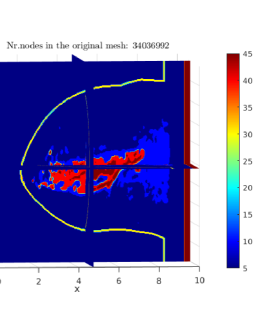
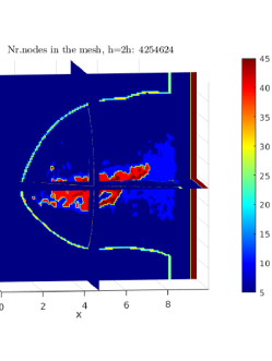
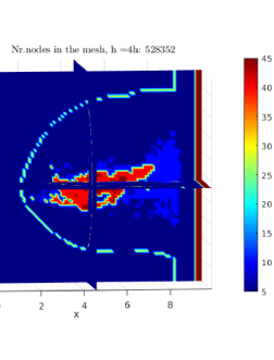
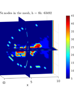
a) b) c) d)

Figure 3:  Spatial distribution of realistic ultrawideband dielectric properties of 3D breast phantom of database [60] developed at the Department of Electrical and Computer Engineering at University of Wisconsin-Madison, USA. Figure a) shows original values of $\varepsilon_{r}$ at 6 GHz for object $ID\_012204$ of database [60]. Figures b)-d) present sampled version of $\varepsilon_{r}$.

$\sigma$

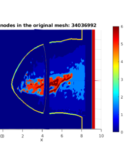
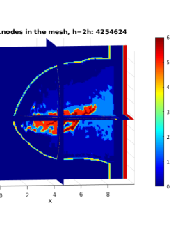
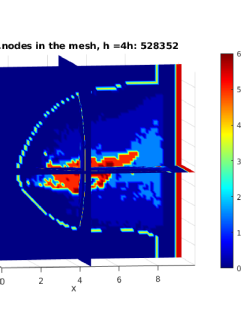
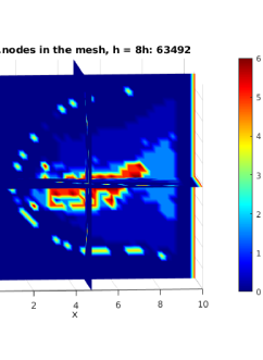
a) b) c) d)

Figure 4:  Spatial distribution of realistic ultrawideband dielectric properties of 3D breast phantom of database [60] developed at the Department of Electrical and Computer Engineering at University of Wisconsin-Madison, USA. Figure a) shows original values of $\sigma$ (S/m) at 6 GHz for object $ID\_012204$ of database [60]. Figures b)-d) present sampled versions of $\sigma$ (S/m).

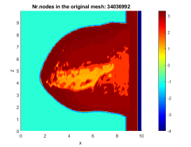
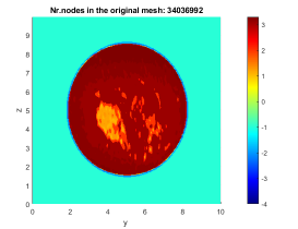
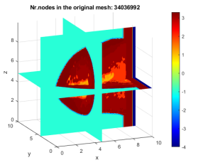
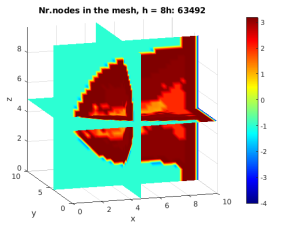
a) $x_{1}x_{3}$ view b) $x_{2}x_{3}$ view c) prospect view d) prospect view

Figure 5:  a)-c) Original values and d) sampled values of the spatial distribution of media numbers of Table 1 for breast phantom of object $ID\_012204$ of database [60]. Table 1 clarifies description of media numbers and corresponding tissue types.

	Media	Test 1	Test 1	Test 2	Test 2
Tissue type	number	$\varepsilon_{r}/5$	$\sigma/5$	$\varepsilon_{r}/5$	$\sigma/5$
Immersion medium	-1	1	0	1	0
Skin	-2	1	0	1	0
Muscle	-4	1	0	1	0
Fibroconnective/glandular-1	1.1	9	1.2	9	1.2
Fibroconnective/glandular-2	1.2	8	1	1	0
Fibroconnective/glandular-3	1.3	8	1	1	0
Transitional	2	1	0	1	0
Fatty-1	3.1	1	0	1	0
Fatty-2	3.2	1	0	1	0
Fatty-3	3.3	1	0	1	0

Table 1: Tissue types and corresponding media numbers of database [60] together with realistic weighted values of $\varepsilon_{r}$ and $\sigma$ (S/m) for breast phantom with ID=012204 used in numerical experiments of section 5.2. Figure 5 presents media numbers of this table on original and sampled meshes.

5.1 Description of anatomically realistic data

We have tested our reconstruction algorithm using three-dimensional realistic breast phantom with ID = 012204 provided in the online repository [60]. The phantom comprises the structural heterogeneity of normal breast tissue for realistic dispersive properties of normal breast tissue at 6 GHz reported in [36, 37]. The breast phantoms of database [60] are derived using T1-weighted MRIs of patients in prone position. Every phantom presents 3D mesh of cubic voxels of the size $0.5\times 0.5\times 0.5$ mm.

Tissue types and corresponding media numbers of breast phantoms are taken from [60] and are given in Table 1. Spatial distribution of these media numbers for phantom with ID = 012204 is presented in Figure 5. Figures 5-a)-c)

demonstrate distribution of media numbers on the original coarse mesh consisting of 34 036 992 nodes. Clearly, performing computations on a such big mesh is computationally demanding task, and thus, we have sampled the original mesh. In all our computations we have used the mesh consisting of 63492 nodes as a coarse finite element mesh which was obtained by taking every 8-th node in $x_{1},x_{2}$ and $x_{3}$ directions of the original mesh. Figures 3-4 shows spatial distribution of dielectric permittivity $\varepsilon_{r}$ and effective conductivity $\sigma$ (S/m) on original and sampled meshes.

Figure 5-d) demonstrates distribution of media numbers on finally sampled mesh. Figure 6 presents spatial distribution of weighted values of $\varepsilon_{r}$ on original and finally sampled mesh for Test 1. Testing of our algorithms on other sampled meshes is computationally expensive task, requiring running of programs in parallel infrastructure, and can be considered as a topic for future research.

We note that in all our computations we scaled original values of $\varepsilon_{r}$ and $\sigma$ of database [60] presented in Figures 3-4 and considered weighted versions of these parameters, in order to satisfy conditions (2) as well as for efficient implementation of FE/FD DDM for solution of forward and adjoint problems. Table 1 presents weighted values of $\varepsilon_{r}$ and $\sigma$ used in numerical tests of this section. Thus, in this way we get computational set-up corresponding to the domain decomposition method which was used in Algorithms 2-5.

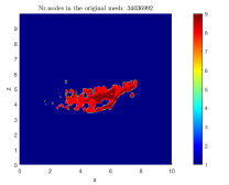
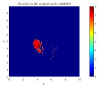
a) $x_{1}x_{3}$ view	b) $x_{2}x_{3}$ view
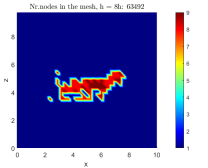
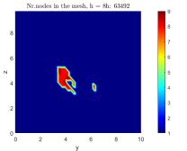
c) $x_{1}x_{3}$ view	d) $x_{2}x_{3}$ view

Figure 6: Test 1. Slices of weighted exact $\varepsilon_{r}$, see Table 1 for description of different tissue types and values of weighted $\varepsilon_{r}$. a), b) Slices on original mesh with mesh size $h$. c), d) Slices on sampled mesh with mesh size $8h$.

Test 1	Test 2
a)	b)

Figure 7: Isosurface of weighted exact dielectric permittivity with value $\varepsilon_{r}\approx 5$ corresponding to tissue type “fibroconnective/glandular-1”: a) In Test 1 and b) In Test 2. Table 1 clarifies description of different tissue types.

5.2 Computational set-up

We have used the domain decomposition Algorithm 2 of section 4.4 to solve forward and adjoint problems in the adaptive reconstruction Algorithm 4. To do this, we set the dimensionless computational domain $\Omega$ as

$$\Omega=\left\{x=(x_{1},x_{2},x_{3})\in(-0.8840,0.8824)\times(-0.8630,0.8648)\times(-0.8945,0.8949)\right\},$$

and the domain $\Omega_{\rm FEM}$ as

$$\Omega_{\rm FEM}=\left\{x=(x_{1},x_{2},x_{3})\in(-0.7,0.6984)\times(-0.7,0.7018)\times(-0.7,0.7004)\right\}.$$

We choose the coarse mesh sizes $h_{1}=0.0368,h_{2}=0.0326,h_{3}=0.0389$ in $x_{1},x_{2},x_{3}$ directions, respectively, in $\Omega=\Omega_{\rm FEM}\cup\Omega_{\rm FDM}$, as well as in the overlapping regions between $\Omega_{\rm FEM}$ and $\Omega_{\rm FDM}$. Corresponding physical domains in meters are $\tilde{\Omega}=0.17664\times 0.17278\times 0.17894$ m for $\Omega$ and $\tilde{\Omega}_{\rm FEM}=0.13985\times 0.14018\times 0.14004$ m for $\Omega_{\rm FEM}$.

The boundary $\partial\Omega$ of the domain $\Omega$ is decomposed into three different parts and is such that $\partial\Omega=\partial_{1}\Omega\cup\partial_{2}\Omega\cup\partial_{3}\Omega$ where $\partial_{1}\Omega$ and $\partial_{2}\Omega$ are, respectively, front and back sides of $\Omega$, and $\partial_{3}\Omega$ is the union of left, right, top and bottom sides of this domain. We will collect time-dependent observations at $\Gamma_{2}:=\partial_{2}\Omega\times(0,T)$, or at the transmitted side $\partial_{2}\Omega$ of $\Omega$. We also define $\Gamma_{1,1}:=\partial_{1}\Omega\times(0,t_{1}]$, $\Gamma_{1,2}:=\partial_{1}\Omega\times(t_{1},T)$, and $\Gamma_{3}:=\partial_{3}\Omega\times(0,T)$.

The following model problem was used in all computations:

$$\begin{split}\frac{1}{c^{2}}\varepsilon_{r}\frac{\partial^{2}E}{\partial t^{2}}+\nabla(\nabla\cdot E)-\triangle E-\varepsilon_{0}\nabla(\nabla\cdot(\varepsilon_{r}E))&=-\mu_{0}\sigma\frac{\partial E}{\partial t}~{}\mbox{in}~{}~{}\Omega_{T},\\ E(x,0)=0,~{}~{}~{}\frac{\partial E}{\partial t}(x,0)&=0~{}\mbox{in}~{}~{}\Omega,\\ \frac{\partial E}{\partial n}&=f(t)~{}\mbox{on}~{}\Gamma_{1,1},\\ \frac{\partial E}{\partial n}&=-\frac{\partial E}{\partial t}~{}\mbox{on}~{}\Gamma_{1,2}\cup\Gamma_{2},\\ \frac{\partial E}{\partial n}&=0~{}\mbox{on}~{}\Gamma_{3}.\\ \end{split}$$ (44)

We initialize a plane wave $f(t)=(0,f_{2},0)(t)$ for one component $E_{2}$ of the electric field $E=(E_{1},E_{2},E_{3})$ at $\Gamma_{1,1}$ in (44). The function $f_{2}(t)$ represents the single direction of a plane wave which is initialized at $\partial_{1}\Omega$ in time $t=[0,3.0]$ and is defined as

$$\begin{split}f_{2}(t)=\left\{\begin{array}[]{ll}\sin\left(\omega t\right),&\text{ if }t\in\left(0,\frac{2\pi}{\omega}\right),\\ 0,&\text{ if }t>\frac{2\pi}{\omega}.\end{array}\right.\end{split}$$ (45)

The goal of our numerical tests Test 1, Test 2 was to reconstruct weighted dielectric permittivity function $\varepsilon_{r}$ shown in Figures 7-a), b). Figures 9-a)-c), 10-a)-c) present simulated solution $|E_{h}|$ in $\Omega_{FEM}$ of model problem (44) for Test 1 and Test 2, correspondingly.

To perform computations for solution of inverse problem, we add normally distributed Gaussian noise with mean $\mu=0$ to simulated electric field at the transmitted boundary $\partial_{2}\Omega$. Then we have smoothed out this data in order to get reasonable reconstructions, see details of data-preprocessing in [52, 53]. Computations of forward and inverse problems were done in time $T=[0,3]$ with equidistant time step $\tau=0.006$ satisfying to CFL condition. Thus, it took $500$ timesteps at every iteration of reconstruction Algorithm 4 to solve forward or adjoint problem. The time interval $T=[0,3]$ was chosen computationally such that the initialized plane wave could reach the transmitted boundary $\partial_{2}\Omega$ in order to obtain meaningful reflections from the object inside the domain $\Omega_{\rm FEM}$. Figures 8-a)-i), 9-a)-c), 10-a)-c) show these reflections in different tests. Experimentally such signals can be produced by a Picosecond Pulse Generator connected with a horn antenna, and scattered time-dependent signals can be measured by a Tektronix real-time oscilloscope, see [52, 53] for details of experimental set-up for generation of a plane wave and collecting time-dependent data. For example, in our computational set-up, the experimental time step between two signals can be $\tilde{\tau}=6$ picoseconds and every signal should be recorded during $\tilde{T}=3$ nanoseconds.

We have chosen following set of admissible parameters for reconstructed function $\varepsilon_{r}(x)$

$$M_{\varepsilon_{r}}=\{\rho\in C^{2}(\overline{\Omega})|1\leq\varepsilon_{r}(x)\leq 10\},$$ (46)

as well as tolerance $\theta=10^{-5}$ at step 3 of the conjugate gradient Algorithm 3. Parameters $\beta_{k}$ in the refined procedure of Algorithm 4 was chosen as the constant $\beta_{k}=0.8$ for all refined meshes ${K_{h}}_{k}$.

a) $t=0.24$	b) $t=0.48$	c) $t=0.72$
d) $t=0.96$	e) $t=1.20$	f) $t=1.44$
g) $t=1.68$	h) $t=1.92$	i) $t=2.16$

Figure 8: The figures a)-i) illustrate how our planar wave $f$ used in implementations propagates through the medium by color plotting $|E_{h}|$ when $\omega=40$, to clarify it’s direction.

$t=1.2$	$t=1.8$	$t=2.4$
a)	b)	c)

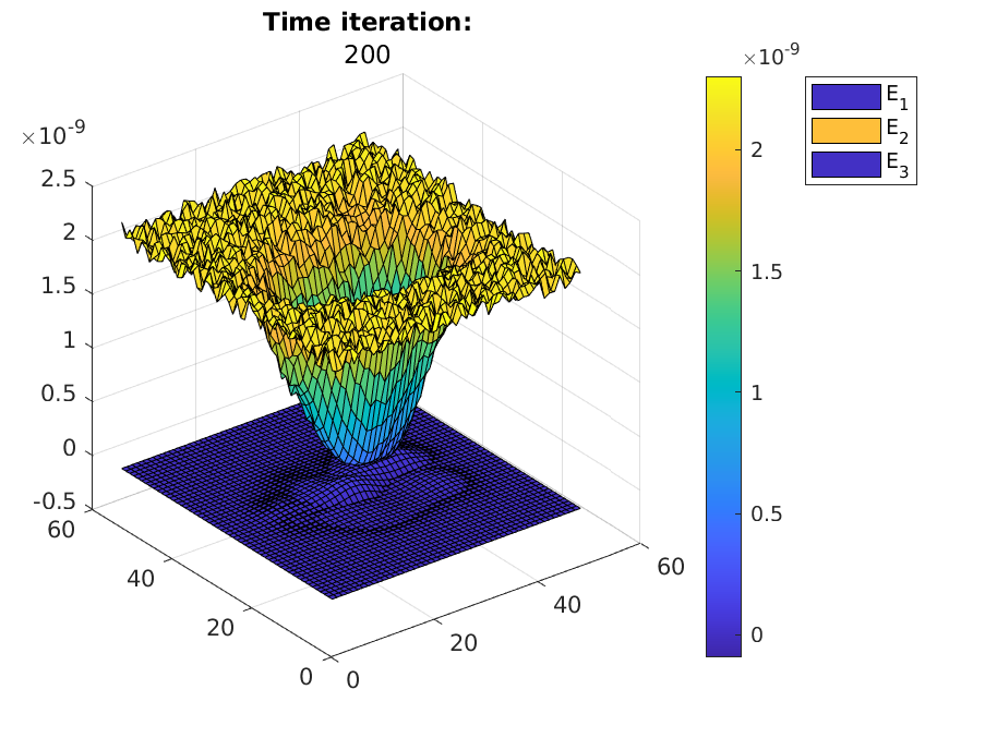
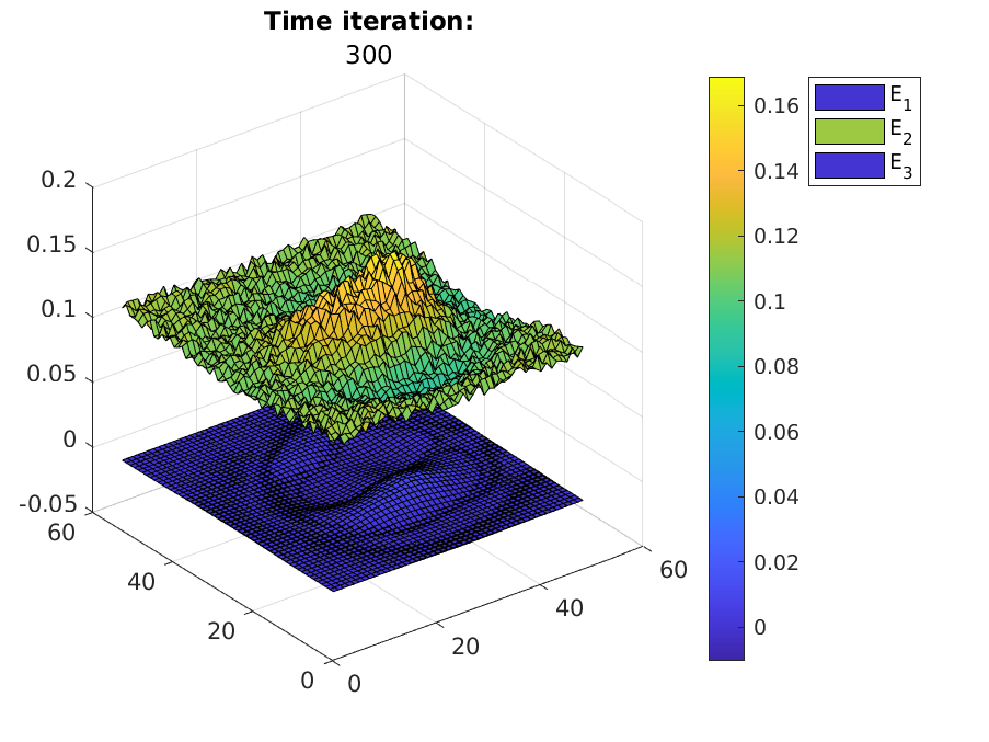
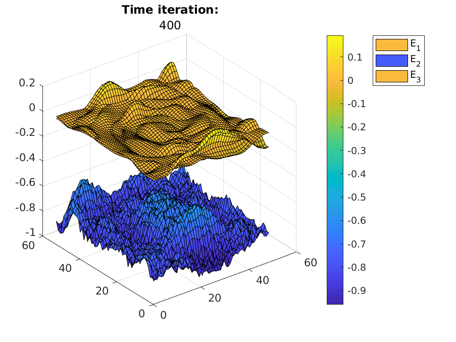
d)	e)	f)

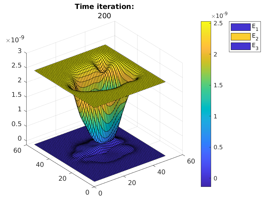
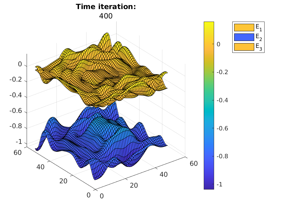
g)	h)	i)

Figure 9: Test 1. a)-c): Solution $|E_{h}|$ of model problem (44) at different times for $\omega=40$ in (45). d)-f): Transmitted noisy scattered data $E_{h}=({E_{1}}_{h},{E_{2}}_{h},{E_{3}}_{h})$ of components of electric field $E=(E_{1},E_{2},E_{3})$ at different times. g)-i): Smoothed transmitted scattered data $E_{h}=({E_{1}}_{h},{E_{2}}_{h},{E_{3}}_{h})$ of components of electric field $E=(E_{1},E_{2},E_{3})$ at different times. The noise level in data is $\delta=10\%$.

$t=1.2$	$t=1.8$	$t=2.4$
a)	b)	c)
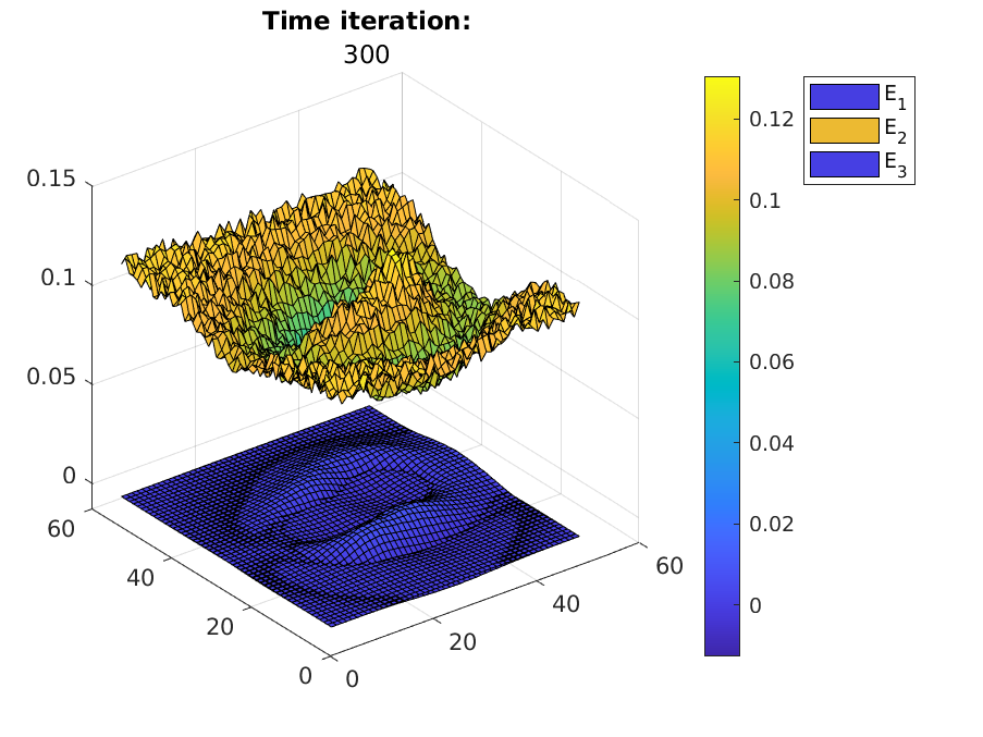
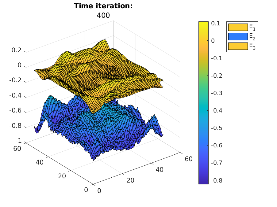
d)	e)	f)
g)	h)	i)

Figure 10: Test 2. a)-c): Solution $|E_{h}|$ of model problem (44) at different times for $\omega=40$ in (45). d)-f): Transmitted noisy scattered data $E_{h}=({E_{1}}_{h},{E_{2}}_{h},{E_{3}}_{h})$ of components of electric field $E=(E_{1},E_{2},E_{3})$ at different times. g)-i): Smoothed transmitted scattered data $E_{h}=({E_{1}}_{h},{E_{2}}_{h},{E_{3}}_{h})$ of components of electric field $E=(E_{1},E_{2},E_{3})$ at different times. The noise level in data is $\delta=10\%$.

Figures 9-d)-i) - 10-d)-i) show simulated data of model problem (44) for all components $(E_{1},E_{2},E_{3})(x,t)$ of electric field $E(x,t)$ at different times at the transmitted boundary $\partial_{2}\Omega$. Figures 9-d)-f) - 10-d)-f) show randomly distributed noisy data and Figures 9-g)-i) - 10-g)-i) show smoothed noisy data used for solution of inverse problem.

These figures show that largest by amplitude reflections, or transmitted data, are obtained from the second component $E_{2}$ of the electric field $E$. The same observation is obtained in previous works [4, 12] where was used a similar computational set-up with a plane wave. However, comparison of all three components was not presented in [12]. Domination of reflections at the transmitted boundary from the $E_{2}$ component can be explained by the fact that we initialize only one component of the electric field $E=(E_{1},E_{2},E_{3})$ as a plane wave $f(t)=(0,f_{2},0)(t)$ at $\Gamma_{1,1}$ in the model problem (44), and thus, two other components $E_{1},E_{3}$ will be smaller by amplitude than the $E_{2}$ when we use the explicit scheme (29) for computations. See also theoretical justification of this fact in [51].

Numerical tests of [12] show that the best reconstruction results of the space-dependent function $\varepsilon_{r}(x)$ for $\sigma=0$ in $\Omega$ are obtained for $\omega=40$ in (45). Thus, we performed simulations of the forward problem (44) taking $\sigma=0$ for different $\omega=40,60,80,100$ in (45). It turned out that for chosen computational set-up with final time $T=3$ maximal values of scattered function $E_{2}$ are obtained for $\omega=40$. Thus, we take $\omega=40$ in (45) in all our tests.

We assume that both functions $\varepsilon_{r},\sigma$ satisfy conditions (2): they are known inside $\Omega_{\rm out}\cup\Omega_{\rm FDM}$ and unknown inside $\Omega_{IN}$. The goal of our numerical tests is to reconstruct the function $\varepsilon_{r}$ of the domain $\Omega_{\rm FEM}$ of Figure 7 under conditions (2) and the additional condition that the function $\sigma(x)$ of this domain is known. See Table 1 for distribution of $\varepsilon_{r},\sigma$ in $\Omega_{\rm FEM}$.

The computational set-up for solution of inverse problem is as follows. We generate transmitted data by solving the model problem (44) on three times adaptively refined mesh. In this way we avoid variational crimes when we solve the inverse problem. The transmitted data is collected at receivers located at every point of the transmitted boundary $\partial_{2}\Omega$, and then normally distributed Gaussian noise $\delta=3\%,10\%$ with mean $\mu=0$ is added to this data, see Figures 9-d)-f) - 10-d)-f). The next step is data pre-processing: the noisy data is smoothed out, see Figures 9-g)-i) - 10-g)-i). Next, to reconstruct $\varepsilon_{r}$ we minimize the Tikhonov functional (8). For solution of the minimization problem we introduce Lagrangian and search for a stationary point of it using an adaptive Algorithm 4, see details in section 4.6.

We take the initial approximation $\varepsilon_{0}=1$ at all points of the computational domain what corresponds to starting of our computations from the homogeneous domain. This is done because of previous computational works [12] as well as experimental works of [38, 32, 50] where was shown that a such choice gives good results of reconstruction of dielectric permittivity function.

Test 1 $\delta=3\%$ $\delta=10\%$ Mesh $\max_{\Omega_{\rm FEM}}{\varepsilon_{h}}_{k}$ $\frac{\max_{\Omega_{\rm FEM}}|\varepsilon_{r}-{\varepsilon_{h}}_{k}|}{\max_{\Omega_{\rm FEM}}|\varepsilon_{r}|}$ $M^{k}$ ${K_{h}}_{0}$ 6.535 0.274 2 ${K_{h}}_{1}$ 7.865 0.126 2 ${K_{h}}_{2}$ 10.0 0.111 2 Mesh $\max_{\Omega_{\rm FEM}}{\varepsilon_{h}}_{k}$ $\frac{\max_{\Omega_{\rm FEM}}|\varepsilon_{r}-{\varepsilon_{h}}_{k}|}{\max_{\Omega_{\rm FEM}}|\varepsilon_{r}|}$ $M^{k}$ ${K_{h}}_{0}$ 7.019 0.220 2 ${K_{h}}_{1}$ 7.481 0.167 4 ${K_{h}}_{2}$ 9.234 0.026 4

Table 2: Test 1. Computational results of the reconstructions $\max_{\Omega_{\rm FEM}}{\varepsilon_{h}}_{k}$ on a coarse and on adaptively refined meshes together with relative errors computed in the maximal contrast of $\max_{\Omega_{\rm FEM}}\varepsilon_{r},\max_{\Omega_{\rm FEM}}{\varepsilon_{h}}_{k}$. Here, $\max_{\Omega_{\rm FEM}}{\varepsilon_{h}}_{k}$ denotes maximum of the computed function $\varepsilon_{h}$ on $k$ times refined mesh ${K_{h}}_{k}$ in the domain $\Omega_{\rm FEM}$, and $M^{k}$ denotes the final number of iterations in the conjugate gradient Algorithm 3 on $k$ times refined mesh ${K_{h}}_{k}$ for reconstructed function ${\varepsilon_{h}}_{k},k=0,1,2$.

Test 1, Computational Time $\delta=3\%$ $\delta=10\%$ Mesh nno Time (sec) Rel. time $M^{k}$ ${K_{h}}_{0}$ 63492 1183 3.73 $\cdot 10^{-5}$ 2 ${K_{h}}_{1}$ 64206 1199 3.74 $\cdot 10^{-5}$ 2 ${K_{h}}_{2}$ 65284 1212 3.71 $\cdot 10^{-5}$ 2 Mesh nno Time (sec) Rel. time $M^{k}$ ${K_{h}}_{0}$ 63492 1180 $3.71\cdot 10^{-5}$ 2 ${K_{h}}_{1}$ 64766 2415 $7.43\cdot 10^{-5}$ 4 ${K_{h}}_{2}$ 67965 2525 $7.435\cdot 10^{-5}$ 4

Table 3: Test 1. Performance of the reconstruction Algorithm 4 (in seconds) on adaptively refined meshes. Here, $k$ is number of the refined mesh ${K_{h}}_{k}$ of the domain $\Omega_{\rm FEM}$, ${\rm nno}$ is number of the nodes in the computational mesh ${K_{h}}_{k}$, and $M^{k}$ denotes the final number of iterations in the conjugate gradient Algorithm 3.

a) perspective view	b) $x_{1}x_{2}$ view	c) $x_{2}x_{3}$ view
d) perspective view	e) $x_{1}x_{2}$ view	f) $x_{2}x_{3}$ view
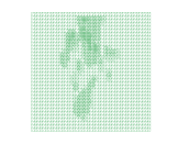
g) $x_{1}x_{3}$ view	h) $x_{1}x_{2}$ view	i) $x_{2}x_{3}$ view

Figure 11: Test 1. a)-c): Reconstructions $\varepsilon_{h_{0}}\approx 5$ (outlined in transparent green color) of $\varepsilon_{r}$ obtained on the coarse mesh. d)-f): Reconstructions ${\varepsilon_{h}}_{2}\approx 5$ obtained on refined mesh ${K_{h}}_{2}$. g) - i): refined mesh ${K_{h}}_{2}$. The noise level in the data is $\delta=10\%$. See Table 2 for obtained contrasts $\max_{\Omega_{\rm FEM}}{\varepsilon_{h}}_{k},k=0,1,2$. For comparison we also present exact isosurface with value corresponding to reconstructed one and outlined by red color.

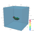
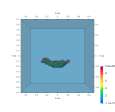
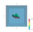
a) prospect view	b) $x_{1}x_{2}$ view	c) $x_{1}x_{3}$ view
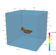
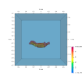
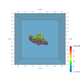
d) prospect view	e) $x_{1}x_{2}$ view	f) $x_{1}x_{3}$ view
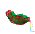
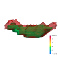
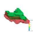
g) zoomed prospect view	h) zoomed $x_{1}x_{2}$ view	i) zoomed $x_{1}x_{3}$ view
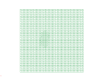
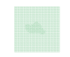
j) $x_{2}x_{3}$ view	k) $x_{1}x_{2}$ view	l) $x_{1}x_{3}$ view

Figure 12: Test 2. a) -c): Isosurfaces of reconstructions $\varepsilon_{h_{0}}\approx 5$ (in green color) of $\varepsilon_{r}$ obtained on the coarse mesh ${K_{h}}_{0}$. d)-f): Isosurfaces of reconstructions ${\varepsilon_{h}}_{1}\approx 5$ obtained on refined mesh ${K_{h}}_{1}$ (in yellow color). g)-i) Zoomed reconstructions. j) -l): Refined mesh ${K_{h}}_{1}$. The noise level in the data is $\delta=10\%$. See Table 4 for obtained contrasts $\max_{\Omega_{\rm FEM}}{\varepsilon_{h}}_{k},k=0,1$. For comparison we also present exact isosurface of $\varepsilon_{r}$ with value corresponding to reconstructed one and outlined by red color.

5.3 Test 1

In this test we present numerical results of reconstruction of $\varepsilon_{r}$ when exact values of this function are given in Table 1, see Test 1. Isosurface of the exact function $\varepsilon_{r}$ to be reconstructed in this test is shown in Figure  7-a). We note that the exact function $\varepsilon_{r}$ has complicated structure. Using Figure  7-a) one can observe that isosurface presents a discontinuous function with a lot of big and small inclusions in the domain $\Omega_{\rm FEM}$.

Figures 11-a)-i) show results of the reconstruction on adaptively locally refined meshes when noise level in the data was $\delta=10\%$. We start computations on a coarse mesh ${K_{h}}_{0}$. Figure 11-a)-c) shows that the location of the reconstructed function ${\varepsilon_{h}}_{0}$ is imaged correctly and the reconstructed isosurface covers the domain where the exact $\varepsilon_{r}$ is located. We refer to Table 2 for the reconstruction of the maximal contrast in ${\varepsilon_{h}}_{0}$. For improvement of the contrast and shape obtained on a coarse mesh ${K_{h}}_{0}$, we run computations on locally adaptivelly refined meshes. Figures 11-d)-f) show reconstruction obtained on the final two times refined mesh ${K_{h}}_{2}$. Table 2 presents results of reconstructions for ${\varepsilon_{h}}_{k}$ obtained on the refined meshes ${K_{h}}_{k},k=0,1,2$. We observe that with mesh refinements we achieve better contrast for function $\varepsilon_{r}$. Also reconstructed isosurface of this function more precisely covers the domain where the exact $\varepsilon_{r}$ is located, compare Figure 11-a) with Figure 11-d). Figures 11-g)-i) show locally adaptively refined mesh ${K_{h}}_{2}$.

Test 2 $\delta=3\%$ $\delta=10\%$ Mesh $\max_{\Omega_{\rm FEM}}{\varepsilon_{h}}_{k}$ $\frac{\max_{\Omega_{\rm FEM}}|\varepsilon_{r}-{\varepsilon_{h}}_{k}|}{\max_{\Omega_{\rm FEM}}|\varepsilon_{r}|}$ $M^{k}$ ${K_{h}}_{0}$ 6.874 0.236 2 ${K_{h}}_{1}$ 7.558 0.160 5 ${K_{h}}_{2}$ 10.0 0.111 2 Mesh $\max_{\Omega_{\rm FEM}}{\varepsilon_{h}}_{k}$ $\frac{\max_{\Omega_{\rm FEM}}|\varepsilon_{r}-{\varepsilon_{h}}_{k}|}{\max_{\Omega_{\rm FEM}}|\varepsilon_{r}|}$ $M^{k}$ ${K_{h}}_{0}$ 5.350 0.406 2 ${K_{h}}_{1}$ 9.450 0.05 4

Table 4: Test 2. Computational results of the reconstructions $\max_{\Omega_{\rm FEM}}{\varepsilon_{h}}_{k}$ on a coarse and on adaptively refined meshes together with relative errors computed in the maximal contrast of $\max_{\Omega_{\rm FEM}}\varepsilon_{r},\max_{\Omega_{\rm FEM}}{\varepsilon_{h}}_{k}$. Here, $\max_{\Omega_{\rm FEM}}{\varepsilon_{h}}_{k}$ denotes maximum of the computed function $\varepsilon_{h}$ on $k$ times refined mesh ${K_{h}}_{k}$ in the domain $\Omega_{\rm FEM}$, and $M^{k}$ denotes the final number of iterations in the conjugate gradient Algorithm 3 on $k$ times refined mesh ${K_{h}}_{k}$ for reconstructed function ${\varepsilon_{h}}_{k},k=0,1,2$.

Test 2, Computational Time $\delta=3\%$ $\delta=10\%$ Mesh nno Time (sec) Rel. time $M^{k}$ ${K_{h}}_{0}$ 63492 1186 3.72 $\cdot 10^{-5}$ 2 ${K_{h}}_{1}$ 64096 3588 9.34 $\cdot 10^{-5}$ 5 ${K_{h}}_{2}$ 66112 1228 3.72 $\cdot 10^{-5}$ 2 Mesh nno Time (sec) Rel. time $M^{k}$ ${K_{h}}_{0}$ 63492 1214 $3.82\cdot 10^{-5}$ 2 ${K_{h}}_{1}$ 63968 2384 $7.44\cdot 10^{-5}$ 4

Table 5: Test 2. Performance of the reconstruction Algorithm 4 (in seconds) on adaptively refined meshes. Here, $k$ is number of the refined mesh ${K_{h}}_{k}$ of the domain $\Omega_{\rm FEM}$, ${\rm nno}$ is number of the nodes in the computational mesh ${K_{h}}_{k}$, and $M^{k}$ denotes the final number of iterations in the conjugate gradient Algorithm 3.

5.4 Test 2

Since it is quite demanding reconstruct very complicated structure of $\varepsilon_{r}$ taken in Test 1, in this test we will reconstruct $\varepsilon_{r}$ with exact isosurface as it is presented in the Figure 7-b). Exact values of this function are taken as in fibroconnective/glandular-1 media (see Table 1) inside isosurface of Figure 7-b), and outside of this isosurface all values of $\varepsilon_{r}=1$.

Figures 12-a)-i) show results of the reconstruction on adaptively refined meshes when noise level in the data was $\delta=10\%$. We refer to the Table 4 for reconstruction of the contrast in $\varepsilon_{r}$. Using the Table 4 we now observe that with mesh refinements we achieve slightly higher maximal contrast $9.45$ in reconstruction ${\varepsilon_{h}}_{1}$ compared to the exact one $9$. Moreover, on the mesh ${K_{h}}_{1}$ for $\sigma=10\%$ we get more than 8 times smaller relative error in the reconstruction compared to the error obtained on the coarse mesh ${K_{h}}_{0}$. Figures 12-d)-i) show good matching of the reconstructed ${\varepsilon_{h}}_{1}$ compared with the exact one. Figures 11-j)-l) show locally adaptively refined mesh ${K_{h}}_{2}$.

Computational time $\delta=3\%$ $\delta=10\%$ Time (sec) Relative time $n$ Test 1 110.59 $1.779\cdot 10^{-6}$ 71360 Test 2 106.58 $1.714\cdot 10^{-6}$ 69699 Time (sec) Relative time $n$ Test 1 116.22 $1.869\cdot 10^{-6}$ 75052 Test 2 111.53 $1.793\cdot 10^{-6}$ 65359

Table 6: Performance of solution of forward problem (44) in Tests 1 and 2 of section 5 on the mesh ${K_{h}}_{0}$ in terms of computational time (in seconds) and relative computational time computed by (47). Here, $n$ is number of the nodes on three times adaptively refined original coarse mesh (consisting of 63492 nodes) which we used for generation of transmitted data.

5.5 Performance comparison

All computations were performed on a linux workstation Intel Core i7-9700 CPU with one processor using software package WavES [58] efficiently implemented in C++/PETSc [49].

We have estimated the relative computational time $T_{r}$ of the forward problem using the following formula

$$T_{r}=\frac{t}{n_{t}\cdot n}.$$ (47)

Here, $t$ is the total computational time of the forward problem on the mesh ${K_{h}}_{l}$ where $l=0,1,2,...$ is number of the refined mesh, $n$ is the total number of nodes in the mesh ${K_{h}}_{l}$, $n_{t}$ is number of timesteps. We take $n_{t}=500$ in all computational tests, see clarification in section 5.2. Computational times (in seconds) for solution of forward problem are presented in Table 6. Using this table we observe that the relative time is approximately the same for all tests and we can take it as $T_{r}\approx 1.8\cdot 10^{-6}$. Next, using this relative time we can estimate approximate computational time for solution of forward problem for any mesh consisting of $n$ nodes. For example, if we will take original mesh consisting of $n=34036992$ nodes, then computational time will be already $t=T_{r}\cdot n_{t}\cdot n=1.8\cdot 10^{-6}\cdot 500\cdot 34036992=30633$ seconds, and this time is not computationally efficient. Clearly, computing of the solution of inverse problem on the sampled mesh allows significantly reduce computational times.

We have estimated also the relative computational time $T_{r}^{ip}$ of the solution of inverse problem using the formula

$$T_{r}^{ip}=\frac{t^{ip}}{n_{t}\cdot nno}.$$ (48)

Here, $t^{ip}$ is the total computational time to run inverse Algorithm 4 on the mesh ${K_{h}}_{l}$ where $l=0,1,2,...$ is number of the refined mesh, $nno$ is the total number of nodes in the mesh ${K_{h}}_{l}$, $n_{t}$ is number of timesteps. Computational times (in seconds) for solution of inverse problem for Test 1 and Test 2 are presented in Tables 3,5, respectivelly. Using these tables we observe that computational times are depend on the number of iterations $M^{k}$ in the conjugate gradient method (CGM) and number of the nodes $nno$ in the meshes ${K_{h}}_{l}$. We took $n_{t}=500$ for all tests and thus, computational times presented in these tables are not depend on number of times steps for different refined meshes. We note, that the number of time steps $n_{t}$ can be chosen adaptively as well. However, we are performing only adaptive mesh refinement in space and not in time. The full space-time adaptive algorithm can be considered as a topic for future research.

Using Table 3 we observe that computational time in Test 1 is around 20 minutes for both noise levels $\sigma=3\%$ and $\sigma=10\%$. On every mesh ${K_{h}}_{l},l=0,1,2$, was performed two iterations CGM , or $M^{K}=2$. Thus, the total computational time to obtain final reconstruction in Test 1 is 60 min.

Table 5 shows that computational time in Test 2 with noise in data $\delta=3\%$ is around 20 minutes for non-refined mesh ${K_{h}}_{0}$, 60 min for one time refined mesh ${K_{h}}_{1}$, and 20 minutes for twice refined mesh ${K_{h}}_{2}$. Thus, the total computational time to obtain final reconstruction in Test 2 is 100 minutes. Computational time in this test is larger than in the previous Test 1 since CGM converged only at 5-th iteration on the one time refined mesh ${K_{h}}_{1}$. However, the total computational time with noise in data $\delta=10\%$ is around 60 minutes. This is because the solution was obtained already on the one time refined mesh ${K_{h}}_{1}$. Tables 3, 5 also demonstrate that it takes around 10 minutes to compute solution of inverse problem on the one iteration of the conjugate gradient algorithm.

We note that PETSc supports parallel implementation and thus, current version of code can be extended to the version with parallel implementation such that times reported in Tables 6, 3 and Table 5 can be significantly reduced.

6 Conclusions

This work describes reconstruction methods for determination of the relative dielectric permittivity function in conductive media using scattered data of the time-dependent electric field at number of detectors placed at the boundary of the investigated domain.

Reconstruction methods use optimization approach where a functional is minimized via a domain decomposition finite element/finite difference method. In an adaptive reconstruction method the space mesh is refined only in the domain where a finite element method is used with a feedback from a posteriori error indicators. Developed adaptive algorithms allow us to obtain correct values and shapes of the dielectric permittivity function to be determined. Convergence and stability analysis of the developed methods is ongoing work and will be presented in forthcoming publication. The algorithms of the current work are designed from previous adaptive algorithms developed in [8, 12] which reconstruct the wave speed or the dielectric permittivity function. However, all previous algorithms are developed for non-conductive medium.

Our computational tests show qualitative and quantitative reconstruction of dielectric permittivity function using anatomically realistic breast phantom which capture the heterogeneity of normal breast tissue at frequency 6 GHz taken from online repository [60]. In all tests we used assumption that the conductivity function is known. Currently we are working on algorithms when both dielectric permittivity and conductivity functions can be reconstructed. Results of this work will be presented in our future research.

All computations are performed in real time presented in Tables 3, 5 and 6. Some data (Matlab code to read data of database [60], visualize and produce discretized values of $\varepsilon_{r},\sigma$, etc.) used in computations of this work is available for download and testing, see [59]. Additional data (computational FE/FD meshes, transmitted data, C++/PETSc code) can be provided upon request.

In summary, the main features of algorithms of this work are as follows:

• Ability to reconstruct shapes, locations and maximal values of dielectric permittivity function of targets in conductive media under the condition that the conductivity of this media is a known function.

• More exact reconstruction of shapes and maximal values of dielectric permittivity function of inclusions because of local adaptive mesh refinement.

• Computational greater efficiency because of usage software package WavES [58] implemented in C++/PETSc [49].

References

- [1]
- [2] M. G. Aram, L. Beilina, H. Dobsicek Trefna, Microwave Thermometry with Potential Application in Non-invasive Monitoring of Hyperthermia, Journal of Inverse and Ill-posed problems, 2020.
- [3] A. B. Bakushinsky and M. Yu. Kokurin, Iterative Methods for Approximate Solution of Inverse Problems, Springer, Dordrecht, The Netherlands, 2004.
- [4] L. Beilina, Energy estimates and numerical verification of the stabilized Domain Decomposition Finite Element/Finite Difference approach for time-dependent Maxwell’s system, Cent. Eur. J. Math., 11 (2013), 702-733 DOI: 10.2478/s11533-013-0202-3.
- [5] L. Beilina, V. Ruas, Convergence of Explicit P1 Finite-Element Solutions to Maxwell’s Equations, Springer Proceedings in Mathematics and Statistics, vol 328. Springer, Cham (2020)
- [6] L. Beilina, V. Ruas, An explicit P1 finite element scheme for Maxwell’s equations with constant permittivity in a boundary neighborhood, arXiv:1808.10720
- [7] L. Beilina and M. V. Klibanov, Approximate global convergence and adaptivity for Coefficient Inverse Problems, Springer, New York, 2012.
- [8] L. Beilina, N. T. Th‘anh, M.V. Klibanov and J. B. Malmberg, Globally convergent and adaptive finite element methods in imaging of buried objects from experimental backscattering radar measurements, Journal of Computational and Applied Mathematics, Elsevier, DOI: 10.1016/j.cam.2014.11.055, 2015.
- [9] M. I. Belishev, Boundary control in reconstruction of manifolds and metrics (the bc method), Inverse Problems, 13 (1997), pp. R1-R45.
- [10] M. I. Belishev and V. Y. Gotlib, Dynamical variant of the bc-method: Theory and numerical testing, J. Inverse Ill-Posed Prob., 7 (1999), pp. 221-240.
- [11] S. C. Brenner and L. R. Scott, The Mathematical Theory of Finite Element Methods, Springer-Verlag, Berlin, 1994.
- [12] J. Bondestam Malmberg, L. Beilina, An Adaptive Finite Element Method in Quantitative Reconstruction of Small Inclusions from Limited Observations, Appl. Math. Inf. Sci., 12(1), 1-19, 2018.
- [13] V. A. Burov, S. A. Morozov, and O. D. Rumyantseva, Reconstruction of fine-scale structure of acoustical scatterers on large-scale contrast background, Acoustical Imaging, 26 (2002), pp. 231-238.
- [14] Y. Chen, Inverse scattering via Heisenberg uncertainty principle, Inverse Problems, 13 (1997), pp. 253-282.
- [15] G. C. Cohen, Higher Order Numerical Methods for Transient Wave Equations, Springer-Verlag, Berlin, 2002.
- [16] A. E. Bulyshev, A. E. Souvorov, S. Y. Semenov, V. G. Posukh and Y. E. Sizov, Three-dimensional vector microwave tomography: theory and computational experiments, Inverse Problems, 20(4), pp.1239-1259, 2004.
- [17] T. Chan and T. Mathew, Domain decomposition algorithms, In A. Iserles, editor, Acta Numerica, 3, Cambridge University Press, Cambridge, 1994.
- [18] W. C. Chew, Y. M. Wang, Reconstruction of two-dimensional permittivity distribution using the distorted Born iterative method, IEEE Trans. Med. Imaging, 9(2), pp. 218-225, 1990.
- [19] Cuccaro, A.; Dell’Aversano, A.; Ruvio, G.; Browne, J.; Solimene, R. Incoherent Radar Imaging for Breast Cancer Detection and Experimental Validation against 3D Multimodal Breast Phantoms. Journal of Imaging 2021, 7, 23. https://doi.org/10.3390/jimaging7020023
- [20] Solimene, R.; Cuccaro, A.; Ruvio, G.; Tapia, D.F.; Halloran, M.O. Beamforming and Holography Image Formation Methods: An Analytic Study. Optics Express, 2016, 24, 9077–9093.
- [21] A. Elmkies and P. Joly, Finite elements and mass lumping for Maxwell’s equations: the 2D case. Numerical Analysis, C. R. Acad.Sci.Paris, 324, pp. 1287–1293, 1997.
- [22] H. W. Engl, M. Hanke, and A. Neubauer, Regularization of Inverse Problems, Kluwer Academic Publishers, Dordrecht, The Netherlands, 1996.
- [23] B. Engquist and A. Majda, Absorbing boundary conditions for the numerical simulation of waves, Math. Comp., 31, 629-651, 1977.
- [24] G. Chavent, Nonlinear Least Squares for Inverse Problems. Theoretical Foundations and Step-by- Step Guide for Applications, Springer, New York, 2009.
- [25] A. V. Goncharsky, S. Y. Romanov, A method of solving the coefficient inverse problems of wave tomography, Comput. Math. Appl., 2019;77:967–980.
- [26] A. V. Goncharsky, S. Y. Romanov, S. Y. Seryozhnikov, Low-frequency ultrasonic tomography: math- ematical methods and experimental results. Moscow University Phys Bullet. 2019;74(1): 43–51.
- [27] B. Jiang, The Least-Squares Finite Element Method. Theory and Applications in Computational Fluid Dynamics and Electromagnetics, Springer-Verlag, Heidelberg, 1998.
- [28] B. Jiang, J. Wu and L. A. Povinelli, The origin of spurious solutions in computational electromagnetics, Journal of Computational Physics, 125, pp.104–123, 1996.
- [29] J. Jin, The finite element method in electromagnetics, Wiley, 1993.
- [30] P. Joly, Variational methods for time-dependent wave propagation problems, Lecture Notes in Computational Science and Engineering, Springer, 2003.
- [31] W.T. Joines, Y. Zhang, C. Li, and R. L. Jirtle, The measured electrical properties of normal and malignant human tissues from 50 to 900 MHz’, Med. Phys., 21 (4), pp.547-550, 1994.
- [32] N. Joachimowicz, C. Pichot and J. P. Hugonin, Inverse scattering: and iterative numerical method for electromagnetic imaging, IEEE Trans. Antennas Propag., 39(12), pp.1742-1753, 1991.
- [33] S. Kabanikhin, A. Satybaev, and M. Shishlenin, Direct Methods of Solving Multidimensional Inverse Hyperbolic Problems, VSP, Ultrecht, The Netherlands, 2004.
- [34] M.V. Klibanov and J. Li, Inverse Problems and Carleman Estimates: Global Uniqueness, Global Convergence and Experimental Data, De Gruyter, 2021.
- [35] M. Křížek, P. Neittaanmäki: Finite element approximation of variational problems and applications, Longman, Harlow, 1990.
- [36] M. Lazebnik, L. McCartney, D. Popovic, C. B. Watkins, M. J. Lindstrom, J. Harter, S. Sewall, A. Magliocco, J. H. Booske, M. Okoniewski, and S. C. Hagness, A large-scale study of the ultrawideband microwave dielectric properties of normal breast tissue obtained from reduction surgeries, Physics in Medicine and Biology, vol. 52, pp. 2637-2656, April 2007.
- [37] M. Lazebnik, D. Popovic, L. McCartney, C. B. Watkins, M. J. Lindstrom, J. Harter, S. Sewall, T. Ogilvie, A. Magliocco, T. M. Breslin, W. Temple, D. Mew, J. H. Booske, M. Okoniewski, and S. C. Hagness, A large-scale study of the ultrawideband microwave dielectric properties of normal, benign, and malignant breast tissues obtained from cancer surgeries, Physics in Medicine and Biology, 52(20):6093-115, 2007. doi: 10.1088/0031-9155/52/20/002
- [38] T.M. Grzegorczyk, P.M. Meaney, P.A. Kaufman, R.M. diFlorio Alexander, and K.D. Paulsen, Fast 3-d tomographic microwave imaging for breast cancer detection, IEEE Trans Med Imaging, 31:1584–1592, 2012.
- [39] Vo Anh Khoa, Grant W. Bidney, Michael V. Klibanov, Loc H. Nguyen, Lam H. Nguyen, Anders J. Sullivan & Vasily N. Astratov (2021), An inverse problem of a simultaneous reconstruction of the dielectric constant and conductivity from experimental backscattering data, Inverse Problems in Science and Engineering, 29:5, 712-735, DOI: 10.1080/17415977.2020.1802447
- [40] J. Mueller and S. Siltanen, Direct reconstructions of conductivities from boundary measurements, SIAM J. Sci. Comp., 24 (2003), pp. 1232-1266.
- [41] P. B. Monk, Finite Element methods for Maxwell’s equations, Oxford University Press, 2003.
- [42] P. B. Monk and A. K. Parrott, A dispersion analysis of finite element methods for Maxwell’s equations, SIAM J.Sci.Comput., 15, pp.916–937, 1994.
- [43] C. D. Munz, P. Omnes, R. Schneider, E. Sonnendrucker and U. Voss, Divergence correction techniques for Maxwell Solvers based on a hyperbolic model, Journal of Computational Physics, 161, pp.484–511, 2000.
- [44] J.-C. Nédélec, Mixed finite elements in R3, Numerische Mathematik, 35 (1980), 315-341.
- [45] A. Nachman, Global uniqueness for a two-dimensional inverse boundary value problem, Ann. of Math., 143 (1996), pp. 71-96.
- [46] R. G. Novikov, The approach to approximate inverse scattering at fixed energy in three dimensions, Internat. Math. Res. Papers, 6 (2005), pp. 287-349.
- [47] K. D. Paulsen, D. R. Lynch, Elimination of vector parasites in Finite Element Maxwell solutions, IEEE Transactions on Microwave Theory Technologies, 39, 395 –404, 1991.
- [48] O.Pironneau, Optimal Shape Design for Elliptic Systems, Springer-Verlag, Berlin, 1984.
- [49] Portable, Extensible Toolkit for Scientific Computation PETSc, http://www.mcs.anl.gov/petsc/
- [50] Poplack S. P., Tosteson T. D., Wells W. A., Pogue B. W., Meaney P. M., Hartov A., Kogel C. A., Soho S. K., Gibson J. J., and Paulsen K. D., Electromagnetic Breast Imaging: Results of a Pilot Study in Women with Abnormal Mammograms. Radiology, 243(2):350-359, May 2007.
- [51] V. G. Romanov, M. V. Klibanov, Can a single PDE govern well the propagation of the electric wave field in a heterogeneous medium in 3D? https://arxiv.org/abs/2102.02271
- [52] N. T. Thánh, L. Beilina, M. V. Klibanov, and M. A. Fiddy, Reconstruction of the refractive index from experimental backscattering data using a globally convergent inverse method, SIAMJ. Sci. Comput., 36 (2014), pp. B273-B293.
- [53] N. T. Thánh, L. Beilina, M. V. Klibanov, M. A. Fiddy, Imaging of Buried Objects from Experimental Backscattering Time-Dependent Measurements using a Globally Convergent Inverse Algorithm, SIAM Journal on Imaging Sciences, 8(1), 757-786, 2015.
- [54] A. N. Tikhonov, A. V. Goncharsky, V. V. Stepanov and A. G. Yagola, Numerical Methods for the Solution of Ill-Posed Problems, London, Kluwer, 1995.
- [55] A. Toselli and B. Widlund, Domain Decomposition Methods, Springer, Berlin, 2005.
- [56] K. Ito, B. Jin, Inverse Problems: Tikhonov theory and algorithms, Series on Applied Mathematics, V.22, World Scientific, 2015.
- [57] X. Zeng, A. Fhager, Z. He, M. Persson, P. Linner, H. Zirath, Development of a Time Domain Microwave System for Medical Diagnostics, IEEE Trans. on Instrumentation and Measurement, 63(12), 2014.
- [58] WavES, the software package, http://www.waves24.com/
- [59] WavES, DD FEM/FDM for time-dependent Maxwell’s equations, data repository github.com/ProjectWaves24/DDFEMFDMMaxwell
- [60] E. Zastrow, S. K. Davis, M. Lazebnik, F. Kelcz, B. D. Veen, S. C. Hageness, Online repository of 3D Grid Based Numerical Phantoms for use in Computational Electromagnetics Simulations, https://uwcem.ece.wisc.edu/MRIdatabase/