Full-band General Audio Synthesis with Score-based Diffusion

Abstract

Recent works have shown the capability of deep generative models to tackle general audio synthesis from a single label, producing a variety of impulsive, tonal, and environmental sounds. Such models operate on band-limited signals and, as a result of an autoregressive approach, they are typically conformed by pre-trained latent encoders and/or several cascaded modules. In this work, we propose a diffusion-based generative model for general audio synthesis, named DAG, which deals with full-band signals end-to-end in the waveform domain. Results show the superiority of DAG over existing label-conditioned generators in terms of both quality and diversity. More specifically, when compared to the state of the art, the band-limited and full-band versions of DAG achieve relative improvements that go up to 40 and 65%, respectively. We believe DAG is flexible enough to accommodate different conditioning schemas while providing good quality synthesis.

Index Terms—  Deep generative models, audio synthesis, full-band audio, score-based diffusion, Fréchet distance.

1 Introduction

Audio synthesis is the computerized generation of audio signals. This task has been primarily tackled under a source-specific paradigm, hence modeling a single type of audio per model. Examples of this paradigm are text-to-speech [1], music synthesis [2, 3, 4], or less commonly modeled sources like footsteps [5] or laughter [6], among others. Nonetheless, a few recent works propose a source-agnostic paradigm, in which generative models can synthesize different types of audio with appropriate conditioning injected into a single neural network. We refer to this as general audio synthesis.

In this context, Kong et al. [7] propose to model environmental sounds with a class-conditioned SampleRNN. This is a deep autoregressive generative model that operates in the time-domain. On the other hand, Liu et al. [8] propose another autoregressive model exploiting a VQ-VAE-2 encoder-decoder strategy [9]. In this setup, a VQ-VAE is trained to create a codebook of audio features extracted from melspectrograms. Hence, the model incorporates a downsampling and upsampling of the original signal space into a discretized latent. Then, a class-conditioned PixelSNAIL autoregressive model [10] is built as a language model of these discrete latent token sequences. An advantage of this cascaded design is that the expensive autoregressive computation can be alleviated while working with a lower time-resolution in the latent, thanks to its auto-encoding design. Since the VQ-VAE operates on melspectrograms, a HifiGAN [11] trained with general audio content is plugged on top of the auto-encoder reconstructions to convert them into waveforms.

Other works concurrent to ours tackle more specialized synthesis tasks within the source-agnostic paradigm, like text-to-audio synthesis (that is, generating audio that is representative of a given natural language description). This way, following the cascaded framework of Liu et al., Yang et al. [12] propose DiffSound, a text-conditioned diffusion probabilistic model that replaces the autoregressive PixelSNAIL and improves generation quality and speed. In addition, Kreuk et al. [13] propose AudioGen, another cascaded model for text-to-audio in which a discrete latent is learned from raw waveforms and an attention-based autoregressive decoder generates the discrete latent stream. Note that these cascaded and/or autoregressive designs impose a limitation in the bandwidth of the generated signal. For instance, a component in the cascade can be a band-limited bottleneck. Alternatively, the latent discretization imposed by autoregressive modeling, or the autoregressive design in the raw signal space itself, can lead to sampling rate limitations. This happens to avoid a large quality loss in the compression for the former case, or a high computational inefficiency due to long sequence generations in the latter case.

Despite various advancements on general audio synthesis, we argue that state-of-the-art methods are limited due to (i) targeting audio content below 11 kHz bandwidth, (ii) reusing previous (and sometimes pre-trained for a different task) modules in a complex cascaded framework, and (iii) quantizing latents with potential quality loss. In this work, we propose the diffusion audio generator (DAG), a full-band end-to-end source-agnostic waveform synthesizer. While previous works are band-limited due to modeling constraints, DAG is built upon a lossless auto-encoder that can directly generate 48 kHz waveforms (24 kHz bandwidth). In addition, its end-to-end design makes it simpler to train and use, avoiding intermediate information bottlenecks or possible cumulative errors from one module to the next one. Furthermore, DAG is built upon a score-based diffusion generative paradigm [14, 15], which has shown great performance in related fields like speech synthesis [16, 17], universal speech enhancement [18], or source-specific audio synthesis [3]. Our results show that DAG is capable of generating higher quality content while being a simpler and more parameter-efficient approach. This is evidenced from relative improvements up to 40 and 65% with respect to the state of the art, depending on whether band-limited or full-band signals are generated. Besides the empirical results reported here, we also provide additional audio samples to showcase some of the possibilities that our solution offers and to highlight its potential.

2 Diffusion Audio Generator

We propose a deep generative audio model based on score-matching with variance exploding diffusion [14, 15]. The generator, which follows the denoising score matching strategy from the speech synthesis work [18], is trained to minimize

$$\mathcal{L}_{\text{SCORE}}=\mathbb{E}_{t}\mathbb{E}_{\textbf{z}_{t}}\mathbb{E}_{\textbf{x}_{0}}\left[\frac{1}{2}\left\|\sigma_{t}\tilde{S}(\textbf{x}_{0}+\sigma_{t}\textbf{z}_{t},\textbf{c},\sigma_{t})+\textbf{z}_{t}\right\|_{2}^{2}\right],$$

where $t\sim\mathcal{U}(0,1)$, $\textbf{z}_{t}\sim\mathcal{N}(\textbf{0},\textbf{I})$, $\textbf{x}_{0}\sim p_{\text{data}}$, $\tilde{S}$ is the generated score, c is the conditioning signal, and $\sigma_{t}$ values follow a geometric noise schedule [14]. We use $\sigma_{0}=10^{-3}$ and $\sigma_{1}=1$ in all experiments, which we find sufficient after informal listening. To obtain c, we project the discrete class labels through an embedding matrix $\mathbf{E}\in\mathbb{R}^{v\times 10v}$, where $v$ is the vocabulary size of the label set.

To sample audio, we follow noise-consistent Langevin dynamics [19], corresponding to the recursion

$$\textbf{x}_{t_{n-1}}=\textbf{x}_{t_{n}}+\eta\sigma^{2}_{t_{n}}\tilde{S}(\textbf{x}_{t_{n}},\textbf{c},\sigma_{t_{n}})+\beta\sigma_{t_{n-1}}\textbf{z}_{t_{n-1}}$$ (1)

over $N$ uniformly discretized time steps $t_{n}\in[0,1]$, starting with $\textbf{x}_{1}=\sigma_{1}\textbf{z}_{1}$. As in [20, 18], we set $\eta$ and $\beta$ with the help of an hyper-parameter $\alpha\in[1,\infty)$:

$$\eta=1-\delta^{\alpha},\quad\quad\quad\beta=\sqrt{1-\left(\frac{1-\eta}{\delta}\right)^{2}},$$

where $\delta=\sigma_{t_{n}}/\sigma_{t_{n+1}}$ is the ratio of the geometric progression of the noise. Differently from [20, 18], we here experiment with classifier-free guidance [21], which trades-off quality for diversity and introduces another hyper-parameter $\gamma\geq 0$ in the calculation of the score:

$$\tilde{S}(\textbf{x}_{t},\textbf{c},\sigma_{t})=(1+\gamma)S(\textbf{x}_{t},\textbf{c},\sigma_{t})-\gamma S(\textbf{x}_{t},\sigma_{t}),$$

where $S$ is the output of the DAG network trained with 10% dropout for unconditional training [21]. This dropout happens by replacing an actual input label from the training vocabulary by a learnable null token, initialized with zeros, which states that the sample is unconditioned. Since we observed that $\gamma>0$ could yield clipped or distorted results, we decided to rescale the empirically denoised sample [19] (full audio) between $-$1 and 1 at every iteration in case it falls outside that range. Note that this corresponds to a 100${}^{\text{th}}$ percentile dynamic thresholding strategy [22].

The DAG architecture is depicted in Figure 1. Inspired by the UNet auto-encoding frameworks of previous score-based diffusion works [17, 3, 18], the model features an encoder and a decoder. The encoder is built with downsampling convolutional feature encoders. These transform the input signal into a low-rate sequence of hidden feature embeddings through the application of subsequent convolutions with stride factors$~{}\Delta_{k}$, where $k$ is the layer index. These factors are configured according the target sampling rate. Finally, these hidden features are processed through bidirectional gated recurrent units (GRUs), which aggregate temporal information to attain a much broader receptive field at the decoder input. A residual connection surrounding GRUs alleviates possible gradient flow issues due to their saturating activations, and we include a linear projection before the residual summation to adjust dimensionalities.

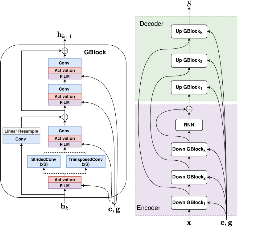
Fig. 1: Generator Schematic. Down GBlocks: downsampling encoder blocks (StridedConv). Up Gblocks: decoder upsampling blocks (TransposedConv). The input x is general to the network. Signals h and (c, g) correspond, respectively, to the input to each GBlock and its conditioning signal’s label and $\sigma$ projections.

The decoder converts the encoder hidden features back to the input signal’s resolution by upsampling with transposed convolutions, employing reversed factors with respect to the encoder. In this case, another stack of GBlocks is inserted. The only difference between these blocks and the ones from the encoder are the change of downsampling stages (linear downsampler in skip connection and strided convolution) by upsampling ones (linear upsampler in skip connection and transposed convolution). Also, each encoder level is connected to its corresponding decoder level through a skip connection. Note that all GBlocks feature 4 convolutional blocks, 4 non-linear activations (LeakyReLUs), and 4 FiLM conditioning layers. To obtain the FiLM conditioning signals, we first process the logarithm of $\sigma$ with random Fourier feature embeddings [3] followed by a multi-layer perceptron (MLP), which yields the embeddings g in Figure 1. Then, g is concatenated with c to drive the FiLM layers.

3 Experimental Setup

3.1 Datasets

To evaluate the effectiveness of DAG to synthesize multiple types of sounds, we resort to two datasets that contain a mixture of impulsive and sustained sound events: UrbanSound8K [23] (US8K) and TUT Acoustic Scenes from DCASE 2016 Task 1 [24] (TUT). US8K contains almost 9 hours of audio, sub-divided into 10 classes that mix ambiance and impulsive sounds, like air conditioner or dog barks. For our experiments, we follow Liu et al. [8] by first partitioning US8K into 8 hours of training data and 50 minutes of test data. Then, we further divide the training split by taking 10% of the files for validation across all folds. TUT contains 13 hours of audio, sub-divided into 15 classes, all of them being mainly ambiance sound. The dataset comes with a pre-made training split of almost 10 hours, with 3 hours of test data. As in US8K, we further divide the training partition by taking 10% of the files for validation.

3.2 Baselines and Configuration

We compare our approach with two state-of-the-art deep generative models for label-based general audio synthesis: the one of Kong et al. [7] (SampleRNN) and the one of Liu et al. [8] (PixelSNAIL). The former operates in the time-domain, hence performing as an end-to-end solution. The latter operates on pre-trained VQ-VAE latent features. As introduced earlier, both are auto-regressive models and, due to their design constraints, they operate at 16 kHz and 22050 Hz, respectively. Here, we re-train both of them at 22050 Hz.

SampleRNN — Following [7], we implement a two-tier conditional SampleRNN with the previously proposed configuration, using the code from the official repository. The model is trained on our data partition using similar hyper-parameters as in the original publication until we observe convergence (300 k and 400 k iterations for US8K and TUT, respectively).

PixelSNAIL — This baseline is based on the three cascaded modules introduced in section 1, which are trained separately: (i) VQ-VAE, (ii) PixelSNAIL, and (iii) HifiGAN [8]. Experiments were conducted using the code from the official repository. The VQ-VAE and PixelSNAIL modules are trained on our data partition with the default hyper-parameters until we observe convergence (100 k and 500 k iterations, respectively), and the HifiGAN module is pre-trained on US8K from the repository. For the results on TUT, we also tried to train the HifiGAN module, but observed worse performance (see section 4.1).

DAG — DAG is built to operate on full-band audio. In this design, which we name DAG48, we choose $\{2,2,4,4,5\}$ as $\Delta_{k}$ stride factors, with block sizes $\{64,128,128,256,512\}$. This way, for 48 kHz waveforms, we obtain latent sequences of 512 dimensions at 150 Hz. Nonetheless, we also make DAG operate on 22050 Hz waveforms (band-limited version) in order to establish a point of comparison with the baselines whilst discarding trivial differences due to bandwidth constraints. We carry out this comparison in two ways. On the one hand, we simply downsample DAG48 generations to 22050 Hz. On the other hand, we adapt the stride factors to make DAG work directly upon 22050 Hz signals, with factors $\{2,2,3,3,5\}$, which approximately correspond to the stride of 7 ms used in full-band. We name this variant DAG22. Both models are trained for 2 M and 1.3 M iterations on US8K and TUT respectively. DAGs are trained via gradient descent with Adam, 8 sequences per batch, and a constant learning rate of $10^{-4}$.

3.3 Objective Metrics

Previous works evaluate their proposals objectively in terms of quality and diversity [7, 8]. Their measures rely on auxiliary classifiers to determine how alike does generated data look with respect to real data, or acoustic features where statistics between sets are compared. More recently, Fréchet audio distance (FAD) was proposed as a metric to assess source separation quality and was shown to better correlate with human judgement when compared to existing metrics. [25]. FAD is built upon a VGGish classifier encoder pre-trained on a source-agnostic dataset. Then, the Fréchet distance between a reference set and an evaluated set is computed on top of the encoder embeddings. Since this metric is proven to be effective in detecting perceptual nuances in the audio [25], it has been recently used to assess audio generation quality [3, 13]. Nevertheless, a potential limitation of using VGGish is in its input features: the model deals with 16 kHz signals, which may suffice for classification but is totally insufficient for full-band synthesis.

In this work, we propose to switch from VGGish to an openly available pre-trained audio encoder that operates upon 48 kHz signals. The motivation is to evaluate the full-band capability of current and future systems performing general audio synthesis. OpenL3 encoders [26] are open source front-ends that operate at 48 kHz (we use the env-mel256 front-end with 512-dimensional embeddings from the official repository). We simply name this metric Fréchet distance (FD), to differentiate it from the previously existing VGGish band-limited approach. Since Fréchet distance variants are known to evaluate both quality and diversity in the generated samples  [27], we also consider a logit score (LS), which follows the Inception score formulation [28] and focuses the analysis on quality itself. This way, a simultaneously low FD and high LS shows a well functioning model in terms of both quality and diversity. LS is computed upon the logit activations of a pre-trained classifier. Departing from the FD feature extractor, we train an MLP per dataset while freezing the OpenL3 front-end. These MLPs are trained until convergence, and the best scoring iterations in validation are selected. They score 83.1 and 97.2% on US8K and TUT test sets, respectively.

4 Results

4.1 Comparison with Existing Approaches

Table 1 shows the FD and LS scores obtained by all models on US8K and TUT. On the one hand, we observe that PixelSNAIL scores better than sampleRNN on US8K, as reported by Liu et al. [8]. On the other hand, we observe that retraining all the modules in the PixelSNAIL cascade for TUT (PixelSNAIL w/ TUT-HifiGAN) leads to an undereperforming model, mainly due to issues with HifiGAN. We hypothesize this may be related to the more environmental nature of TUT, and to the HifiGAN losses not being tuned for this scenario. Nonetheless, since HifiGAN operates as a melspectrogram-to-waveform inverter, we can plug the pre-trained HifiGAN from US8K to do the task in TUT. This makes the model perform competitively again with respect to SampleRNN.

DAG models systematically outperform the baselines and, since the evaluation front-end is pre-trained upon full-band signals, there is a substantial gap between 22050 Hz and 48 kHz models, both in terms of FD and LS. The relative gain of DAG48 upon PixelSNAIL in FD is $58.4\%$ on US8K and $64.9\%$ on TUT. In the band-limited scenario, note that only downsampling DAG48 yields 20.5% and 41% relative gains for FD and LS, respectively, compared to PixelSNAIL in US8K, which was specifically trained to model the band-limited characteristics of the signal alone. In TUT, the FD improvement is 26.6%, and for LS it is 9.4%. However, the DAG22 variant shows that there is room for improving the model performance in band-limited scenarios when training it specifically at 22050 Hz, since the model can score equal or better in FD than DAG48 downsampled. This gap is especially notorious for the TUT dataset. The relative gains for DAG22 upon the baseline then become 24.1% for FD and 40.0% for LS on US8K. For TUT, the relative gains are 39.6% and 18.9% over PixelSNAIL.

Model	Samp. rate	Num. param.		US8K			TUT
				FD  $\downarrow$	LS  $\uparrow$		FD  $\downarrow$	LS  $\uparrow$
SampleRNN [7]	22 kHz	41 M		237.0	2.80		138.8	2.07
PixelSNAIL [8]	22 kHz	119 M		115.1	3.27		107.3	4.65
PixelSNAIL [8] w/ TUT-HifiGAN	22 kHz	119 M		n/a	n/a		144.3	3.33
DAG48 + Downsample	22 kHz	22 M		91.4	5.54		78.8	5.13
DAG22	22 kHz	22 M		87.4	5.45		64.8	5.74
DAG48	48 kHz	22 M		47.9	6.21		37.7	6.59
Real data	22 kHz	-		72.6	5.26		79.0	5.53
Real data (test set)	48 kHz	-		30.9	6.33		3.7	9.31

Table 1: Fréchet distance (FD) and logit score (LS) results on US8K and TUT data sets. DAG models were generated with sampling parameters $\alpha=2$, $N=100$, $\gamma=2$ for US8K, and $\gamma=0$ for TUT. Metrics computed with OpenL3 at 48 kHz.

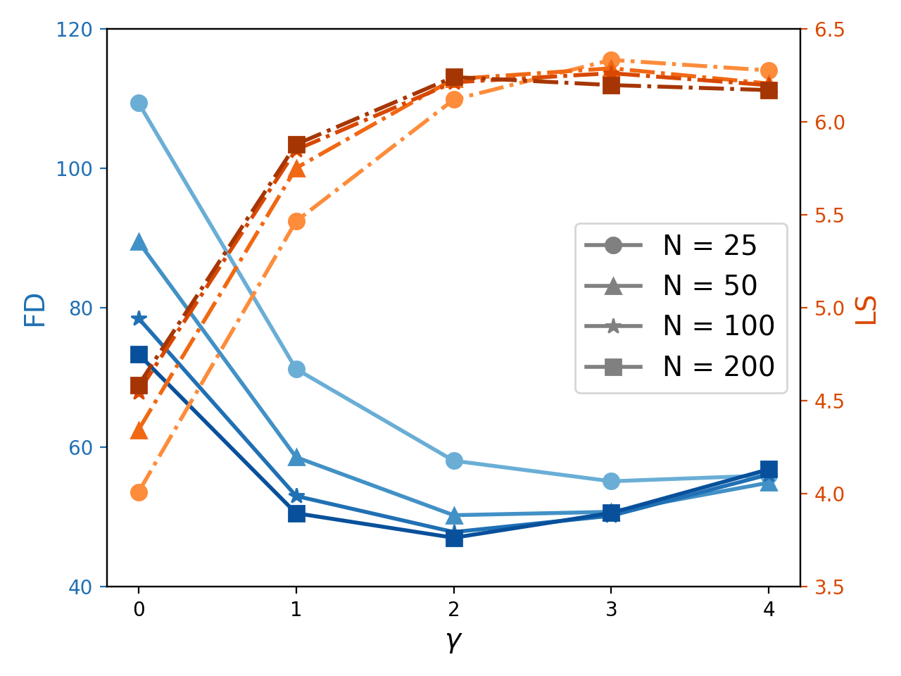
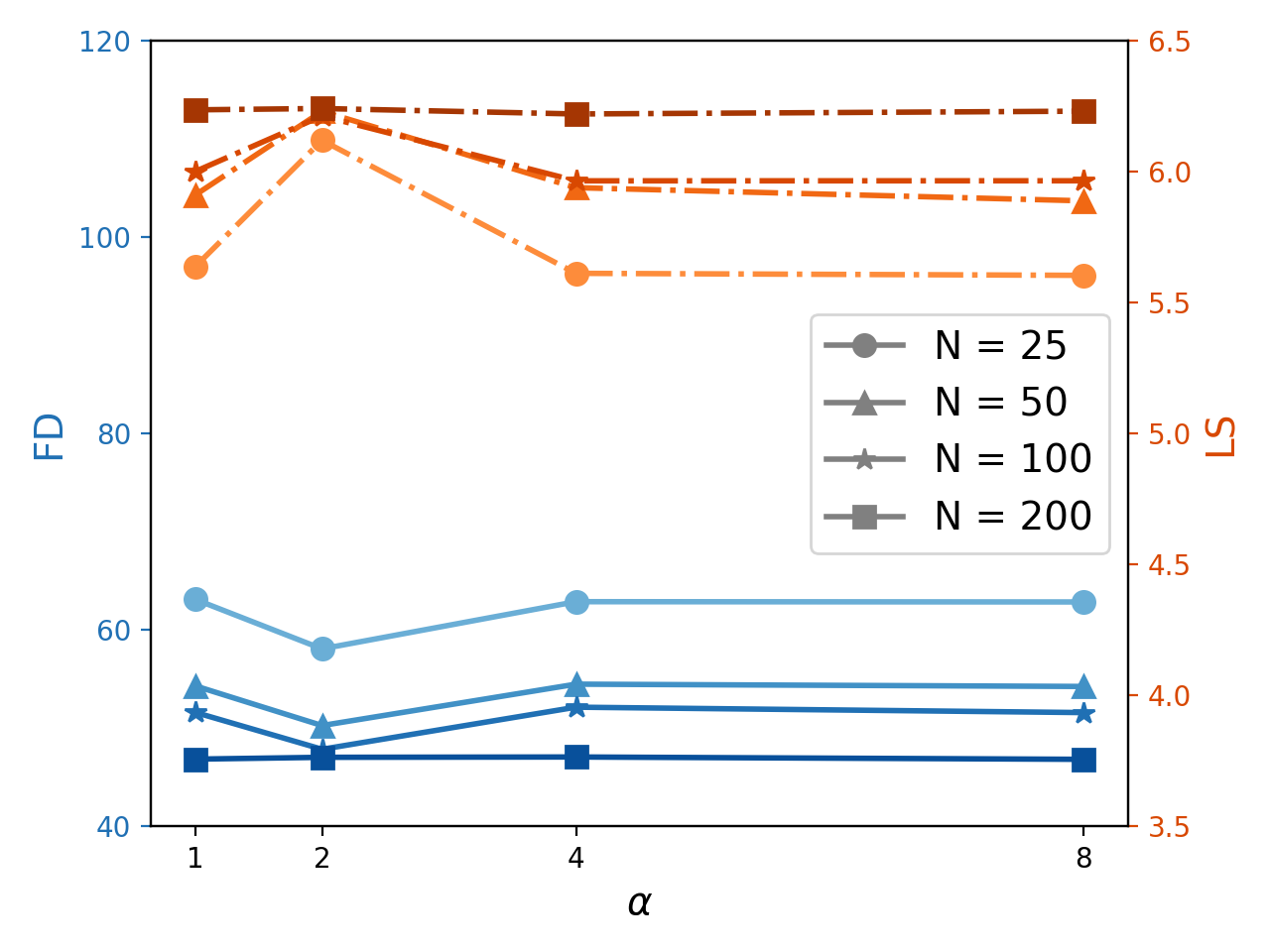
Fig. 2: DAG48 performance as a function of the classifier-free guidance weight $\gamma$ using $\alpha=2$ (left) and the sampling hyper-parameter $\alpha$ using $\gamma=2$ (right) for different number of sampling steps $N$: Fréchet distance (FD) and logit score (LS) on US8K dataset. Metrics computed with OpenL3 at 48 kHz.

4.2 Effect of Guidance and Sampling Hyper-parameters

Figure 2 shows DAG48 performance when changing the classifier-free guidance weight $\gamma$ (left), as well as the sampling hyper-parameter $\alpha$ (right). Regarding $\gamma$, its increase translates into a quick improvement of the synthesis quality, especially with a low amount of steps in the Langevin sampling $N$. This means that a model with $50$ steps can already get a competitive performance with $\gamma=2$, which reduces substantially the computational cost when compared to $N=200$. Note that when $N$ is increased, a higher guidance weight degrades the quality, and that this degradation is faster with longer sampling processes. The fact that the LS curves saturate with $\gamma=4$ but FD increases may indicate a loss in diversity at the expense of more realism, something intrinsic to the classifier-free guidance technique [21]. Regarding $\alpha$, we observe a trend where the choice of a particular value seems to be less critical, especially if we can afford to sample with $N=200$ steps. Nevertheless, a factor $\alpha=2$ works well overall, and is of importance when we want to reduce the sampling computational complexity with $N<200$.

4.3 Additional Samples and Qualitative Analysis

It is observed that the TUT and US8K datasets contain mostly noisy ambiance with some target sound events happening in the background, which makes it difficult to identify if some low-quality synthesis samples are due to the training data or a model limitation. Therefore, we use additional clean foreground sounds as training data to further experiment with DAG’s modeling capability and generation quality. This data is an in-house collection of carefully-picked high-quality samples from Freesound, including wind, rain, river, waves, fire, footsteps, applause, horses, and piano music. This selection aims at covering a wider range of signal characteristics, from modulated noise and sinusoids to transients.

The resulting synthesis samples are promising: the attacks of footsteps, fire crackling or piano sound crispy; the noisy wind, rain, or waves sound naturally smooth; the individual bubbling in river and the individual clapping in crowd applause can be heard clearly. Some generated examples are available for listening on the project website as a demonstration of DAG’s great potential to synthesize general audio with quality and diversity. Moreover, we show some results of a simple audio style transfer approach enabled by DAG’s modeling strategy. Here, we inject a normalized input signal y before the first sampling step, such that $\textbf{x}_{1}=\textbf{y}+\sigma_{1}\textbf{z}_{1}$ (see equation 1).

5 Conclusions

In this work, we propose the diffusion audio generator, a full-band general audio synthesis model based on score-based diffusion. With this, we tackle the source-agnostic audio synthesis problem with an end-to-end solution capable of outperforming the state of the art in a label-to-audio setup for two datasets that mix environmental and impulsive sounds. Moreover, we investigate the effectiveness of recent sampling techniques for diffusion models, like classifier-free guidance, showing that it can greatly benefit the performance of our model whilst reducing the amount of sampling steps needed to achieve a certain level of quality.

6 Acknowledgements

We would like to thank Giulio Cengarle for fruitful guidance on signal processing methods.

References

- [1] Paul Taylor, Text-to-speech synthesis, Cambridge university press, 2009.
- [2] Prafulla Dhariwal, Heewoo Jun, Christine Payne, Jong Wook Kim, Alec Radford, and Ilya Sutskever, “Jukebox: A generative model for music,” ArXiv: 2005.00341, 2020.
- [3] Simon Rouard and Gaëtan Hadjeres, “CRASH: Raw audio score-based generative modeling for controllable high-resolution drum sound synthesis,” in Proc. of the Int. Soc. for Music Information Retrieval Conf. (ISMIR), 2021, pp. 579–585.
- [4] Javier Nistal, Stefan Lattner, and Gael Richard, “DrumGAN: Synthesis of drum sounds with timbral feature conditioning using generative adversarial networks,” in Proc. of the Int. Soc. for Music Information Retrieval Conf. (ISMIR), 2020, pp. 490–498.
- [5] Marco Comunità, Huy Phan, and Joshua D Reiss, “Neural synthesis of footsteps sound effects with generative adversarial networks,” in Conv. of the Audio Eng. Soc. (AES), 2021, p. 10583.
- [6] M Mehdi Afsar, Eric Park, Étienne Paquette, Gauthier Gidel, Kory W Mathewson, and Eilif Muller, “Generating diverse realistic laughter for interactive art,” NeurIPS Workshop on Machine Learning for Creativity and Design (ML4CD), 2021.
- [7] Qiuqiang Kong, Yong Xu, Turab Iqbal, Yin Cao, Wenwu Wang, and Mark D Plumbley, “Acoustic scene generation with conditional SampleRNN,” in Proc. of the IEEE Int. Conf. on Acoustics, Speech and Signal Processing (ICASSP), 2019, pp. 925–929.
- [8] Xubo Liu, Turab Iqbal, Jinzheng Zhao, Qiushi Huang, Mark D Plumbley, and Wenwu Wang, “Conditional sound generation using neural discrete time-frequency representation learning,” in IEEE Int. Workshop on Machine Learning for Signal Processing (MLSP), 2021, pp. 1–6.
- [9] Ali Razavi, Aaron Van den Oord, and Oriol Vinyals, “Generating diverse high-fidelity images with VQ-VAE-2,” Advances in Neural Information Processing Systems (NeurIPS), vol. 32, pp. 14866–14876, 2019.
- [10] Xi Chen, Nikhil Mishra, Mostafa Rohaninejad, and Pieter Abbeel, “PixelSNAIL: An improved autoregressive generative model,” in Proc. of the Int. Conf. on Machine Learning (ICML). PMLR, 2018, pp. 864–872.
- [11] Jungil Kong, Jaehyeon Kim, and Jaekyoung Bae, “Hifi-GAN: Generative adversarial networks for efficient and high fidelity speech synthesis,” Advances in Neural Information Processing Systems (NeurIPS), vol. 33, pp. 17022–17033, 2020.
- [12] Dongchao Yang, Jianwei Yu, Helin Wang, Wen Wang, Chao Weng, Yuexian Zou, and Dong Yu, “DiffSound: Discrete diffusion model for text-to-sound generation,” ArXiv: 2207.09983, 2022.
- [13] Felix Kreuk, Gabriel Synnaeve, Adam Polyak, Uriel Singer, Alexandre Défossez, Jade Copet, Devi Parikh, Yaniv Taigman, and Yossi Adi, “AudioGen: Textually guided audio generation,” ArXiv: 2209.15352, 2022.
- [14] Yang Song and Stefano Ermon, “Generative modeling by estimating gradients of the data distribution,” in Advances in Neural Information Processing Systems (NeurIPS), vol. 32, pp. 11895–11907. 2019.
- [15] Yang Song, Jascha Sohl-Dickstein, Diederik P. Kingma, Abhishek Kumar, Stefano Ermon, and Ben Poole, “Score-based generative modeling through stochastic differential equations,” in Proc. of the Int. Conf. on Learning Representations (ICLR), 2021.
- [16] Zhifeng Kong, Wei Ping, Jiaji Huang, Kexin Zhao, and Bryan Catanzaro, “DiffWave: A versatile diffusion model for audio synthesis,” in Proc. of the Int. Conf. on Learning Representations (ICLR), 2020.
- [17] Nanxin Chen, Yu Zhang, Heiga Zen, Ron J Weiss, Mohammad Norouzi, and William Chan, “WaveGrad: Estimating gradients for waveform generation,” in Proc. of the Int. Conf. on Learning Representations (ICLR), 2020.
- [18] Joan Serrà, Santiago Pascual, Jordi Pons, R Oguz Araz, and Davide Scaini, “Universal speech enhancement with score-based diffusion,” ArXiv: 2206.03065, 2022.
- [19] Alexia Jolicoeur-Martineau, Rémi Piché-Taillefer, Rémi Tachet des Combes, and Ioannis Mitliagkas, “Adversarial score matching and improved sampling for image generation,” in Proc. of the Int. Conf. on Learning Representations (ICLR), 2021.
- [20] Joan Serrà, Santiago Pascual, and Jordi Pons, “On tuning consistent annealed sampling for denoising score matching,” ArXiv: 2104.03725, 2021.
- [21] Jonathan Ho and Tim Salimans, “Classifier-free diffusion guidance,” ArXiv: 2207.12598, 2022.
- [22] Chitwan Saharia, William Chan, Saurabh Saxena, Lala Li, Jay Whang, Emily Denton, Seyed Kamyar Seyed Ghasemipour, Burcu Karagol Ayan, S. Sara Mahdavi, Rapha Gontijo Lopes, Tim Salimans, Jonathan Ho, David J. Fleet, and Mohammad Norouzi, “Photorealistic text-to-image diffusion models with deep language understanding,” ArXiv: 2205.11487, 2022.
- [23] Justin Salamon, Christopher Jacoby, and Juan Pablo Bello, “A dataset and taxonomy for urban sound research,” in Proc. of the ACM Int. Conf. on Multimedia (ACM-MM), 2014, pp. 1041–1044.
- [24] Annamaria Mesaros, Toni Heittola, and Tuomas Virtanen, “TUT database for acoustic scene classification and sound event detection,” in Proc. European Signal Processing Conference (EUSIPCO), 2016, pp. 1128–1132.
- [25] Kevin Kilgour, Mauricio Zuluaga, Dominik Roblek, and Matthew Sharifi, “Fréchet audio distance: A reference-free metric for evaluating music enhancement algorithms.,” in Proc. of the Conf. of the Int. Speech Communication Association (INTERSPEECH), 2019, pp. 2350–2354.
- [26] Jason Cramer, Ho-Hsiang Wu, Justin Salamon, and Juan Pablo Bello, “Look, listen, and learn more: Design choices for deep audio embeddings,” in Proc. of the IEEE Int. Conf. on Acoustics, Speech and Signal Processing (ICASSP), 2019, pp. 3852–3856.
- [27] Muhammad Ferjad Naeem, Seong Joon Oh, Youngjung Uh, Yunjey Choi, and Jaejun Yoo, “Reliable fidelity and diversity metrics for generative models,” in International Conference on Machine Learning. PMLR, 2020, pp. 7176–7185.
- [28] Shane Barratt and Rishi Sharma, “A note on the inception score,” ArXiv: 1801.01973, 2018.