Multi-Objective Hardware-Mapping Co-Optimisation
for Multi-Tenant DNN Accelerators

Abstract

To meet the ever-increasing computation demand from emerging workloads, a scalable design paradigm combines multiple Deep Neural Network (DNN) accelerators to build a large multi-accelerator system. They are mainly proposed for data centers, where workload varies across vision, language, recommendation, etc. Existing works independently explore their hardware configuration and mapping strategies due to the extremely large cross-coupled design space. However, hardware and mapping are interdependent and, if not explored together, may lead to sub-optimal performance when workload changes. Moreover, even though a data center accelerator has multiple objectives, almost all the existing works prefer aggregating them into one (mono-objective). But aggregation does not help if the objectives are conflicting, as improving one will worsen the other.

This work proposes MOHaM, a multi-objective hardware-mapping co-optimisation framework for multi-tenant DNN accelerators. Specifically, given an application model and a library of heterogeneous, parameterised and reconfigurable sub-accelerator templates, MOHaM returns a Pareto-optimal set of multi-accelerator systems with an optimal schedule for each one of them to minimise the overall system latency, energy and area. MOHaM is evaluated for diverse workload scenarios with state-of-the-art sub-accelerators. The Pareto-optimal set of competitive design choices enables selecting the best one as per the requirement.

I Introduction

Deep Neural Network (DNN) accelerators drives the era of Domain-Specific Architectures (DSAs). From edge [2] to the cloud [5], they are ubiquitous to enable performance improvement for different workloads. To meet the ever-increasing computation demand from emerging workloads, a scalable design paradigm combines multiple sub-accelerators to build a large accelerator system. Existing works have explored the combination of both, homogeneous as well as heterogeneous sub-accelerators [50][5][4][8][12][18][33][35][28]. Conceptual view of a multi-accelerator system is shown in Figure 1.

Due to limited area and power budget at the edge, multi-accelerator systems are usually employed in the cloud, i.e., data centers. Two of the most important factors deciding a DNN accelerator performance are its hardware configuration and mapping strategy. Their design spaces are extremely large and hence are often explored independently [24][23][53][26]. With multiple sub-accelerators, these design spaces are only becoming larger in multi-accelerator systems. For example, MAGMA [28] reported the design space of mapping alone to be of size $O(1e81)$. However, hardware and mapping are interdependent and, if not explored together, may lead to sub-optimal performance when workload changes [32]. As multi-accelerator systems are proposed for data centers, where workload varies across vision, language, recommendation, etc., each with different variants of DNNs [7][41], hardware-mapping co-optimisation is very important and timely. Some works on co-optimisation are available [29][48][55][57], but they do not discuss multi-accelerator systems due to the obvious challenge of huge cross-coupled search space. Table 1 presents the existing works on multi-accelerator systems, where Planaria [18] and Herald [33] are the only ones attempting co-optimisation. Nevertheless, Planaria lacks dataflow flexibility, and both of them rely on heuristic-based (manually-designed) decision-making. This limits their scalability towards diverse sub-accelerators and emerging workloads.

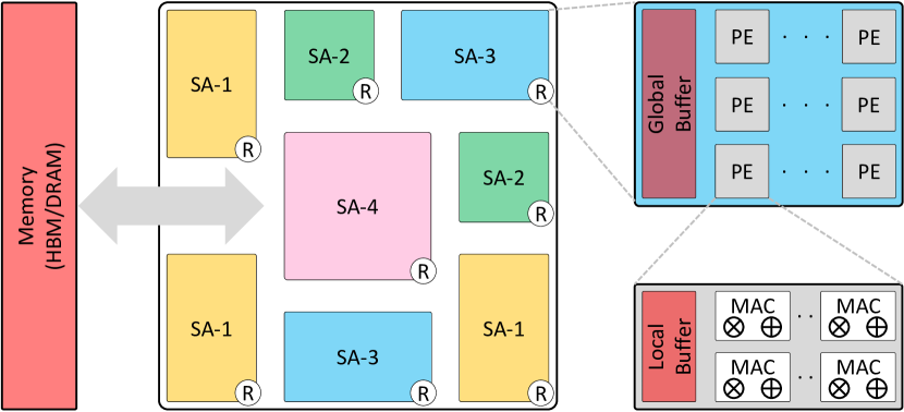
Figure 1: A DNN multi-accelerator system.

A primary enabler of scalability in data centers is multi-tenancy, where different DNN models are simultaneously executed on an accelerator. Multi-tenancy trivially becomes a key aspect in multi-accelerator systems as they house sub-accelerators supporting diverse DNNs. As given in Table 1, quite a few existing works have support for multi-tenancy. However, except MAGMA [28], which uses Genetic Algorithm (GA), all employed manually-designed support, which may limit accelerator utilisation and deployment benefits.

Designing an accelerator for data center often has more than one objective, like a subset of latency (delay), throughput, energy, area, temperature, etc. A convenient way of exploration preferred in the existing works is the aggregation of multiple objectives into one (mono-objective), say, Energy-Delay-Product (EDP). However, a chosen group of objectives might be conflicting with one another; in which case, aggregation does not help. Hence, a multi-objective exploration is necessary for identifying multiple design points to select the most suitable one according to the requirement. MEDEA [48] is the only work focusing on true multi-objective exploration of DNN accelerators. As given in Table 1, none of the existing multi-accelerator systems have explored in this direction.

This work proposes a Multi-Objective Hardware-Mapping co-optimisation framework (MOHaM) for multi-tenant DNN accelerators . It is the first attempt at simultaneous exploration of hardware configuration and mapping strategy for multi-tenancy with multiple distinct objectives. Specifically, the proposed work makes the following major contributions:

Table 1: Comparison of existing works on multi-accelerator systems based on design space exploration of hardware, mapping, multi-tenency (Mul-Ten) and multi-objective (Mul-Obj).

Work	Hardware	Mapping	Mul-Ten	Mul-Obj
Simba [50]
TPUv4 [5]
CS-2 [4]
AI-MT [8]
PREMA [12]
Planaria [18]
Herald [33]
VELTAIR [35]
MAGMA [28]
MOHaM

1. Given an application model and a library of heterogeneous, parameterised and reconfigurable sub-accelerator templates, MOHaM returns a Pareto-optimal set of multi-accelerator systems with an optimal schedule for each one of them to minimise latency, energy and area.

2. To search the enormous design space, MOHaM extends the NGSA-II [14] multi-objective GA with several custom genetic operators specific to the problem definition. This improves the search efficiency and makes MOHaM much faster than the standard optimisation techniques.

3. Experimental evaluation with diverse workload scenarios and state-of-the-art sub-accelerators show that MOHaM is able to generate competitive design points considering all the objectives. To the best of the author’s knowledge, this is the first work offering hardware-mapping co-optimisation, support for multi-tenancy and multi-objective exploration, all in a single framework.

II Background

II-A Multi-Accelerator System

As shown in Figure 1, it is a coming together of multiple DNN accelerators (called sub-accelerators in the bigger context). To ensure scalability, this work considers a Multi-Chip-Module (MCM) based multi-accelerator system, like Simba [50], where each of the Sub-Accelerators (SAs) is a chiplet connected by a Network-on-Package (NoP). However, unlike Simba, which combines homogeneous chiplets, the multi-accelerator system in this work considers heterogeneity to support diverse DNN models and emerging workloads.

II-A1 Sub-Accelerator Architecture

Each SA is a standard DNN accelerator with an array of Processing Elements (PEs) and a shared Global Buffer (GB) [9]. Each PE houses one or more Multiply-Accumulate (MAC) units to compute partial sums and a Local Buffer (LB) to store them. GB collects weights and activations from the memory (HBM/DRAM) through the NoP and distributes them to the LBs through the Network-on-Chip (NoC). Similarly, outputs are written from LB to GB and then to memory through NoC and NoP, respectively. Existing literature has many promising DNN accelerators that could be used as an SA chiplet to build a multi-accelerator system [43][50][10][3][6][40][20][15].

II-A2 DNN Models

Data center workloads mainly revolve around vision, language and recommendation-based DNN models [7][46][41]. Based on the shape and operation, different layers of a DNN model may have a specific dataflow preference. However, most of the SAs are usually optimised for some specific layers with a fixed dataflow [33]. Figure 2(a) shows how the normalised EDP varies when the same DNN model is run on different SAs. Here, three dominant layers, Convolution CONV_0 and CONV_33, and Fully Connected FC_121 from the ResNet50 DNN model [21] are considered. These layers are individually run on row-stationary (Eyeriss [9]), weight-stationary (Simba [50]) and output-stationary (ShiDianNao [15]) SAs. Similar observations are available in the literature [33][57][39][32][34] but the objective here is to advocate for flexible accelerators. A multi-accelerator system for data centers should consider heterogeneous SAs for dataflow flexibility to diverse and emerging DNN models.

II-B Hardware-Mapping Co-Optimisation

A typical hardware-mapping co-optimisation framework takes as input, a target DNN model, an optimisation objective (e.g. latency) and the resource constraints (e.g. area). It returns as output a hardware configuration with the optimal instances of resources and an optimal mapping strategy to run the DNN model on the accelerator. This co-optimisation can be used at design-time to build a more efficient accelerator. However, the search space is extremely large as it is the cross-product of hardware and mapping. For example, DiGamma [29] recently reported a design space as large as $O(10^{36})$, and that is only for a single accelerator. The same space for a multi-accelerator system could reach up to $O(10^{55})$ with just 4 ResNet50-like DNN models and 16 SAs, by using equation (1) through (5).

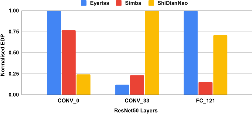
(a)

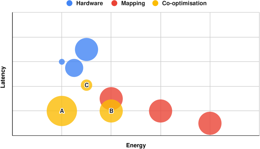
(b)

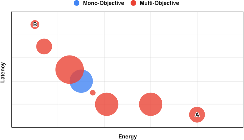
(c)

Figure 2: Need for heterogeneity, co-optimisation and multi-objective exploration.

III Motivation

Figure 2(b) and 2(c) shows a conceptual representation of the design space exploration with three optimisation objectives, energy (x-axis), latency (y-axis) and area (size of the design points). Figure 2(b) shows design points with hardware-only optimisation (blue), mapping-only optimisation (red), and co-optimisation (yellow). The blue design points, in general, have lower energy and area as a result of optimal hardware resources but relatively higher latency due to fixed mapping strategy. On the contrary, the red design points have lower latency as a result of optimal mapping strategy but a fixed area (all are of the same size!) due to fixed hardware configuration. The yellow design points do not follow a fixed pattern and provide some interesting options. For example, with a small increase in area than the mapping-only optimisation, design point A has much lower energy and latency. The increased area due to additional hardware resources allows a better mapping strategy (co-optimisation). Design point B shows that an area slightly lower than A has no impact on latency but increases energy. Design point C shows that a small compromise on latency can significantly improve energy as well as area. In this way, co-optimisation may offer competitive design points.

The conventional way of aggregating multiple optimisation objectives into one (mono-objective) is shown in blue in Figure 2(c). This practice offers a single design point which might not be optimal if objectives conflict. For example, due to the chosen memory hierarchy, if the system bandwidth is insufficient to feed enough data into the compute (MAC) units, they remain underutilised. In such a scenario, two mapping strategies may output identical latency but varying hardware resource utilisation, hence different energy and area. Similarly, it is possible to either access an enlarged on-chip buffer or the next-level buffer (memory) within the same energy budget. In such a scenario, even two hardware-mapping co-optimisations may output identical energy but different latency and area. These scenarios can be expressed as a set of non-dominating design points (multi-objective), as shown in red in Figure 2(c). These Pareto-optimal set of distinct multi-objective solutions allow simultaneously exploring accelerator designs with varying requirements. To give a specific use case, suppose the accelerator needs to be deployed for remote robotic surgery with hard real-time constraints. Then design point A with the lowest latency is preferred without bothering about energy and area. In another use case, energy and area are paramount when the accelerator is deployed for consumer wearables like smart glasses. Design point B could be the preferred choice then. These factors motivated the MOHaM framework to target multi-objective co-optimisation in multi-accelerator systems.

IV Problem Formulation

This section first defines the inputs and outputs of the proposed MOHaM framework, then formulates the exploration problem and finally computes the size of the search space. Most of the acronyms/abbreviations and terms used to explain the MOHaM framework are presented in Table 2 for reference.

IV-A Definitions

Definition 1.

A DNN model is a directed graph $DNN=G(L,D)$ where $L$ is the set of layers and $D$ is the set of dependencies between layers. For example, a layer dependency $d=(l_{i},l_{j})\in D,\ l_{i},l_{j}\in L$ states that layer $l_{j}$ can be executed only after layer $l_{i}$. A layer $l\in L$ has a set of properties like, the type of layer (e.g., CONV_0, FC_121), the shape of input activation and weights (e.g., width, height, channels), etc.

Definition 2.

An Application Model, $AM(L,D)$, is a set of DNN models $\{DNN_{i}(L_{i},D_{i})\}$ where $L=\cup_{i}L_{i}$ and $D=\cup_{i}D_{i}$. The DNN models within an $AM$ are assumed to be independent of each other and thus can be executed in parallel.

For example, $AM$ for an Augmented Reality (AR) application will have multiple DNN models, each with a specific task like object detection, gesture identification, depth estimation, etc. Figure 3(a) shows an $AM$ formed by three $DNN$ models.

Definition 3.

A Sub-Accelerator Template, $SAT$, is a parameterised and reconfigurable DNN accelerator supporting different hardware configurations as well as mapping strategies.

For example, a modifiable Simba chiplet [50] could be a $SAT$.

Definition 4.

A Sub-Accelerator Instance, $SAI$, is an instance of a $SAT$ configured with specific values to its parameters.

For example, Simba $SAT$ becomes a Simba $SAI$ when its configurable parameters are given values, like, 128 PEs, 256 KiB GB, 32 KiB LB, weight-stationary dataflow, etc.

Definition 5.

A Network-on-Package (NoP) is a directed graph $NoP=G(T,C)$ where $T$ is the set of tiles and $C$ is the set of communication links. A tile $t\in T$ hosts a $SAI$ and has a router to communicate with other tiles in the package.

Definition 6.

A Multi-Accelerator System, $MAS$, is a tuple $\langle SSAI,NoP,SMI,PF\rangle$ where $SSAI$ is the set of heterogeneous $SAI$ chiplets and $SMI$ is the set of Memory Interfaces ($MI$s) for external HBMs/DRAMs, all connected together by the $NoP$. $PF$ is the placement function such that for a $SAI\in SSAI$ or a $MI\in SMI$, it returns the hosting tile.

Figure 3(d) shows a $MAS$ created by eight $SAI$s and an external memory, interconnected by an $NoP$. The $SAI$s are instances of four parameterised and reconfigurable $SAT$s, as shown in Figure 3(b). For example, $SAI0.0$, $SAI0.1$ and $SAI0.2$ are three different instances of $SAT0$ and so on.

Definition 7.

A Schedule, $S(MAS,AM)$, for an $AM(L,D)$ is a directed bipartite graph $S=G(L,SSAI,D^{+},M)$ where $D^{+}\supseteq D$ is the set of edges that models the dependencies among layers at the application level. $M$ is the set of edges that maps a layer $l\in L$ into a chiplet $SAI\in SSAI$.

For example, Figure 3(e) shows a schedule for the $AM$ in Figure 3(a) and the $MAS$ in Figure 3(d). $D^{+}$ and $M$ are shown by black and red edges, respectively. $D^{+}$ might contain dependencies like $d^{\prime}$ and $d^{\prime\prime}$ that are not present in $D$. Both, $L0.3$ of $DNN0$ and $L2.2$ of $DNN2$ are mapped onto $SAI3.0$. $d^{\prime}$ defines the execution order and dictates that $L0.3$ be run only after $L2.2$. Similarly, $d^{\prime\prime}$ dictates $L0.3$ be run first.

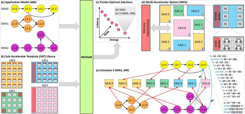
Figure 3: Working of the MOHaM framework.

IV-B Problem Formulation

Given an application model, $AM$, and a library of heterogeneous, parameterised and reconfigurable sub-accelerator templates, $SAT$s, find the Pareto-optimal set of multi-accelerator systems, $MAS$, and an optimal schedule, $S$, for each one of them to minimise the overall system latency, energy and area.

IV-C Search Space

Search for the Pareto-optimal set of solutions involves a design space exploration that is an $n$-fold Cartesian product of SA hardware space, SA mapping space, layer-to-SA mapping space, SA-to-tile mapping space, and schedule space.

Major SA hardware includes PEs, MACs, GB, LB, etc. For each $SAT$, let $np$ be the number of free parameters and $v$ be the number of configurable values a free parameter can have. Then for the entire $SSAI$, the size of SA hardware space is:

$$v^{np}\times\left|SSAI\right|$$ (1)

DNN models are represented by tensors, and their computation involves multiple loops. A dataflow defines the loop order, parallelism and clustering, and is usually expressed in a loop-nest form [9][57][33][29]. Mapping determines tiling, i.e. how tensors are sliced, stored and transferred across the memory hierarchy, and uses a dataflow to map a layer $l$ into an $SAI$. Let $nl$ be the depth of loop-nest, $C$ and $K$ be the input and output channels, $Y$ and $X$ be the width and height of input activation, and $R$ and $S$ be the width and height of weights. For $AM(L,D)$, the size of SA mapping space is:

$$nl!\times 2^{nl}\times(C\times K\times Y\times X\times R\times S)\times\left|L\right|$$ (2)

where, $nl!$ is the loop order, $2^{nl}$ is for parallelism and clustering, and $(C\times K\times Y\times X\times R\times S)$ is for the tiling.

As each layer of the $AM(L,D)$ can be mapped onto each of the $SAI$s, the size of layer-to-SA mapping space is:

$$\left|L\right|\times\left|SSAI\right|$$ (3)

Each $SAI$ can be mapped onto a tile $t$ of the $NoP$. Let the number of tiles corresponds to the number of SA instances (i.e., $\left|T\right|\equiv\left|SSAI\right|$). Then the size of SA-to-tile mapping space is the permutation of SAs in different tiles, which is:

$$\left|SSAI\right|!$$ (4)

Finally, let each DNN model of an $AM(L,D)$ has $l$ layers, and none are parallel. If the $AM(L,D)$ is formed by $nd$ parallel DNN models, the size of the schedule space is:

$$(nd!\times l)\times l^{nd}$$ (5)

The complete search space is the product of equation (1) through (5), and changes factorially with the number of DNN models, SAs and the depth of loop-nest in the $AM(L,D)$.

V The MOHaM Framework

Table 2: Acronyms/abbreviations and terms used for MOHaM

AM	Application Model; a set of independent DNN models.
SAT	Sub-Accelerator Template; a parameterised and reconfigurable DNN accelerator with a fixed memory hierarchy.
SAI	Sub-Accelerator Instance of a SAT with fixed parameters.
MAS	Multi-Accelerator System; a set of SAIs.
S	Schedule; temporal and spatial allocation of all the DNN model layers of an AM on the SAIs of a MAS.
NSGA-II	Non-Dominated Sorting Genetic Algorithm [14].
Gene	A tuple of encoded values for a layer or an SA instance.
Genome	An array of genes that represent either all the information about layers or SAIs, like mapping, execution order, etc.
Chromosome	A concatenation of genomes of all the layers and SAIs.
Individual	A chromosome with valid mapping, SAI and execution order of the layers, and SAT and NoP tiles for the SAIs.
Population	A set of individuals evolving through GA generations.
Pareto Efficiency	An individual is Pareto-efficient if no one else in the population is better for all the objectives at the same time.
Topological Sort	A linear ordering of a Directed Acyclic Graph (DAG) where a node appears before all the nodes it points to.

Algorithm 1 MOHaM High-Level Flow

procedure LayerMapper($AM,SSAT$)

     $MG\leftarrow\{\}$

     for $layer$ in UniqueLayers($AM$) do

         $ML\leftarrow\{\}$

         for $arch$ in $SSAT$ do

              $MF\leftarrow\textsc{RunMedea}(layer,arch)$

              $ML$.Add($MF$)

         end for

         $MG$.Add($ML$)

     end for

     return $MG$

end procedure

procedure GlobalScheduler($AM,SSAT,MG$)

     $PP\leftarrow\textsc{InitialPopulation}()$

     for $g\leftarrow 1$ to $G$ do $\triangleright$ G is the number of generations

         $OP\leftarrow\textsc{ApplyCrossoverOperators}(PP)$

         $OP$.$\textsc{ApplyMutationOperators}(OP)$

         $OP$.$\textsc{Evaluate}()$

         $MP\leftarrow\textsc{FastNonDominatedSorting}(PP,OP)$

         $OP\leftarrow\textsc{Survival}(MP)$

     end for

     return $PP$.$\textsc{GetParetoEfficientIndividuals}()$

end procedure

procedure MOHaM($AM,SSAT$)

     $MG\leftarrow\textsc{LayerMapper}(AM,SSAT)$

     $ST\leftarrow\textsc{GlobalScheduler}(AM,SSAT,MG)$

     return $ST$ $\triangleright$ Return Pareto Set of Schedulings

end procedure

To search the enormous design space, the proposed MOHaM framework adopts a two-step approach, layer mapping and global scheduling. In the first step, each layer of the $AM(L,D)$ is mapped onto each of the $SAT$s available in the input library. Then the Pareto-optimal set of mappings found for each layer is used in the second step to search the global scheduling. MOHaM is written in C++ and uses the Timeloop [39] + Accelergy [54] framework for realising both the steps. Algorithm 1 presents a high-level flow of MOHaM, and the following sub-sections describe its working in detail.

V-A Layer Mapper

Let $SSAT$ be the set of $SAT$s available in the input library. As per equation (3), if each layer of the $AM(L,D)$ is mapped onto each of the $SAT$s, the search space can be as large as $\left|L\right|\times\left|SSAT\right|$. However, two layers, $\ l_{i},l_{j}\in L$ can be instances of the same workload, i.e., have the same problem dimensions. Hence, in an attempt to reduce the layer mapping search space, MOHaM only maps the unique layers to each of the $SAT$s.

Let $M_{l,f,i}$ be a mapping for a layer $l\in L$ in an SA template $f\in SSAT$. $M_{l,f,i}$ is a choice of a specific tiling, loop ordering, paralellism and clustering in $f$. Now, let $MF_{l,f}$ be the Pareto-optimal set of mappings with respect to latency, energy and area for $l$ in $f$. $MF_{l,f}$ can be represented by:

$$MF_{l,f}=\{\,M_{l,f,i}\mid i=0,\dots,(m_{l,f}-1)\,\}$$ (6)

where, $m_{l,f}$ is the number of Pareto-optimal mappings. Now, let $ML_{l}$ be the Pareto-optimal set of mappings for $l$ in all the input SA templates of $SSAT$. $ML_{l}$ can be represented by:

$$ML_{l}=\{\,MF_{l,f}\mid f=0,\dots,(F-1)\,\}$$ (7)

where, $F$ is the number of input SA templates, i.e., $\left|SSAT\right|$. Finally, let $MG$ be the Pareto-optimal set of mappings for all the layers of $AM(L,D)$ in all the input SA templates of $SSAT$. $MG$ can be represented by:

$$MG=\{\,ML_{l}\mid l=0,\dots,(L-1)\,\}$$ (8)

where, L is the number of layers in the $AM(L,D)$. To obtain the Pareto-optimal sets in equation (6) through (8), MOHaM leverage state-of-the-art MEDEA [48] infrastructure. For the optimisation objectives, latency, energy and area, MEDEA searches for a Pareto-optimal set of mappings for a layer on a $SAI$ employing a GA with custom operators. MEDEA can only map a single layer on a single accelerator, while MOHaM has the capability for multi-DNN models and multi-accelerator systems. MOHaM decides $SAI$s, their hardware parameters, and schedule layers with appropriate mappings and $SAI$s. Hence, as given in Algorithm 1, MEDEA is just one component of MOHaM’s complex multi-objective search.

V-B Global Scheduler

It is based on one of the most widely accepted multi-objective GA, NGSA-II [14]. It has five major phases, sampling, selection, crossover, mutation and survival. The scheduler uses the original selection and survival phases of the NGSA-II. However, multiple custom genetic operators are implemented for problem-specific crossover and mutation, and also for increasing the sampling efficiency to find better individuals in less time. The global scheduler of MOHaM returns a Pareto-optimal set of $MAS$ and an optimal $S$ for each one of them with minimum latency, energy and area.

V-B1 Chromosome Encoding

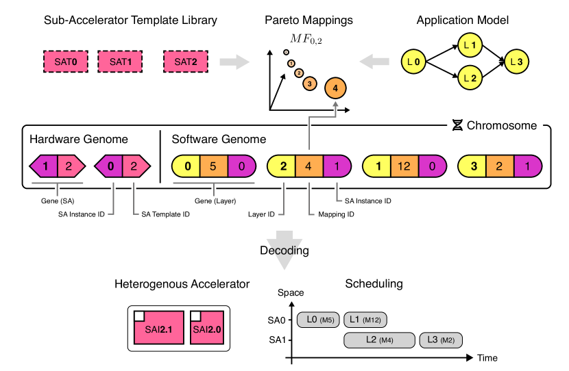
Figure 4: MOHaM global scheduler chromosome structure.

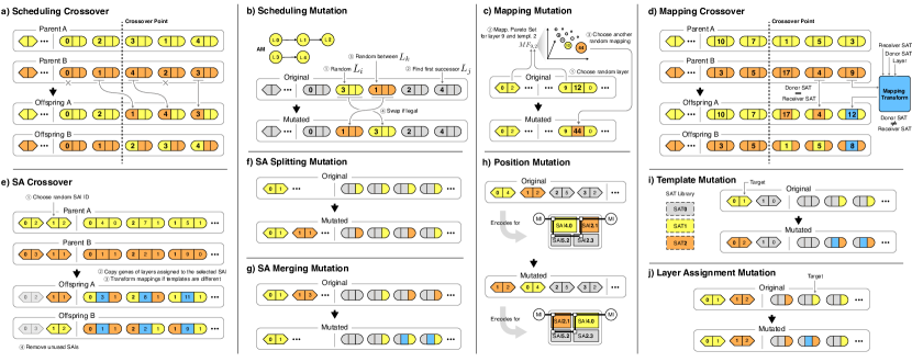
Figure 5: MOHaM-specific genetic operators

One of the most fundamental and important steps in employing a GA is to define an encoding for the individuals in the population. MOHaM requires this encoding to represent, (a) mapping strategy of each layer, (b) $SAI$ of each layer, (c) execution sequence of layers in the $AM(L,D)$, (d) SA template of each $SAI$, and (e) NoP tile of each $SAI$. Hence, the global scheduler uses a two-part chromosome, as shown in Figure 4. The two parts are:

• Software Genome: It encodes the layers of the $AM(L,D)$. It is an array of genes, where each gene denotes a layer. Each gene is a tuple $\langle LI,MI,SAI\rangle$ where $LI$ is the layer identifier, $MI$ is the mapping identifier, and $SAI$ is the SA instance the layer will be executed. The order of the genes is a topological sorting of the layers using Kahn’s algorithm [25] and represents the temporal sequence in which the layers will be executed. The number of genes is equal to the number of layers in the $AM(L,D)$ and is fixed for chromosomes.

• Hardware Genome: It encodes the instances of the $SSAT$. It is an array of genes, where each gene denotes a SA instance. Each gene is a tuple $\langle SAI,SAT\rangle$ where $SAI$ is the SA instance and $SAT$ is the template identifier. The order of the genes represents position of the $SAI$ hosting tile in the 2D Mesh NoP. The number of genes is equal to the number of SA instances and varies between 1 and maximum NoP tiles across chromosomes.

V-B2 Custom Genetic Operators

Each chromosome must respect certain constraints for it to represent a valid individual. For example, the topological sorting of layers in the software genome must be valid. It has to be a traversal where a layer is placed only after all its dependencies. Similarly, the $SAI$ of a layer must refer to one of the encoded genes in the hardware genome. Furthermore, the $MI$ of a layer must refer to one of the mappings in the $MF_{l,f}$. In order to improve the search efficiency, a set of custom genetic operators are implemented that considers these constraints. The operators either avoid generating invalid combinations or use compensation mechanisms. Operators targeting the topological sorting in the software genome are similar to [56]. MOHaM-specific genetic operators are shown in Figure 5 and are described here:

• Scheduling Crossover: It combines the topological sorting of the parent chromosomes, as shown in Figure 5(a). It generates offspring by taking the first part of one of the parents, i.e., all the genes before the crossover point, and appending all the unique genes from the other parent.

• Scheduling Mutation: It mutates the topological sorting of a chromosome, as shown in Figure 5(b). Let $l_{i}$ be a random gene (layer). Let $l_{j}$ be the nearest layer in the traversal that is dependent on $l_{i}$. Let $l_{k}$ be a random gene between $l_{i}$ and $l_{j}$. If all the layers $l_{k}$ has a dependency lie before $l_{i}$ in the traversal, their position can be swapped.

• Mapping Mutation: It modifies the $MI$ of a random layer $l_{i}$ to mutate a chromosome, as shown in Figure 5(c). The possible mappings for a layer will be in the $ML_{l,f}$. One of those mappings is assigned to the $l_{i}$ for mutation.

• Mapping Crossover: It combines the mappings of the parent chromosomes, as shown in Figure 5(d). It generates offspring by taking layer mappings from the first part of one of the parents, i.e., from all the genes before the crossover point, and the remaining ones from the other parent. However, the mapping for a layer (gene) might not be valid if the SA instance is of a different template. In that case, a compensation mechanism called Mapping Transform is applied to find the most similar one among all the possible mappings for the layer in that SA instance.

• SA Crossover: It swaps a random SA instance $s_{i}$ between the parent chromosomes, as shown in Figure 5(e). If both parents A and B have an instance with the same identifier $s_{i}$, they are swapped and two offspring are generated. If $s_{i}$ of A and $s_{i}$ of B are of different SA templates, all the mappings from both of their layers undergo mapping transformation. If $s_{i}$ is only in one of the parents, it is added to the other parent with all its assigned layers. Then only one offspring is generated.

• SA Splitting Mutation: It reduces the load in a random SA instance $s_{i}$ to mutate a chromosome, as shown in Figure 5(f). Another instance $s_{j}$ of the same SA template is appended to the hardware genome. Thereafter, half of the layers currently assigned to $s_{i}$ are randomly chosen and assigned to $s_{j}$. The goal is to increase parallelisation.

• SA Merging Mutation: It increases the load in a random SA instance $s_{i}$ to mutate a chromosome, as shown in Figure 5(g). Another instance $s_{j}$ is randomly chosen, and all the layers currently assigned to it are assigned to $s_{i}$. If $s_{i}$ and $s_{j}$ are of different SA templates, all the mappings of the imported layers undergo mapping transformation. The goal is to reduce chip area cost with reduced SAs.

• SA Position Mutation: It swaps the position of two SAI hosting tiles in the 2D Mesh NoP, as shown in Figure 5(h). The goal is to find a configuration where the system bandwidth is distributed among the NoP links and memory interfaces in a way to avoid bottlenecks (stalls).

• SA Template Mutation: It modifies the $SAT$ of a random SA instance $s_{i}$ to mutate a chromosome, as shown in Figure 5(i). All the mappings from different layers to the mutated instance $s_{i}$ undergo mapping transformation.

• Layer Assignment Mutation: It modifies the $SAI$ of a random layer $l_{i}$ to mutate a chromosome, as shown in Figure 5(j). If the modified $SAI$ is an instance of a different SA template, mapping transformation is applied.

V-C Objectives Evaluation

Three objective metrics are evaluated for each individual: latency, energy, and area. Their values are determined by both, hardware and software genomes of the individual’s chromosome. For example, increasing the number of SA instances decreases latency but increases area. Similarly, the mapping strategy for each layer of the $AM(L,D)$, and the SA templates affect all three metrics. The translation from chromosome encoding to target metrics is not through analytical models. Timeloop [39] + Accelergy [54] framework only allows the simulation of a single layer on a single accelerator instance. Hence, it is repeatedly run for multiple layers and SA instances and the results are combined and processed by MOHaM.

The translation begins from the hardware genome. Each of its genes is converted into a SA instance of the appropriate $SAT$. At this point, the buffer sizes and instances of each $SAT$ is unknown. Then software genomes are examined to identify which mappings are used for each gene (layer). Now all the free parameters, including number of PEs, size of buffers, etc. are set to maximum required by the mappings for all the layers assigned to an SA instance. So, each of the instances can execute all the assigned layers, and the area is estimated.

As each of the mappings has a corresponding energy, summing them for all the layers could provide the total estimation. However, the energy for reads and writes in buffers depends on their sizes. Hence, energy for each mapping must be estimated based on the updated values of the free parameters in the corresponding SA instance. Their sum is the total energy.

Latency is estimated using the topological sorting encoded in the software genome. Each of its genes (layers) is read sequentially and mapped on the assigned SA instances. This traversal guarantees that all the dependencies of a layer are already scheduled before its turn comes. Each layer has a start and end time and the total latency is estimated based on the latest end time among all the layers. However, this is true only when there are no communication or memory bottlenecks.

V-C1 Communication Modeling

As shown in Figure 3(d), MOHaM assumes that the $SAI$s and memory are interconnected by a 2D Mesh NoP. It is implemented via on-package links using a passive silicon interposer. It employs efficient intra-package signalling circuits using Ground-Reference Signaling (GRS) technology. Specifically, each chiplet is equipped with eight chiplet-to-chiplet GRS transceivers; four transmitters and four receivers. A transceiver has four data lanes, each providing 4 GB/s, thus a total peak chiplet bandwidth of 4 * 4 GB/s = 16 GB/s and energy of 0.82 pJ/bit. MOHaM also assumes that the entry points of NoP are Memory Interfaces ($MI$s), which connect memory banks. $SAI$s reads and writes in their nearest $MI$s. Some CPU processing happens between layer execution (e.g. tensor reordering) and the output is stored in the nearest memory bank of the $SAI$ executing the next layer. Depending on their position in the NoP, multiple $SAI$s could be assigned the same $MI$, thus competing for the shared link. If a time segment has parallel execution of layers and the required bandwidth is below the bottleneck, it undergoes temporal dilation. However, it only concerns the $SAI$s sharing the same $MI$ and requires compensating the start times of all the subsequent layers to keep respecting dependencies. After re-evaluating the stalled time segments, the latest end time among all the layers becomes the estimated total latency.

V-C2 Convergence Criterion

The MOHaM framework supports a GA stopping criterion based on the density of the non-dominated solutions presented in [47]. Alternatively, simulating for a fixed number of generations can also be configured.

VI Evaluation

VI-A Methodology

VI-A1 DNN Models and Workloads

Inspired by the popular MLPerf benchmark suite [45][36], multiple DNN models from major application domains like vision, language and recommendation are considered. MOHaM is proposed for design-space exploration of multi-accelerator systems where the application domains are known/guessed apriori. Hence, it is evaluated against mobile, edge, and AR/VR workloads. While these devices do not deploy multi-accelerator systems directly, MOHaM assumes that their heavy workloads are offloaded in the cloud, i.e., data centers. MOHaM is also evaluated against a data center workload to show its effectiveness if the application domains can be guessed. Table 3 presents the workload scenarios along with their DNN models. MOHaM takes them as inputs in the ONNX [1] interoperable format.

VI-A2 Sub-Accelerator Templates

The following state-of-the-art accelerators constitute the $SAT$ library in MOHaM:

• Eyeriss [9]: Row-stationary dataflow

• Simba [50]: Weight-stationary dataflow

• ShiDianNao [15]: Output-stationary dataflow

They are diverse and chosen to support various existing as well emerging workloads. Table 4 presents MOHaM configuration for the experiments, where the GA exploration parameters are based on the guidelines of the widely adopted [16] and architectural parameters are based on the state-of-the-art.

VI-A3 Solution Anatomy

Table 3: Multi-tenant workload scenarios

#	Workload	Domain	DNN Model
A	Mobile	Image Classification	MobileNetV3L
		Image Segmentation	DeepLabV3+ MN2
		Language Processing	Mobile-BERT
B	Edge	Image Classification	ResNet50
		Object Detection	SSD-ResNet34
		Language Processing	BERT-Large
C	AR/VR	Image Classification	ResNet50
		Object Detection	SSD-MobileNetV1
			YOLOv3
		Image Segmentation	UNet
D	Data Center	Image Classification	GoogleNet
		Object Detection	YOLOv3
		Language Processing	BERT-Large
		Recommendation	DLRM

Table 4: MOHaM configuration

Exploration Parameters
Num. Generations	300	Population Size	250
Sched. Cross. Prob.	0.103	Sched. Mut. Prob.	0.052
SA Cross Prob.	0.045	Template Mut. Prob.	0.041
Merging Mut. Prob.	0.042	Splitting Mut. Prob.	0.039
Mapping Mut. Prob.	0.048	Mapping Cross. Prob.	0.047
Layer Assign. Mut. Prob.	0.025	Position Mut. Prob.	0.027
Max. SA Instances	16
Common Architecture Parameters
Technology Node	45 nm	DRAM Technology	LPDDR4
Mem. Interface BW	4 GB/s	Clock Frequency	1 GHz
Word Size	8 bits	SRAM Buf. BW	16 GB/s
Eyeriss-like Template
Dataflow	Row-Stat.	Max. Num. of PEs	168
Max. Shared Buf. Size	131 KiB	Max. PE Scratchpad Size	0.5 KiB
Simba-like Template
Dataflow	Weight-Stat.	Max. Num. of PEs	128
Max. MACs per PE	32	Max. Global Buf. Size	64 KiB
Max. Weight Buf. Size	32 KiB	Max. Input Buf. Size	8 KiB
Max. Accum. Buf. Size	3 KiB
ShiDianNao-like Template
Dataflow	Output-Stat.	Max. Num. of PEs	256
Max. Neurons Buf. Size	131 KiB	Max. Synapses Buf. Size	131 KiB

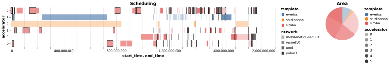
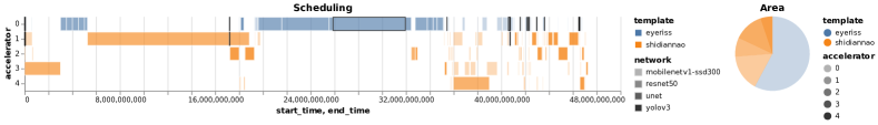
Figure 6: Comparison of scheduling Gantt chart and SA area contribution for two Pareto-optimal solutions.

Figure 6 presents the scheduling Gantt chart and the area breakdown of SA for two Pareto-optimal solutions found by MOHaM for the AR/VR workload. The Gantt chart shows on the y-axis, the instantiated SAs ($SAI$s), and on the x-axis, the start and end times of the execution of each DNN layer, measured in cycles. Each bar represents the execution of a layer of the $AM(L,D)$ on a particular $SAI$. Layers from different DNN models are depicted with different opacity, while layers executed on instances of different $SATs$ are depicted with different colours. Segments with black traces represent bandwidth-constrained execution segments as described in Section V-C1. The pie chart on the right displays the area contribution of each $SAI$ with different opacity, namely the $MAS$ area breakdown. Instances from the same $SAT$ have the same colour. It can be noticed that the two solutions shown here are very different in terms of their scheduling and sub-accelerator instantiation preferences.

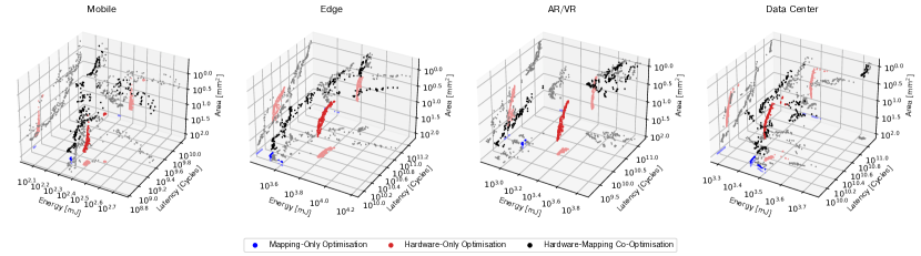
Figure 7: Comparison of Pareto-optimal solutions with hardware-only, mapping-only, and hardware-mapping co-optimisation.

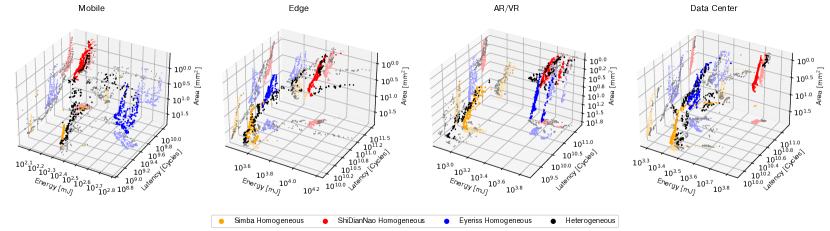
Figure 8: Comparison of Pareto-optimal solutions with homogenous and heterogenous sub-accelerators.

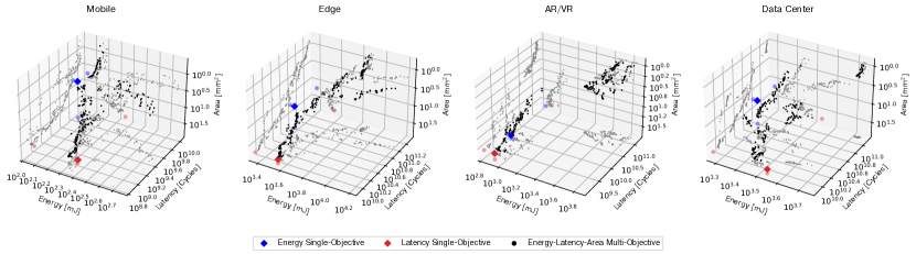
Figure 9: Comparison of individual solutions with mono-objective and Pareto-optimal solutions with multi-objective exploration.

VI-B Results

For all the 3D plots shown in Figures 7, 8 and 9, the more left and top a solution lies, the better it is in performance. For the ease of readability, the plots report the projection of the solution points on three different planes, i.e., latency, energy and area. A common observation valid for all the results presented in this section is the distribution of the solutions found by the proposed MOHaM framework. In fact, they are spread over a large Pareto surface rather than being limited to a specific region. This is an important advantage of MOHaM as it provides a variety of trade-off solutions from which the most appropriate for the specific use case can be selected.

VI-B1 Independent vs Simultaneous Optimisation

This experiment evaluates the need for hardware-mapping co-optimisation in multi-accelerator systems. Figure 7 shows the comparison of Pareto-optimal solutions with hardware-only, mapping-only and hardware-mapping co-optimisation. For hardware-only optimisation, the proposed MOHaM framework is run with only Simba-like SA templates to have a fixed dataflow (e.g., weight-stationary), similar to ConfuciuX [26]. For mapping-only optimisation, MOHaM is run with a fixed hardware configuration of 16 heterogeneous SAs, similar to MAGMA [28]. Finally, they are compared with the result of a complete MOHaM run for hardware-mapping co-optimisation. It is observed that for the AR/VR workload, hardware-only optimisation (red) has lower energy and area but high latency. This is due to the fixed mapping (dataflow) strategy for all the layers. Whereas mapping-only optimisation (blue) has lower latency and energy but at the cost of a very high area. This is due to the fixed hardware configuration. In general, across all the workload scenarios, hardware-only optimisation has better energy and area but poor latency. Similarly, mapping-only optimisation has better latency and energy but high area. With hardware-mapping co-optimisation, the solutions (black) are very interesting. For example, for the Data Center workload, they have solutions with lower latency and energy along with minimum area. They have equally competitive solutions across other workloads. This is a result of the proposed MOHaM framework instantiating the SAs with optimal hardware resources and mapping the layers according to their dataflow preferences for optimal execution. Hardware-mapping co-optimisation can accommodate diverse workloads and offer the best overall performance in a multi-accelerator system.

VI-B2 Homogeneous vs Heterogeneous Accelerators

This experiment evaluates the need for heterogeneous SAs in multi-accelerator systems. Figure 8 shows the comparison of Pareto-optimal solutions with homogeneous and heterogeneous SAs. For homogeneous SAs, the proposed MOHaM framework is run once, each with only Eyeriss-like, Simba-like, and ShiDianNao-like SA templates. Then, they are compared with the result of a complete MOHaM run for heterogeneous SAs. It is observed that for the Mobile workload, Eyeriss (blue) has lower latency and area but at the cost of high energy. On the contrary, ShiDianNao (red) is both energy and area efficient but at the cost of very high latency. For the Edge workload, Simba (yellow) has the best while ShiDianNao has the worst latency, respectively. Eyeriss has lower latency, energy as well as area. In general, among the solutions with homogeneous SAs, Simba has better latency while ShiDianNao has a better area. With heterogeneous SAs, the solutions (black) are more uniformly distributed. For example, for the AR/VR workload, they have solutions with the lowest latency, lowest energy and lowest area. Their solutions are equally good for the Data Center and other workloads. It is possible as layers with specific dataflow preferences can be executed on the appropriate SAs. The proposed MOHaM framework instantiates the right set of SAs from the available templates and maps the layers for efficient execution. Hence, flexible dataflow with heterogeneous SAs increases the scalability of a multi-accelerator system toward diverse and emerging workloads.

VI-B3 Single-Objective vs Multi-Objective Exploration

This experiment evaluates the need for multi-objective exploration in multi-accelerator systems. Figure 9 shows the comparison of individual solutions with mono-objective and Pareto-optimal solutions with multi-objective exploration. For mono-objective exploration, the proposed MOHaM framework is run once, each with only latency, and energy as an objective. Then, they are compared with the result of a complete MOHaM run for multi-objective exploration. When objectives conflict, improving one results in worsening the other. For example, for the Data Center workload, the solution with energy as an objective (blue) is at the extreme left (i.e., best), but the latency and area are worst. Similarly, the solution with latency as an objective (red) is best while the area is worst. A multi-accelerator system design is usually explored with more than one objective. Existing works aggregate them into a single solution (e.g., EDP), which suffers if they conflict. Other commonly used forms of aggregations, like the weighted sum of cost functions, do not allow to explore the non-convex regions of the design space. MOHaM supports distinct multi-objective exploration and provides a Pareto-optimal set of solutions (black). For the same Data Center workload, it provides multiple competitive solutions with the lowest energy, latency and area. Similar solutions are available across all the workloads. Multi-objective exploration helps identify the most suitable design for a multi-accelerator system as per the need.

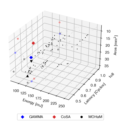
Figure 10: Comparison with state-of-the-art.

VI-B4 Comparison with state-of-the-art

This experiment evaluates MOHaM against two popular state-of-the-art frameworks, CoSA [24] and GAMMA [27]. Like MOHaM, these frameworks also extended Timeloop [39] and are open-sourced, hence considered for a fair comparison. Please note that the simulations for CoSA and GAMMA are conducted using appropriate architectures with flexible dataflows without considering the reconfiguration overheads. Figure 10 shows a subset of Pareto-optimal design points obtained by MOHaM along with the design points by CoSA and GAMMA for the AR/VR workload. MOHaM clearly shows the ability to generate better design points than its competitors. For example, the design point $\blacktriangle$ improves latency by $16.5\%$ and energy by $3.6\%$ compared to CoSA, and latency by $7.1\%$ and energy by $4.7\%$ compared to GAMMA. Based on the specific requirements, other design points can also be considered. For example, if energy is the priority, design point $\blacktriangledown$ improves energy by $21.2\%$ and $22\%$ compared to CoSA and GAMMA, at the cost of $17.3\%$ and $29\%$ decrease in latency, respectively.

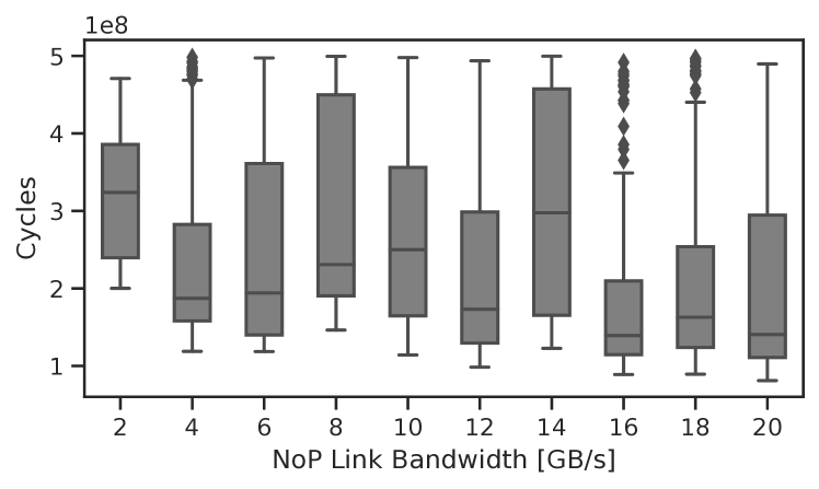
Figure 11: Latency against varying NoP link bandwidth.

VI-B5 Sensitivity of NoP Link Bandwidth

MOHaM calculates latency by combining and processing results of individual Timeloop [39] simulations and considering an NoP for data transfer between $MI$s to $SAI$s. Hence, latency depends on the NoP hosting tile of each $SAI$, the amount of data accessed from memory, determined by the layer mappings, and the NoP link bandwidth. Figure 11 shows the latency of Pareto-optimal design points by MOHaM with varying NoP link bandwidth for the AR/VR workload. Apart from some exceptions due to the stochastic nature of GAs, there is a trend of decreasing latency with increasing bandwidth. However, bandwidth beyond 16 GB/s does not seem to improve the latency significantly.

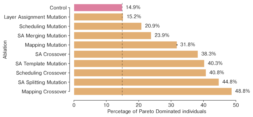
Figure 12: Percentage of Pareto-dominated solutions when an operator is ablated from the baseline MOHaM configuration.

VI-B6 Ablation Study

This experiment evaluates the effectiveness of the custom genetic operators implemented for the MOHaM framework. It compares the result of a complete MOHaM run with the results of runs, each with one operator disabled (ablated). Figure 9 shows the percentage of Pareto-dominated solutions when an operator is ablated from the baseline MOHaM configuration (refer Table 4). Due to the multi-objective exploration, the results are obtained as follows: (a) MOHaM is run with the default configuration, and a baseline Pareto-optimal set of individuals is selected from the final population. (b) MOHaM is re-run with the same configuration to get a second Pareto-optimal set of individuals. (c) They are compared to identify how many individuals from the second set are Pareto-dominated by the individuals from the baseline set. This is found to be 14.9% and serves as the Control setting, as shown in Figure 12. Control serves as the threshold to compare ablation results. (d) MOHaM is run after disabling one custom genetic operator to get a new Pareto-optimal set of individuals. (e) Steps (c) and (d) are repeated for all the operators and the results are presented in Figure 12. A higher percentage of Pareto-dominated individuals indicate that the operator is more effective and that the performance of MOHaM will deteriorate without it. All the operators perform better than the Control threshold, implying that each one of them has some significance in the MOHaM framework.

VII Related Works

DNN Models: Data center workloads are dominated by vision, language and recommendation-based DNN models [7][46][41]. Most of the vision models are dominated by Convolution (CONV) with some MultiLayer Perceptron (MLP) and Fully Connected (FC) layers towards the end [49][52][21][51][31]. Language models are dominated by MLP, Recurrent Neural Network (RNN), embedding lookup and attention layers [13][30][44][42]. Whereas, recommendation models mainly consists of MLP, embedding lookup and attention layers [19][38][22][11]. Design Space Exploration: Hardware optimisations are used at design-time by ASICs or even at compile-time by FPGAs. Literature has multiple heuristic as well as ML-based hardware frameworks [37][26]. Mapping optimisations are used at compile-time or even at run-time by reconfigurable accelerators. Literature has mapping frameworks based on heuristics [57], random search [50], mixed integer programming [24], ML [55], etc. Hardware-mapping co-optimisations are used at design-time. Due to the huge cross-coupled search space, very few works have explored co-optimisation for single [58][29][48][55][57] and multi-accelerator systems [33][18]. Multi-Tenancy: Until recently, multi-tenancy has not been an important design choice for accelerators. Google TPU [5], Microsoft Brainwave [17], etc., focused on running a single DNN model for maximum throughput. The popular MLPerf benchmark suite also focused on a single model for both, training [36] and inference [45]. Data centers are now employing multi-accelerator systems where throughput is not the only objective. Moreover, they have the natural ability to support diverse DNN models as each SA could favour a specific layer. Hence, multi-tenancy has garnered significant attention recently [28][35][33][18][12][8].

VIII Discussion

MOHaM is used offline at design time to obtain a Pareto-optimal set of $MAS$ and an optimal $S$ for each of them. Hence its search time is irrelevant to the performance of the chosen $MAS$ and $S$. When the $MAS$ is deployed, it is assumed to employ batch processing, which is very common in data centers. A batch may have DNN models from heterogeneous application domains. Based on their specific requirements, $S$ schedules these models on the heterogenous $SAI$s of the $MAS$. What might seem just like multi-workload scheduling is also multi-tenant, as heterogeneous DNN models execute in parallel. MOHaM uses $SAT$s with fixed dataflow as state-of-the-art Herald [33] found them better over $SAT$s with flexible dataflow. Nevertheless, MOHaM is can deal with flexible dataflow and full mapping search. Any $SAT$ that Timeloop [39] supports can be given as an input to MOHaM.

IX Conclusion

This work presents MOHaM, a multi-objective hardware-mapping co-optimisation framework for multi-tenant DNN accelerators. The key takeaways are: (1) The ever-increasing computation demand led to the design of multi-accelerator systems, where hardware-mapping co-optimisation is very important. However, due to the enormous cross-coupled search space, very few works explored the design space (refer Table 1). (2) Multi-tenancy is a primary enabler of scalability in multi-accelerator systems. However, most of the existing works employ manually-designed supports that limit accelerator utilisation and deployment benefits. (3) Multi-accelerator systems are often designed for multiple objectives, yet no work exists for multi-objective exploration. (4) MOHaM is the first open-source framework to consider all these limitations. (5) MOHaM also has infrastructure for NoP/data movement.

References

- [1] “Open Neural Network Exchange (ONNX),” https://github.com/onnx/onnx, 2017.
- [2] “Google Edge TPUv1,” https://cloud.google.com/edge-tpu/, 2018.
- [3] (2018) NVDIA Deep Learning Accelerator (NVDLA). http://nvdla.org/.
- [4] (2021) Cerebras CS-2. https://cerebras.net/system/.
- [5] (2021) Google Cloud TPUv4. https://cloud.google.com/tpu/.
- [6] A. Aimar, H. Mostafa, E. Calabrese, A. Rios-Navarro, R. Tapiador-Morales, I.-A. Lungu, M. B. Milde, F. Corradi, A. Linares-Barranco, S.-C. Liu et al., “NullHop: A Flexible Convolutional Neural Network Accelerator based on Sparse Representations of Feature Maps,” IEEE Transactions on Neural Networks and Learning Systems, vol. 30, no. 3, pp. 644–656, 2018.
- [7] M. Anderson, B. Chen, S. Chen, S. Deng, J. Fix, M. Gschwind, A. Kalaiah, C. Kim, J. Lee, and J. a. Liang, “First-Generation Inference Accelerator Deployment at Facebook,” arXiv preprint arXiv:2107.04140, 2021.
- [8] E. Baek, D. Kwon, and J. Kim, “A Multi-Neural Network Acceleration Architecture,” in Proceedings of the Annual ACM/IEEE International Symposium on Computer Architecture, 2020, pp. 940–953.
- [9] Y.-H. Chen, T. Krishna, J. S. Emer, and V. Sze, “Eyeriss: An Energy-Efficient Reconfigurable Accelerator for Deep Convolutional Neural Networks,” IEEE Journal of Solid-State Circuits, vol. 52, no. 1, pp. 127–138, 2016.
- [10] Y.-H. Chen, T.-J. Yang, J. Emer, and V. Sze, “Eyeriss v2: A Flexible Accelerator for Emerging Deep Neural Networks on Mobile Devices,” IEEE Journal on Emerging and Selected Topics in Circuits and Systems, vol. 9, no. 2, pp. 292–308, 2019.
- [11] H.-T. Cheng, L. Koc, J. Harmsen, T. Shaked, T. Chandra, H. Aradhye, G. Anderson, G. Corrado, W. Chai, M. Ispir et al., “Wide & Deep Learning for Recommender Systems,” in Proceedings of the Annual Workshop on Deep Learning for Recommender Systems, 2016, pp. 7–10.
- [12] Y. Choi and M. Rhu, “PREMA: A Predictive Multi-Task Scheduling Algorithm for Preemptible Neural Processing Units,” in Proceedings of the Annual IEEE International Symposium on High Performance Computer Architecture, 2020, pp. 220–233.
- [13] Z. Dai, Z. Yang, Y. Yang, J. G. Carbonell, Q. Le, and R. Salakhutdinov, “Transformer-XL: Attentive Language Models beyond a Fixed-Length Context,” in Proceedings of the Annual Meeting of the Association for Computational Linguistics, 2019, pp. 2978–2988.
- [14] K. Deb, A. Pratap, S. Agarwal, and T. Meyarivan, “A Fast and Elitist Multiobjective Genetic Algorithm: NSGA-II,” IEEE Transactions on Evolutionary Computation, vol. 6, no. 2, pp. 182–197, 2002.
- [15] Z. Du, R. Fasthuber, T. Chen, P. Ienne, L. Li, T. Luo, X. Feng, Y. Chen, and O. Temam, “ShiDianNao: Shifting Vision Processing Closer to the Sensor,” in Proceedings of the Annual ACM/IEEE International Symposium on Computer Architecture, 2015, pp. 92–104.
- [16] A. E. Eiben and S. K. Smit, “Parameter Tuning for Configuring and Analyzing Evolutionary Algorithms,” Elsevier Swarm and Evolutionary Computation, vol. 1, no. 1, pp. 19–31, 2011.
- [17] J. Fowers, K. Ovtcharov, M. Papamichael, T. Massengill, M. Liu, D. Lo, S. Alkalay, M. Haselman, L. Adams, M. Ghandi et al., “A Configurable Cloud-Scale DNN Processor for Real-Time AI,” in Proceedings of the Annual ACM/IEEE International Symposium on Computer Architecture, 2018, pp. 1–14.
- [18] S. Ghodrati, B. H. Ahn, J. K. Kim, S. Kinzer, B. R. Yatham, N. Alla, H. Sharma, M. Alian, E. Ebrahimi, N. S. Kim et al., “Planaria: Dynamic Architecture Fission for Spatial Multi-Tenant Acceleration of Deep Neural Networks,” in Proceedings of the Annual IEEE/ACM International Symposium on Microarchitecture, 2020, pp. 681–697.
- [19] U. Gupta, S. Hsia, V. Saraph, X. Wang, B. Reagen, G.-Y. Wei, H.-H. S. Lee, D. Brooks, and C.-J. Wu, “DeepRecSys: A System for Optimizing End-to-End At-Scale Neural Recommendation Inference,” in Proceedings of the Annual ACM/IEEE International Symposium on Computer Architecture, 2020, pp. 982–995.
- [20] S. Han, X. Liu, H. Mao, J. Pu, A. Pedram, M. A. Horowitz, and W. J. Dally, “EIE: Efficient Inference Engine on Compressed Deep Neural Network,” ACM SIGARCH Computer Architecture News, vol. 44, no. 3, pp. 243–254, 2016.
- [21] K. He, X. Zhang, S. Ren, and J. Sun, “Deep Residual Learning for Image Recognition,” in Proceedings of the Annual IEEE/CVF Conference on Computer Vision and Pattern Recognition, 2016, pp. 770–778.
- [22] X. He, L. Liao, H. Zhang, L. Nie, X. Hu, and T.-S. Chua, “Neural collaborative filtering,” in Proceedings of the Annual ACM International Conference on World Wide Web, 2017, pp. 173–182.
- [23] K. Hegde, P.-A. Tsai, S. Huang, V. Chandra, A. Parashar, and C. W. Fletcher, “Mind Mappings: Enabling Efficient Algorithm-Accelerator Mapping Space Search,” in Proceedings of the Annual ACM International Conference on Architectural Support for Programming Languages and Operating Systems, 2021, pp. 943–958.
- [24] Q. Huang, A. Kalaiah, M. Kang, J. Demmel, G. Dinh, J. Wawrzynek, T. Norell, and Y. S. Shao, “CoSA: Scheduling by Constrained Optimization for Spatial Accelerators,” in Proceedings of the Annual ACM/IEEE International Symposium on Computer Architecture, 2021, pp. 554–566.
- [25] A. B. Kahn, “Topological Sorting of Large Networks,” Communications of the ACM, vol. 5, no. 11, pp. 558–562, 1962.
- [26] S.-C. Kao, G. Jeong, and T. Krishna, “ConfuciuX: Autonomous Hardware Resource Assignment for DNN Accelerators using Reinforcement Learning,” in Proceedings of the Annual IEEE/ACM International Symposium on Microarchitecture, 2020, pp. 622–636.
- [27] S.-C. Kao and T. Krishna, “Gamma: Automating the HW Mapping of DNN Models on Accelerators via Genetic Algorithm,” in Proceedings of the Annual IEEE/ACM International Conference On Computer Aided Design, 2020, pp. 1–9.
- [28] S.-C. Kao and T. Krishna, “MAGMA: An Optimization Framework for Mapping Multiple DNNs on Multiple Accelerator Cores,” in Proceedings of the Annual IEEE International Symposium on High-Performance Computer Architecture, 2022, pp. 1–17.
- [29] S.-C. Kao, M. Pellauer, A. Parashar, and T. Krishna, “DiGamma: Domain-Aware Genetic Algorithm for HW-Mapping Co-Optimization for DNN Accelerators,” in Proceedings of the Annual IEEE Design, Automation & Test in Europe Conference & Exhibition, 2022, pp. 1–6.
- [30] J. D. M.-W. C. Kenton and L. K. Toutanova, “BERT: Pre-training of Deep Bidirectional Transformers for Language Understanding,” in Proceedings of the Annual Conference of the North American Chapter of the Association for Computational Linguistics, 2019, pp. 4171–4186.
- [31] A. Krizhevsky, I. Sutskever, and G. E. Hinton, “ImageNet Classification with Deep Convolutional Neural Networks,” in Proceedings of the Annual Conference on Neural Information Processing Systems, 2012, pp. 1097––1105.
- [32] H. Kwon, P. Chatarasi, M. Pellauer, A. Parashar, V. Sarkar, and T. Krishna, “Understanding Reuse, Performance, and Hardware Cost of DNN Dataflow: A Data-Centric Approach,” in Proceedings of the Annual IEEE/ACM International Symposium on Microarchitecture, 2019, pp. 754–768.
- [33] H. Kwon, L. Lai, M. Pellauer, T. Krishna, Y.-H. Chen, and V. Chandra, “Heterogeneous Dataflow Accelerators for Multi-DNN Workloads,” in Proceedings of the Annual IEEE International Symposium on High-Performance Computer Architecture, 2021, pp. 71–83.
- [34] H. Kwon, A. Samajdar, and T. Krishna, “MAERI: Enabling Flexible Dataflow Mapping over DNN Accelerators via Reconfigurable Interconnects,” in Proceedings of the Annual ACM International Conference on Architectural Support for Programming Languages and Operating Systems, 2018, pp. 461–475.
- [35] Z. Liu, J. Leng, Z. Zhang, Q. Chen, C. Li, and M. Guo, “VELTAIR: Towards High-Performance Multi-Tenant Deep Learning Services via Adaptive Compilation and Scheduling,” in Proceedings of the Annual ACM International Conference on Architectural Support for Programming Languages and Operating Systems, 2022, pp. 1–14.
- [36] P. Mattson, C. Cheng, G. Diamos, C. Coleman, P. Micikevicius, D. Patterson, H. Tang, G.-Y. Wei, P. Bailis, V. Bittorf et al., “MLPerf Training Benchmark,” in Proceedings of the Annual Conference on Machine Learning and Systems, 2020, pp. 336–349.
- [37] A. Mirhoseini, A. Goldie, M. Yazgan, J. W. Jiang, E. Songhori, S. Wang, Y.-J. Lee, E. Johnson, O. Pathak, A. Nazi et al., “A Graph Placement Methodology for Fast Chip Design,” Nature, vol. 594, no. 7862, pp. 207–212, 2021.
- [38] M. Naumov, D. Mudigere, H.-J. M. Shi, J. Huang, N. Sundaraman, J. Park, X. Wang, U. Gupta, C.-J. Wu, A. G. Azzolini et al., “Deep Learning Recommendation Model for Personalization and Recommendation Systems,” arXiv preprint arXiv:1906.00091, 2019.
- [39] A. Parashar, P. Raina, Y. S. Shao, Y.-H. Chen, V. A. Ying, A. Mukkara, R. Venkatesan, B. Khailany, S. W. Keckler, and J. Emer, “Timeloop: A Systematic Approach to DNN Accelerator Evaluation,” in Proceedings of the Annual IEEE International Symposium on Performance Analysis of Systems and Software, 2019, pp. 304–315.
- [40] A. Parashar, M. Rhu, A. Mukkara, A. Puglielli, R. Venkatesan, B. Khailany, J. Emer, S. W. Keckler, and W. J. Dally, “SCNN: An Accelerator for Compressed-Sparse Convolutional Neural Networks,” ACM SIGARCH Computer Architecture News, vol. 45, no. 2, pp. 27–40, 2017.
- [41] J. Park, M. Naumov, P. Basu, S. Deng, A. Kalaiah, D. Khudia, J. Law, P. Malani, A. Malevich, S. Nadathur et al., “Deep Learning Inference in Facebook Data Centers: Characterization, Performance Optimizations and Hardware Implications,” arXiv preprint arXiv:1811.09886, 2018.
- [42] M. E. Peters, M. Neumann, M. Iyyer, M. Gardner, C. Clark, K. Lee, and L. Zettlemoyer, “Deep Contextualized Word Representations,” pp. 2227–2237, 2018.
- [43] E. Qin, A. Samajdar, H. Kwon, V. Nadella, S. Srinivasan, D. Das, B. Kaul, and T. Krishna, “SIGMA: A Sparse and Irregular GEMM Accelerator with Flexible Interconnects for DNN Training,” in Proceedings of the Annual IEEE International Symposium on High-Performance Computer Architecture, 2020, pp. 58–70.
- [44] A. Radford, J. Wu, R. Child, D. Luan, D. Amodei, I. Sutskever et al., “Language Models are Unsupervised Multitask Learners,” OpenAI Blog, vol. 1, no. 8, p. 9, 2019.
- [45] V. J. Reddi, C. Cheng, D. Kanter, P. Mattson, G. Schmuelling, C.-J. Wu, B. Anderson, M. Breughe, M. Charlebois, W. Chou et al., “MLPerf Inference Benchmark,” in Proceedings of the Annual ACM/IEEE International Symposium on Computer Architecture, 2020, pp. 446–459.
- [46] D. Richins, D. Doshi, M. Blackmore, A. T. Nair, N. Pathapati, A. Patel, B. Daguman, D. Dobrijalowski, R. Illikkal, K. Long et al., “Missing the Forest for the Trees: End-to-End AI Application Performance in Edge Data Centers,” in Proceedings of the Annual IEEE International Symposium on High-Performance Computer Architecture, 2020, pp. 515–528.
- [47] O. Roudenko and M. Schoenauer, “A Steady Performance Stopping Criterion for Pareto-based Evolutionary Algorithms,” in Proceedings of the Annual International Multi-Objective Programming and Goal Programming Conference, 2004.
- [48] E. Russo, M. Palesi, S. Monteleone, D. Patti, G. Ascia, and V. Catania, “MEDEA: A Multi-Objective Evolutionary Approach to DNN Hardware Mapping,” in Proceedings of the Annual IEEE Design, Automation & Test in Europe Conference & Exhibition, 2022, pp. 1–6.
- [49] M. Sandler, A. Howard, M. Zhu, A. Zhmoginov, and L.-C. Chen, “MobileNetV2: Inverted Residuals and Linear Bottlenecks,” in Proceedings of the Annual IEEE/CVF Conference on Computer Vision and Pattern Recognition, 2018, pp. 4510–4520.
- [50] Y. S. Shao, J. Clemons, R. Venkatesan, B. Zimmer, M. Fojtik, N. Jiang, B. Keller, A. Klinefelter, N. Pinckney, P. Raina, S. G. Tell, Y. Zhang, W. J. Dally, J. Emer, and C. T. Gray, “Simba: Scaling Deep-Learning Inference with Multi-Chip-Module-Based Architecture,” in Proceedings of the Annual IEEE/ACM International Symposium on Microarchitecture, 2019, pp. 14–27.
- [51] K. Simonyan and A. Zisserman, “Very Deep Convolutional Networks for Large-Scale Image Recognition,” arXiv preprint arXiv:1409.1556, 2014.
- [52] C. Szegedy, S. Ioffe, V. Vanhoucke, and A. A. Alemi, “Inception-v4, Inception-ResNet and the Impact of Residual Connections on Learning,” in Proceedings of the Annual AAAI Conference on Artificial Intelligence, 2017.
- [53] J. Wang, L. Guo, and J. Cong, “AutoSA: A Polyhedral Compiler for High-Performance Systolic Arrays on FPGA,” in Proceedings of the Annual ACM/SIGDA International Symposium on Field-Programmable Gate Arrays, 2021, pp. 93–104.
- [54] Y. N. Wu, J. S. Emer, and V. Sze, “Accelergy: An architecture-level energy estimation methodology for accelerator designs,” in 2019 IEEE/ACM International Conference on Computer-Aided Design (ICCAD). IEEE, 2019, pp. 1–8.
- [55] Q. Xiao, S. Zheng, B. Wu, P. Xu, X. Qian, and Y. Liang, “HASCO: Towards Agile Hardware and Software Co-Design for Tensor Computation,” in Proceedings of the Annual ACM/IEEE International Symposium on Computer Architecture, 2021, pp. 1055–1068.
- [56] Y. Xu, K. Li, J. Hu, and K. Li, “A Genetic Algorithm for Task Scheduling on Heterogeneous Computing Systems using Multiple Priority Queues,” Elsevier Information Sciences, vol. 270, pp. 255–287, 2014.
- [57] X. Yang, M. Gao, Q. Liu, J. Setter, J. Pu, A. Nayak, S. Bell, K. Cao, H. Ha, P. Raina et al., “Interstellar: Using Halide’s Scheduling Language to Analyze DNN Accelerators,” in Proceedings of the Annual ACM International Conference on Architectural Support for Programming Languages and Operating Systems, 2020, pp. 369–383.
- [58] D. Zhang, S. Huda, E. Songhori, K. Prabhu, Q. Le, A. Goldie, and A. Mirhoseini, “A Full-Stack Search Technique for Domain Optimized Deep Learning Accelerators,” in Proceedings of the Annual ACM International Conference on Architectural Support for Programming Languages and Operating Systems, 2022, pp. 27–42.