Masked Modeling Duo: Learning Representations
by Encouraging Both Networks to Model the Input

Abstract

Masked Autoencoders is a simple yet powerful self-supervised learning method. However, it learns representations indirectly by reconstructing masked input patches. Several methods learn representations directly by predicting representations of masked patches; however, we think using all patches to encode training signal representations is suboptimal. We propose a new method, Masked Modeling Duo (M2D), that learns representations directly while obtaining training signals using only masked patches. In the M2D, the online network encodes visible patches and predicts masked patch representations, and the target network, a momentum encoder, encodes masked patches. To better predict target representations, the online network should model the input well, while the target network should also model it well to agree with online predictions. Then the learned representations should better model the input. We validated the M2D by learning general-purpose audio representations, and M2D set new state-of-the-art performance on tasks such as UrbanSound8K, VoxCeleb1, AudioSet20K, GTZAN, and SpeechCommandsV2.

Index Terms—  Self-supervised learning, Masked Autoencoders, Masked Image Modeling, Masked Spectrogram Modeling

1 Introduction

Recently, self-supervised learning (SSL) methods using masked image modeling (MIM) have progressed and yielded promising results in the image domain. Among them, Masked Autoencoders[1] (MAE) have inspired numerous subsequent studies and influenced not only the image domain[2, 3, 4, 5] but also the audio domain[6, 7, 8, 9].

An MAE effectively learns a representation by reconstructing a large number (i.e., 75%) of masked input patches using a small number of visible patches, encouraging the learned representation to model the input. However, it learns representations indirectly by minimizing the loss between the original input and the reconstructed result, which may not be optimal for learning a representation.

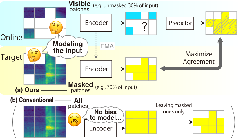
Fig. 1: M2D pre-training scenario. The online network encodes visible patches and predicts masked patch representations, while the target network encodes masked patches. The M2D maximizes the agreement between these two outputs to learn representations. We provide only the masked patches to the target illustrated as (a), unlike conventional methods (e.g., data2vec[10]) depicted as (b), encouraging representations to model the input from both the online and target networks.

In contrast, several previous methods[2, 3, 10] achieve direct learning of representations, typically by using a momentum encoder in a Siamese architecture[11] to obtain the masked patch representations as a training signal. In this case, all input patches are used to encode these representations, not encouraging to model the input.

We hypothesize that the learned representation would become more useful if the training signal were encoded using only masked patches instead of all patches in order to encourage modeling the input in the training signal. While an MAE effectively encourages modeling the input signal by limiting the number of visible patches fed to the encoder, using all the input patches to obtain a training signal does not benefit from the inductive bias of the MAE.

In this paper, we propose a new method, Masked modeling duo (M2D), that learns representations directly by predicting the representations of masked patches from visible patches only. As illustrated in Fig.1, the target representations are encoded from only the masked patches, not from all the input patches as they are in the previous methods[2, 3, 10]. Although our method adds a target momentum encoder to the MAE, the entire framework remains simple.

The M2D promotes complementary input modeling by feeding mutually exclusive patches to its networks. For example, to reduce the prediction error for a heartbeat audio input consisting of two sounds (S1 and S2), the online network should encode the given visible patches around S2 into representations modeled as part of the whole heartbeat in order to predict the representations of masked patches around S1. Conversely, the masked patch representations around S1 encoded by the target network are more likely to agree with the prediction if it is encoded as part of the whole heartbeat. Therefore, our method encourages input modeling from both sides.

In our experiments, we validated our method by learning a general-purpose audio representation using an audio spectrogram as input and confirmed the effectiveness of learning the representation directly and providing only masked patches to the target. In addition, M2D set new state-of-the-art (SOTA) performance on several audio tasks. Our code is available online.

2 Related Work

This study was inspired by MAE[1] for an MIM and Bootstrap Your Own Latent[12] (BYOL) as a framework for directly learning latent representations using a target network. An MAE learns to reconstruct the input data, whereas our M2D learns to predict masked latent representations. BYOL differs from ours in that it is a framework for learning representations invariant to data augmentation.

SIM[2], MSN[3], and data2vec[10] learn to predict masked patch representations using a target network, but, unlike ours, all input patches are fed to the target. CAE[4] and SplitMask[5] encode target representation using only masked patches, which is similar to ours but without the use of a target network. While SIM, MSN, CAE, and SplitMask learn image representations, data2vec also learns audio representations.

In this work, we experimented through learning general-purpose audio representations. To learn speech and audio, various methods learn representations using masked input, such as Mockingjay[13], wav2vec2[14], HuBERT[15], and BigSSL[16] for speech, and SSAST[17] for audio. Methods more closely related to ours are MAE-AST[7], MaskSpec[8], MSM-MAE[9], and Audio-MAE[6], which adapt MAE to learn audio representations. However, they differ from our method in that they do not use a target network.

Other SSL methods for learning audio representations include Wang et al.[18] and DeLoRes[19], and especially BYOL-A[20], BYOL-S[21], and ATST[22], which use BYOL as the learning framework; they do not mask the input. For supervised learning, AST[23], EAT[24], PaSST[25], and HTS-AT[26] have shown SOTA performance.

3 Masked Modeling Duo

Our method learns representations by using only visible patches to predict the masked patch representations. As shown in Fig. 2, it consists of two networks, referred to as the online and target networks.

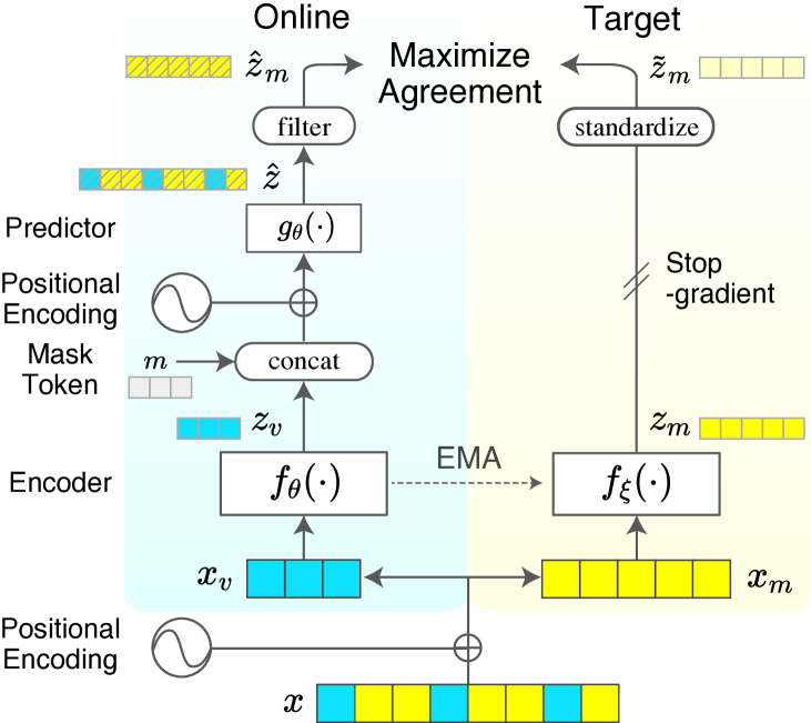
Fig. 2: Overview of the M2D framework.

Processing input   The framework partitions the input data $x$ (audio spectrogram, image, etc.) into a grid of patches, adds positional encoding, and randomly selects a number of patches according to a masking ratio as masked patches $x_{m}$ (e.g., 60% of the input) and the rest as visible patches $x_{v}$ (e.g., the remaining 40%). While we use the same positional encoding as MAE[1], we tested various masking ratios as discussed in Section 4.4.

Online and target networks   The online network, defined by a set of weights $\theta$, encodes the visible patches $x_{v}$ using the online encoder $f_{\theta}$ into the representation $z_{v}=f_{\theta}(x_{v})$. It concatenates shared, learnable masked tokens $m$ to $z_{v}$, adds the position encoding $p$, and predicts $\hat{z}$, representations of entire input patches, using the predictor $g_{\theta}$.

$$\hat{z}=g_{\theta}(\text{concat}(z_{v},m)+p)$$ (1)

It then filters the prediction result $\hat{z}$ to output $\hat{z}_{m}=\{\,\hat{z}[i]\mid i\in I_{M}\,\}$, containing only masked patch representations, where $I_{M}$ is the set of indices of the masked patches.

The target network is defined by parameter $\xi$ and consists only of momentum encoder $f_{\xi}$, which is identical to the online encoder except for the parameter. The network encodes masked patches $x_{m}$ using $f_{\xi}$ to output the representation $z_{m}=f_{\xi}(x_{m})$. We then standardize $z_{m}$ to $\tilde{z}_{m}=({z_{m}-\text{mean}{(z_{m})}})/{\sqrt{\text{var}{(z_{m})}}}$, for stabilizing the training, which we empirically confirmed in preliminary experiments, rather than for performance gain as in MAE.

Calculating loss   The loss is calculated using the standardized target output $\tilde{z}_{m}$ as a training signal against the online prediction output $\hat{z}_{m}$. Inspired by BYOL[12], we calculate the loss $L$ by the mean square error (MSE) of $l_{2}$-normalized $\hat{z}_{m}$ and $\tilde{z}_{m}$.

$$L\triangleq||l_{2}(\hat{z}_{m})-l_{2}(\tilde{z}_{m})||^{2}_{2}=2-2\cdot\frac{\langle\hat{z}_{m},\tilde{z}_{m}\rangle}{||\hat{z}_{m}||_{2}\cdot||\tilde{z}_{m}||_{2}},$$ (2)

where $\langle\cdot,\cdot\rangle$ denotes the inner product.

Updating network parameters   Our framework updates parameters $\theta$ and $\xi$ after each training step. It updates $\theta$ only by minimizing the loss $L$ as depicted by the stop-gradient in Fig. 2, whereas updating $\xi$ is based on a slowly moving exponential average of $\theta$ with a decay rate $\tau$:

$$\xi\leftarrow\tau\xi+(1-\tau)\theta$$ (3)

It has been empirically shown that stop-gradient operation can avoid collapsing to an uninformative solution, and the moving-average behavior may lead to learning effective representations[11]. After the training, we transfer only the $f_{\theta}$ as a pre-trained model.

4 Experiments

We validated the M2D step-by-step experiments that examined the effectiveness of learning representations directly by comparing our M2D with MAE (Section 4.2), the effectiveness of feeding only masked patches to the target (Section 4.3), the impact of various masking ratios (Section 4.4), and comparing ours with SOTA (Section 4.5).

In all experiments, we applied our M2D to masked spectrogram modeling (MSM)[9], with an audio spectrogram as input to learn general-purpose audio representations. We evaluated the performance of pre-trained models in both a linear evaluation and fine-tuning on a variety of audio downstream tasks spanning environmental sounds, speech, and music.

Table 1: Fine-tuning and linear evaluation results. AS20K result is an mAP, and all others are accuracies (%) with 95% CI.

	(a) Fine-tuning				(b) Linear evaluation
					Env. sound tasks		Speech tasks				Music tasks
Model	AS20K	ESC-50	SPCV2	VC1	ESC-50	US8K	SPCV2	VC1	VF	CRM-D	GTZAN	NSynth	Surge	Avg.
MSM-MAE[9]	36.7 $\pm$ 0.5	94.0 $\pm$ 0.2	98.4 $\pm$ 0.1	95.3 $\pm$ 0.1	88.6 $\pm$ 1.5	86.3 $\pm$ 0.3	94.5 $\pm$ 0.2	72.2 $\pm$ 0.2	97.5 $\pm$ 0.1	70.2 $\pm$ 1.1	78.4 $\pm$ 2.8	75.9 $\pm$ 0.2	42.5 $\pm$ 0.7	78.5 $\pm$ 0.8
M2D ratio=0.6	36.8 $\pm$ 0.1	94.7 $\pm$ 0.3	98.5 $\pm$ 0.0	94.8 $\pm$ 0.1	89.7 $\pm$ 0.2	87.6 $\pm$ 0.2	95.4 $\pm$ 0.1	73.1 $\pm$ 0.1	97.9 $\pm$ 0.1	71.7 $\pm$ 0.3	83.3 $\pm$ 1.0	75.3 $\pm$ 0.1	41.0 $\pm$ 0.2	79.5 $\pm$ 0.3
M2D ratio=0.7	37.4 $\pm$ 0.1	95.0 $\pm$ 0.2	98.5 $\pm$ 0.1	94.4 $\pm$ 1.3	89.8 $\pm$ 0.3	87.1 $\pm$ 0.3	94.5 $\pm$ 0.1	71.3 $\pm$ 0.4	97.7 $\pm$ 0.1	71.6 $\pm$ 0.3	83.9 $\pm$ 1.4	76.9 $\pm$ 1.3	41.8 $\pm$ 0.4	79.4 $\pm$ 0.5

4.1 Experimental Setup

We mainly focused on comparing M2D with an MAE, then adapted MAE implementations and settings with as few changes as possible. We implemented an additional target network on top of the MAE code and adopted the MAE decoder as our predictor $g_{\theta}$ without changes. We used vanilla ViT-Base[27] with a 768-d output feature as our encoders ($f_{\theta}$ and $f_{\xi}$) and fixed the patch size to $16\times 16$ for all experiments. We tested with masking ratios of 0.6 and 0.7, which showed good performance in preliminary experiments.

We used the MSM-MAE[9] as an MAE for comparison, an MAE variant optimized for MSM by making the decoder smaller with four layers, six heads, and a width (embedding dimension) of 384-d. Other parameters, including a default masking ratio of 0.75, were the same as in the original MAE. Preliminary experiments verified that the MSM-MAE outperforms a vanilla MAE with an eight-layer decoder.

We employed the MSM-MAE feature calculation in evaluations to optimize M2D representations for MSM as in MSM-MAE. The MSM-MAE outputs $z^{\prime}\in R^{B\times N_{T}\times N_{F}D}$ by concatenating the features of frequency bins for each time frame, instead of simply averaging the $z\in R^{B\times N_{F}N_{T}\times D}$ output from ViT, where $B$ is batch size, $N_{F}$ is the number of patches along frequency, $N_{T}$ is the number of patches along time, and $D$ is a patch feature dimension. Then, we summarized an audio sample level feature $z^{\prime\prime}=1/N_{T}\sum_{t=1}^{N_{T}}z^{\prime}[t]$, averaging $z^{\prime}$ over time. The $z^{\prime\prime}$ becomes a 3,840-d feature, where $D=768$ and $N_{F}=5$.

We preprocessed audio samples to a log-scaled mel spectrogram with a sampling frequency of 16,000 Hz, window size of 25 ms, hop size of 10 ms, and mel-spaced frequency bins $F=80$ in the range of 50 to 8,000 Hz and normalized them with a dataset statistics. All downstream task audios were cropped to the dataset’s average duration or added with zero padding at the end. Long audio samples were split into the input length of the model without overlapping, encoded to $z^{\prime}$ each, concatenated along time, and averaged over time to an audio sample level feature $z^{\prime\prime}$.

Pre-training details   The input audio duration of the ViT used in the experiments was set to 6s, the same as ATST, for comparison with the SOTA methods. The input spectrogram has a size of $80\times 608$ (Freq. bins $\times$ Time frames), making $N_{F}=80/16=5$ and $N_{T}=608/16=38$ with a patch size of $16\times 16$.

We set the number of epochs as 300, warm-up epochs as 20, batch size as 2048, and the base learning rate as 3e-4. All other settings were the same as in the MAE, including the learning rate scheduling and optimizer. The EMA decay rate $\tau$ for the target network update was linearly interpolated from 0.99995 at the start of training to 0.99999 at the end. We used AudioSet[28] as a pre-training dataset with 2,005,132 samples (5,569 h) of 10s audio from the balanced and unbalanced train segments. We randomly cropped 6s audio from a 10s sample. All these settings were common in the M2D and MSM-MAE pre-training, except for the EMA decay rate.

Linear evaluation details   In the linear evaluation, we trained a linear classifier on top of frozen pre-trained models, and tested the performance on a variety of downstream tasks.

All evaluation details and downstream tasks are the same as in our previous study[20]. Tasks include environmental sound classification ESC-50[29] and UrbanSound8K[30] (US8K), speech-command classification Speech Commands V2[31] (SPCV2), speaker identification VoxCeleb1[32] (VC1), language identification VoxForge[33] (VF), speech emotion recognition CREMA-D[34] (CRM-D), music genre recognition GTZAN[35], musical instrument classification NSynth[36], and a pitch audio classification Pitch Audio Dataset (Surge synthesizer)[37]. All the tasks are classification problems, and all the results are accuracies.

Fine-tuning details   We used the tasks commonly used in previous studies: ESC-50, SPCV2, and VC1, the same as in the linear evaluation, plus AudioSet20K (AS20K), which learns only the balanced train segments of AudioSet[28] and results in a mean average pooling (mAP) of multi-label classification with 527 classes.

The fine-tuning pipeline follows ATST. A linear classifier was added on top of the pre-trained model to train the entire network. All evaluations were trained for 200 epochs, and the learning rate was optimized for each task and scheduled with cosine annealing[38] after five epochs of warm-up. We used SGD and AdamW for the optimizer, Mixup[39, 20], Random Resize Crop (RRC)[20] for data augmentation, and Structured Patchout (SPO) proposed in PaSST[25] that masks patches during training. When using the SPO, we used 768-d features calculated by averaging ViT outputs over time because the MSM-MAE feature calculation is not applicable to the masked patches. Table 2 summarizes the settings.

Table 2: Fine-tuning settings

Parameter	AS20K	ESC-50	SPCV2	VC1
LR	1.0	0.5	0.5	0.001
Optimizer	SGD	SGD	SGD	AdamW
Mixup	0.3	0.0	0.3	0.0
RRC	✓	✓	✓	-
SPO ratio	0.5	0.5	0.5	0.0

4.2 Validation of Learning Representations Directly

We validated the effectiveness of learning representations directly instead of through the reconstruction task by comparing the M2D with MAE. Note that the pre-trained models shared exactly the same ViT, enabling us to compare the difference of pre-training schemes.

Table 1 shows the comparison results with the MAE. Both (a) fine-tuning and (b) linear evaluation results show that the M2D improves the performance of the conventional MAE in most tasks. However, the performance degrades on Surge (pitch classification) in the linear evaluation and on VoxCeleb1 (speaker classification) in fine-tuning. For these tasks, pitch information is considered important, while for the other tasks, pitch is considered less important. This suggests that the M2D representations are less sensitive to pitch than the MAE ones, and thus performance is degraded in Surge and VoxCeleb1, while it is improved in the other tasks that typically discriminate events regardless of pitch.

These results also suggest that learning by reconstructing data, as in the MAE, may facilitate detailed and local representations, while learning latent representations directly may facilitate more abstract representations.

4.3 Validation of Input to the Target

We validate the effectiveness of feeding masked patches only to the target by comparing our proposal with providing all patches to the target, which is employed in methods such as data2vec[10]. We compare the average results of the linear evaluation. The results for both masking ratios in Table 3 shows that giving the target only the masked patch improves the result more than giving it all the patches, confirming our hypothesis.

Table 3: Linear evaluation average results (%) for target inputs.

	Input ratio		Masking ratio ($r$)
Target input	Online	Target	0.6	0.7
Masked patches only (ours)	$1.0-r$	$r$	79.5 $\pm$ 0.3	79.4 $\pm$ 0.5
All patches (conventional)	$1.0-r$	$1.0$	79.1 $\pm$ 0.3	79.3 $\pm$ 0.3

Table 4: Linear evaluation comparison with SOTA models (%). Supervised learning methods and non-standard linear evaluation results are grayed out as a reference.

	Env. sound tasks		Speech tasks				Music tasks
Model	ESC-50	US8K	SPCV2	VC1	VF	CRM-D	GTZAN	NSynth	Surge
Wav2Vec2[14]†	57.6 $\pm$ 0.8	66.9 $\pm$ 0.4	96.6 $\pm$ 0.0	40.9 $\pm$ 0.6	99.2 $\pm$ 0.1	65.5 $\pm$ 1.7	57.8 $\pm$ 1.3	56.6 $\pm$ 0.6	15.2 $\pm$ 0.9
DeLoRes-M[19]	-	82.7	89.7	45.3	88.0	-	-	75.0	-
SF NFNet-F0[18]	91.1	-	93.0	64.9	90.4	-	-	78.2	-
BYOL-A[20]	83.2 $\pm$ 0.6	79.7 $\pm$ 0.5	93.1 $\pm$ 0.4	57.6 $\pm$ 0.2	93.3 $\pm$ 0.3	63.8 $\pm$ 1.0	70.1 $\pm$ 3.6	73.1 $\pm$ 0.8	37.6 $\pm$ 0.3
ATST Base[22]†	92.9 $\pm$ 0.3	84.1	95.1	72.0	97.4 $\pm$ 0.2	68.6 $\pm$ 0.2	76.4 $\pm$ 1.8	75.6	37.7 $\pm$ 0.2
MSM-MAE[9]	88.6 $\pm$ 1.5	86.3 $\pm$ 0.3	94.5 $\pm$ 0.2	72.2 $\pm$ 0.2	97.5 $\pm$ 0.1	70.2 $\pm$ 1.1	78.4 $\pm$ 2.8	75.9 $\pm$ 0.2	42.5 $\pm$ 0.7
M2D ratio=0.6	89.7 $\pm$ 0.2	87.6 $\pm$ 0.2	95.4 $\pm$ 0.1	73.1 $\pm$ 0.1	97.9 $\pm$ 0.1	71.7 $\pm$ 0.3	83.3 $\pm$ 1.0	75.3 $\pm$ 0.1	41.0 $\pm$ 0.2
M2D ratio=0.7	89.8 $\pm$ 0.3	87.1 $\pm$ 0.3	94.5 $\pm$ 0.1	71.3 $\pm$ 0.4	97.7 $\pm$ 0.1	71.6 $\pm$ 0.3	83.9 $\pm$ 1.4	76.9 $\pm$ 1.3	41.8 $\pm$ 0.4
ConformerXL-P Non-RA[16]	-	-	97.5	50.3	99.7	88.2	-	-	-
AST-Fusion#5#12[40]	94.2	85.5	80.4	24.9	87.6	60.7	82.9	77.6	34.6
BYOL-S[21]	-	-	-	-	-	76.9	-	-	-
† Underlined results were obtained in this study and [20] using publicly available pre-trained models.

Table 5: Fine-tuning comparison with SOTA models.
Supervised learning method results are grayed out as a reference.

	AS20K	ESC-50	SPCV2	VC1
Model	mAP	acc(%)	acc(%)	acc(%)
DeLoRes-M[19]	-	-	96.0	62.0
MAE-AST Patch/Frame[7]	30.6	90.0	98.0	63.3
MaskSpec/MaskSpec-small[8]	32.3	90.7	97.7	-
SSAST 250/400[17]	31.0	88.8	98.2	66.6
data2vec[10]	34.5	-	-	-
Audio-MAE (local)[6]	37.1	94.1	98.3	94.8
ATST Base[22]	37.4	-	98.0	94.3
MSM-MAE[9]	36.7 $\pm$ 0.5	94.0 $\pm$ 0.2	98.4 $\pm$ 0.1	95.3 $\pm$ 0.1
M2D ratio=0.6	36.8 $\pm$ 0.1	94.7 $\pm$ 0.3	98.5 $\pm$ 0.0	94.8 $\pm$ 0.1
M2D ratio=0.7	37.4 $\pm$ 0.1	95.0 $\pm$ 0.2	98.5 $\pm$ 0.1	94.4 $\pm$ 1.3
AST (Single), AST-P/S[23]	34.7	95.6	98.11	-
EAT-S/M[24]	-	96.3	98.15	-
PaSST[25]	-	96.8	-	-
HTS-AT[26]	-	97.0	98.0	-

4.4 Masking Ratio Ablations

We evaluate the impact of various masking ratios using linear evaluation. Fig. 3 shows the results for the three task groups and the overall average, showing the best average result (Avg.) at 0.6. However, the three groups show different trends, indicating that the optimal masking ratio depends on the task. The environmental sound tasks show the best result at 0.8, while the speech tasks have a peak of 0.6. The music task shows the best result at 0.7. Thus, it is difficult to set a single common optimal value.

We suspect that these optimal masking ratios are due to differences in the density of the target information, as discussed in the MAE paper. The sounds in the speech tasks consist of successive phonemes, making many masks difficult to predict, while the environmental and music tasks include long continuous sounds (e.g., the sound of an air conditioner or instrumental sounds with long notes), making them easier to predict even at higher masking ratios. The results may indicate that the usefulness of the learned representations for various sounds can be varied and even controlled by masking ratios.

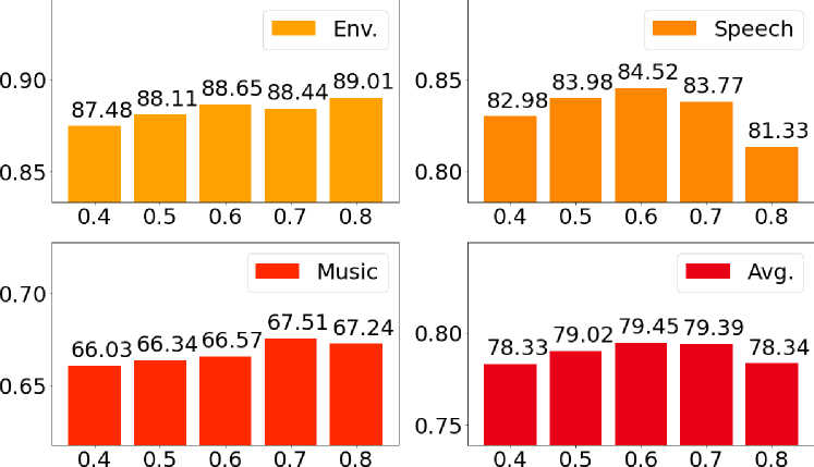
Fig. 3: Masking ratio ablations: linear evaluation results (%).

4.5 Comparison with SOTA

We compare the M2D with SOTA methods in this section. Linear evaluation results shown in Table 4 confirm that our method outperforms existing SSL methods in four tasks: UrbanSound8K, VoxCeleb1, CREMA-D, and GTZAN. Among them, M2D outperforms all previous methods with 87.6% on UrbanSound8K, 73.1% on VoxCeleb1, and 83.9% on GTZAN.

The fine-tuning results in Table 5 show that our method outperforms existing SSL methods on ESC-50 and Speech commands V2 tasks and gives the same SOTA result as ATST[22] on AudioSet20K. In particular, the result of 98.5% on Speech commands V2 outperforms all previous methods, including supervised learning. MSM-MAE[9] shows a new SOTA VoxCeleb1 result, and M2D with a masking ratio of 0.6 shows a comparable result.

While the M2D showed SOTA performance on many tasks, it underperforms supervised learning methods (EAT[24], PaSST[25], and HTS-AT[26]) on ESC-50 and speech models (Wav2Vec2[14], BigSSL[16], and BYOL-S[21]) on the speech tasks, suggesting a future research direction. In summary, the experiments demonstrate the effectiveness of M2D among SOTA methods.

5 Conclusion

In this study, we proposed a new method, Masked Modeling Duo (M2D), to learn representations directly by predicting masked patch representations using two networks. Unlike previous methods, we encode training signal representations using only masked patches rather than all input patches. We made the M2D so that it encourages both online and target networks to model the entire input in visible and masked patch representations, respectively, achieving an effective representation. To evaluate our method, we applied it to masked spectrogram modeling to learn general-purpose audio representations with an audio spectrogram as input. We evaluated the performance of our method on a variety of downstream tasks. Experiments validated the effectiveness of our method, and M2D showed state-of-the-art results on UrbanSound8K, VoxCeleb1, CREMA-D, and GTZAN in linear evaluation, and on AudioSet20K, ESC-50, and Speech commands V2 in fine-tuning. Our code is available online.

NOTE: The following appendix will not be on the ICASSP paper. Please cite the arXiv version if you reference the appendix of this paper.

Appendix A Experiments with Images

We validate the effectiveness of our M2D for images by conducting evaluations on ImageNet[41]. We pre-trained on ImageNet-1K[41], followed by fine-tuning. We report top-1 validation accuracy for a single crop image of $224\times 224$ same as in the MAE[1].

We used the MAE code as a base, as in Section 4 using audio, and made minimal changes to it, allowing comparison of differences only in the experimental subjects of interest. We also used ViT-Base[27] for the backbone. For pre-training, we set the number of epochs as 300 and the batch size as 2048. All other settings were the same as in the MAE, including the masking ratio of 0.75. The EMA decay rate $\tau$ for the target network update was also the same as in Section 4, linearly interpolated from 0.99995 at the start of training to 0.99999 at the end. For fine-tuning, we used the same source code and parameters as in the MAE.

We compare three models, MAE, M2D, and an M2D variant, that feed all patches to the target encoder. Table 6 shows the results. The results show the performance of the M2D variant with all patches input to the target, which is conventional, is comparable to MAE, and our M2D outperforms these methods, validating that our method is also effective on images in addition to audios.

Table 6: Fine-tuning results on ImageNet-1K.

Model	Target	Target	Top-1
	encoder	input	acc(%)
MAE		-	83.22 $\pm$ 0.024
M2D variant (conventional)	✓	All patches	83.22 $\pm$ 0.085
M2D (ours)	✓	Masked patches only	83.35 $\pm$ 0.211

References

- [1] K. He, X. Chen, S. Xie, Y. Li, P. Dollár, and R. Girshick, “Masked autoencoders are scalable vision learners,” in CVPR, 2022.
- [2] C. Tao, X. Zhu, G. Huang, Y. Qiao, X. Wang, and J. Dai, “Siamese image modeling for self-supervised vision representation learning,” arXiv preprint arXiv:2206.01204, 2022.
- [3] M. Assran, M. Caron, I. Misra, P. Bojanowski, F. Bordes, P. Vincent, A. Joulin, M. Rabbat, and N. Ballas, “Masked siamese networks for label-efficient learning,” in ECCV, 2022.
- [4] X. Chen, M. Ding, X. Wang, Y. Xin, S. Mo, Y. Wang, S. Han, P. Luo, G. Zeng, and J. Wang, “Context autoencoder for self-supervised representation learning,” arXiv preprint arXiv:2202.03026, 2022.
- [5] A. El-Nouby, G. Izacard, H. Touvron, I. Laptev, H. Jegou, and E. Grave, “Are large-scale datasets necessary for self-supervised pre-training?,” arXiv preprint arXiv:2112.10740, 2021.
- [6] P.-Y. Huang, H. Xu, J. Li, A. Baevski, M. Auli, W. Galuba, F. Metze, and C. Feichtenhofer, “Masked autoencoders that listen,” in NeurIPS, 2022.
- [7] A. Baade, P. Peng, and D. Harwath, “MAE-AST: Masked Autoencoding Audio Spectrogram Transformer,” in Interspeech, 2022, pp. 2438–2442.
- [8] D. Chong, H. Wang, P. Zhou, and Q. Zeng, “Masked spectrogram prediction for self-supervised audio pre-training,” arXiv preprint arXiv:2204.12768, 2022.
- [9] D. Niizumi, D. Takeuchi, Y. Ohishi, N. Harada, and K. Kashino, “Masked Spectrogram Modeling using Masked Autoencoders for Learning General-purpose Audio Representation,” in HEAR: Holistic Evaluation of Audio Representations (NeurIPS 2021 Competition), 2022, vol. 166, pp. 1–24.
- [10] A. Baevski, W.-N. Hsu, Q. Xu, A. Babu, J. Gu, and M. Auli, “data2vec: A general framework for self-supervised learning in speech, vision and language,” in ICML, 2022, pp. 1298–1312.
- [11] X. Chen and K. He, “Exploring simple siamese representation learning,” in CVPR, Jun 2021.
- [12] J.-B. Grill, F. Strub, F. Altché, C. Tallec, P. H. Richemond, E. Buchatskaya, C. Doersch, B. A. Pires, Z. D. Guo, M. G. Azar, B. Piot, K. Kavukcuoglu, R. Munos, and M. Valko, “Bootstrap your own latent - a new approach to self-supervised learning,” in NeurIPS, 2020.
- [13] A. T. Liu, S.-w. Yang, P.-H. Chi, P.-c. Hsu, and H.-y. Lee, “Mockingjay: Unsupervised speech representation learning with deep bidirectional transformer encoders,” in ICASSP, 2020, pp. 6419–6423.
- [14] A. Baevski, Y. Zhou, A. Mohamed, and M. Auli, “wav2vec 2.0: A framework for self-supervised learning of speech representations,” in NeurIPS, 2020.
- [15] W.-N. Hsu, B. Bolte, Y.-H. H. Tsai, K. Lakhotia, R. Salakhutdinov, and A. Mohamed, “HuBERT: Self-supervised speech representation learning by masked prediction of hidden units,” IEEE/ACM Trans. Audio, Speech, Language Process., p. 3451â3460, 2021.
- [16] Y. Zhang, D. S. Park, W. Han, J. Qin, A. Gulati, J. Shor, A. Jansen, Y. Xu, Y. Huang, S. Wang, et al., “BigSSL: Exploring the frontier of large-scale semi-supervised learning for automatic speech recognition,” IEEE J. Sel. Top. Signal Process., vol. 16, no. 6, pp. 1519â1532, 2022.
- [17] Y. Gong, C.-I. Lai, Y.-A. Chung, and J. Glass, “SSAST: Self-supervised audio spectrogram transformer,” in AAAI, 2022, vol. 36, pp. 10699–10709.
- [18] L. Wang, P. Luc, Y. Wu, A. Recasens, L. Smaira, A. Brock, A. Jaegle, J.-B. Alayrac, S. Dieleman, J. Carreira, and A. van den Oord, “Towards learning universal audio representations,” in ICASSP, 2022, pp. 4593–4597.
- [19] S. Ghosh, A. Seth, and S. Umesh, “Decorrelating feature spaces for learning general-purpose audio representations,” IEEE J. Sel. Topics Signal Process., vol. 16, no. 6, pp. 1402–1414, 2022.
- [20] D. Niizumi, D. Takeuchi, Y. Ohishi, N. Harada, and K. Kashino, “BYOL for Audio: Exploring pre-trained general-purpose audio representations,” IEEE/ACM Trans. Audio, Speech, Language Process., vol. 31, pp. 137â151, 2023.
- [21] N. Scheidwasser-Clow, M. Kegler, P. Beckmann, and M. Cernak, “SERAB: A multi-lingual benchmark for speech emotion recognition,” in ICASSP, 2022, pp. 7697–7701.
- [22] X. LI and X. Li, “ATST: Audio Representation Learning with Teacher-Student Transformer,” in Interspeech, 2022, pp. 4172–4176.
- [23] Y. Gong, Y.-A. Chung, and J. Glass, “AST: Audio spectrogram transformer,” in Interspeech, 2021, pp. 571–575.
- [24] A. Gazneli, G. Zimerman, T. Ridnik, G. Sharir, and A. Noy, “End-to-end audio strikes back: Boosting augmentations towards an efficient audio classification network,” arXiv preprint arXiv:2204.11479, 2022.
- [25] K. Koutini, J. Schlüter, H. Eghbal-zadeh, and G. Widmer, “Efficient training of audio transformers with patchout,” in Interspeech, 2022, pp. 2753–2757.
- [26] K. Chen, X. Du, B. Zhu, Z. Ma, T. Berg-Kirkpatrick, and S. Dubnov, “HTS-AT: A hierarchical token-semantic audio transformer for sound classification and detection,” in ICASSP, 2022, pp. 646–650.
- [27] A. Dosovitskiy, L. Beyer, A. Kolesnikov, D. Weissenborn, X. Zhai, T. Unterthiner, M. Dehghani, M. Minderer, G. Heigold, S. Gelly, J. Uszkoreit, and N. Houlsby, “An image is worth 16x16 words: Transformers for image recognition at scale,” in ICLR, 2021.
- [28] J. F. Gemmeke, D. P. W. Ellis, D. Freedman, A. Jansen, W. Lawrence, R. C. Moore, M. Plakal, and M. Ritter, “Audio Set: An ontology and human-labeled dataset for audio events,” in ICASSP, 2017, pp. 776–780.
- [29] K. J. Piczak, “ESC: Dataset for Environmental Sound Classification,” in ACM-MM, 2015, pp. 1015–1018.
- [30] J. Salamon, C. Jacoby, and J. P. Bello, “A dataset and taxonomy for urban sound research,” in ACM-MM, 2014, pp. 1041–1044.
- [31] P. Warden, “Speech Commands: A Dataset for Limited-Vocabulary Speech Recognition,” arXiv preprint arXiv::1804.03209, Apr. 2018.
- [32] A. Nagrani, J. S. Chung, and A. Zisserman, “Voxceleb: A large-scale speaker identification dataset,” in Interspeech, 2017, pp. 2616–2620.
- [33] K. MacLean, “Voxforge”, 2018, Available at http://www.voxforge.org/home.
- [34] H. Cao, D. G. Cooper, M. K. Keutmann, R. C. Gur, A. Nenkova, and R. Verma, “CREMA-D: Crowd-sourced emotional multimodal actors dataset,” IEEE Trans. Affective Comput., vol. 5, no. 4, 2014.
- [35] G. Tzanetakis and P. Cook, “Musical genre classification of audio signals,” IEEE Speech Audio Process., vol. 10, no. 5, 2002.
- [36] J. Engel, C. Resnick, A. Roberts, S. Dieleman, M. Norouzi, D. Eck, and K. Simonyan, “Neural audio synthesis of musical notes with WaveNet autoencoders,” in ICML, 2017.
- [37] J. Turian, J. Shier, G. Tzanetakis, K. McNally, and M. Henry, “One billion audio sounds from GPU-enabled modular synthesis,” in DAFx2020, 2021.
- [38] I. Loshchilov and F. Hutter, “SGDR: Stochastic gradient descent with warm restarts,” in ICLR, 2017.
- [39] H. Zhang, M. Cisse, Y. N. Dauphin, and D. Lopez-Paz, “mixup: Beyond empirical risk minimization,” in ICLR, 2018.
- [40] D. Niizumi, D. Takeuchi, Y. Ohishi, N. Harada, and K. Kashino, “Composing general audio representation by fusing multilayer features of a pre-trained model,” in EUSIPCO, 2022, pp. 200–204.
- [41] J. Deng, W. Dong, R. Socher, L.-J. Li, K. Li, and L. Fei-Fei, “Imagenet: A large-scale hierarchical image database,” in CVPR, 2009.