Generic Properties of First Order
Mean Field Games

Abstract

We consider a class of deterministic mean field games, where the state associated with each player evolves according to an ODE which is linear w.r.t. the control. Existence, uniqueness, and stability of solutions are studied from the point of view of generic theory. Within a suitable topological space of dynamics and cost functionals, we prove that, for “nearly all” mean field games (in the Baire category sense) the best reply map is single valued for a.e. player. As a consequence, the mean field game admits a strong (not randomized) solution. Examples are given of open sets of games admitting a single solution, and other open sets admitting multiple solutions. Further examples show the existence of an open set of MFG having a unique solution which is asymptotically stable w.r.t. the best reply map, and another open set of MFG having a unique solution which is unstable. We conclude with an example of a MFG with terminal constraints which does not have any solution, not even in the mild sense with randomized strategies.

1 Introduction

This paper deals with a class of mean field games with a continuum of players, where the state associated with each player evolves according to a controlled ODE. We study the existence, uniqueness, and stability of solutions from the point of view of generic theory. Namely, we seek properties of solutions that are satisfied either on some open set of MFG, or for “nearly all” MFG in the topological sense [12, 20]; i.e., for all MFG in the intersection of countably many open dense sets.

Let $(\Omega,{\cal B},\mu)$ be a probability space. More precisely, we assume that $\Omega$ is a metric space with Borel $\sigma$-algebra ${\cal B}$, while $\mu$ is an atomless probability measure on $\Omega$. Without loss of generality, throughout the following we assume $\Omega=[0,1]$ with Lebesgue measure. We regard $\xi\in\Omega$ as a Lagrangian variable, labelling one particular player. Accordingly, we shall denote by $t\mapsto x(t,\xi)$ a trajectory for player $\xi$. By selecting one trajectory $x(\cdot,\xi)\in{\cal C}\bigl{(}[0,T];\,I\!\!R^{n}\bigr{)}$ for each player (depending measurably on $\xi$), one obtains an element $X$ in the space

$${\bf L}^{1}\Big{(}\Omega\,;~{}{\cal C}\bigl{(}[0,T];\,I\!\!R^{n}\bigr{)}\Big{)}.$$ (1.1)

The space (1.1) is naturally endowed with the Banach norm

$$\|X\|~{}\doteq~{}\int_{\Omega}\left(\sup_{t\in[0,T]}\bigl{|}x(t,\xi)\bigr{|}\right)\,d\xi.$$ (1.2)

To define a (deterministic) mean field game, for each player $\xi\in\Omega$ we consider an optimal control problem where the dynamics and the cost functions also depend on the cumulative distribution $X$ of all other players. To express this dependence, we consider a finite number of smooth scalar functions $\phi_{1},\ldots,\phi_{N}\in{\cal C}^{2}\bigl{(}[0,T]\times I\!\!R^{n}\bigr{)}$, and define $\eta(t)=(\eta_{1},\ldots,\eta_{N})(t)$ to be the vector of “moments”

$$\eta_{i}(t)~{}=~{}\int_{\Omega}\phi_{i}\bigl{(}t,x(t,\xi)\bigr{)}\,d\xi,\qquad i=1,\ldots,N.$$ (1.3)

The control problem for player $\xi$ takes the form

$$\hbox{minimize:}\qquad\int_{0}^{T}L\bigl{(}t,x(t),u(t),\eta(t)\bigr{)}\,dt+\psi\bigl{(}x(T)\bigr{)},$$ (1.4)

subject to the dynamics

$$\dot{x}(t)~{}=~{}f\bigl{(}t,x(t),u(t),\eta(t)\bigr{)}\qquad\qquad t\in[0,T],$$ (1.5)

and with initial datum

$$x(\xi,0)\,=\,\bar{x}(\xi).$$ (1.6)

Definition 1.1

In the above setting, by a strong solution to the mean field game we mean a family of control functions $t\mapsto u(t,\xi)\in I\!\!R^{m}$ and corresponding trajectories $t\mapsto x(t,\xi)\in I\!\!R^{n}$, defined for $\xi\in\Omega$ and $t\in[0,T]$, such that the following holds.

For a.e. $\xi\in\Omega$, the control $u(\cdot,\xi)$ and the trajectory $x(\cdot,\xi)$ provide an optimal solution to the optimal control problem (1.4)–(1.6) for player $\xi$, where $\eta(t)=(\eta_{1},\ldots,\eta_{N})(t)$ is the vector of moments defined at (1.3).

A mean field game thus yields a (possibly multivalued) map $\eta\mapsto\Phi(\eta)$ from ${\cal C}([0,T];\,I\!\!R^{N})$ into itself. Namely, given $\eta(\cdot)$, for each $\xi\in\Omega$ consider an optimal trajectory $x^{\eta}(\cdot,\xi)$ of the corresponding optimal control problem (1.4)–(1.6). We then set

$$\Phi(\eta)~{}\doteq~{}\widetilde{\eta}~{}=~{}(\widetilde{\eta}_{1},\ldots,\widetilde{\eta}_{N}),\qquad\qquad\widetilde{\eta}_{i}(t)~{}\doteq~{}\int_{\Omega}\phi_{i}\bigl{(}t,x^{\eta}(t,\xi)\bigr{)}\,d\xi,$$ (1.7)

under suitable assumptions that will ensure that the integral in (1.7) is well defined. By definition, a fixed point of this composed map

$$\begin{array}[]{c}\qquad\eta(\cdot)\quad\mapsto\qquad\bigl{\{}x^{\eta}(\cdot,\xi)\,;~{}\xi\in\Omega\bigr{\}}\quad\mapsto\quad\widetilde{\eta}~{}=~{}\Phi(\eta)\\[5.69054pt] [\hbox{moments}]~{}\mapsto~{}[\hbox{optimal trajectories}]~{}\mapsto~{}[\hbox{moments}]\end{array}$$ (1.8)

yields a strong solution to the mean field game.

Remark 1.1

In general, the map $\Phi$ can be multivalued. Indeed, for some $\eta(\cdot)$, there can be a subset $V\subseteq\Omega$ with positive measure, such that each player $\xi\in V$ has two or more optimal trajectories. For this reason, a mean field game may not have a solution in the strong sense considered in Definition 1.1. In order to achieve a general existence theorem one needs to relax the concept of solution, allowing the possibility of randomized strategies [1, 6, 9]. This leads to the problem of finding a fixed point of an upper semicontinuous convex-valued multifunction, which exists by Kakutani’s theorem [10, 17].

Following the standard literature on fixed points of continuous or multivalued maps, we introduce

Definition 1.2

A solution $x=x^{*}(t,\xi)$ to the above mean field game is stable if the corresponding function $\eta^{*}\in{\cal C}^{0}\bigl{(}[0,T];\,I\!\!R^{N}\bigr{)}$ at (1.3) is a stable fixed point of the multifunction $\Phi$ at (1.7). Namely, for every $\varepsilon>0$ there exists $\delta>0$ such that the following holds. For every sequence $\bigl{(}\eta^{(k)}\bigr{)}_{k\geq 0}$ such that

$$\|\eta^{(0)}-\eta^{*}\|_{{\cal C}^{0}}~{}<~{}\delta,\qquad\quad\eta^{(k)}~{}\in~{}\Phi\bigl{(}\eta^{(k-1)}\bigr{)}\quad\hbox{for all}~{}k\geq 1,$$ (1.9)

one has $\|\eta^{(k)}-\eta^{*}\|_{{\cal C}^{0}}<\varepsilon$ for all $k\geq 1$.

If, in addition, every such sequence $\bigl{(}\eta^{(k)}\bigr{)}$ converges to $\eta^{*}$, then we say that the solution is asymptotically stable.

If the solution is not stable, we say that it is unstable.

Next, we say that a solution of the mean field game is structurally stable if it persists under small perturbations of the dynamics and the cost functionals. More precisely:

Definition 1.3

We say that a solution $x=x(t,\xi)$ to the above mean field game (1.3–(1.6) is structurally stable (or equivalently: essential) if, given $\varepsilon>0$, there exists $\delta>0$ such that the following holds. For any perturbations $(f^{\dagger},L^{\dagger},\psi^{\dagger},\phi^{\dagger},\bar{x}^{\dagger})$ satisfying

$$\max\Big{\{}\|f^{\dagger}-f\|_{{\cal C}^{2}}\,,~{}\|L^{\dagger}-L\|_{{\cal C}^{2}}\,,~{}\|\psi^{\dagger}-\psi\|_{{\cal C}^{2}}\,,~{}\|\phi^{\dagger}-\phi\|_{{\cal C}^{2}}\Big{\}}~{}<~{}\delta,\qquad\|\bar{x}^{\dagger}-\bar{x}\|_{{\bf L}^{\infty}}<\delta,$$ (1.10)

the corresponding perturbed game has a solution $x^{\dagger}=x^{\dagger}(t,\xi)$ such that

$$\sup_{t\in[0,T]}\int_{\Omega}\bigl{|}x^{\dagger}(t,\xi)-x(t,\xi)\bigr{|}\,d\xi~{}<~{}\varepsilon.$$ (1.11)

Throughout the following, we shall assume that the dynamics is affine w.r.t. the control variable:

$$f(x,u,\eta)~{}=~{}f_{0}(x,\eta)+\sum_{i=1}^{m}f_{i}(x,\eta)u_{i}\,,$$ (1.12)

and all functions $f,\psi,L$ have at least ${\cal C}^{2}$ regularity.

Since our MFG at (1.3)–(1.6) is characterized by the 5-tuple of functions $(f,L,\psi,\phi,\bar{x})$, we are interested in properties which are satisfied either (i) for all games where $(f,L,\psi,\phi,\bar{x})$ ranges inside an open set (in a suitable Banach space), or (ii) for generic games, i.e., for all games where $(f,L,\psi,\phi,\bar{x})$ ranges over the intersection of countably many open dense sets. Roughly speaking, the main results of the paper can be summarized as follows.

• Given a triple $(f,L,\phi)\in{\cal C}^{3}\times{\cal C}^{3}\times{\cal C}^{3}$, for a generic pair $(\psi,\bar{x})\in{\cal C}^{3}\times{\bf L}^{\infty}$, the best reply map $\eta\mapsto\Phi(\eta)$ in (1.8) is single valued. As a consequence, the MFG (1.3)–(1.6) admits a strong solution.

• There is an open set of mean field games with a unique solution, which is stable and essential.

• There is an open set of mean field games with a unique solution, which is unstable, and essential.

• There is an open set of mean field games with two solutions, both essential.

More precise statements of these results will be given in the following sections. The remainder of the paper is organized as follows.

As a warm-up, in Section 2 we review the basic tools for proving generic properties. Here we consider a family of optimal control problems where the dynamics is linear w.r.t. the control functions. We show that, for generic dynamics $f$, running cost $L$ and terminal cost $\psi$, for a.e. initial datum $x(0)=\overline{x}$ the optimal control is unique.

Section 3 provides a simple way to construct mean field games with multiple solutions. Given an optimal control problem and a pair $(x^{*},u^{*})$ (not necessarily optimal) which satisfies the Pontryagin necessary conditions, we show the existence of a mean field game where $u^{*}$ is the optimal control for every player. As a consequence, for any control problem where the Pontryagin equations have multiple solutions, one can construct a MFG with multiple solutions. Under generic assumptions, all of these solutions are structurally stable.

Section 4 contains the main result of the paper. Namely, for a generic MFG of the form (1.3)–(1.6), the best reply map $\eta\mapsto\Phi(\eta)$ is single valued. Hence the MFG admits a strong solution. Here the analysis is far more delicate than in the proof of the generic uniqueness for the optimal control problem in Section 2. Indeed, we need to show that the statement

• The set of initial points $\overline{x}$, for which the problem (1.4)–(1.6) has multiple solutions, has measure zero

is true not just for one function $\eta(\cdot)$, but simultaneously for all functions $\eta=(\eta_{1},\ldots,\eta_{N})$, in a suitable domain.

Finally, Section 5 collects a variety of examples, where the MFG have multiple strong solutions, Some of these are stable, in the sense of Definition 1.2, while others are unstable.

We conclude with two examples of MFG without solution. The first one is a well known case where nonexistence is due to the fact that the best reply of each player is not unique. No strong solution exists, but one can construct a mild solution where each player adopts a randomized strategy. In the second example, the presence of a terminal constraint lacking a transversality condition prevents the existence of any solution, even in the mild (randomized) sense.

Some concluding remarks, pointing to future research directions, are given in Section 6.

Mean field games with stochastic dynamics have been introduced by Lasry and Lions [18] and by Huang, Malhamé and Caine [16], to model the behavior of a large number of interacting agents. Their solution leads to a well known system of forward-backward parabolic equations. Solutions to first order MFG (with deterministic dynamics) can be obtained as a vanishing viscosity limit of these parabolic PDEs, i.e., as viscosity solutions to a corresponding Hamilton-Jacobi equation [6, 7, 8, 9]. Equivalently, one can take a Lagrangian approach, describing the optimal control and the optimal trajectory of each single agent. This is the approach followed in the present paper. Some examples of MFG with unique or with multiple solutions can be found in [1]. A concept of structural stability for solutions to first order MFG was proposed in [5].

2 Generic uniqueness for optimal control problems

Consider an optimal control problem of the form

$$\hbox{minimize:}\qquad J[u]~{}\doteq~{}\displaystyle\int_{0}^{T}L\bigl{(}x(t),u(t)\bigr{)}\,dt+\psi\bigl{(}x(T)\bigr{)},$$ (2.1)

with dynamics which is affine in the control:

$$\dot{x}(t)~{}=~{}f\bigl{(}x(t),u(t)\bigr{)}~{}=~{}f_{0}(x(t))+\sum_{i=1}^{m}f_{i}(x(t))\,u_{i}(t),\qquad\quad x(0)=\bar{x}.$$ (2.2)

Here $u(t)\in I\!\!R^{m}$ while $x(t)\in I\!\!R^{n}$. To fix ideas, we shall consider the couple $(f,L)$ satisfying the following assumptions.

• The functions $f_{i}:I\!\!R^{n}\mapsto I\!\!R^{n}$, $i=0,\ldots,m$, are twice continuously differentiable. Moreover the vector fields $f_{i}$ satisfy the sublinear growth condition

  $$\bigl{|}f_{i}(x)\bigr{|}~{}\leq~{}c_{1}\,\bigl{(}|x|+1\bigr{)}$$ (2.3)

  for some constant $c_{1}>0$ and all $x\in I\!\!R^{n}$.

• The running cost $L:I\!\!R^{n}\times I\!\!R^{m}\mapsto I\!\!R$ is twice continuously differentiable and satisfies

  $$\left\{\begin{array}[]{rl}L(x,u)&\geq~{}c_{2}\bigl{(}|u|^{2}-1\bigr{)},\\[5.69054pt] |L_{x}(x,u)|&\leq~{}\ell(|x|)\cdot(1+|u|^{2}),\end{array}\right.$$ (2.4)

  for some constant $c_{2}>0$ and some continuous function $\ell$. Moreover, $L$ is uniformly convex w.r.t. $u$. Namely, for some $\delta_{L}>0$, the $m\times m$ matrix of second derivatives w.r.t. $u$ satisfies

  $$L_{uu}(x,u)~{}>~{}\delta_{L}\cdot\mathbb{I}_{m}\qquad\qquad\hbox{for all}~{}x,u.$$ (2.5)

  Here $\mathbb{I}_{m}$ denotes the $m\times m$ identity matrix

Throughout the following, the open ball centered at the origin with radius $r$ is denoted by $B_{r}=B(0,r)$, while $\overline{B}_{r}$ denotes its closure. Under the previous assumptions, optimal controls and optimal trajectories of the optimization problem (2.1)-(2.2) satisfy uniform a priori bounds:

Lemma 2.1

Assume that the couple $(f,L)$ satisfies (A1)-(A2) and $\psi:I\!\!R^{n}\to[0,\infty[$ is twice continuously differentiable. Then there exist continuous functions $\alpha,\beta:[0,\infty[\to[0,\infty[$ such that the following holds. Given any initial point $\bar{x}\in\overline{B}_{r}$, let $u^{*}(\cdot)$ be an optimal control and let $x^{*}(\cdot)$ be the corresponding optimal trajectory and for the problem (2.1)-(2.2). Then

$$\hbox{\rm ess-}\!\!\!\sup_{t\in[0,T]}|u^{*}(t)|~{}\leq~{}\alpha(r),\qquad\qquad\sup_{t\in[0,T]}|x^{*}(t)|~{}\leq~{}\beta(r).$$ (2.6)

Proof. Fix $\bar{x}\in\overline{B}_{r}$. Calling $x_{0}(\cdot)$ the solution of (2.2) with $u(t)\equiv 0$, by (2.3) it follows

$$\sup_{t\in[0,T]}|x_{0}(t)|~{}\leq~{}(r+1)\cdot e^{c_{1}t}-1.$$

Let $(x^{*},u^{*})$ be a pair of optimal trajectory and optimal control of the optimization problem (2.1)-(2.2). By the first inequality in (2.4), one has

$$\int_{0}^{T}\big{|}u^{*}(t)|^{2}dt~{}\leq~{}{1\over c_{2}}\,\left(\int_{0}^{T}L(x_{0}(t),0)dt+\psi(x_{0}(T))\right)+T\\ ~{}=~{}{1\over c_{2}}\cdot\left(T\cdot\sup_{|y|\leq(r+1)\cdot e^{c_{1}T}-1}L(y,0)+\sup_{|y|\leq(r+1)\cdot e^{c_{1}T}-1}|\psi(y)|\right)+T~{}\doteq~{}\beta_{1}(r).$$ (2.7)

Since $x^{*}$ solves (2.2) with $u\equiv u^{*}$, we have

$$|\dot{x}(t)|~{}\leq~{}c_{1}\cdot(|x|+1)\cdot\left(1+\sum_{i=1}^{m}|u^{*}_{i}(t)|\right)~{}\leq~{}{c_{1}\over 2}\cdot\bigl{(}|x|+1\bigr{)}\bigl{(}|u^{*}(t)|^{2}+m+2\bigr{)}.$$

Therefore, from (2.7) one obtains

$$\sup_{t\in[0,T]}|x^{*}(t)|~{}\leq~{}(r+1)\cdot\exp\left({c_{1}\over 2}\cdot[\beta_{1}(r)+(m+2)T]\right)-1~{}\doteq~{}\beta(r).$$

To derive a pointwise bound on $u^{*}$, for every $\alpha\geq 0$ we consider the truncated function

$$u_{\alpha}(s)~{}=~{}\begin{cases}u^{*}(s)&\mathrm{if}\qquad|u^{*}(s)|\leq\alpha,\\ 0&\mathrm{if}\qquad|u^{*}(s)|>\alpha.\end{cases}$$

Calling $x_{\alpha}$ the solution of (2.2) with $u\equiv u_{\alpha}$, we have

$$\sup_{t\in[0,T]}|x_{\alpha}(t)|~{}\leq~{}\beta(r),\qquad\sup_{t\in[0,T]}|x^{*}(t)-x_{\alpha}(t)|~{}\leq~{}\beta_{2}(r)\cdot\int_{I_{\alpha}}|u^{*}(s)|ds$$

for some continuous function $\beta_{2}$. For any constant $\gamma\geq 1$, setting $I_{\gamma}\doteq\bigl{\{}s\in[0,T]:|u^{*}(s)|>\gamma\bigr{\}}$ we estimate the difference in the costs:

$$\begin{array}[]{l}\displaystyle 0~{}\leq~{}J[u_{\gamma}]-J[u^{*}]~{}=~{}\int_{0}^{T}L(x_{\gamma}(t),u_{\gamma}(t))-L(x^{*}(t),u^{*}(t))dt+\psi(x_{\gamma}(T))-\psi(x_{*}(T))\\[11.38109pt] \qquad\displaystyle~{}\leq~{}\left((T+\beta_{1}(r))\cdot\sup_{|s|\leq\beta(r)}\ell(s)+\sup_{|y|\leq\beta(r)}|\nabla\psi(y)|\right)\cdot\beta_{2}(r)\cdot\int_{I_{\gamma}}|u^{*}(s)|ds\\[11.38109pt] \qquad\qquad\displaystyle+\int_{I_{\gamma}}L(x^{*}(t),0)-L(x^{*}(t),u^{*}(t))dt\\[11.38109pt] \qquad\displaystyle~{}\leq~{}\alpha_{1}(r)\cdot\int_{I_{\gamma}}|u^{*}(s)|ds-c_{2}\cdot\int_{I_{\alpha}}|u^{*}(s)|^{2}ds~{}\leq~{}\left(\alpha_{1}(r)-c_{2}\cdot\gamma\right)\end{array}$$

for some continuous function $\alpha_{1}(\cdot)$. This yields the first inequality in (2.6), with $\displaystyle\alpha(r)={\alpha_{1}(r)/c_{2}}$. MM     

In the following, the positive cone in the Banach space ${\cal C}^{2}$ is denoted by

$${\cal C}^{2}_{+}(I\!\!R^{n})~{}\doteq~{}\left\{\psi\in{\cal C}^{2}(I\!\!R^{n})\,;~{}\inf_{x\in I\!\!R^{n}}\psi(x)>0\right\}.$$ (2.8)

We can now state the first result.

Theorem 2.1

(Generic uniqueness for optimal control problems). Under the assumptions (A1)-(A2), there exists a ${\cal G}_{\delta}$ subset ${\cal M}\subset{\cal C}^{2}_{+}(I\!\!R^{n})$ such that the following holds. For every $\psi\in{\cal M}$, the set of initial points $\bar{x}\in I\!\!R^{n}$, for which the optimal control problem (2.1)-(2.2) has multiple solutions, has Lebesgue measure zero.

Proof. 1. For every $\psi\in{\cal C}^{2}_{+}(I\!\!R^{n})$ and any integer $\nu\geq 1$, we consider a set of initial points yielding two distinct solutions:

$$\begin{array}[]{rl}S_{\nu}(\psi)&\doteq~{}\Big{\{}\bar{x}\in\overline{B}_{\nu},~{}\hbox{the optimization problem (\ref{oc1})-(\ref{oc2}) has two solutions}\\[5.69054pt] &x_{1}(\cdot),~{}x_{2}(\cdot),\displaystyle\hbox{ with the same minimum cost, and with $\displaystyle\bigl{|}x_{1}(T)-x_{2}(T)\bigr{|}\geq{1\over\nu}$ }\Big{\}}.\end{array}$$ (2.9)

Next, consider the set of terminal cost $\psi$ leading to a small set of multiple solutions:

$${\cal M}_{\nu}~{}\doteq~{}\left\{\psi\in{\cal C}^{2}_{+}(I\!\!R^{n})\,;~{}~{}\hbox{meas}\bigl{(}S_{\nu}(\psi)\bigr{)}~{}<~{}{1\over\nu}\right\}.$$ (2.10)

The theorem will be proved by showing that ${\cal M}_{\nu}$ is open and dense in ${\cal C}^{2}_{+}(I\!\!R^{n})$. Indeed, if this is the case then the set ${\cal M}=\displaystyle\bigcap_{\nu\geq 1}{\cal M}_{\nu}$ is a ${\cal G}_{\delta}$ subset of ${\cal C}^{2}_{+}(I\!\!R^{n})$. Moreover, for any $\psi\in{\cal M}$, calling $S(\psi)$ the set of initial points $\bar{x}\in I\!\!R^{n}$ for which the optimization problem (2.1)-(2.2) has two optimal trajectories ending at distinct terminal points, we have

$$\hbox{meas}\big{(}S(\psi)\big{)}~{}\leq~{}\limsup_{\nu\to\infty}\big{[}\hbox{meas}\bigl{(}S_{\nu}(\psi)\bigr{)}\big{]}~{}=~{}0.$$ (2.11)

We now observe that, for every $\bar{x}\in I\!\!R^{n}$, the Pontryagin necessary conditions [4, 11, 13] take the form

$$\left\{\begin{array}[]{rl}\dot{x}&=~{}f\bigl{(}x,u(x,p)\bigr{)},\\[8.53581pt] \dot{p}&=~{}-p\cdot f_{x}\bigl{(}x,u(x,p)\bigr{)}-L_{x}(x,u(x,p)),\end{array}\right.$$ (2.12)

with boundary conditions

$$\left\{\begin{array}[]{rl}x(0)&=~{}\bar{x},\\[5.69054pt] p(T)&=~{}\nabla\psi\bigl{(}x(T)\bigr{)}.\end{array}\right.$$ (2.13)

Here the optimal control is determined as the pointwise minimizer

$$u(x,p)~{}=~{}\hbox{arg}\!\min_{\omega\in I\!\!R^{m}}\Big{\{}L(x,\omega)+p\,f(x,\omega)\Big{\}}.$$ (2.14)

By assumptions, $f$ is affine w.r.t. $\omega$, while by (2.5) the cost function $L$ is uniformly convex. As a consequence, the minimizer in (2.14) is unique. Therefore, the map $(x,p)\mapsto u(x,p)$ is well defined and continuously differentiable, and the system of ODEs (2.12) has ${\cal C}^{1}$ right hand sides. We conclude that, for any $y\in I\!\!R^{n}$, the system (2.12) with terminal conditions

$$x(T)~{}=~{}y,\qquad p(T)~{}=~{}\nabla\psi(y),$$ (2.15)

admits a unique solution $t\mapsto(x,p)(t;y)$ on $[0,T]$. In particular, this implies that if two optimal trajectories starting from $\bar{x}$ have the same terminal point, then then they must coincide for all $t\in[0,T]$. Hence (2.11) yields (ii).

2. Given $\nu\geq 1$, we now claim that ${\cal M}_{\nu}$ is open in ${\cal C}^{2}_{+}(I\!\!R^{n})$. Indeed, thanks to the uniform bounds on optimal controls and optimal trajectories proved in Lemma 2.6, standard arguments show that each set $S_{\nu}(\psi)$ is closed and bounded. Moreover, since the minimum cost for (2.1)-(2.2) depends continuously on $\bar{x},f,L,\psi$, the map $\psi\mapsto S_{\nu}(\psi)$ is upper semicontinuous.

Given any terminal cost $\widetilde{\psi}\in{\cal M}_{\nu}$, let $A$ be an open set such that

$$S_{\nu}(\widetilde{\psi})\,\subset\,A,\qquad\qquad\hbox{meas}(A)<{1\over\nu}\,.$$

Based on Lemma 2.1, for any initial datum $\bar{x}\in\overline{B}_{\nu}$, every optimal control $u^{*}$ and optimal trajectory $x^{*}$ satisfy

$$\hbox{\rm ess-}\!\!\!\sup_{t\in[0,T]}|u^{*}(t)|~{}\leq~{}\alpha(\nu),\qquad\qquad\sup_{t\in[0,T]}|x^{*}(t)|~{}\leq~{}\beta(\nu).$$ (2.16)

By upper semicontinuity, there exists $\delta_{0}>0$ such that

$$\|\psi-\widetilde{\psi}\|_{{\cal C}^{2}}~{}<~{}\delta_{0}\qquad\Longrightarrow\qquad S_{\nu}(\psi)\,\subset\,A,\qquad\inf_{x\in I\!\!R^{n}}\widetilde{\psi}>0.$$

As a consequence, $\psi\in{\cal M}_{\nu}$, proving our claim.

3. In the remaining steps, we prove that each ${\cal M}_{\nu}$ is dense in ${\cal C}^{2}_{+}(I\!\!R^{n})$. Given any $\psi\in{\cal C}^{2}_{+}(I\!\!R^{n})$, we shall construct a small perturbation of $\psi$ that lies inside ${\cal M}_{\nu}$.

Using Lemma 2.1, we choose a radius $\rho>0$ large enough so that the ball $B_{\rho}$ contains all trajectories that satisfy the PMP (2.12) and start at some point $\bar{x}\in\overline{B}_{\nu}$.

Denoting by $t\mapsto(x,p)(t;y)$ the unique solution of the system of ODEs (2.12) with terminal data (2.15), we observe that the map $y\mapsto x(0;y)$ is ${\cal C}^{1}$. Consider the sets

$$S_{\delta_{0}}~{}\doteq~{}\Big{\{}x(0,y)\,;~{}~{}y\in B_{\rho},\quad\bigl{|}\det(D_{y}x(0,y))\bigr{|}\leq\delta_{0}\Big{\}},\quad\qquad S^{-1}_{\delta_{0}}\,\doteq\,\big{\{}y\,;~{}x(0,y)\in S_{\delta_{0}}\big{\}}.$$ (2.17)

By choosing $\delta_{0}>0$ sufficiently small we obtain

$$\hbox{meas}\bigl{(}S_{\delta_{0}}\bigr{)}~{}\leq~{}\delta_{0}\cdot\hbox{meas}(B_{\rho})~{}<~{}{1\over 2\nu}.$$ (2.18)

Next, consider the open subset of couples in $I\!\!R^{n+n}$

$$\Gamma_{\nu}~{}\doteq~{}\left\{(y_{1},y_{2})\in\left(B_{\rho}\backslash S^{-1}_{\delta_{0}}\right)\times\left(B_{\rho}\backslash S^{-1}_{\delta_{0}}\right)\,;~{}~{}|y_{1}-y_{2}|>{9\over 10\nu}\right\}.$$ (2.19)

For every couple of points $(\bar{y}_{1},\bar{y}_{2})\in\Gamma_{\nu}$, let $\varphi^{(\bar{y}_{1},\bar{y}_{2})}\in{\cal C}^{\infty}_{c}(I\!\!R^{n})$ be a smooth function with compact support such that

$$\varphi^{(\bar{y}_{1},\bar{y}_{2})}(y)~{}=~{}\left\{\begin{array}[]{rl}1&\hbox{if}\quad|y-\bar{y}_{1}|\leq{1\over 5\nu},\\[8.53581pt] -1&\hbox{if}\quad|y-\bar{y}_{2}|\leq{1\over 5\nu},\\[8.53581pt] 0&\hbox{if}\quad|y-\bar{y}_{1}|\geq{2\over 5\nu}~{}~{}\hbox{and}~{}~{}|y-\bar{y}_{2}|\geq{2\over 5\nu}.\end{array}\right.$$ (2.20)

Covering the compact closure $\overline{\Gamma}_{\nu}$ with finitely many balls, say $B\left(\bigl{(}y^{k}_{1},y^{k}_{2}\bigr{)},{1\over 5\nu}\right)$ for $(y^{k}_{1},y^{k}_{2})\in\overline{\Gamma}_{\nu}$, $k\in\{1,\dots,N_{\nu}\}$, we define a family of terminal costs, depending on the additional parameters $\theta=\bigl{(}\theta_{1},\dots,\theta_{N_{\nu}}\bigr{)}$:

$$\psi^{\theta}(y)~{}=~{}\psi(y)+\sum_{k=1}^{N_{\nu}}\theta_{k}\cdot\varphi^{(y^{k}_{1},y^{k}_{2})}(y)\qquad\hbox{for all}~{}y\in I\!\!R^{n}.$$ (2.21)

4. For any given $\theta\in I\!\!R^{N_{\nu}}$, let $(x^{\theta}(s;y),p^{\theta}(s;y))$ be the solution of (2.12) with terminal condition $(x(T),p(T))=\big{(}y,\nabla\psi^{\theta}(y)\big{)}$. We denote by $J^{\theta}(y)$ the cost of this trajectory:

$$J^{\theta}(y)~{}=~{}\int_{0}^{T}L\big{(}x^{\theta}(t;y),u\big{(}x^{\theta}(t;y),p^{\theta}(t;y)\big{)}\big{)}dt+\psi^{\theta}(y).$$

Observe that, for any $k\in\{1,\dots,N_{\nu}\}$ and any $y\in B\left(y^{k}_{1},{1\over 5\nu}\right)\bigcup B\left(y^{k}_{2},{1\over 5\nu}\right)$, the definition (2.20) implies

$$\nabla\psi^{\theta}(y)~{}=~{}\nabla\psi(y)+\sum_{j\in\{1,\dots,N_{\nu}\}\backslash\{k\}}\theta_{j}\cdot\nabla\varphi^{(y^{j}_{1},y^{j}_{2})}(y).$$ (2.22)

In this case, $\left(x^{\theta}(t;y),p^{\theta}(t;y)\right)$ does not depend on $\theta_{k}$ and

$${\partial x^{\theta}\over\partial\theta_{k}}(0;y)~{}=~{}0,\qquad\quad{\partial J^{\theta}\over\partial\theta_{k}}(y)~{}=~{}{\partial\psi^{\theta}\over\partial\theta_{k}}(y)~{}=~{}\begin{cases}~{}1&\mathrm{if}\quad y\in B\left(y^{k}_{1},{1\over 5\nu}\right),\\[5.69054pt] -1&\mathrm{if}\quad y\in B\left(y^{k}_{2},{1\over 5\nu}\right).\end{cases}$$ (2.23)

5. Define the map $\Phi:\Gamma_{\nu}\times I\!\!R^{N_{\nu}}\to I\!\!R^{n+1}$ by setting

$$\Phi(y_{1},y_{2},\theta)~{}=~{}\left(x^{\theta}(0;y_{1})-x^{\theta}(0;y_{2}),J^{\theta}(y_{1})-J^{\theta}(y_{2})\right).$$ (2.24)

for all $(y_{1},y_{2},\theta)\in\Gamma_{\nu}\times I\!\!R^{N_{\nu}}$. For any $k\in\{1,2,\dots,N_{\nu}\}$, by (2.23) it now follows

$${\partial\Phi\over\partial\theta_{k}}(y_{1},y_{2},\theta)~{}=~{}(0,0,2)\qquad\hbox{for all}~{}(y_{1},y_{2})\in B\left(\big{(}y^{k}_{1},y^{k}_{2}\big{)},{1\over 5\nu}\right).$$

Moreover, by (2.17) and (2.21), there exists $\delta_{1}>0$ small enough such that

$$\Big{|}\mathrm{det}\bigl{(}D_{y}x^{\theta}(0;y_{i})\bigr{)}\Big{|}~{}>~{}{\delta_{0}\over 2},\qquad i\in\{1,2\},~{}~{}\theta=(\theta_{1},\ldots,\theta_{N_{\nu}})\in B_{\delta_{1}}.$$ (2.25)

Therefore, $\mathrm{rank}\Big{(}D\Phi(y_{1},y_{2},\theta)\Big{)}=n+1$ and $\Phi$ is transversal to the zero manifold

$$\{(0,0)\}~{}\subset~{}I\!\!R^{n}\times I\!\!R$$

on $B\left((y^{k}_{1},y^{k}_{2}),\,{1\over 5\nu}\right)\times B(0,\delta_{1})$. Since these balls provide a covering, we conclude that $\Phi$ is transversal to $\{(0,0)\}$ on the whole domain $\Gamma_{\nu}\times B(0,\delta_{1})$.

6. Finally, by the transversality theorem [3, 14], there exists a set $\Theta\subset I\!\!R^{N_{\nu}}$, dense in the ball $B(0,\delta_{1})$, such that for every $\theta\in\Theta$ the map $\Phi(\cdot,\cdot,\theta)$ is transversal to the zero manifold $\big{\{}(0,0)\}\subset I\!\!R^{n}\times I\!\!R$. This means: for every couple $(\bar{y}_{1},\bar{y}_{2})\in\Gamma_{\nu}$ such that

$$x^{\theta}(0,\bar{y}_{1})=x^{\theta}(0,\bar{y}_{2}),\qquad\quad J^{\theta}(\bar{y}_{1})=J^{\theta}(\bar{y}_{2}),$$

the Jacobian $D_{(y_{1},y_{2})}\Phi(\bar{y}_{1},\bar{y}_{2},\theta)$ has rank $n+1$. Hence, by the implicit function theorem, the set of couples

$$\Gamma_{(\bar{y}_{1},\bar{y}_{2})}(r)~{}\doteq~{}\Big{\{}(y_{1},y_{2})\in B\big{(}\big{(}\bar{y}_{1},\bar{y}_{2}\big{)},r\big{)}\cap\Gamma_{\nu}\,;~{}~{}\Phi(y_{1},y_{2},\theta)=(0,0)\in I\!\!R^{n+1}\Big{\}}$$

is contained in an $(n-1)$-dimensional manifold, for some $r>0$ small. The $n$-dimensional measure of this set is thus

$$\hbox{meas}\left(\bigl{\{}x^{\theta}(0;y_{1})\,;~{}~{}(y_{1},y_{2})\in\Gamma_{(\bar{y}_{1},\bar{y}_{2})}(r)\bigr{\}}\right)~{}=~{}0.$$

In turn, for every $\theta\in\Theta$ this implies

$$\hbox{meas}\Big{(}\bigl{\{}x^{\theta}(0;y_{1})\in I\!\!R^{n};~{}~{}\hbox{there exists $y_{2}\in I\!\!R^{n}$ such that}~{}~{}(y_{1},y_{2})\in\Gamma_{\nu},~{}\Phi(y_{1},y_{2},\theta)=0\bigr{\}}\Big{)}~{}=~{}0.$$

On the other hand, since there exists a constant $C>0$ such that

$$\big{|}x^{\theta}(0,y)-x(0,y)\big{|}~{}\leq~{}C|\theta|\qquad\hbox{for all}~{}\theta\in\Theta,~{}y\in S^{-1}_{\delta_{0}},$$

we have

$$\left\{x^{\theta}(0,y)\,;~{}~{}y\in S^{-1}_{\delta_{0}}\right\}~{}\subseteq~{}B\bigl{(}S_{\delta_{0}},\,C|\theta|\bigr{)}.$$ (2.26)

Since $S_{\delta_{0}}$ is compact, the measure of the $\varepsilon$-neighborhood around the set $S_{\delta_{0}}$ satisfies

$$\lim_{\varepsilon\to 0}~{}\hbox{meas}\Big{(}B(S_{\delta_{0}},\varepsilon)\Big{)}~{}=~{}\hbox{meas}(S_{\delta_{0}}).$$

Therefore, choosing $|\theta|$ small enough, by (2.18) and (2.26) we obtain

$$\begin{array}[]{l}\displaystyle\hbox{meas}\bigl{(}S_{\nu}(\psi^{\theta})\bigr{)}~{}\leq~{}\hbox{meas}\Big{(}\bigl{\{}x^{\theta}(0,y)\,;~{}~{}y\in S^{-1}_{\delta_{0}}\bigr{\}}\Big{)}\\[8.53581pt] \qquad\displaystyle~{}\leq~{}\hbox{meas}\left(B\bigl{(}S_{\delta_{0}},\,C|\theta|\bigr{)}\right)~{}<~{}\hbox{meas}\bigl{(}S_{\delta_{0}}\bigr{)}+{1\over 2\nu}~{}<~{}{1\over\nu}\,.\end{array}$$

Hence the terminal cost $\psi^{\theta}$ lies in ${\cal M}_{\nu}$. This shows that ${\cal M}_{\nu}$ is everywhere dense, completing the proof. MM     

3 Non-uniqueness for mean field games

Consider again the optimal control problem (2.1)-(2.2), with $f,L$ satisfying (A1)-(A2) and $\psi\in{\cal C}^{2}_{+}$. Let $Y^{*}(t)\doteq\begin{pmatrix}x^{*}(t)\cr p^{*}(t)\end{pmatrix}$ be a solution to Pontryagin’s optimality conditions (2.12)-(2.14). Linearizing the system of ODEs in (2.12) at $Y^{*}$, we obtain a system of the form

$$\dot{Y}~{}=~{}A(t)Y,$$ (3.1)

describing the evolution of a first order perturbation. We shall assume that $Y(t)=\begin{pmatrix}X(t)\cr P(t)\end{pmatrix}\equiv 0$ is the only solution to the linearized system (3.1) with boundary conditions

$$X(0)~{}=~{}0,\qquad\qquad P(T)~{}=~{}D^{2}\psi(x^{*}(T))\cdot X(T).$$ (3.2)

Notice that these assumptions imply that this solution is structurally stable. By the implicit function theorem, one can slightly perturb the dynamics and the cost function, and still find a solution to the equations (2.12)–(2.14) close to $Y^{*}$.

In this setting, it is easy to construct a MFG where $x(t,\xi)=x^{*}(t)$ is a structurally stable solution. Indeed, define the barycenter

$$b(t)~{}\doteq~{}\int_{0}^{1}x(t,\xi)\,d\xi.$$ (3.3)

Consider a game where the state of each player evolves with the same dynamics

$$\dot{x}(t)~{}=~{}f\bigl{(}x(t),u(t)\bigr{)}~{}=~{}f_{0}(x(t))+\sum_{i=1}^{m}f_{i}(x(t))\cdot u_{i}(t),\qquad x(\xi,0)=\bar{x},\qquad\xi\in[0,1],$$ (3.4)

and all players share the same cost functional

$$J~{}\doteq~{}\int_{0}^{T}\Big{[}L\bigl{(}x(t),u(t)\bigr{)}+\kappa\bigl{|}x(t)-b(t)\bigr{|}^{2}\Big{]}\,dt+\psi\bigl{(}x(T)\bigr{)}.$$ (3.5)

Theorem 3.1

Assume that $f,L$ satisfy (A1)-(A2) while $\psi\in{\cal C}^{2}_{+}$. Let $(x^{*},p^{*})$ be a solution to the Pontryagin equations (2.12)-(2.14). Then, if the constant $\kappa>0$ is large enough, the MFG (3.5)-(3.4) admits a solution where $x(t,\xi)=x^{*}(t)$ for all $\xi\in[0,1]$, $t\in[0,T]$.

If the linearized system (3.1)-(3.2) has only the zero solution, then this solution of the MFG is structurally stable.

Proof. 1. W.l.o.g., we can assume $\psi=0$. Indeed, the above optimal control problem can always be written as a Bolza problem, replacing the functional $J$ at (2.1) with

$$J^{\sharp}~{}\doteq~{}\int_{0}^{T}\bigl{[}L(x,u)+\nabla\psi(x)\cdot f(x,u)\bigr{]}\,dt.$$ (3.6)

If $\bigl{(}x(t),p(t),u(t)\bigr{)}$ provide a solution to the equations (2.12)-(2.14) for the original problem, one readily checks that the triple $\bigl{(}x(t),p(t)-\nabla\psi(x(t)),u(t)\bigr{)}$ provides a solution to the corresponding Pontryagin’s equations for the Bolza problem (3.6). 2. We thus assume that $\psi=0$. For every given $b\in{\cal C}^{0}([0,T])$ with $\|b-b^{*}\|_{{\cal C}^{0}}\leq 1$, we claim that (3.4)-(3.5) admits a unique optimal solution for $\kappa>0$ sufficiently large. Indeed, let $(u^{b},x^{b})$ be a pair of optimal control and optimal trajectory of (3.4)-(3.5). By Lemma 2.6, it follows

$$\|u^{b}\|_{{\bf L}^{\infty}},\|x^{b}\|_{{\cal C}^{0}}~{}\leq~{}C_{1},\qquad\kappa\cdot\int_{0}^{T}|x^{b}(t)-b(t)|^{2}dt~{}\leq~{}C_{1},$$ (3.7)

for some $C_{1}>0$ which depends only on $f,L$ and $T$. By the necessary conditions, there exists $p^{b}\in C^{0}([0,T])$ such that $(x^{b},p^{b},u^{b})$ solves the PMP

$$\left\{\begin{array}[]{rl}\dot{x}&=~{}f\bigl{(}x,u(x,p)\bigr{)},\\[8.53581pt] \dot{p}&=~{}-p\cdot f_{x}\bigl{(}x,u(x,p)\bigr{)}-L_{x}(x,u(x,p))-2\kappa(x-b)\,,\end{array}\right.$$ (3.8)

with $x(0)=\bar{x}$, $p(T)=0$ and, recalling (2.14),

$$u^{b}(t)~{}=~{}u\bigl{(}x^{b}(t),p^{b}(t)\bigr{)},~{}\qquad t\in[0,T].$$

By (3.7) and the second equation of (3.8) we deduce

$$\|p^{b}\|_{{\cal C}^{0}}~{}\leq~{}C_{2}\left(1+\kappa\cdot\int_{0}^{T}|x^{b}(t)-b(t)|dt\right)~{}\leq~{}C_{2}\left(1+\sqrt{\kappa}\right).$$ (3.9)

3. Next, consider the Hamiltonian

$$H^{b}(x,u,p,t)~{}\doteq~{}L(x,u)+\kappa\bigl{|}x-b(t)\bigr{|}^{2}+p\cdot f(x,u),$$ (3.10)

and the reduced Hamiltonian

$$\widehat{H}^{b}(x,p,t)~{}\doteq~{}\min_{u\in I\!\!R^{m}}\Big{\{}L(x,u)+\kappa\bigl{|}x-b(t)\bigr{|}^{2}+p\cdot f(x,u)\Big{\}}.$$ (3.11)

The the optimality condition implies

$$\widehat{H}^{b}(x^{b},p^{b},t)~{}=~{}H(x^{b},u^{b},p^{b},t),\qquad\quad\widehat{H}^{b}(x,p,t)~{}\geq~{}H^{b}(x,u,p,t),$$

$$\partial_{x}\widehat{H}^{b}(x,p,t)~{}=~{}p\cdot f_{x}\bigl{(}x,u(x,p)\bigr{)}+L_{x}(x,u(x,p))+2\kappa(x-b(t)),$$ (3.12)

and

$$L_{uu}(x,u^{b}(x,p))u^{b}_{p}(x,p)+(f_{1}(x),f_{2}(x),\dots,f_{m}(x))~{}=~{}0.$$

By the uniform convexity of $L(x,u)$ w.r.t $u$ and the bounds on the vector fields $f_{i}$, it follows

$$\|\partial_{p}u(x,p)\|_{{\cal C}^{0}}~{}\leq~{}C_{3}\cdot{1\over\delta_{L}}.$$

Therefore, from (3.12), (3.9) and (3.7), one obtains

$$\partial_{x}\widehat{H}^{b}(x^{b}(t),p^{b}(t),t)~{}=~{}-\dot{p}^{b}(t),\qquad\partial_{xx}\widehat{H}^{b}(x,p^{b}(t),t)~{}=~{}2\kappa I+G(x,t)$$

with

$$\|G(x,t)\|_{C^{0}}~{}\leq~{}C_{4}\cdot(1+\sqrt{\kappa})\qquad\hbox{for all}~{}t\in[0,T],|x|\leq C_{1}.$$

In particular, for $\kappa>0$ sufficiently large, the map $x\mapsto\widehat{H}^{b}(x,p^{b}(t),t)$ is strictly convex in $B(0,C_{1})$ for all $t\in[0,T]$ and

$$\partial_{xx}\widehat{H}^{b}(x,p^{b}(t),t)~{}\geq~{}\kappa I\,.$$

In this setting, we show that $x^{b}$ is the unique optimal solution of (3.4)-(3.5). Indeed, let $(u_{1},x_{1})$ be another pair of optimal control and optimal trajectory for (3.4)-(3.5). Notice that $\|x_{1}-b\|_{{\cal C}^{0}}\leq C_{1}$. Using the convexity of $\widehat{H}$ in the variable $x$, the difference in costs is estimated by

$$\begin{array}[]{l}\displaystyle\int_{0}^{T}\Big{[}L(x_{1},u_{1})+\kappa|x_{1}-b|^{2}-L(x^{b},u^{b})-\kappa|x^{b}-b|^{2}\Big{]}\,dt\\[11.38109pt] \displaystyle\quad=~{}\int_{0}^{T}\bigl{[}H^{b}(x_{1},u_{1},p^{b},t)-H(x^{b},u^{b},p^{b},t)\bigr{]}\,dt-\int_{0}^{T}p^{b}(t)\cdot\bigl{[}f(x_{1},u_{1})-f(x^{b},u^{b})\bigr{]}\,dt\\[11.38109pt] \displaystyle\quad\geq~{}\int_{0}^{T}\bigl{[}\widehat{H}^{b}(x_{1},p^{b},t)-\widehat{H}^{b}(x^{b},p^{b},t)\bigr{]}\,dt-\int_{0}^{T}p^{b}(t)\cdot\bigl{[}\dot{x}_{1}(t)-\dot{x}^{b}(t)\bigr{]}\,dt\\[11.38109pt] \displaystyle\quad\geq~{}\int_{0}^{T}\partial_{x}\widehat{H}^{b}(x^{b},p^{b},t)\cdot\bigl{(}x_{1}(t)-x^{b}(t)\bigr{)},dt-\int_{0}^{T}p^{b}(t)\cdot\bigl{[}\dot{x}_{1}(t)-\dot{x}^{b}(t)\bigr{]}\,dt\\[11.38109pt] \displaystyle\quad=~{}\int_{0}^{T}\Big{[}-\dot{p}^{b}(t)\cdot\bigl{(}x_{1}(t)-x^{b}(t)\bigr{)}-p^{b}(t)\cdot\bigl{(}\dot{x}_{1}(t)-\dot{x}^{b}(t)\bigr{)}\ \Big{]},dt\\[11.38109pt] \quad=~{}p^{b}(0)\bigl{(}x_{1}(0)-x^{b}(0)\bigr{)}-p^{b}(T)\bigl{(}x_{1}(T)-x^{b}(T)\bigr{)}~{}=~{}0.\end{array}$$

Notice that if $H$ is strictly convex, then one of the above inequality is strict whenever $x_{1}(t)\not=x^{b}(t)$. In this case, the optimal control is unique.

4. By the same argument used in Step 3, one can show that, for $\kappa>0$ sufficiently large, $x^{*}(\cdot)$ is the unique optimal solution of (3.4)-(3.5) with $b=b^{*}$. In particular, $x^{*}=b^{*}$ and the corresponding control $u^{*}(t)=u(x^{*}(t),p^{*}(t))$ provide the one and only optimal solution for every player. It remains to show that this solution of the MFG is structurally stable.

Consider the best reply map $b(\cdot)\mapsto\Phi(b)$, defined by

$$\Phi(b)(t)~{}=~{}\int_{0}^{1}x^{b}(t,\xi)d\xi\qquad\hbox{for all}~{}t\in[0,T],$$

where $x^{b}(\xi,\cdot)$ denotes the unique optimal solution of (3.4)-(3.5). In this step we show that the linearization of this map at $b=b^{*}$ has eigenvalues all $\not=1$. Fix ${\bf b}\in C^{0}[0,T]$ with $\|{\bf b}\|_{{\cal C}^{0}}=1$. For any $\varepsilon\in I\!\!R$ sufficiently small, let $x^{\varepsilon}(t)$ be the unique optimal solution (3.4)-(3.5) with $b=b^{*}+\varepsilon{\bf b}$. By the necessary conditions, there exists $p^{\varepsilon}\in C^{0}([0,T])$ such that $(x^{\varepsilon},p^{\varepsilon})$ solves PMP (3.8) with $b=b^{*}+\varepsilon{\bf b}$. By a linearization, one obtains

$$\begin{bmatrix}x^{\varepsilon}(t)\\[5.69054pt] p^{\varepsilon}(t)\end{bmatrix}~{}=~{}\begin{bmatrix}x^{*}(t)\\[5.69054pt] p^{*}(t)\end{bmatrix}+\varepsilon\,\begin{bmatrix}X_{{\bf b}}(t)\\[5.69054pt] P_{{\bf b}}(t)\end{bmatrix}+o(\varepsilon).$$

Here, $Y_{\bf b}(t)=\begin{bmatrix}X_{{\bf b}}(t)\\[8.53581pt] P_{{\bf b}}(t)\end{bmatrix}$ is the solution to the equation obtained by linearizing (3.8) around $Y^{*}$, namely

$$\dot{Y}(t)~{}=~{}A(t)Y(t)+2\kappa\cdot\begin{bmatrix}0\\[8.53581pt] X-{\bf b}\end{bmatrix}$$

with boundary conditions (3.2).

Let now $(\lambda,{\bf b})$ be a pair of eigenvalue and eigenfunction of $D\Phi(b^{*})$. We then have

$$D\Phi(b)({\bf b})~{}=~{}X_{{\bf b}}~{}=~{}\lambda{\bf b},$$

and this implies that $Y_{b}(t)$ solves the linear ODE

$$\dot{Y}(t)~{}=~{}A(t)Y(t)+2\kappa\left(1-{1\over\lambda}\right)\cdot\begin{bmatrix}0\\[8.53581pt] {\bf b}\end{bmatrix}.$$

Thus, by the assumption at (3.1)-(3.2), it follows $\lambda\not=1$. 5. To prove the structural stability of the solution to the MFG, for $\delta>0$ sufficiently small we consider the perturbed problem

$$\hbox{minimize:}\quad\int_{0}^{T}\left[L\bigl{(}x(t),u(t)\bigr{)}+\kappa\cdot\bigl{|}x(t)-b(t)\bigr{|}^{2}+\delta\cdot L_{1}(x,u,b)\right]\,dt,$$ (3.13)

subject to

$$\dot{x}(t)~{}=~{}f(x,u)+\delta\,g(x,u,b),\qquad\quad x(0)\,=\bar{x}+\,\delta\,\bar{x}_{1}(\xi).$$ (3.14)

We here assume

$$\|g\|_{\mathcal{C}^{2}}+\|L_{1}\|_{\mathcal{C}^{2}}~{}\leq~{}1,\qquad\|\bar{x}_{1}\|_{{\bf L}^{\infty}}~{}\leq~{}1.$$ (3.15)

By the same argument used in Step 3, for $\kappa>0$ sufficiently large, the optimal control problem (3.13)-(3.14) admits a unique solution for all $\delta\in[0,1]$ and $\|b-b^{*}\|_{{\cal C}^{0}}\leq 1$. Consider the best reply map $b(\cdot)\mapsto\Phi^{\delta}(b)$, defined by

$$\Phi^{\delta}(b)(t)~{}=~{}\int_{0}^{1}x_{\delta}^{b}(t,\xi)d\xi\qquad\hbox{for all}~{}t\in[0,T],$$

where $x_{\delta}^{b}(\xi,\cdot)$ denotes the unique optimal solution of (3.13)-(3.14). We claim that there exists a constant $C_{6}>0$, independent of $b$ and $\delta$, such that

$$\big{\|}\Phi^{\delta}(b)-\Phi(b)\big{\|}_{{\cal C}^{0}}~{}\leq~{}\left\|\int_{0}^{1}x^{b}_{\delta}(\cdot,\xi)\,d\xi-x^{b}(\cdot)\right\|_{{\cal C}^{0}}~{}\leq~{}C_{6}\cdot\delta^{2/3}.$$ (3.16)

Calling $y^{b}(\xi,\cdot)$ and $y^{b}_{\delta}(\xi,\cdot)$ the solution to (3.14) corresponding to $u=u^{b}$ and the optimal control $u=u^{b}_{\delta}$ respectively but with initial data $x(0)=\bar{x}$, we have

$$\big{\|}y^{b}(\xi,\cdot)-x^{b}(\xi,\cdot)\big{\|}_{{\cal C}_{0}},\big{\|}y^{b}_{\delta}(\xi,\cdot)-x^{b}_{\delta}(\xi,\cdot)\big{\|}_{{\cal C}_{0}}~{}\leq~{}{\cal O}(1)\cdot\delta.$$ (3.17)

Since $\left(x_{\delta}^{b}(\xi,\cdot),u^{b}_{\delta}(\xi,\cdot)\right)$ is the optimal pair of (3.13)-(3.14), one has

$$\begin{split}2\delta T&~{}\geq~{}\delta\cdot\int_{0}^{T}L_{1}\big{(}y^{b}(\xi,t),u^{b}(t),b(t)\big{)}-L_{1}\bigl{(}x^{b}_{\delta}(t,\xi),u^{b}_{\delta}(t,\xi),b(t)\bigr{)}dt\\ &~{}\geq\displaystyle\int_{0}^{T}L\bigl{(}x^{b}_{\delta}(t,\xi),u^{b}_{\delta}(t,\xi)\bigr{)}+\kappa\cdot\bigl{|}x^{b}_{\delta}(t,\xi)-b(t)\bigr{|}^{2}-L\bigl{(}y^{b}(t),u^{b}(t)\bigr{)}-\kappa\cdot\bigl{|}y^{b}(t)-b(t)\bigr{|}^{2}\,dt,\end{split}$$

and (3.17) implies

$${\cal O}(1)(1+\kappa)T\delta~{}\geq~{}\int_{0}^{T}L\bigl{(}y^{\delta}(t,\xi),u^{b}_{\delta}(t,\xi)\bigr{)}+\kappa\cdot\bigl{|}y^{\delta}(t,\xi)-b(t)\bigr{|}^{2}-L\bigl{(}x^{b}(t),u^{b}(t)\bigr{)}-\kappa\cdot\bigl{|}x^{b}(t)-b(t)\bigr{|}^{2}\,dt.$$

Following the same argument in Step 3, we estimate

$$\begin{split}{\cal O}(1)(1+\kappa)T\delta&~{}\geq~{}\int_{0}^{T}\bigl{[}\widehat{H}(y^{\delta}(t,\xi),p^{b},t)-\widehat{H}(x^{b},p^{b},t)\bigr{]}\,dt-\int_{0}^{T}p^{b}(t)\cdot\bigl{[}\dot{y}^{\delta}(t,\xi)-\dot{x}^{b}(t)\bigr{]}\,\\ &~{}\geq~{}\kappa\cdot\int_{0}^{T}\left|y^{\delta}(t,\xi)-x_{b}(t)\right|^{2}dt\,.\end{split}$$

This yields

$$\int_{0}^{T}\left|y^{\delta}(t,\xi)-x_{b}(t)\right|^{2}dt~{}\leq~{}{\cal O}(1)\cdot\left(T+{T\over\kappa}\right)\cdot\delta.$$

Notice that

$$\|\dot{y}^{\delta}(\xi,\cdot)\|_{{\cal C}^{0}},~{}~{}\|\dot{x}_{b}(\cdot)\|_{{\cal C}^{0}}~{}\leq~{}C_{5}$$

for some constant $C_{5}>0$ which depends only on $f,L$ and $T$. We then have

$$\|y^{\delta}(\xi,\cdot)-x_{b}(\cdot)\|_{{\cal C}^{0}}~{}\leq~{}{\cal O}(1)\cdot\delta^{2/3},$$

and (3.17) yields (3.16).

6. We are now ready to complete the proof. By step 4, the eigenvalues $\lambda_{n}$ of the compact operator $D\Phi(b^{*})$ satisfy

$$\inf_{n\geq 1}|\lambda_{n}-1|~{}\geq~{}\delta_{0}~{}>~{}0.$$

As a consequence, the inverse linear operator $\left[D\Phi(b^{*})-{\bf I}\right]^{-1}$ is bounded. We can define the continuous operator $F$ on ${\cal C}^{0}\bigl{(}[0,T]\bigr{)}$ as the composition

$$F(b)~{}\doteq~{}b^{*}+\left[D\Phi(b^{*})-{\bf I}\right]^{-1}\circ\left[\Phi(b^{*})+D\Phi(b^{*})(b-b^{*})-\Phi^{\delta}(b)\right].$$

From (3.16) it follows

$$\|F(b)-b^{*}\|_{{\cal C}^{0}}~{}\leq~{}{{\cal O}(1)\over\delta_{0}}\cdot\left(\delta+\delta^{2/3}+\|b-b^{*}\|^{2}_{{\cal C}^{0}}\right).$$

Therefore, for $\delta>0$ sufficiently small, one has

$$\bigl{\|}F(b)-b^{*}\bigr{\|}_{{\cal C}^{0}}~{}\leq~{}\delta^{1/3}\qquad\hbox{for all}~{}b\in\mathcal{C}\bigl{(}[0,T]\bigr{)},~{}~{}\|b-b^{*}\|_{{\cal C}_{0}}\leq\delta^{1/3}.$$

On the other hand, for every $b\in\mathcal{C}([0,T])$ with $\|b-b^{*}\|_{{\cal C}^{0}}\leq\delta^{1/3}$, the function $F(b)(\cdot)$ is Lipschitz continuous with some uniform Lipschitz constant $M$. In particular, $F$ maps the convex and compact subset

$$K~{}=~{}\left\{b\in\mathcal{C}^{0}[0,T]:\|b-b^{*}\|_{{\cal C}^{0}}\leq\delta^{1/3},~{}~{}\hbox{Lip}(b)\leq M\right\}$$

into itself. By Schauder’s fixed point theorem, there exists $b_{\delta}\in K$ such that $F(b_{\delta})=b_{\delta}$. This implies that $b_{\delta}$ is a fixed point of $\Phi^{\delta}$ with $\|b_{\delta}-b^{*}\|_{{\cal C}_{0}}\leq\sqrt{\delta}$. The family of optimal $x_{\delta}^{b_{\delta}}(\cdot,\xi)$, $\xi\in\Omega$ thus provide a solution to the perturbed MFG, such that

$$\sup_{t\in[0,T]}\int_{0}^{t}\big{|}x_{\delta}^{b^{\delta}}(\cdot,\xi)\big{|}~{}d\xi~{}\leq~{}T\cdot\delta^{1/3}.$$

Therefore, the solution $x(t,\xi)\equiv x^{*}(t)$ is is structurally stable. MM     

Remark 3.1

An immediate consequence of the above results is the non-uniqueness of solutions to mean field games. Namely, given $(f,L)$ satisfying (A1)-(A2), let $\psi\in{\cal C}^{2}_{+}(I\!\!R^{n})$ determine an optimal control problem where, for some $\bar{x}\in I\!\!R^{n}$, the system (2.12)-(2.14) admits two distinct solutions, both satisfying the structural stability assumptions in Theorem 3.1. Then, by choosing $\kappa>0$ large enough, we obtain a MFG with two solutions, both structurally stable. In particular, non-uniqueness holds on an open set of MFG.

4 Generic single-valuedness of the best-reply map

In general, for a given $\eta(\cdot)$ in (1.3), there will be several players $\xi\in\Omega$ for which the optimal control problem (1.4)–(1.6) has multiple solutions. For this reason, the map $\eta\mapsto\tilde{\eta}=\Phi(\eta)$ at (1.8) can be multivalued. Lacking convexity, one cannot guarantee the existence of a fixed point. The main result proved in this section is that, for a generic MFG, for every $\eta(\cdot)$ in a suitable bounded subset of ${\cal C}^{2}$ functions, the set of players $\xi\in\Omega$ having multiple optimal controls has measure zero. Hence the best reply map (1.8) is single-valued. The existence of a fixed point, and the existence of a strong solution to the MFG, thus follow directly from Schauder’s theorem. Throughout this section, we consider a quadruple $(\bar{x},f,L,\phi)\in{\bf L}^{\infty}\times{\cal C}^{3}\times{\cal C}^{3}\times{\cal C}^{3}$ such that $f,L$, and $\bar{x}$ satisfy the following assumptions

• The function $f$ is affine w.r.t. the control:

  $$f(x,u,\eta)~{}=~{}f_{0}(x,\eta)+\sum_{i=1}^{m}f_{i}(x,\eta)u_{i}\,.$$ (4.1)

  For some constant $c_{1}$ independent of $\eta$, the vector fields $f_{i}$ satisfy

  $$\bigl{|}f_{i}(x,\eta)\bigr{|}~{}\leq~{}c_{1}\,\bigl{(}|x|+1\bigr{)}.$$ (4.2)

• There exist constant $c_{2}>0$ and a continuous function $\ell$ independent of $\eta$ such that, for all $(x,u,\eta)\in I\!\!R^{n}\times I\!\!R^{m}\times I\!\!R^{N}$, one has

  $$\begin{cases}L(x,u,\eta)~{}\geq~{}c_{2}\bigl{(}|u|^{2}-1\bigr{)},\\[11.38109pt] \bigl{|}L_{x}(x,u,\eta)\bigr{|}~{}\leq~{}\ell(|x|)\cdot(1+|u|^{2}).\end{cases}$$

  Moreover, for every $x,\eta$, the map $u\mapsto L(x,u,\eta)$ is uniformly convex. Namely, for some $\delta_{L}>0$, the $m\times m$ matrix of second derivatives w.r.t. $u$ satisfies

  $$L_{uu}(x,u,\eta)~{}>~{}\delta\cdot\mathbb{I}_{m}\,,$$ (4.3)

  for some $\delta>0$, uniformly positive for $x,u,\eta$ in bounded sets.

• The initial distribution of players, i.e. the push-forward of the Lebesgue measure on $[0,1]$ via the map $\xi\mapsto\bar{x}(\xi)\in I\!\!R^{n}$, is a probability measure $\mu_{0}$ with bounded support and uniformly bounded density w.r.t. Lebesgue measure on $I\!\!R^{n}$.

Under the above assumptions, by Lemma 2.1 every optimal control $u^{*}(\cdot)$ and optimal trajectory $x^{*}(\cdot)$ for the optimization problem (1.4)–(1.6) satisfy the bounds

$$\hbox{\rm ess-}\!\!\!\sup_{t\in[0,T]}|u^{*}(t)|~{}\leq~{}\alpha_{0}\doteq\alpha\bigl{(}\|\bar{x}\|_{{\bf L}^{\infty}}\bigr{)},\qquad\qquad\sup_{t\in[0,T]}|x^{*}(t)|~{}\leq~{}\beta_{0}\doteq\beta\bigl{(}\|\bar{x}\|_{{\bf L}^{\infty}}\bigr{)}.$$ (4.4)

As a consequence, any statistic $\eta(\cdot)$ in (1.3) will satisfy the a priori bound

$$\|\eta\|_{{\cal C}^{0}}~{}\leq~{}\gamma_{0}~{}\doteq~{}\left(\sum_{i=1}^{N}\left|\max_{t\in[0,T],|x|\leq\beta(\|\bar{x}\|_{{\bf L}^{\infty}})}\phi_{i}(t,x)\right|^{2}\right)^{1/2}.$$ (4.5)

Next, we recall that, for any given $\eta(\cdot)$, by the optimality conditions there exists an adjoint vector $p^{*}\in C^{0}([0,T])$ such that $(x^{*},p^{*})=(x^{\eta},p^{\eta})$ solves the PMP

$$\left\{\begin{array}[]{rl}\dot{x}&=~{}f(x,u^{\eta}(t,x,p),\eta),\\[5.69054pt] \dot{p}&=~{}-p\cdot f_{x}(x,u^{\eta}(t,x,p),\eta)-L_{x}\bigl{(}x(t),u^{\eta}(t,x,p),\eta\big{)},\end{array}\right.$$ (4.6)

with terminal data of the form

$$x(T)\,=\,y,\qquad\qquad p(T)\,=\,\nabla\psi(y).$$ (4.7)

Here the optimal control $u^{*}(t)=u^{\eta}(t,x^{*},p^{*})$ is given by

$$u^{\eta}(t,x,p)~{}=~{}\hbox{arg}\!\min_{\omega}\Big{\{}L\bigl{(}x,\omega,\eta(t)\bigr{)}+p\,f\bigl{(}x,\omega,\eta(t)\bigr{)}\Big{\}}.$$

By the strict convexity of $L$, since $f$ is affine w.r.t. $u$, this minimizer can be determined as the unique solution to

$$L_{u}\bigl{(}x,\omega,\eta(t)\bigr{)}+f_{u}\bigl{(}x,\omega,\eta(t)\bigr{)}~{}=~{}0.$$ (4.8)

Relying on the uniform bound on all optimal controls and optimal trajectories, proved in Lemma 2.1, we now establish a uniform bound on all statistics $\eta(\cdot)$ in (1.3).

Lemma 4.1

Under the assumptions (B1)-(B2), for any $\phi\in{\cal C}^{3}$ and any terminal cost $\psi\in{\cal C}^{2}_{+}$, there exists a constant $\gamma_{3}$ such that the composed map $\Phi$ in (1.7)-(1.8) satisfies the implication

$$\|\eta\|_{{\cal C}^{3}}\leq\gamma_{3}\qquad\Longrightarrow\qquad\bigl{\|}\Phi(\eta)\bigr{\|}_{{\cal C}^{3}}\leq\gamma_{3}\,.$$ (4.9)

Proof. 1. By the optimality conditions (4.4)-(4.7), the adjoint vector $p^{*}$ is bounded by

$$\|p^{*}\|_{{\cal C}^{0}}~{}\leq~{}\left(\|\nabla\psi\|_{{\cal C}^{0}(B_{\beta_{0})}}+\|D_{x}L\|_{{\cal C}^{0}(B_{\alpha_{0}+\beta_{0}+\gamma_{0}})}\right)\cdot\exp\left(T\cdot\|D_{x}f\|_{{\cal C}^{0}(B_{\alpha_{0}+\beta_{0}+\gamma_{0}})}\right)\doteq\sigma_{0}.$$ (4.10)

Therefore, setting $r_{0}\doteq\alpha_{0}+\beta_{0}+\gamma_{0}+\sigma_{0}$, we can assume that $(x,u,p,\eta)$ take values inside a fixed ball $B_{r_{0}}$.

2. Proceeding by induction, we will show the implications

$$\|\eta\|_{{\cal C}^{k}}\,\leq\,\gamma_{k}\qquad\Longrightarrow\qquad\bigl{\|}\Phi(\eta)\bigr{\|}_{{\cal C}^{k+1}}\,\leq\,\gamma_{k+1}\qquad\hbox{for}~{}k=0,\dots,2\,,$$ (4.11)

for some suitable constants $\gamma_{k}$.

Indeed, assume that $\|\eta\|_{{\cal C}^{k}}\leq\gamma_{k}$ for some $k\leq 2$. Since $f,L_{u}\in{\cal C}^{3}$ and

$$L_{uu}(x,u,\eta)~{}\geq~{}\delta_{r_{0}}\cdot\mathbb{I}_{m}$$

for all $(x,u,\eta)\in B_{r_{0}}$, the implicit function theorem implies that the solution $u(x,p,\eta)$ of (4.8) is in ${\cal C}^{k}$ and satisfies

$$\|u\|_{{\cal C}^{k}(B_{r_{0}})}~{}\leq~{}\left({1\over\delta_{r_{0}}}\right)^{km}\cdot\alpha_{k}\,.$$

Here the constant $\alpha_{k}>0$ depends on $r_{0}$, $\|f\|_{{\cal C}^{k+1}(B_{r_{0}})}$, $\|L\|_{{\cal C}^{k+1}(B_{r_{0}})}$. Hence, the solution $(x^{\eta},p^{\eta})$ of (4.6) is in ${\cal C}^{k+1}$ and

$$\|x^{\eta}\|_{{\cal C}^{k+1}}~{}\leq~{}\beta_{k+1},\qquad\|p^{\eta}\|_{{\cal C}^{k+1}}~{}\leq~{}\sigma_{k+1}$$

with $\beta_{k+1},\sigma_{k+1}>0$ depending on $r_{0}$, $\|f\|_{{\cal C}^{k+1}(B_{r_{0}})}$, $\|L\|_{{\cal C}^{k+1}(B_{r_{0}})}$, and $\gamma_{0},\dots,\gamma_{k}$. As a consequence, (1.7) implies

$$\|\Phi(\eta)\|_{{\cal C}^{k+1}}~{}\leq~{}\gamma_{k+1}$$

where the constant $\gamma_{k+1}>0$ can be computed in terms of $r_{0}$, $\|f\|_{{\cal C}^{k+1}(B_{r_{0}})}$, $\|L\|_{{\cal C}^{k+1}(B_{r_{0}})}$, $\|\phi\|_{{\cal C}^{k+1}(B_{r_{0}})}$, and $\gamma_{0},\dots,\gamma_{k}$.

Thus, by induction, (4.5) yields an a priori bound of $\eta$ in (4.11). In particular, (4.9) holds. MM     

We are now ready to prove the main result of the paper.

Theorem 4.1

Consider the mean field game at (1.3)–(1.6). Assume that $(\bar{x},f,L,\phi)\in{\bf L}^{\infty}\times{\cal C}^{3}\times{\cal C}^{3}\times{\cal C}^{3}$, with $f,L,\bar{x}$ satisfying (B1)-(B3). Then, for any constant $K>0$, there exists a ${\cal G}_{\delta}$ set ${\cal M}\subset{\cal C}^{2}_{+}(I\!\!R^{n})$ such that for every terminal cost $\psi\in{\cal M}$, the map $\eta\mapsto\Phi(\eta)$ at (1.7) is single-valued on the ball

$$B_{K}~{}\doteq~{}\bigl{\{}\eta:[0,T]\mapsto I\!\!R^{N}\,;~{}~{}\|\eta\|_{{\cal C}^{3}}\leq K\bigr{\}}.$$ (4.12)

As a consequence, the MFG admits a strong solution.

Proof. By suitably choosing the family ${\cal M}$ of terminal costs, we need to show that, if $\psi\in{\cal M}$ and $\|\eta\|_{{\cal C}^{3}}\leq K$, then the set of players

$$P^{\eta}~{}=~{}\Big{\{}\xi\in\Omega\,;~{}\hbox{the optimal control problem (\ref{mmin})--(\ref{iitt}) has multiple solutions}\Big{\}}$$

has zero measure.

Toward this goal, let $\mu_{0}$ be a probability measure on $I\!\!R^{n}$ with bounded support and whose density w.r.t. Lebesgue measure is uniformly bounded. Assume that for every given $\varepsilon_{0}>0$, we can prove

• There exists an open dense subset $\mathcal{M}_{\varepsilon_{0}}\subset{\cal C}^{2}_{+}(I\!\!R^{n})$ such that for every $\psi\in{\cal M}_{\varepsilon_{0}}$ and $\eta\in B_{K}$, the set of initial points

  $$\begin{array}[]{rl}S^{\eta}_{\varepsilon_{0}}&\doteq~{}\Big{\{}x_{0}\in I\!\!R^{n}\,;~{}~{}\hbox{the optimization problem (\ref{mmin})--(\ref{iitt}) has two solutions $x_{1}(\cdot),x_{2}(\cdot)$}\\[5.69054pt] &\qquad\qquad\qquad\hbox{with}~{}~{}x_{1}(0)=x_{2}(0)=x_{0}\,,\qquad|x_{1}(T)-x_{2}(T)|\geq\varepsilon_{0}\Big{\}}\end{array}$$ (4.13)

  has measure

  $$\mu_{0}(S^{\eta}_{\varepsilon_{0}})~{}<~{}\varepsilon_{0}\,.$$ (4.14)

Then the set ${\cal M}=\displaystyle\bigcap_{\varepsilon_{0}>0}{\cal M}_{\varepsilon_{0}}$ is ${\cal G}_{\delta}$ subset of ${\cal C}^{2}_{+}(I\!\!R^{n})$. Moreover, for every $\psi\in{\cal M}_{\varepsilon_{0}}$ and $\eta\in B_{K}$ one has

$$\hbox{meas}(P^{\eta})~{}\leq~{}\lim_{\varepsilon_{0}\to 0+}\mu_{0}\left(S^{\eta}_{\varepsilon_{0}}\right)~{}=~{}0\,.$$

Indeed, this follows from the observation that, if two optimal trajectories have the same terminal point, then by the necessary conditions they must coincide for all $t\in[0,T]$.

In the next several steps, we thus focus on a proof of (G).

1. Given $\varepsilon_{0}>0$, we claim that the set

$$\mathcal{M}_{\varepsilon_{0}}~{}\doteq~{}\left\{\psi\in\mathcal{C}^{2}_{+}(I\!\!R^{n})\,;~{}~{}\mu_{0}\big{(}S^{\eta}_{\varepsilon_{0}}\big{)}<\varepsilon_{0}~{}~{}\mathrm{for~{}every}~{}\eta\in B_{K}\right\}$$ (4.15)

is open. Equivalently, its complement $\mathcal{M}^{c}_{\varepsilon_{0}}$ is closed.

Indeed, consider any sequence of elements $\psi_{n}\in\mathcal{M}^{c}_{\varepsilon_{0}}$ converging to $\overline{\psi}$ in ${\cal C}^{2}$ as $n\to\infty$. For each $n\geq 1$, let $\eta_{n}\in B_{K}\subset\mathcal{C}^{3}$ be such that

$$\mu_{0}\big{(}S^{\eta_{n}}_{\varepsilon_{0}}\big{)}~{}\geq~{}\varepsilon_{0}.$$ (4.16)

By possibly taking a subsequence, we can assume that $\eta_{n}$ converges to $\overline{\eta}$ in $\mathcal{C}^{2}$. By the upper semicontinuity of the set of optimal solutions, one has

$$\mathcal{S}^{\overline{\eta}}_{\varepsilon_{0}}~{}\supseteq~{}\limsup_{n\to\infty}\mathcal{S}^{\eta_{n}}_{\varepsilon_{0}}~{}\doteq~{}\bigcap_{n\geq 1}\bigcup_{k\geq n}\mathcal{S}^{\eta_{k}}_{\varepsilon_{0}}.$$ (4.17)

Therefore

$$\mu_{0}\big{(}\mathcal{S}^{\overline{\eta}}_{\varepsilon_{0}}\big{)}~{}\geq~{}\mu_{0}\big{(}\limsup_{n\to\infty}\mathcal{S}^{\eta_{n}}_{\varepsilon_{0}}\big{)}~{}\geq~{}\limsup_{n\to\infty}\mu\big{(}\mathcal{S}^{\eta_{n}}_{\varepsilon_{0}}\big{)}~{}\geq~{}\varepsilon_{0},$$

and this yields $\overline{\psi}\in\mathcal{M}^{c}_{\varepsilon_{0}}$.

2. We will establish the density of the set $\mathcal{M}_{\varepsilon_{0}}$ in $\mathcal{C}^{2}$ by constructing smooth perturbations of the terminal cost $\psi$ which are very small in the ${\cal C}^{2}$ norm, but possibly large in ${\cal C}^{3}$. More precisely, let $\rho_{0}>0$ be an upper bound for the density of the probability measure $\mu_{0}$ w.r.t. Lebesgue measure on $I\!\!R^{n}$. Choose a radius $r_{0}>\|\bar{x}\|_{{\bf L}^{\infty}}$, so that

$$\hbox{Supp}(\mu_{0})~{}\subset~{}B(0,r_{0}).$$ (4.18)

Then choose $R_{0}>0$ large enough so that, for every $\eta\in B_{K}$, every optimal solution starting at a point $x_{0}\in B(0,r_{0})$ remain inside the cube $[-R_{0},R_{0}]^{n}$.

Dividing $[-R_{0},R_{0}]^{n}$ into $\nu=\left(\lfloor{2R_{0}\over\varepsilon_{0}}\rfloor+1\right)^{n}$ smaller cubes with side smaller than $\varepsilon_{0}$, say $\Gamma_{1},\ldots,\Gamma_{\nu}$, the perturbed terminal cost $\psi^{\sharp}$ will be defined separately on each cube $\Gamma_{k}$, so that the following proper ties hold.

• $\psi^{\sharp}$ coincides with $\psi$ on a neighborhood of the boundary $\partial\Gamma_{k}$.

• For every $k=1,2,\ldots,\nu$ one has the bound

  $$\|\psi^{\sharp}-\psi\|_{{\cal C}^{2}(\Gamma_{k})}~{}<~{}\varepsilon_{0}\,.$$ (4.19)

• There exists an open subset $\Gamma^{\prime}_{k}\subset\Gamma_{k}$ such that

  $$\hbox{meas}(\Gamma_{k}\setminus\Gamma^{\prime}_{k})~{}<~{}{\varepsilon_{1}\over\nu}\,,$$ (4.20)

  $$M_{k}~{}<~{}\Bigl{|}D^{3}\psi^{\sharp}(x)\bigr{|}~{}<~{}2M_{k}\qquad\hbox{for all}~{}x\in\Gamma^{\prime}_{k}\,,$$ (4.21)

  $$\Bigl{|}D^{3}\psi^{\sharp}(x)\bigr{|}~{}<~{}2M_{k}\qquad\hbox{for all}~{}x\in\Gamma_{k}\,.$$ (4.22)

It is clear that, given $\varepsilon_{0},\varepsilon_{1},M_{k}$, a function $\psi^{\sharp}$ with the above properties does exist. Moreover, the increasing sequence of numbers $M_{k+1}$ will be inductively defined in Step 5 so that $M_{k+1}$ is much larger than $M_{k}$.

3. For any given $\eta(\cdot)\in B_{K}$, we consider the map

$$y~{}\mapsto~{}x^{\eta}(0,y),$$ (4.23)

where $t\mapsto\bigl{(}x^{\eta}(t,y),p^{\eta}(t,y)\bigr{)}$ is the solution of (4.6) with terminal data (4.7). By the assumption (B3) on the absolute continuity of the measure $\mu_{0}$ (describing the initial distribution of players) w.r.t. Lebesgue measure, we can choose $\delta_{1}>0$ such that the following holds. Calling $D_{y}x^{\eta}(0,y)$ the Jacobian matrix of the map (4.23), one has

$$\mu_{0}\Big{(}\left\{y\in[-R_{0},R_{0}]^{n}\,;~{}~{}\bigl{|}\det\big{(}D_{y}x^{\eta}(0,y)\big{)}\bigr{|}\leq\delta_{1}\right\}\Big{)}~{}<~{}{\varepsilon_{0}\over 2}\,.$$ (4.24)

From now on, we shall thus focus on the set of points $y\in I\!\!R^{n}$ where $\bigl{|}\det\big{(}D_{y}x^{\eta}(0,y)\big{)}\bigr{|}>\delta_{1}$, so that the map $y\mapsto x^{\eta}(0,y)$ is locally invertible.

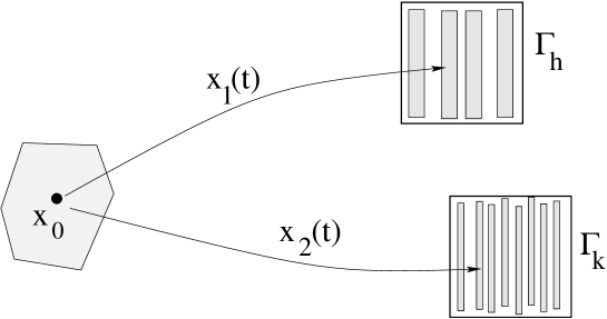
Figure 1: The terminal cost $\psi$ has uniformly bounded gradient. However, we can construct a perturbation $\psi^{\sharp}$ whose third derivatives have vastly different sizes on different cubes $\Gamma_{k}$ of the partition.

4. To help the reader, we first explain the heart of the matter, with the aid of Fig. 1. Let $\eta\in B_{K}$ be given. Assume that $x_{0}$ is an initial point from which two optimal trajectories $x_{1}(\cdot)$, $x_{2}(\cdot)$ originate. To fix ideas, assume

$$y_{1}\,=\,x_{1}(T)\in\Gamma^{\prime}_{h}\,,\qquad\qquad y_{2}\,=\,x_{2}(T)\,\in\,\Gamma^{\prime}_{k}\,,$$

with $h<k$. On $\Gamma_{k}^{\prime}$ the terminal cost function $\psi^{\sharp}$ has a much larger third derivative than on $\Gamma_{h}^{\prime}$. We observe that the Jacobian matrix of the map $y\mapsto x^{\eta}(0,y)$ is uniformly invertible in a neighborhood of $y_{1}$ and $y_{2}$. By the implicit function theorem, for all $x\in B(x_{0},\delta_{2})$, on a ball centered at $x_{0}$ with sufficiently small radius $\delta_{2}>0$, we can thus define the cost functions $\Phi_{1}(x)$, $\Phi_{2}(x)$, corresponding to trajectories $x_{1}(\cdot),x_{2}(\cdot)$ that start at $x$, satisfy the PMP, and terminate in a neighborhood of $y_{1}$, $y_{2}$, respectively. Since the terminal costs $\psi^{\sharp}\bigl{(}x_{i}(T)\bigr{)}$ of these trajectories have very different third order derivatives, we will show that the cost functions $\Phi_{1},\Phi_{2}$ also have different third order derivatives in a neighborhood of $x_{0}$. Therefore, the set of points where $\Phi_{1}(x)=\Phi_{2}(x)$ must be very small, regardless of the particular function $\eta(\cdot)$. A proof of these claims will be worked out with the aid of

Lemma 4.2

Consider a system of $n+n$ ODEs on the interval $[0,T]$,

$$\left\{\begin{array}[]{rl}\dot{x}(t)&=~{}F\bigl{(}t,x(t),p(t)\bigr{)},\\[5.69054pt] \dot{p}(t)&=~{}G\bigl{(}t,x(t),p(t)\bigr{)}.\end{array}\right.$$ (4.25)

Assume that all coefficients are uniformly bounded in ${\cal C}^{2}$.

• Consider a family of solutions $(x,p)(t,y)$ with initial data

  $$x(0)=y,\qquad p(0)=\varphi(y).$$ (4.26)

  Assume that $\varphi\in{\cal C}^{2}$ and the map $y\mapsto x(T,y)$ is uniformly invertible. More precisely, the norm of its $n\times n$ Jacobian matrix satisfies

  $$\Big{|}D_{y}x(T,y)\Big{|}\,\leq\,C,\qquad\qquad\Big{|}\bigl{[}D_{y}x(T,y)\bigr{]}^{-1}\Big{|}\,\leq\,C.$$ (4.27)

  Then the second derivatives $D^{2}_{x}p$ of the map $x(T,y)\mapsto p(T,y)$ satisfy a uniform bound, depending on the ${\cal C}^{2}$ norms of the functions $F,G,\varphi$, and on the constant $C$ in (4.27).

• Similarly, consider a family of solutions $(x,p)(t,y)$ with terminal data

  $$x(T)=y,\qquad p(T)=\varphi(y).$$ (4.28)

  Assume that $\varphi\in{\cal C}^{2}$ and the map $y\mapsto x(0,y)$ is uniformly invertible. More precisely, the norm of its $n\times n$ Jacobian matrix satisfies

  $$\Big{|}D_{y}x(0,y)\Big{|}\,\leq\,C,\qquad\qquad\Big{|}\bigl{[}D_{y}x(0,y)\bigr{]}^{-1}\Big{|}\,\leq\,C.$$ (4.29)

  Then the second derivatives $D^{2}_{x}p$ of the map $x(0,y)\mapsto p(0,y)$ satisfy a uniform bound, depending on the ${\cal C}^{2}$ norms of the functions $F,G,\varphi$, and on the constant $C$ in (4.29).

Proof. Part (ii) is entirely similar to part (i), after reversing the direction of time. We thus focus on a proof of (i).

Standard results on the higher order differentiability of solutions to ODEs, see for example Theorem 4.1 in [15], p.100, imply that the maps

$$y\mapsto x(T,y),\qquad\qquad y\mapsto p(T,y)$$ (4.30)

are twice continuously differentiable, and satisfy bounds of the form

$$\bigl{|}D^{2}_{y}x(T,y)\bigr{|}~{}\leq~{}C_{1},\qquad\qquad\bigl{|}D^{2}_{y}p(T,y)\bigr{|}~{}\leq~{}C_{1},$$

for some constant $C_{1}$ depending only on the ${\cal C}^{2}$ norms of $F,G,\varphi$. By assumption, the first map in (4.30) is invertible because of (4.27). As a consequence, the inverse function $x\mapsto y(x)$ is well defined, and has a bounded second derivatives, depending on the constants $C,C_{1}$.

This implies that the composed map $x\mapsto p\bigl{(}T,y(x)\bigr{)}$ is ${\cal C}^{2}$, and its second derivatives can be bounded in terms of the constants $C,C_{1}$. MM     

We now resume the proof of Theorem 4.1. 5. We finalize the construction of the perturbed terminal cost $\psi^{\sharp}$ by assigning the increasing sequence of numbers $M_{k}$.

We start by choosing $M_{1}>\|\psi\|_{{\cal C}^{3}}$. By induction, assume now that $M_{1},\ldots,M_{k-1}$ have been chosen.

Consider any trajectory satisfying the PMP, starting at some point $x\in B_{R}$ and ending inside some $\Gamma_{j}$ with $j\leq k-1$. We shall apply Lemma 4.2 in the special case where (4.25) is given by (4.6).

Calling $t\mapsto(x_{j},p_{j})(t,y)$ the solution to (4.6) with terminal condition $(x(T),p(T))=(y,\psi^{\sharp}(y))$ for $y\in\Gamma_{j}$. For $x=x_{j}(0,y)$, we define

$$\Phi_{j}(x)~{}\doteq~{}\int_{0}^{T}L\Big{(}x_{j}(t,y),u^{\eta}(t,x_{j}(t,y),p_{j}(t,y)),\eta(t)\Big{)}dt+\psi^{\sharp}(y).$$

Recalling (4.6) and (4.8), the derivative of the cost w.r.t. the terminal point of the trajectory is computed by

$$\begin{split}D\Phi_{j}(x)D_{y}x_{j}(0,y)&=~{}\int_{0}^{T}L_{x}\big{(}x_{j},u^{\eta},\eta\big{)}D_{z}x_{j}+L_{u}\big{(}x_{j},u^{\eta},\eta\big{)}{d\over dy}u^{\eta}dt+D\psi^{\sharp}(y)\\ &=~{}\int_{0}^{T}-{d\over dt}\left[p_{j}(t,y)D_{z}x_{j}(t,y)\right]dt+D\psi^{\sharp}(y)~{}=~{}p_{j}(0,y)D_{z}x_{y}(0,y).\end{split}$$

This implies

$$D\Phi_{j}(x)~{}=~{}D\Phi_{j}(x_{j}(0,y))~{}=~{}p_{j}(0,y)\,.$$

By part (ii) of Lemma 4.2, the a priori bound on (4.22) on the third derivative of $\psi^{\sharp}$ yields an a priori bound on the third derivative of the value function $D^{3}\Phi_{j}(x)$, for any $x=x_{j}(0,y)$ with $y\in\Gamma_{j}$. Say,

$$\bigl{|}D^{3}\Phi_{j}(x)\bigr{|}~{}\leq~{}M_{j}^{\prime}\,.$$ (4.31)

We now apply part (i) Lemma 4.2. This implies that, for any initial data (4.26), with $\|D^{2}\varphi\|_{{\cal C}^{2}}\leq M^{\prime}_{j}$, the solution to (4.25) satisfies a bound of the form

$$\bigl{|}D^{2}_{x}p(T,x)\bigr{|}~{}\leq~{}M_{j}^{\prime\prime}.$$ (4.32)

The constant $M_{k}$ is now chosen so that

$$M_{k}~{}>~{}\max\{M_{1}^{\prime\prime},\ldots,M_{k-1}^{\prime\prime}\}.$$ (4.33)

We observe the above construction achieves the following:

Consider two families of trajectories satisfying the PMP, starting in a neighborhood of the same point $x_{0}$, and ending in different cubes, say $\Gamma^{\prime}_{j}$ and $\Gamma^{\prime}_{k}$, with $j<k$. By the choice of $M_{k}$ at (4.33) and the bounds (4.31), at all initial points $y$ such that $x_{k}(T,y)\in\Gamma_{k}^{\prime}$, we have

$$\bigl{|}D^{3}\Phi_{j}(x)\bigr{|}~{}\leq~{}M_{j}^{\prime},\qquad\qquad\bigl{|}D^{3}\Phi_{k}(x)\bigr{|}~{}>~{}M_{j}^{\prime}\,.$$

Indeed, if the second inequality did not hold, then we would have the bound (4.32), contrary to the construction of $\psi^{\sharp}$.

Thus, the third derivatives $D^{3}\Phi_{j}(x)$ and $D^{3}\Phi_{k}(x)$ are strictly different in a neighborhood of $x_{0}$. 6. Based on the previous analysis, we give a bound on the Lebesgue measure of the set of initial points $x_{0}$ from which two distinct optimal trajectories initiate, ending in different cubes $\Gamma_{j},\Gamma_{k}$. This set contains:

• Points $x_{0}=x^{\eta}(0,y)$ with $y\in B(0,R_{0})$ such that the determinant of the Jacobian matrix $D_{y}x^{\eta}(0,y)$ is small:

  $$\bigl{|}\det\big{(}D_{y}x^{\eta}(0,y)\big{)}\bigr{|}~{}\leq~{}\delta_{1}\,.$$

  The Lebesgue measure of this set is $<\delta_{1}\cdot\hbox{meas}\bigl{(}B(0,R_{0})\bigr{)}$. Choosing $\delta_{1}$ small enough, since the probability measure $\mu_{0}$ is absolutely continuous, we achieve (4.24).

• Points $x_{0}\in B(0,R_{0})$ such that $x_{0}=x^{\eta}(0,y)$ for some $y\in\Gamma_{k}\setminus\Gamma^{\prime}_{k}$. By (4.20) it follows

  $$\hbox{meas}\left(\bigcup_{k=1}^{\nu}(\Gamma_{k}\setminus\Gamma^{\prime}_{k})\right)~{}<~{}\varepsilon_{1}\,.$$

  Again, since $\mu_{0}$ is absolutely continuous, by choosing $\varepsilon_{1}>0$ sufficiently small, we achieve

  $$\mu_{0}\left(\Big{\{}x^{\eta}(0,y)\,;~{}~{}y\in\bigcup_{k}(\Gamma_{k}\setminus\Gamma^{\prime}_{k})\Big{\}}\right)~{}<~{}{\varepsilon_{0}\over 2}\,.$$ (4.34)

  Toward (4.34), it is important to observe that the determinant of the Jacobian matrix $D_{y}x^{\eta}(0,y)$ satisfies a uniform bound, depending on the second derivatives $D^{2}\psi^{\sharp}$. By (4.19) these remain bounded, even when the third derivatives are changed.

• The remaining set $S$ of all points $x_{0}\in B(0,R_{0})$ which lie outside the previous two sets. We claim that $S$ has measure zero. Indeed, if $x_{0}\in S$ is the initial point for two trajectories satisfying the PMP and terminating inside two distinct sets $\Gamma_{j}^{\prime},\Gamma_{k}^{\prime}$, then the corresponding value functions $\Phi_{j},\Phi_{k}$ has distinct third derivative at $x_{0}$. Therefore, $x_{0}$ cannot be a Lebesgue point of the coincidence set $\{x\,;~{}\Phi_{j}(x)=\Phi_{k}(x)\}$. Since the set has no Lebesgue points, it has measure zero. By the absolute continuity of $\mu_{0}$, we obtain

  $$\mu_{0}(S)=0.$$ (4.35)

Combining the three bounds (4.24), (4.34), and (4.35), this achieves the proof. MM     

5 Examples of structurally stable solutions

In this section we give some examples of first order mean field games with one or more solutions, and discuss their stability.

To motivate the examples concerning differential games, we first consider two maps of the unit disc $B_{1}\subset I\!\!R^{2}$ onto itself, in polar coordinates $(r,\theta)$.

$$\phi_{1}(r,\theta)~{}=~{}\left({2r\over 1+r^{2}}\,,~{}\theta+\theta_{0}\right),\qquad\qquad\phi_{2}(r,\theta)~{}=~{}\left({r\over 1+r^{2}}\,,~{}\theta\right),$$ (5.1)

where the rotation angle satisfies $0<\theta_{0}<2\pi$. Notice that the origin is the unique fixed point of both $\phi_{1}$ and $\phi_{2}$. However, this fixed point is asymptotically stable for the map $\phi_{2}$, but unstable for $\phi_{1}$. Indeed, for every $\bar{r}\geq 0$, the sequence of radii

$$r_{n+1}~{}=~{}{r_{n}\over 1+r_{n}^{2}},\qquad r_{0}~{}=~{}\bar{r},$$

is decreasing and converges to $0$. On the other hand, for $0<\bar{r}<1$, the sequence

$$r_{n+1}~{}=~{}{2r_{n}\over 1+r_{n}^{2}},\qquad r_{0}~{}=~{}\bar{r},$$

is increasing and converges to $1$.

5.1 Games with a unique solution, stable or unstable.

In the following examples of mean field games, as probability space labeling the various players we simply take $\Omega=[0,1]$. Motivated by (5.1), we begin by constructing mean field games with a unique solution, which is unstable in the first example, and stable in the second.

Example 5.1

Consider a game where each player $\xi\in[0,1]$ minimizes the same cost

$$J(u)~{}=~{}\int_{0}^{T}|u(t)|^{2}\,dt+\bigl{|}x(T)-\psi(b(T))\bigr{|}^{2},$$ (5.2)

subject to the trivial dynamics

$$\dot{x}(t)~{}=~{}u(t),$$ (5.3)

with initial data

$$x(\xi,0)~{}=~{}\bar{x}(\xi)~{}=~{}0\qquad\hbox{for all}~{}\xi\in[0,1].$$ (5.4)

Here $u(t),x(t)\in I\!\!R^{2}$ while, as in (3.3), $b(T)\in I\!\!R^{2}$ denotes the barycenter of the terminal positions of all players. Two cases will be considered.

1 - An unstable game. Let the terminal cost be

$$\psi(x)~{}=~{}{1+T\over T}\cdot\phi_{1}(x),$$

where $\phi_{1}$ is the first map defined at (5.1), using polar coordinates. In this case, $x(t,\xi)\equiv 0$ for all $(t,\xi)\in[0,T]\times[0,1]$ provides the unique solution to the mean field game. Indeed, given a barycenter $b(T)$, the PMP

$$\left\{\begin{array}[]{rl}\dot{x}&=-\displaystyle{p\over 2}\,,\\[8.53581pt] \dot{p}&=~{}0,\end{array}\right.\qquad\mathrm{with}\qquad\begin{cases}x(0)&=0\,,\\[8.53581pt] p(T)&=2(x(T)-\psi(b(T))),\end{cases}$$ (5.5)

has a unique solution

$$x(t)~{}=~{}{t\over 1+T}\cdot\psi(b(T))\qquad t\in[0,T].$$ (5.6)

All the optimal trajectories $x(\cdot,\xi)$ of the mean field game are the same. In particular, if $x^{*}(t,\xi)$ is a solution to the game then

$$b^{*}(T)~{}=~{}\int_{0}^{1}x^{*}(T,\xi)d\xi~{}=~{}x^{*}(T,\xi)~{}=~{}{T\over 1+T}\cdot\psi(b^{*}(T))~{}=~{}\phi_{1}(b^{*}(T)).$$

Notice that $\phi_{1}$ has a unique fixed point, i.e. the origin, we have $b^{*}(T)=0$ and (5.6) yields $x^{*}(\cdot,\xi)\equiv 0$ for all $\xi\in[0,1]$. On the other hand, for any sequence $b^{(k)}$ such that $b^{(k+1)}=\Phi(b^{(k)})$, one has that

$$b^{(k+1)}(T)~{}=~{}{\kappa T\over 1+\kappa T}\cdot\psi\big{(}b^{(k)}(T)\big{)}~{}=~{}\phi\big{(}b^{(k)}(T)\big{)}.$$

Since $0$ is an unstable equilibrium of $\phi$, the zero solution of game is unstable.

2 - A stable game. Similarly, if the terminal cost $\psi$ is given by

$$\psi(x)~{}=~{}{1+T\over T}\cdot\phi_{2}(x)$$

with $\phi_{2}$ being the first map in (5.1) then $x^{*}(\xi,\cdot)\equiv 0$ for all $\xi\in[0,1]$ is again the unique solution of the MFG. Moreover, since $0$ is asymptotically stable for the map $\phi_{2}$, the solution $x^{*}$ is stable.

5.2 Games with multiple solutions.

Next, we give an example of a mean field game which admits both stable and unstable (but structurally stable) solutions.

Example 5.2

Here all controls and trajectories are scalar functions. The objective of every player is

$$\hbox{minimize:}\quad\int_{0}^{T}\left[|u(t)|^{2}+{1\over 1+x^{2}(t)}+\kappa\cdot\bigl{|}x(t)-b(t)\bigr{|}^{2}\right]\,dt,$$ (5.7)

subject to

$$\dot{x}~{}=~{}u,\qquad\qquad x(0,\xi)~{}=~{}0\qquad\hbox{for all}~{}\xi\in[0,1].$$ (5.8)

Here $b$ denotes the barycenter of the distribution of players as in (3.3).

Proposition 5.1

For the MFG (5.7)–(5.8), the following holds.

• For all $\kappa>1$ and $T>2$, the mean field game has at least three solutions. These have the form

  $$x_{i}(t,\xi)~{}=~{}y_{i}(t),\qquad\qquad i=0,1,2,$$ (5.9)

  with $y_{0}(t)=0$, while $y_{1}$ is monotone increasing, and $y_{2}(t)=-y_{1}(t)$ for $t\in[0,T]$.

• The zero solution is unstable. However, assuming that $T\not={(2n-1)\pi\over 2}$ for every $n\geq 1$, this solution is structurally stable.

• Both solutions $x_{1},x_{2}$ are stable, and structurally stable.

Proof. 1. Given a function $b(\cdot)$, the reduced Hamiltonian of (5.7)-(5.8) is computed by

$$\widehat{H}^{b}(x,p,t)~{}=~{}{1\over 1+x^{2}}+\kappa\cdot\bigl{|}x-b(t)\bigr{|}^{2}-{p^{2}\over 2}.$$

Assume that $\kappa>1$. For every $p\in I\!\!R,t\geq 0$, we have

$$\widehat{H}_{xx}^{b}(x,p,t)~{}=~{}2\cdot\left(\kappa-{1\over(1+x^{2})^{2}}+{4x^{2}\over(1+x^{2})^{3}}\right)~{}>~{}0\qquad\hbox{for all}~{}x\in I\!\!R,$$

hence the map $x\mapsto\widehat{H}^{b}(x,p,t)$ is strictly convex. Thus, by the same argument in Step 2 of the proof of Theorem 3.1, the optimal control problem (5.7)–(5.4) has a unique optimal solution and all the optimal trajectories $x(\cdot,\xi)$ of the mean field game coincide. As a consequence, $x(\cdot,\xi)=b(\cdot)$ is an optimal solution to the optimization problem

$$\hbox{minimize:}\quad\int_{0}^{T}\left[{|\dot{x}|^{2}\over 2}+{1\over 2\bigl{(}1+x^{2}(t)\bigr{)}}\right]\,dt,\quad\hbox{subject to}\quad x(0)~{}=~{}0.$$ (5.10)

Here, we can think of

$$K(\dot{x})~{}=~{}{\dot{x}^{2}\over 2}\,,\qquad\qquad V(x)~{}=~{}-{1\over 2(1+x^{2})}$$

respectively as kinetic and potential energy. The solution is a motion governed by the Euler-Lagrange equations

$$\ddot{y}(t)\,=\,-V_{y}(y)\,=\,-{y(t)\over\big{[}1+y^{2}(t)\big{]}^{2}},\qquad\qquad y(0)\,=\,0,\qquad\dot{y}(T)\,=\,0.$$ (5.11)

It is clear that $y\equiv 0$ is a solution of (5.11) and this provides the first solution of the mean field game

$$x(t,\xi)~{}=~{}0\qquad\hbox{for all}~{}\xi\in[0,1],\quad t\in[0,T].$$ (5.12)

To complete this step, we claim that (5.11) admits at least two additional solutions $y_{1}(\cdot)$, $y_{2}(\cdot)$, such that $y_{1}$ is strictly increasing in $[0,T]$, and $y_{2}(t)=-y_{1}(t)$ . The mean field game has two more solutions $x_{1},x_{2}$, as in (5.9).

Observe that solutions to the Euler-Lagrange equations conserve the total energy

$$E(y,\dot{y})~{}=~{}K(\dot{y})+V(y)~{}=~{}{\dot{y}^{2}\over 2}-{1\over 2(1+y^{2})}\,.$$ (5.13)

Level sets where $E$ is constant are plotted in Fig. 2. Solutions to the boundary value problem (5.11) correspond to trajectories that start at time $t=0$ on the vertical axis where $y=0$, and end at time $t=T$ on the horizontal axis where $\dot{y}=0$.

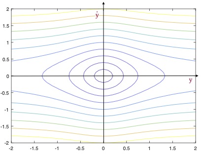
Figure 2: The level sets where the energy $E(y,\dot{y})$ at (5.13) is constant.

We thus seek an increasing solution of

$$\dot{y}(t)~{}=~{}\sqrt{{1\over 1+y^{2}(t)}-{1\over 1+M^{2}}},\qquad\qquad y(0)~{}=~{}0,$$ (5.14)

for some constant $M$ such that $M=y(T)$. Calling $y=y(t,c)$ the solution to (5.14) with $M=c$, we have

$${\sqrt{c}\over 1+c^{2}}\cdot\sqrt{c-y(t,c))}~{}\leq~{}\dot{y}(t,c)~{}\leq~{}\sqrt{{2c\over 1+c^{2}}}\cdot\sqrt{c-y(t,c))}.$$

By a comparison argument, we obtain for all $0\leq t\leq\sqrt{2(1+c^{2})}$ that

$$c-c\cdot\left(1-{t\over 2(1+c^{2})}\right)^{2}~{}\leq~{}y(t,c)~{}\leq~{}c-c\cdot\left(1-{t\over\sqrt{2(1+c^{2})}}\right)^{2}.$$ (5.15)

In particular, assume that $T>\sqrt{2}$. For every $c\geq\sqrt{{T^{2}-2\over 2}}$, the solution $y(\cdot,c)$ is defined on $[0,T]$ and satisfies

$$c\cdot\left(1-\left(1-{1\over T}\right)^{2}\right)~{}\leq~{}y(T,c)~{}\leq~{}c.$$

Calling $M\doteq\inf\left\{c\geq\sqrt{{T^{2}-2\over 2}}:y(T,c)\leq c\right\}>0$, we claim that $y(T,M)=M$. Indeed, assume that $M-y(T,M)=\delta_{0}>0$. Then, by (5.15), one has

$$M-\delta_{0}~{}=~{}y(T,M)~{}\leq~{}M\cdot\left(1-\left(1-{T\over\sqrt{2(1+M^{2})}}\right)^{2}\right).$$

Hence, $M-\displaystyle\sqrt{T^{2}-2\over 2}=\varepsilon_{0}>0$ and the map $t\mapsto y(t,M-\varepsilon)$ is defined on $[0,T]$ for all $0<\varepsilon<\varepsilon_{0}$. Moreover, by the monotone increasing property of $c\mapsto y(T,c)$, we have

$$y(T,M-\varepsilon)~{}\leq~{}y(T,M)~{}=~{}M-\delta_{0}~{}\leq~{}M-\varepsilon$$

for all $0<\varepsilon<\min\{\varepsilon_{0},\delta_{0}\}$. This yields a contradiction.

In the next steps we will show that all three solutions are essential, the zero solution is unstable, and the two non-zero solutions are stable.

2. We begin by showing that the null solution $x(t,\xi)\equiv 0$ is unstable but essential. In the present case, the map $b\mapsto\widetilde{b}=\Phi(b)$ at (1.7)-(1.8) takes the form

$$\Phi(b)(t)~{}=~{}x_{b}(t)\qquad\hbox{for all}~{}t\in[0,T],$$

where $(x_{b},p_{b})$ denotes the unique solution of the PMP

$$\left\{\begin{array}[]{rl}\dot{x}&=~{}u(x,p)~{}=~{}-\displaystyle{p\over 2},\\[8.53581pt] \dot{p}&=~{}\displaystyle{2x\over(1+x^{2})^{2}}-2\kappa\cdot(x-b),\end{array}\right.\qquad\left\{\begin{array}[]{rl}x(0)&=~{}0,\\[8.53581pt] p(T)&=~{}0,\end{array}\right.$$ (5.16)

where the optimal control is

$$u(x,p)~{}=~{}\hbox{arg}\!\min_{\omega\in I\!\!R}\Big{\{}\omega^{2}+p\,\omega\Big{\}}~{}=~{}-{p\over 2}.$$

Linearizing the system (5.16) at $b\equiv 0$ we obtain an expression for the differential $D\Phi(0)$, namely

$$D\Phi(0)\,b~{}=~{}\widehat{b},$$

where $\widehat{b}(t)=X(t)$ is the function obtained by solving the linear system

$$\begin{bmatrix}\dot{X}(t)\\[11.38109pt] \dot{P}(t)\end{bmatrix}~{}=~{}\begin{bmatrix}0&-1/2\\[11.38109pt] 2-2\kappa&0\end{bmatrix}\begin{bmatrix}X(t)\\[11.38109pt] P(t)\end{bmatrix}+2\kappa b(t)\begin{bmatrix}0\\[11.38109pt] 1\end{bmatrix},\qquad X(0)~{}=~{}P(T)~{}=~{}0.$$ (5.17)

Eliminating the variable $P=-2\dot{X}$, one is led to the second order ODE

$$-2\ddot{Y}~{}=~{}(2-2\kappa)Y+2\kappa b.$$

To determine eigenvalues $\lambda$ and eigenfunctions $Y$, we need to solve

$$-2\ddot{Y}=(2-2\kappa)Y+{2\kappa\over\lambda}\,Y,\qquad\qquad Y(0)\,=\,\dot{Y}(T)\,=\,0.$$

$$\ddot{Y}+\left(1-\kappa+{\kappa\over\lambda}\right)Y~{}=~{}0,\qquad\qquad Y(0)\,=\,\dot{Y}(T)\,=\,0.$$ (5.18)

The eigenvalues and eigenfunctions of $D\Phi(0)$ are thus found to be

$$\lambda_{n}~{}=~{}{\kappa\over\kappa+{(2n-1)^{2}\pi^{2}\over 4T^{2}}-1}\,,\qquad\qquad Y_{n}(t)~{}=~{}\sin\left({(2n-1)\pi\over 2T}t\right),\qquad n=1,2,\dots.$$ (5.19)

In particular, if $T>\displaystyle{\pi\over 2}$ and $\kappa>1$, computing the first eigenvalue of $D\Phi(0)$ one finds $\lambda_{1}>1$. This implies that the null solution $x(t,\xi)\equiv 0$ is unstable.

On the other hand, we observe that, by (5.19), if

$$T\,\not=\,{(2n-1)\pi\over 2}\qquad\qquad\hbox{for every}~{}n\geq 1,$$ (5.20)

then $1$ is not an eigenvalue of $D\Phi(0)$. In this case, using the same argument as in Step 4 of the proof of Theorem 3.1, we conclude that $y_{1}$ is essential.

3. We now prove that $y_{1}$ is stable. Given any ${\bf b}\in\mathcal{C}([0,T])$, we first compute $D\Phi(y_{1})(\bar{b})$. As in step 2, for every $\varepsilon\in I\!\!R$, let $(x^{\varepsilon}(t),p^{\varepsilon}(t))$ be the solution of $(\ref{PMP-EX1})$ with $b=y_{1}+\varepsilon\bar{b}$. By the linearization, it holds

$$\begin{bmatrix}x^{\varepsilon}(t)\\[11.38109pt] p^{\varepsilon}(t)\end{bmatrix}~{}=~{}\begin{bmatrix}y_{1}(t)\\[11.38109pt] p_{1}(t)\end{bmatrix}+\varepsilon\,\begin{bmatrix}{\bf x}_{\bar{b}}(t)\\[11.38109pt] {\bf p}_{\bar{b}}(t)\end{bmatrix}+o(\varepsilon).$$

Here $\begin{bmatrix}{\bf x}_{\bar{b}}(t)\\ {\bf p}_{\bar{b}}(t)\end{bmatrix}$ is the solution to the equation obtained linearizing (5.16) around $y_{1}$, namely

$$\begin{cases}\dot{\bf x}(t)~{}=~{}-\displaystyle{{\bf p}(t)\over 2}\,,\\[8.53581pt] \dot{\bf p}(t)~{}=~{}\displaystyle 2\left({1-3y_{1}^{2}\over(1+y_{1}^{2})^{3}}-\kappa\right){\bf x}+2{\kappa}\bar{b}\,,\end{cases}\qquad\begin{cases}{\bf x}(0)~{}=~{}0,\\[8.53581pt] {\bf p}(T)~{}=~{}0.\end{cases}$$ (5.21)

Let the pair $(\gamma,\bar{b})$ denote an eigenvalue and an eigenfunction of $D\Phi(y_{1})$. As in Step 2, we have

$$D\Phi(y_{1})(\bar{b})~{}=~{}{\bf x}_{\bar{b}}~{}=~{}\gamma\bar{b},$$

and ${\bf x}_{\bar{b}}$ solves the two point boundary problem

$$\ddot{y}(t)~{}=~{}\left[\kappa\cdot\left(1-{1\over\gamma}\right)+{3y_{1}^{2}-1\over(1+y^{2}_{1})^{3}}\right]\cdot y(t),\qquad y(0)~{}=~{}\dot{y}(T)~{}=~{}0.$$ (5.22)

To verify the stability of $y_{1}$, we will show that all eigenvalues of $D\Phi(y_{1})$ are contained within the open interval $]0,1[$. Assume by a contradiction that $D\Phi(y_{1})$ has an eigenvalue $\gamma\in I\!\!R\setminus\,]0,1[\,$, so that the equation (5.22) has a nonzero solution $y_{2}$. Recalling that $t\mapsto y_{1}(t)\in[0,+\infty[$ is strictly increasing with $y_{1}(0)=0$, we define

$$t_{1}~{}\doteq~{}\min\left\{t\in[0,T]:\kappa\cdot\left(1-{1\over\gamma}\right)+{3y_{1}^{2}(t)-1\over(1+y^{2}_{1})^{3}(t)}\geq 0\right\}.$$

For every $\tau\in[t_{1},T]$, from (5.22) it follows

$$-y_{2}(\tau)\dot{y}_{2}(\tau)~{}=~{}\int_{\tau}^{T}\dot{y}_{2}^{2}(t)dt+\int_{\tau}^{T}\kappa\cdot\left(1-{1\over\gamma}\right)+{3y_{1}^{2}-1\over(1+y^{2}_{1})^{3}}y_{2}^{2}(t)dt~{}>~{}0.$$

Therefore, both $y$ and $\dot{y}$ do not change sign in $[t_{1},T]$. Without loss of generality, we can assume that $y$ is positive in $[t_{1},T]$. Set

$$t_{2}~{}\doteq~{}\max\bigl{\{}t\in[0,t_{1}]:y_{2}(t)~{}=~{}0\bigr{\}}.$$

We then have

$$y_{2}^{\prime}(t_{2})~{}>~{}0,\qquad y_{2}(t_{2})~{}=~{}0,\qquad\mathrm{and}\qquad y_{2}(t)~{}\geq~{}0\qquad\hbox{for all}~{}t\in[t_{2},T].$$

On the other hand, since $y_{1}$ is an increasing solution of (5.11), the function $z_{1}\doteq\dot{y}_{1}$ solves the equation

$$\ddot{z}(t)~{}=~{}{3y_{1}^{2}-1\over(1+y^{2}_{1})^{3}}\cdot z(t),~{}~{}~{}\qquad\dot{z}(0)~{}=~{}z(T)~{}=~{}0.$$

Thus, for all $t\in[t_{2},T]$, one has

$$[\dot{y}_{2}(t)z_{1}(t)]^{\prime}~{}=~{}[\dot{z}_{1}(t)y_{2}(t)]^{\prime}+\left(1-{1\over\gamma}\right)y_{2}(t)z_{2}(t)~{}\geq~{}[\dot{z}_{1}(t)y_{2}(t)]^{\prime},$$

and this yields

$$\dot{y}_{2}(t)z_{1}(t)-\dot{y}_{2}(t_{2})z_{1}(t_{2})~{}\geq~{}\dot{z}_{1}(t)y_{2}(t).$$ (5.23)

Equivalently,

$${d\over dt}\left({y_{2}(t)\over z_{1}(t)}\right)~{}\geq~{}\dot{y}_{2}(t_{2})z_{1}(t_{2})\cdot{1\over z_{1}^{2}(t)}\qquad\hbox{for all}~{}t\in[t_{2},T].$$

This implies

$$y_{2}(t)~{}\geq~{}\dot{y}_{2}(t_{2})z_{1}(t_{2})\cdot\int_{t_{2}}^{t}{1\over z_{1}^{2}(t)}dt.$$

Therefore, by (5.23) one has

$$\dot{y}_{2}(t)~{}\geq~{}\dot{y}_{2}(t_{2})z_{1}(t_{2})\cdot\left[{1\over z_{1}(t)}+\dot{z}_{1}(t)\cdot\int_{0}^{t}{1\over z^{2}_{1}(s)}ds\right].$$ (5.24)

To obtain a contradiction, we will show that

$$0~{}=~{}\dot{y}_{2}(T)~{}=~{}\dot{y}_{2}(t_{2})z_{1}(t_{2})\cdot\lim_{t\to T-}\left[{1\over z_{1}(t)}+\dot{z}_{1}(t)\cdot\int_{0}^{t}{1\over z^{2}_{1}(s)}ds\right]~{}>~{}0.$$ (5.25)

Assume that $y_{1}(0)=v_{0}$ and $\beta=y_{1}(T)$. We then have

$$z_{1}(t)~{}=~{}\dot{y}_{1}(t)~{}=~{}\left(v_{0}^{2}-{y^{2}_{1}(t)\over 1+y^{2}_{1}(t)}\right)^{1/2},\qquad v_{0}^{2}~{}=~{}{\beta^{2}\over 1+\beta^{2}}\,,$$

and

$$\dot{z}_{1}(t)~{}=~{}\ddot{y}_{1}(t)~{}=~{}-{y_{1}(t)\over(1+y^{2}_{1}(t))^{2}}.$$

By a change of variable, (5.25) is equivalent to

$$I~{}\doteq~{}\lim_{y\to\beta-}\left[{(1+\beta^{2})^{1/2}(1+y^{2})^{1/2}\over(\beta+y)^{1/2}(\beta-y)^{1/2}}-{y\over(1+y^{2})^{2}}\cdot\int_{0}^{y}{(1+\beta^{2})^{3/2}(1+z^{2})^{3/2}\over(\beta+z)^{3/2}(\beta-z)^{3/2}}dz\right]~{}>~{}0.$$

Notice that for $\beta>0$ sufficiently large, we have

$$\lim_{y\to\beta}\left[{(1+\beta^{2})^{1/2}(1+y^{2})^{1/2}\over(\beta+y)^{1/2}(\beta-y)^{1/2}}-{1+\beta^{2}\over\sqrt{2\beta}(\beta-y)^{1/2}}\right]~{}=~{}0\,,$$

and

$${y\over(1+y^{2})^{2}}\cdot\int_{0}^{y}{(1+\beta^{2})^{3/2}(1+z^{2})^{3/2}\over(\beta+z)^{3/2}(\beta-z)^{3/2}}dz \leq {y(1+\beta^{2})^{3/2}\over(1+y^{2})^{1/2}(\beta+y)^{3/2}}\int_{0}^{y}(\beta-z)^{3/2}dz$$

$$= {2y(1+\beta^{2})^{3/2}\over(1+y^{2})^{1/2}(\beta+y)^{3/2}}\cdot\left[{1\over(\beta-y)^{1/2}}-{1\over\beta^{1/2}}\right].$$

In particular, this implies

$$I~{}\geq~{}{1+\beta^{2}\over\beta\sqrt{2}}+(1+\beta^{2})\cdot\lim_{y\to\beta-}\left({1\over\sqrt{2\beta}}-{2y(1+\beta^{2})^{1/2}\over(1+y^{2})^{1/2}(\beta+y)^{3/2}}\right)\cdot{1\over\beta-y}~{}=~{}{1+\beta^{2}\over\beta\sqrt{2}}~{}>0~{}.$$

This shows that all eigenvalues of $D\Phi(y_{1})$ are contained in the open interval $]0,1[\,$, and $y_{1}$ is a stable solution of the MFG. By symmetry, $x_{2}(t,\xi)~{}=~{}y_{2}(t)\doteq-y_{1}(t)$ for $t\in[0,T]$ and all $\xi\in[0,1]$, is also a stable solution of the MFG. MM     

5.3 Examples of games with no solutions.

Example 5.3

Consider the mean field game on the time interval $t\in[0,T]$, where player $\xi\in\Omega=[0,1]$ has dynamics

$$\dot{x}~{}=~{}u~{}\in~{}[-1,1],\qquad x(0,\xi)~{}=~{}0.$$ (5.26)

The goal of player $\xi$ is to optimize his terminal position relative to the distribution of the other players, namely

$$\hbox{maximize:}\qquad\bigl{|}x(T,\xi)-b(\xi)\bigr{|}^{2},$$ (5.27)

where

$$b(\xi)~{}=~{}\int_{0}^{1}e^{-|\zeta-\xi|^{2}}\cdot x(T,\zeta)\,d\zeta.$$ (5.28)

We claim that this game has no strong solution. Indeed, if $b(\xi)\equiv 0$, then every player has two equally good strategies:

$$u(t)\equiv 1,\qquad x_{2}(t)=t\qquad\hbox{or}\qquad u(t)\equiv-1,\qquad x_{2}(t)=-t.$$ (5.29)

This cannot be a solution, because $\xi\mapsto x(T,\xi)\in\{-T,T\}$ is a measurable map, and the integral in (5.28) cannot be identically zero.

On the other hand, if $b(\xi)$ is not identically zero, then

$$\int_{0}^{1}b(\xi)\,x(T,\xi)\,d\xi~{}=~{}\int_{0}^{1}b(\xi)\cdot(-T\hbox{sign}\,b(\xi)\bigr{)}\,d\xi~{}=~{}-T\int_{0}^{1}\bigl{|}b(\xi)\bigr{|}\,d\xi~{}<~{}0.$$

However, the definition of $b$ implies

$$\begin{array}[]{rl}\displaystyle\int_{0}^{1}b(\xi)\,x(T,\xi)\,d\xi&\displaystyle=~{}\int_{0}^{1}\left(\int_{0}^{1}x_{2}(T,\zeta)e^{-|\zeta-\xi|^{2}}\,d\zeta\right)x(T,\xi)\,d\xi\\[11.38109pt] &\displaystyle=~{}\displaystyle\int_{0}^{1}\int_{0}^{1}e^{-|\zeta-\xi|^{2}}\,x(T,\zeta)\,x(T,\xi)\,d\zeta d\xi~{}\geq~{}0,\end{array}$$

reaching a contradiction. Notice that here the unique mild solution is a measure, where each player uses the two controls in (5.29) with equal probability.

Example 5.4

Consider the mean field game on the time interval $t\in[0,T]$, where all players have the same dynamics and the same cost functional:

$$\hbox{minimize:}\qquad\int_{0}^{T}u^{2}(t)\,dt+\psi\bigl{(}x(T)\bigr{)},$$ (5.30)

subject to

$$\dot{x}~{}=~{}u-b^{2},\qquad\quad|u(t)|\leq 1,\qquad\qquad x(0,\xi)~{}=~{}0\qquad\hbox{for all}~{}\xi\in\Omega\,,$$ (5.31)

and with terminal constraint

$$\varphi(x(T)\bigr{)}~{}\doteq~{}\bigl{(}T-x(T)\bigr{)}\cdot x(T)~{}=~{}0.$$ (5.32)

Here

$$b(t)~{}\doteq~{}\int_{\Omega}x(t,\xi)\,d\xi$$ (5.33)

denotes the barycenter of the distribution of players at time $t$, while the terminal cost is a smooth function that satisfies

$$\psi(x)~{}=~{}\left\{\begin{array}[]{cl}0&\hbox{if}\quad x=0,\cr-2T&\hbox{if}\quad x=T.\end{array}\right.$$ (5.34)

Notice that the terminal constraint (5.32) is equivalent to

$$x(T)~{}\in~{}\{0,T\}.$$ (5.35)

We claim that this mean field game has no solution. Namely, the “best reply map” ${\bf X}\mapsto\Psi({\bf X})$ from ${\bf L}^{1}\Big{(}\Omega\,;~{}{\cal C}\bigl{(}[0,T];\,I\!\!R^{n}\bigr{)}\Big{)}$ into itself does not have any fixed point. To prove this, consider first the case where ${\bf X}={\bf 0}\in{\bf L}^{1}\Big{(}\Omega\,;~{}{\cal C}\bigl{(}[0,T];\,I\!\!R^{n}\bigr{)}\Big{)}$. That means:

$$x(t,\xi)~{}=~{}0\qquad\hbox{for all ~{}~{} $t\in[0,T]$~{}~{}and ~{}~{}$\mu$-a.e.~{}$\xi\in\Omega$.}$$ (5.36)

In this case, $b(t)=0$ for all $t\in[0,T]$. Hence the optimal strategy for every player is to choose $u(t,\xi)=1$. The corresponding trajectory $x(t,\xi)=t$ satisfies the terminal constraint (5.32) and achieves minimum cost

$$J_{\min}~{}=~{}\int_{0}^{T}1\,dt+\psi(T)~{}=~{}T-2T~{}=~{}-T.$$

On the other hand, if (5.36) fails, then $b(t)$ is not identically zero and the solution to (5.31) cannot attain the value $x(T)=T$. Hence the best strategy for every player is to take $u(t,\xi)\equiv 0$, which yields the trajectory $x(t,\xi)=0$, with zero cost.

We have thus shown that

$${\bf 0}~{}\notin~{}\Psi({\bf 0}),\qquad\hbox{while}\quad\Psi({\bf X})~{}=~{}\{{\bf 0}\}\quad\hbox{for all}~{}~{}{\bf X}\not={\bf 0},$$

hence $\Psi$ cannot have a fixed point.

Notice that in this example the mean field game does not even admit mild solutions, in the randomized sense.

We observe that in this example, the minimum cost does not depend continuously on the parameter $b(\cdot)$. Namely, it jumps from $0$ down to $-T$ as $b$ becomes the zero function. This is due to a lack of transversality in connection with the terminal constraint.

6 Concluding remarks

In this paper we considered a class of first order mean field games, characterized by 5-tuples $(f,L,\psi,\phi,\bar{x})$ specifying the dynamics, cost functionals, averaging kernels, and initial distribution of players.

The main results show that, generically, for every given $\eta(\cdot)$ a.e. player has a unique optimal control $t\mapsto u^{\eta}(t,\xi)$. As a consequence, the “best reply” map $\eta\mapsto\Phi(\eta)$ at (1.8) is single valued, and the MFG has a strong solution. Moreover, there are open sets of games with unique solutions, and open sets of games with multiple solutions. These can be stable, or unstable, in the sense of Definition 1.2.

It would be of interest to analyze whether similar results remain valid in a more general setting. Namely:

• Systems with fully nonlinear dynamics, i.e. where the function $f(x,u,\eta)$ in (1.5) is not necessarily affine w..r.t. the control.

• Optimal control problems in the presence of terminal constraints, say

  $$g_{i}\bigl{(}x(T,\xi)\bigr{)}~{}=~{}0,\qquad\qquad i=1,\ldots,N.$$

In all our previous examples, the mean field games had structurally stable solutions. We thus conclude the paper with a natural conjecture:

Conjecture 6.1

For a generic 5-tuple $(f,L,\psi,\phi,\bar{x})\in{\cal X}$, the MFG (1.3)–(1.6) has finitely many solutions, all of which are structurally stable.

References

[1] M. Bardi and M. Fischer, On non-uniqueness
and uniqueness of solutions in finite-horizon mean field games. ESAIM Control Optim. Calc. Var.25 (2019), Paper No. 44.
[2]
M. Bardi and I. Capuzzo Dolcetta, Optimal Control and Viscosity
Solutions of Hamilton-Jacobi-Bellman Equations, Birkhäuser, Boston, 1997.
[3] J. M. Bloom, The local structure of smooth maps of manifolds.
B.A. thesis, Harvard 2004.
www.math.harvard.edu/theses/phd/bloom/ThesisXFinal.pdf
[4]
A. Bressan and B. Piccoli, Introduction to the Mathematical
Theory of Control,
AIMS Series in Applied Mathematics, Springfield Mo. 2007.
[5] A. Briani and P. Cardaliaguet,
Stable solutions in potential mean field game systems.
Nonlin. Diff. Equat. Appl.25 (2018), no. 1, Paper No. 1.
[6] P. Cannarsa and R. Capuani,
Existence and uniqueness for mean field games with state constraints.
In PDE models for multi-agent phenomena, pp. 49–71,
Springer INdAM Ser. 28, Springer, 2018.
[7] P. Cannarsa, R. Capuani, P. and Cardaliaguet,