Provable Sample-Efficient Sparse Phase Retrieval Initialized by Truncated Power Method
Abstract
We study the sparse phase retrieval problem, recovering an -sparse length- signal from magnitude-only measurements. Two-stage non-convex approaches have drawn much attention in recent studies. Despite non-convexity, many two-stage algorithms provably converge to the underlying solution linearly when appropriately initialized. However, in terms of sample complexity, the bottleneck of those algorithms with Gaussian random measurements often comes from the initialization stage. Although the refinement stage usually needs only measurements, the widely used spectral initialization in the initialization stage requires measurements to produce a desired initial guess, which causes the total sample complexity order-wisely more than necessary. To reduce the number of measurements, we propose a truncated power method to replace the spectral initialization for non-convex sparse phase retrieval algorithms. We prove that measurements, where is the stable sparsity of the underlying signal, are sufficient to produce a desired initial guess. When the underlying signal contains only very few significant components, the sample complexity of the proposed algorithm is and optimal. Numerical experiments illustrate that the proposed method is more sample-efficient than state-of-the-art algorithms.
-
April 2023
1 Introduction
In this paper, we consider the real-valued phase retrieval problem, which aims at recovering a high-dimensional signal from a system of phaseless measurements. That is, the task is to recover from the system
| (1) |
where are the sensing vectors and are the observations. The phase retrieval problem has arisen in various applications, for instances, X-ray crystallography [22], optics [48], microscopy [34], and others [19, 40]. In those applications, it is easier to record the intensity of the measurements due to hardware limitations, which leads to the phase retrieval problem (1).
When there is no prior assumption on , there may be infinitely many possible solutions to (1) if . To ensure the well-posedness of the problem, an oversampling (i.e., ) technique is applied. It has been shown that measurements are necessary and sufficient for a unique recovery (up to a global phase) with generic real sensing vectors [4]. Moreover, recent studies further indicate that the oversampling is required for both practical algorithms [15, 47, 20, 21, 2, 37, 16, 17, 55, 49, 13] and global landscape analysis [43, 28, 6, 7, 9, 8] to guarantee a successful recovery.
Meanwhile, the over-complete measurements naturally result in a huge sampling and computation cost in high-dimensional applications. Recently, it has been a great interest to further reduce the required number of measurements (or sample size) for phase retrieval problem [51, 38, 14, 39, 1, 24]. To recover the underlying signal with underdetermined measurements , a common approach is to exploit the latent structure of the signal . In many real applications related to signal/imaging processing, it is well-known that the underlying signal is usually (approximately) sparse in a transformed domain [33]. With sparsity priors, one then has the so-called sparse phase retrieval problem, which is to find a sparse signal from the system
| (2) |
where is the number of non-zero entries of and is the sparsity. It has been shown that the problem (2) admits a unique solution (up to a global phase) with only real generic measurements [51]. One of the remaining challenges of the sparse phase retrieval problem (2) is introducing practical algorithms with (near) optimal sample complexity.
1.1 Related work and contributions
Related work.
Despite the non-convexity and NP-hardness, a number of practical algorithms have been introduced for (2) with theoretical guarantees under the assumption of i.i.d. Gaussian sensing vectors . Those non-convex methods are usually divided into two stages, namely, the initialization stage and the local refinement stage. Provided an initial guess that is sufficiently close to the underlying signal, non-convex algorithms including SPARTA [50], CoPRAM [25], thresholding/projected Wirtinger flow [14, 42], SAM [10] and HTP [11] are guaranteed to converge at least linearly to the ground truth with the near-optimal sample complexity . Moreover, algorithms like SAM and HTP are guaranteed to give an exact recovery of the underlying signal in only a few iterations, implying that the local refinement stage can be efficiently implemented. On the other hand, the popular spectral initialization and its variations require samples to obtain an accurate initial guess [38, 14, 50, 25]. Therefore, for non-convex two-stage methods, the bottleneck in sample complexity comes from the initialization stage. Consequently, it is possible to break the sample complexity barriers as long as the methods for initialization can be improved.
Alternatively, a Hadamard Wirtinger flow (HWF) method has been introduced in [53] as a different strategy to obtain the initial guess, where an implicit regularization is used. The sample complexity of HWF is improved to under the assumption that , where denotes the -norm for vectors, is the stable sparsity of , and is the minimum nonzero entry in absolute value of . However, the assumption on requires a very small dynamic range of the nonzero entries of , which is too stringent to be satisfied in many practical situations. For example, the assumption on fails to hold for signals whose components decay fast, e.g., in the form of power series [18]. It is also worth mentioning that if the sampling vectors are not standard Gaussian, a two-stage sampling scheme requiring only samples has been introduced in [24], where The first stage is for sparse compressed sensing and the second stage is for phase recovery. Nevertheless, for Gaussian random measurements, there is still a statistical-to-computational gap to overcome.
Our contributions.
This paper focuses on the standard Gaussian model and aims to reduce the sampling complexity of provably non-convex sparse phase retrieval algorithms by improving the initialization stage. In this work, we introduce two novel initialization algorithms, namely, a modified spectral initialization method and a novel efficient truncated power method for sparse phase retrieval problems. The proposed algorithms can be applied as initialization methods for all the aforementioned non-convex algorithms. Without any assumption on the underlying signal, we prove that measurements are sufficient for the modified spectral initialization method and truncated power method to obtain a desired initial guess. Since is known to be -sparse, we see from the definition of that . So, when has only very few significant entries and thus , our algorithm requires only samples, which is nearly optimal up to a logarithmic factor. Consequently, the total sample complexity of many non-convex sparse phase retrieval algorithms can be reduced to as long as . Moreover, the truncated power method has a better theoretical sample complexity than HWF to obtain a -close initial guess (i.e., ,). See Table 1 for a comparison of theoretical results of different initialization methods. We will demonstrate by experimental results the superior performance of the proposed methods over other initialization methods.
| Initialization methods | Sample complexity | Assumptions |
| Spectral method [38, 14, 50, 25] | none [25] | |
| HWF [53] | ||
| Modified spectral method (this paper) | none | |
| Truncated power method (this paper) | none |
1.2 Notations and outline
We use boldface capital and lower-case for matrices and vectors respectively (e.g., and ). We use square brackets with subscripts (e.g., ) or Roman letters (e.g., ) to represent the corresponding entries of matrices and vectors. We use or to denote the sub-matrix of whose columns and rows are indexed by and the sub-vector of . We denote the -norm for vectors, i.e., for all . The notation stands for the number of non-zero entries of , and is the largest entry of in absolute value. Denote the Frobenius norm and the operator norm of matrices. For any , the Orlicz norm of a random variable is defined by . Throughout, we use for asymptotic lower bounds, for upper bounds, and for both lower and upper bounds, i.e., means for some universal constant when is sufficiently large and means for some universal constant when is sufficiently large, and means for some universal constants when is sufficiently large.
Let denote the set of symmetric matrices. For any , we denote its eigenvalues by , and we use to denote the spectral norm of , i.e., . Also, we define the largest and smallest -sparse eigenvalue by
respectively, and
| (3) |
We denote , , and is the standard basis vectors of .
The rest of the paper is organized as follows. We introduce the proposed algorithms in Section 2. Our main theoretical results are presented in Section 3, and their proofs are given in Section 4. In Section 5, we provide some numerical experiments to demonstrate the performance of the proposed algorithms.
2 Algorithms
For non-convex algorithms, the desired initial guess should be sufficiently close to the ground truth (up to a global phase). In this section, we propose two algorithms that provide accurate initialization for non-convex sparse phase retrieval, using as few samples as possible. The first algorithm is a truncated power method [54] in Section 2.3. The second algorithm is a modified spectral initialization in Section 2.4, which is a modification of the spectral method [50, 25] and also a special case of truncated power method without the refinement step. For completeness, we first briefly review spectral methods for phase retrieval in Section 2.1 and sparse phase retrieval in Section 2.2.
2.1 Spectral initialization for general phase retrieval
The standard spectral method is designed to initialize general non-convex phase retrieval algorithms without the sparsity assumption. It constructs the following matrix
| (4) |
It is easy to check that, when the measurement vectors , , are i.i.d. random Gaussian, the expectation of is given by
| (5) |
So, any principal eigenvector of is a multiple of . Therefore, when has a high concentration around its expectation, a principle eigenvector of with a suitable length provides a good approximation to the underlying signal , and hence a good initialization for phase retrieval algorithms. To improve the accuracy and reduce the sample complexity, instead of itself, one may consider its truncated version
| (6) |
where are the truncation parameters. It can still be shown (see Lemma 3) that any principle eigenvector of is a multiple of . However, the quantity is not available in the observed data, and one may use
| (7) |
as an estimation of (see Lemma 2). Therefore, instead of , we shall use the empirical estimation defined as follows
| (8) |
Since truncation leads to bounded random variables, has a higher concentration around its expectation than . Thus, an eigenvector of with a suitable length gives a better approximation to than . In this way, we obtain spectral initialization and its variants for general phase retrieval. It can be shown that [31, Lemma 5] (resp. [17, Proposition C.1]) samples are sufficient to guarantee the spectral initialization with (resp. ) to obtain a desired initial guess, for general underlying signal without sparsity assumption. Spectral methods based on and are widely used and achieve order-wisely near-optimal sample complexity, but they may not provide the tightest estimates in terms of the over-sampling ratio . An interesting question is how to perform so-called weak recovery by producing an estimator that is positively correlated with the underlying signal using an optimal ratio . One way to achieve this is by applying a preprocessing function to and constructing the matrix instead of using or . By carefully examining the underlying statistical models, previous work [30, 36] has provided an asymptotic characterization of spectral initialization, indicating that the preprocessing function that optimizes the minimum ratio required for weak recovery can be determined analytically. In the following, we consider spectral methods under sparsity assumption to further reduce the sample complexity.
2.2 Spectral initialization for sparse phase retrieval
When is -sparse, the sample complexity can be reduced significantly by exploiting the sparsity prior of . The main idea is to separately estimate the support and non-zeros of . If the support is known or estimated, then (or its variants such as ) has as its principle eigenvectors. Based on this observation, spectral initialization in existing sparse phase retrieval methods first estimates an index set as the support of the initial guess and then sets a rescaled principal eigenvector of (or its variants) as non-zeros of the initial estimate (see [50, 25]). Only a small principal submatrix of (or its variants) is involved in the procedure, and a high concentration of this small random submatrix suffices to give an accurate initialization. Since it is much easier to concentrate a small random matrix than a larger one, much fewer samples are required in spectral initialization for sparse phase retrieval.
In existing approaches [50, 25], the magnitudes of the diagonal entries of are used to estimate . By a simple calculation, the expectation of diagonal entries of satisfy
| (11) |
Statistically, the diagonal entries on are larger than those on . Thus, one simply chooses the set of indices of top- entries of as an estimation of , i.e.,
| (12) |
However, this approach of estimating results in a spectral initialization with sample complexity [25]. Though this sample complexity is better than in general phase retrieval, it is still unnecessarily large and not optimal in .
Actually, the sample complexity of this approach is governed by the gap between diagonals for and as in the following
| (13) |
If , then, for any and ,
which together with (12) implies ; otherwise, those indices satisfying might be missed in . Therefore, the gap is the tolerance of the concentration error for an accurate and an accurate initial estimation. The larger gap , the larger tolerance of , and the fewer samples required. When random Gaussian measurement vectors are used, it can be shown that in (13) finally leads to the sample complexity for spectral initialization [25].
2.3 Truncated power method
To further reduce the sample complexity, we introduce a new initialization method, which is a truncated power method [54] with a modified spectral initialization.
2.3.1 Sparse principal component analysis problem.
Our algorithm is based on the following proposition, which characterizes as the solution of a sparse eigenvector problem.
Proposition 1.
Any solution to the following optimization problem is a multiple of :
| (14) |
where is the matrix defined in (4).
Proof.
Let the support of the variable in (14) be . Then is a subset of satisfying , and the objective function is rewritten as with . Therefore, (14) is equivalent to
| (15) |
Using the variational property of eigenvalues of symmetric matrices, the optimal value of the inner maximization is the maximum eigenvalue of , which by (4) is . Thus, (14) is further equivalent to
The optimal value of the above optimization is obviously , which is attained at . Since the maximum eigenvalue of is simple and the corresponding eigenvectors are multiples of , solutions to (15) are and being multiples of , which eventually implies that solutions to the original problem (14) are multiples of . ∎
Like the spectral method, we replace the expectation in (14) with its truncated empirical version , and we solve the following quadratic maximization problem on the unit sphere with a sparsity constraint:
| (16) |
Problem (16) aims to find an -sparse principal eigenvector of . It is called a sparse principal component analysis (sparse PCA) problem and has been studied in the literature [35, 26, 32, 54]. Let be (defined in (7)) times a solution to the problem (16). Then, it has been shown in [29] that samples are sufficient to guarantee is a desired initial guess for non-convex algorithms. Various algorithms are available for solving (16) in the studies, e.g., [35, 26, 32, 54, 3]. However, the sparse PCA problem is known to suffer from a statistical-to-computational gap, and any computationally efficient method must pay a statistical price, even under natural distributional assumptions [5]. For instance, in [3], a convex relaxation is used to overcome the computational challenge and achieve a practical (polynomial time) algorithm, but this approach requires samples. Therefore, the proposed algorithm for sparse PCA also faces a statistical-computational trade-off and has a bottleneck of . Meanwhile, the algorithms for sparse PCA are not tailored for our problem, and their empirical and theoretical performance is not clear in sparse phase retrieval.
2.3.2 Truncated power iteration.
We adopt the truncated power method [54] to solve the sparse PCA problem (16). We also provide the theoretical sample complexity to produce the desired initialization for non-convex sparse phase retrieval algorithms, showing that the truncated power method achieves a nearly optimal sample complexity when the underlying signal contains only very few significant components.
The truncated power method extends the popular power method to the case where the target principle eigenvector is sparse. The standard power method is to find a principal eigenvector of a given matrix, say , by solving (16) without the sparsity constraint. The iteration is
| (17) |
It can be proved that, under mild assumptions, the angle between and the principal eigenspace of converges to . However, the power method generally gives a dense principal eigenvector. To obtain a sparse principal eigenvector via (16), we modify (17) by applying a truncation operator to sparsify the iteration vector. More specifically, we define a truncation operator
and generate a sequence by
| (18) |
The above iteration is the truncated power method [54]. At each iteration, the truncated power method uses the truncation operator to ensure that the iteration vector is -sparse while aligning with the principal eigenspace of an order- principal minor of .
2.3.3 Initial
Provided a proper , linear convergence of the truncated power method has been proved in [54] under certain conditions. However, the theoretical result developed in [54] is for general purpose, and the conditions for convergence cannot work trivially for our problem. Also, the requirement on is stringent and does not link directly to the sample complexity. Moreover, the efficiency of the truncated power method depends on , and it is challenging to construct a good .
To address this, we introduce a new method to produce the initial for the truncated power method in our case. We aim to find a unit vector to align with well. Spectral initialization [50, 25] presented in Section 2.2 is also applicable here but leads to unnecessarily large sample complexity, as mentioned. Therefore, we modify the spectral initialization to produce . Recall that the spectral initialization first estimates the support of by taking the indices set of the top diagonal entries of (see (11) and (12)) and then use a rescaled eigenvector of to approximate non-zero entries of . Following [53], instead of the diagonal entries, we use the indices of the largest number of entries of in absolute value as , where is the index that achieves maximum. Our choice of is based on the observation that
| (22) |
The result in (22) indicates that is statistically larger at indices than that at , as long as (which is proved later in Lemma 6 under mild conditions). Thus, we use the estimation
| (23) |
as the support of . Then, similar to the standard spectral initialization, we set a unit principle eigenvector of as non-zeros of .
Compared to the spectral initialization, (23) gives a more accurate and uses fewer samples. Similar to the argument in Section 2.2, the sample complexity of our method for depends on the following gap
A larger gap leads to a smaller sample complexity. As we will show, we can always find such that with high probability. When is significantly larger than , the gap depends only linearly on , which improves order-wisely the gap in the original spectral initialization. Therefore, our method for requires order-wisely fewer samples than the original spectral initialization. Indeed, we will show later that, when is as large as , our method requires only samples to produce a good for the truncated power method and even for non-convex sparse phase retrieval algorithms.
2.3.4 Full algorithm of the truncated power method.
With the initial , we then perform the main iteration (18) in the truncated power method. To improve the accuracy, we slightly increase the sparsity from to during the main iteration to search the principal component on slightly larger support. More explicitly, we replace in (18) with . After the main iteration, we need to project the result back to the -sparse set to obtain the final output of our truncated power iteration as the initialization of any non-convex sparse phase retrieval algorithm. The details of the full algorithm are summarized in Algorithm 1.
2.4 Modified spectral initialization
As mentioned in Section 2.3.3, the modified spectral initialization for the truncated power method improves the standard spectral initialization for non-convex sparse phase retrieval. Therefore, the modified spectral initialization can also be used to initialize non-convex sparse phase retrieval. We obtain a modified spectral method summarized in Algorithm 2. A similar idea by using the set with top elements of in absolute value was adopted in [53]. However, their theory was established based on some lower bound assumption on , which allows only a very small dynamic range of the nonzero entries of the underlying signal. We will show that this assumption is not necessary.
As we shall see in the rest of the paper, theoretical guarantees and numerical experiments confirm that Algorithm 2 can also achieve a nearly optimal sample complexity but with a larger constant than Algorithm 1, under a suitable assumption on the underlying signal.
3 Theoretical Results
In this section, we provide theoretical results on both Algorithms 1 and 2. We will show that our algorithms are guaranteed to provide the desired estimation for non-convex sparse phase retrieval algorithms with a low sample complexity. We also discuss the significance of our theoretical results compared to existing results in the literature.
3.1 Theoretical guarantee and sample complexity
Like most of the theories of non-convex sparse phase retrieval, we assume that the measurement vectors are i.i.d. random Gaussian with mean the vector and covariance the identity matrix. Under this assumption, the refinement stage of most non-convex sparse phase retrieval algorithms requires an initialization that is -close to , i.e., for some universal constant .
To present our result, we recall that the stable sparsity of is defined by , and it is clear that . When there are only very few non-zero entries significantly larger than others in absolute value, the stable sparsity counts only large non-zero entries but not small ones. Therefore, stable sparsity is a more accurate quantity than sparsity to describe the number of significant non-zero entries of a vector.
Since the modified spectral initialization Algorithm 2 is a simplification of the truncated power method initialization Algorithm 1, we first give our theoretical result on the simpler version Algorithm 2. Our result states that the output of Algorithm 2 with Gaussian measurements is guaranteed to stay in a -neighborhood of with high probability. We summarize the result in the following theorem, whose proof is relegated to Section 4.2.
Theorem 1 (Desired initialization guarantee of Algorithm 2).
Let be an -sparse vector. Let , , be phaseless measurements of without noise, where , . There exist universal constants , , and such that: for any , if then with probability exceeding , the output of Algorithm 2 with truncation parameters satisfies .
We then give our theoretical result on Algorithm 1, the truncated power method initialization. We summarize the result in the following Theorem 2 and postpone the proof to Section 4.3. Our result reveals that we can further reduce the sample complexity to to produce a -close initial estimation by using Algorithm 1.
Theorem 2 (Desired initialization guarantee of Algorithm 1).
Let be a -sparse vector. Let , , be phaseless measurements of without noise, where , . There exist universal constants , , and such that: for any , if then with probability exceeding , the output of Algorithm 2 with parameters , , and satisfies .
If we focus on the regime when for some , then the required sample size in Algorithm 2 and Algorithm 1 are respectively and . In most non-convex sparse phase retrieval algorithms, the radius of the local convergence basin in the refinement stage is a small constant (e.g., for HTP [11], ). When , the sample complexity is improved from to . In this case, the improvement by Algorithm 1 is significant — the coefficient before is reduced from to . In general, the coefficient in front of is enhanced from to the maximum of and . This improvement makes Algorithm 1 has better numerical performance than Algorithm 2. Therefore, in the following, we mainly compare Algorithm 1 with others.
As mentioned earlier above, the global sample complexity of most two-stage non-convex algorithms is dominated by the initialization stage. Therefore, the sample efficiency of many two-stage algorithms can be improved when combined with the proposed initialization methods. Examples of such algorithms are SPARTA [50], CoPRAM [25], thresholding/projected Wirtinger flow [14, 42], SAM [10] and HTP [11], to just name a few. We use the two-stage hard thresholding pursuit (HTP) algorithm [11] as a typical example to illustrate this. When combined with the local refinement algorithm HTP [11, Algorithm 1], we then have the two-stage algorithm (described in Algorithm 3 for completeness). Also, to empirically get a better estimate, similar to [53], for the TP and Modified Spectral method, we can further implement a multiple-restarted version. The details are given in Algorithm 4. We give the sample complexity of the algorithm in the following corollary.
Corollary 1.
Assume the measurement vectors are i.i.d. Gaussian random and the phaseless measurements are noiseless. Then, Algorithm 3 is guaranteed to have an exact recovery of in at most local refinement iterations with high probability, provided .
Compared to the recovery guarantee in [11, Theorem 2], which requires , Corollary 1 indicates that our approach is more sample-efficient. In particular, when for some and contains only a few large entries in absolute value so that , the sample complexity of our algorithms is , which is nearly optimal. Since our methods Algorithm 1 and Algorithm 2 can initialize the refinement stage of any aforementioned non-convex sparse phase retrieval algorithms, the improvement in sample complexity also holds for them.
3.2 Discussion on sample complexity
The sample complexity of Algorithm 1 and Algorithm 2 beats all existing initialization algorithms. We show in Table 1 a summary of the comparison of different initialization algorithms under the regime when for some . Since Algorithm 1 has a lower sample complexity than Algorithm 2, we compare only Algorithm 1 with other existing initialization methods.
To make the comparison more clearly, we assume so that the sample complexity of our truncated power method initialization Algorithm 1 is to produce a -close approximation to . In [50], the sample complexity of the spectral initialization is with an additional assumption on the underlying signal. Later, [25] removed the additional assumption on the minimum entry. Since , our Algorithm 1 requires fewer samples than the spectral initialization. Especially, when there are only very few significant components in such that , the sample complexity of Algorithm 1 is , which is optimal in and order-wisely better than in [50, 25]. Recently, [53] proposed a new initialization method that is a multiple run of Algorithm 2 combined with a few steps of Hardmard Wirtinger flow, and the sample complexity of its initialization is under the assumption that . On the contrary, Algorithm 1 not only achieves the same order of sample complexity without any assumption on , but also improves dependency on and from to . Since is usually a small constant in various non-convex algorithms, this improvement is significant, which makes Algorithm 1 initialized algorithms outperform others.
The sample complexity of our algorithms is , which contains an additional term compared to the unconditionally optimal sample complexity . It is unlikely that we can remove this additional term. Indeed, similar phenomenon exists ubiquitously non-convex algorithms in the literature, such as low rank matrix recovery [52, 44] or low rank tensor recovery [12, 41, 45]. For example, in the matrix case, we can analogously define the stable rank of a rank- matrix as . It is trivial to see . Although the degree of freedom of a rank matrix is of order , the required sample size for all existing non-convex low-rank matrix recovery algorithms is of order for some . The reason is that people usually bound simply by , resulting in a sub-optimal order on . In the low-rank matrix recovery case, we usually focus on the regime when is much smaller than , and the sample size is optimal in no matter . While in the sparse phase retrieval case, the trivial bound on will result in a sub-optimal order on . Considering the analogy between the stable rank and stable sparsity, we conjecture that there is an information-theoretical gap between the degree of freedom of and the actual required sample size. Despite the pessimistic existence of the gap, our result here requires a much fewer sample size compared to [38, 14, 50, 25] and removes the restriction on compared with [53].
4 Proofs
In this section, we present the proofs of Theorem 1 and Theorem 2. We first introduce some technical lemmas in Section 4.1. Then Theorem 1 and Theorem 2 are proved in Section 4.2 and Section 4.3 respectively.
We introduce some notations that will be used throughout. Recall that the matrices , , and are defined in (4), (8), and (6) respectively. Then from Lemma 3, we have , where , , and . It can be easily verified there exist universal constants and such that , (for example, if we set , then ). We shall proceed with the proofs under this choice of . We define a matrix
We denote , the normalized version of .
4.1 Technical Lemmas
This section presents some technical lemmas that will be used to prove the theorems.
Lemma 1.
Let for , then
Proof.
Denote . Then using triangle inequality,
And this finishes the proof. ∎
Next we then give the concentration bound for defined in (7).
Lemma 2.
With probability exceeding , has the following concentration:
Proof.
Using the concentration for sum of random variables (see Lemma 4.1 in [27]), we see
Now setting and we get the desired result. ∎
Lemma 3.
Let for . For any , we have
where for and .
Proof.
Without loss of generality we may assume . Let , then . And the covariance between and is
Therefore we may write as for some that is independent of . Now we first compute the expectations of diagonal entries. For any ,
As for the off-diagonal entries, for any , we have
where in the last inequality we have used the fact that And we conclude
∎
Next, we would like to bound the quantity , which is defined in (3) and is the maximum spectral norm of all order- principal minors of .
Lemma 4.
With probability exceeding , for any , there exists absolute constant such that
holds as long as .
Proof.
We decompose as
We first consider . Recall
Consider the event
From Lemma 2, we see holds with probability exceeding . Then under , we have
and
Therefore
| (24) |
Denote the set of normalized -sparse vectors in by . Then for all , there exists a set such that for all , there exists , and and [29]. Then from the definition of , we see
where the last inequality follows form (24). Denote
We first consider
Since is SPD, is larger than or equal to the largest eigenvalue of any principal sub-matrix of Suppose for some . From the definition of , there exists , such that and , then
This implies
| (25) |
Now for any , we consider . Denote
Then . Then there exists some absolute constant ,
Using the centering of norm [46, Exercise 2.7.10], we see
Here with for from Lemma 3. And
| (26) |
Using Bernstein’s inequality (c.f. [46, Theorem 2.8.1]), we conclude
Taking union bound over all , we see with probability exceeding ,
where the last inequality is from (26). By setting , together with (25), we obtain with probability exceeding ,
| (27) |
Similarly we can show has the following upper bound
| (28) |
with probability exceeding . And (27), (28) imply
Next we consider . Recall
From the definition, is the largest operator norm of any principal sub-matrix of , and thus
Let for some . Then from the definition of , there exists s.t. and . Moreover,
Therefore,
Now for any , we provide the upper bound of as follows. Denote , and then . Then we have
Using Bernstein’s inequality (c.f. [46, Theorem 2.8.1]), we get
By taking union bound and setting , we obtain that, with probability at least , it holds Putting everything together, we conclude as long as , with probability exceeding ,
∎
Recall has expectation . Now we can bound the second-to-largest eigenvalue in absolute value of a sub-matrix using the following lemma.
Lemma 5.
Let be such that , , and , where . Let be an eigenvector of unit length corresponding to the largest eigenvalue of . If , then we have
Proof.
Recall . Denote the largest eigenvalue of . From Weyl’s inequality [23, Theorem 4.3.1], we have
| (29) |
where the last inequality holds since and by definition. Similarly, we have for all ,
| (30) |
Notice but . Now we write with , and . As a quick consequence, . Then we have
By taking the inner product with , we obtain
Since is the eigenvector of , we have . This leads to
Since , we have Moreover, since is perpendicular to , which corresponds to the largest eigenvalue of , we have from (30)
So we have from (4.1) together with ,
Then, we have , which implies . Now, without loss of generality, we assume . So,
Finally, we plug the upper bound for and get the desired result. ∎
4.2 Proof of Theorem 1
We are ready to prove Theorem 1. We organize the proof into three parts. Firstly, we show chosen in Algorithm 2 satisfies . Secondly, we show that is sufficient large, meaning that captures the indices of with largest absolute values. Lastly, we put everything together.
Step 1: Estimating . We start with the estimation of .
Lemma 6.
If the sample size satisfies for some absolute constant , then, with probability exceeding , defined by satisfies .
Proof.
Let be satisfying . Then [50, Lemma 1] implies that, for any , with probability exceeding ,
| (31) |
On the other hand, we consider the set . By using [50, Lemma 1] and taking union bound, we have that, with probability at least ,
| (32) |
Now combine (31) and (32) and set . Then, with probability exceeding , for all , which implies . ∎
Step 2: Estimating . For any , we define and . Then and . Since , Lemma 6 implies with high probability, and thus . The following lemma shows that with high probability, where is defined in (23).
Lemma 7.
Proof.
It suffices to show
| (33) |
To this end, we need to bound the expectation and the concentration for all and .
To bound the expectation, we recall given in (22). Then, tor , the definition of gives . This together with Lemma 6 implies
| (34) |
with high probability.
For the concentration, we decompose , where
Thus, we have and
Using Bernstein’s inequality (c.f. [46, Theorem 2.8.4]), we obtain
| (35) |
Therefore, as long as for some absolute constant , we have with probability more than . Moreover, we have
where the second inequality is from the Cauchy-Schwartz inequality, and the third inequality follows the fact that are all the absolute value of Gaussian random variables. From Chebyshev’s inequality, we see
| (36) |
where the last inequality holds as long as . Putting (35) and (36) together and taking a union bound over all , we get that, with probability at least ,
| (37) |
Step 3: Putting everything together. Now we estimate and prove Theorem 1.
Proof of Theorem 1.
For simplicity, we denote . Also recall we would like to obtain some such that . To proceed, we choose in Lemma 4 and in Lemma 7. Notice . By applying Lemma 2, Lemma 4, Lemma 6, and Lemma 7, we obtain that: as long as
for some depending only on , with probability at least , it holds that
| (38) |
We first estimate under (38). Since in Algorithm 2 is supported only on ,
| (39) |
From in (38) and the definition of , it follows that . It remains to estimate . To this end, we apply Lemma 5 with and . Since , we have . Moreover, due to the assumptions and , it holds that , which together with the bound of in (38) implies . Therefore, Lemma 5 gives
As , we have
where in the first inequality of the fourth line we have used , and in the second inequality we have used for all . Combining it with (39), and recall we set , , we get
| (40) |
where we have used the bound of in (38).
4.3 Proof of Theorem 2
In this section, we prove Theorem 2. The proof is separated into three parts. Firstly, we show that falls into a small constant neighborhood of . Secondly, we show the convergence of the truncated power method. Thirdly, we show the projection back to gives the desired estimator.
Proof of Theorem 2.
Throughout the proof, we denote , with , , and we set in (40). Similar to the proof of Theorem 1, given
for some constant depending only on , and setting in Lemma 4 gives with probability exceeding , the following event holds:
| (42) |
We shall proceed with the proof conditioning on this event.
Step 1: Estimation of . From , we obtain .
Step 2: Convergence of truncated power method. We prove in this step, starting from , the truncated power method will output some such that .
We show by induction and estimate in terms of . The result from Step 1 tells us . Suppose we have . We would like to show and give a tight bound of .
Denote . Then . recall that , and Define
| (43) |
Then . Let be the ratio of the second largest (in absolute value) to the largest eigenvalue of . Then, since ,
where the last inequality follows from and .
Let be a unit eigenvector corresponding to the top eigenvalue of and satisfying . As a result, . Then, since , [[54], Lemma 11] gives
which leads to
| (44) |
Since , it is deducted from Lemma 5 that
| (45) |
where in the last second inequality we used and for , and in the last inequality we used and . Note that implies , which further leads to
This plugged into (44) gives
which also implies . Because are of unit length, the inequality above is equivalent to
Thus, setting and noticing , Lemma 1 derives
Also, since , using Lemma 1 again with leads to
The three inequalities above together with (45) imply
| (46) |
Also, since we set , using [[54], Lemma 12] and the fact that if , then , we have
from which it follows that
where the last inequality holds since . Recall . Thus,
| (47) |
where in the last inequality we used (46). The above inequality also implies . So, we finish the induction, showing for all . Consequently, (47) holds for all , which gives
Therefore, when , we have and hence .
5 Numerical Experiments
This section presents some numerical experiment results of the proposed algorithms and compares them with other existing initialization methods. For the refinement step, we use HTP proposed in [11].
Throughout the experiments, the target signal is -sparse with its support uniformly sampled from all subsets of with size . The non-zero entries of are randomly drawn from the mean- and variance- Gaussian distribution independently. The sampling vectors are i.i.d. standard Gaussian random vectors. The measurements are with for .
We compare our methods with the spectral initialization [25]. We shall refer to the initialization method in [25] as Spectral, Algorithm 2 as Modified Spectral, and Algorithm 1 as TP. All the tests are run on a laptop with a 2.4 GHz octa-core i9 processor and 32 GB memory using MATLAB R2020b. Denote the output of the algorithm by , and the relative error is defined as
In the experiments, we consider an instance to be successful if satisfies .
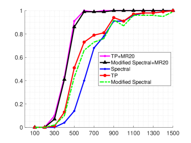
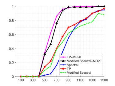
In the first experiment, we fix the dimension and choose . For each , we vary the sample size from to . We compare our algorithms with the spectral method. Since we are only interested in the initialization behavior, we shall fix the algorithm in the refinement stage to be HTP [11] as described in Algorithm 3. The results are displayed in Figure 1.
From Figure 1, we can see the TP has overall the best performance. In particular, when the sample size is insufficient, both Modified Spectral and TP have a higher chance of recovering the signal. Moreover, in both Modified Spectral and TP, the multiple-restarted version significantly increases the likelihood of successful recovery. The ability to insert the multiple-restarted step can be also regarded as an advantage of Modified Spectral and TP over Spectral. It is also clearly seen from Figure 1 that TP outperforms Modified Spectral with or without multiple restarts, which is also consistent with our theoretical result.
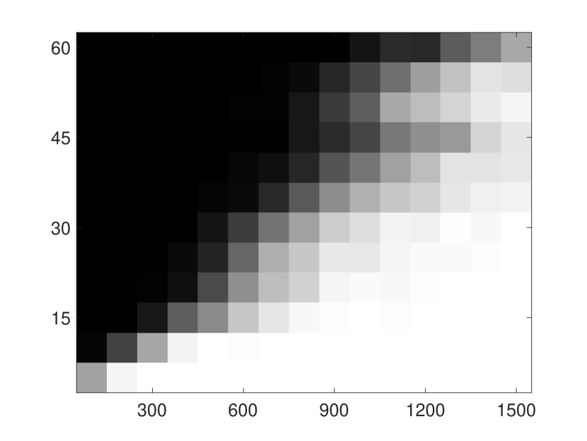
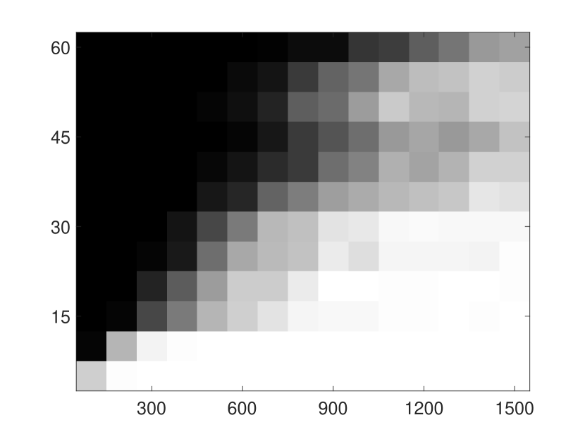
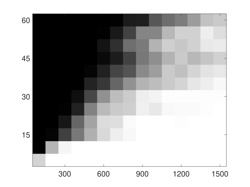
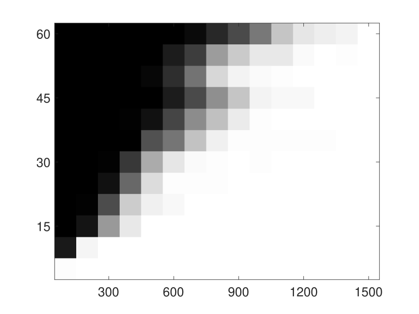
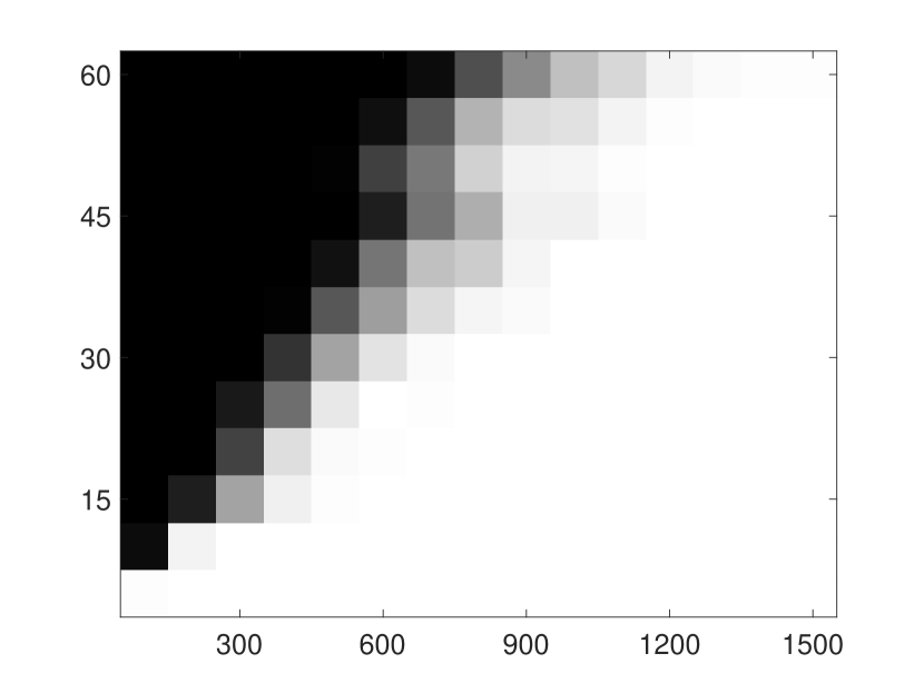
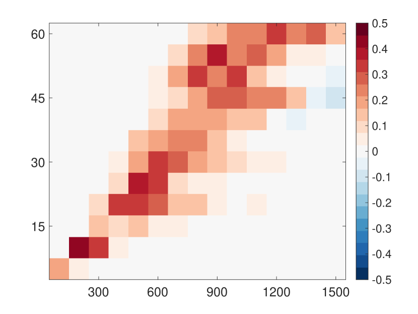
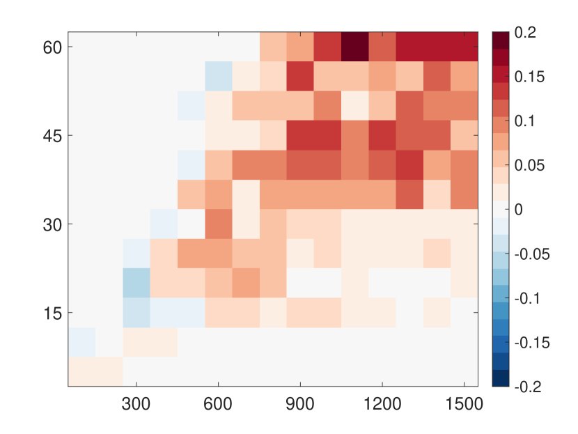
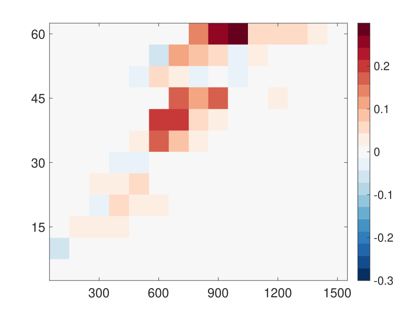
In the second experiment, we compare the phase transition of different initialization methods. Same as in the previous experiment, to have a fair comparison of different initialization algorithms, we fix the algorithm in the refinement stage to be HTP. We fix the dimension . We vary the sparsity from 5 to 60 and the sampling number from to . For TP and Modified Spectral, we also implemented their multiple-restarted versions. The results are shown in Fig. 2 and Fig. 3. We see from the figures that TP and Modified Spectral have noticeably higher rates of successful recovery than Spectral. Moreover, multiple restarts can significantly increase the chance of successful recovery. To illustrate the superiority of TP over the other two methods more clearly, we plot in Figure 4 the differences in successful recovery rates between TP and Spectral and between TP and Modified Spectral, respectively. We see that TP has a higher successful recovery rate than the other two methods, especially when is on the margin of the phase transition curve.
6 Conclusion
In this work, we have proposed two initialization algorithms for two-stage non-convex sparse phase retrieval approaches. While the popular spectral initialization requires measurements for the desired initialization, the theoretical sample complexity of our proposed algorithms is only unconditionally. Numerical simulations are provided to verify the sample efficiency of the proposed method.
References
References
- [1] S. Bahmani and J. Romberg. Efficient compressive phase retrieval with constrained sensing vectors. Advances in Neural Information Processing Systems, 28, 2015.
- [2] S. Bahmani, J. Romberg, et al. A flexible convex relaxation for phase retrieval. Electronic Journal of Statistics, 11(2):5254–5281, 2017.
- [3] S. Balakrishnan, S. S. Du, J. Li, and A. Singh. Computationally efficient robust sparse estimation in high dimensions. In Conference on Learning Theory, pages 169–212. PMLR, 2017.
- [4] R. Balan, P. Casazza, and D. Edidin. On signal reconstruction without phase. Applied and Computational Harmonic Analysis, 20(3):345–356, 2006.
- [5] Q. Berthet and P. Rigollet. Complexity theoretic lower bounds for sparse principal component detection. In Conference on learning theory, pages 1046–1066. PMLR, 2013.
- [6] J.-F. Cai, M. Huang, D. Li, and Y. Wang. The global landscape of phase retrieval I: Perturbed amplitude models. Annals of Applied Mathematics, 37(4):437–512, 2021.
- [7] J.-F. Cai, M. Huang, D. Li, and Y. Wang. The global landscape of phase retrieval II: quotient intensity models. Annals of Applied Mathematics, 38(1):62–114, 2022.
- [8] J.-F. Cai, M. Huang, D. Li, and Y. Wang. Nearly optimal bounds for the global geometric landscape of phase retrieval. arXiv preprint arXiv:2204.09416, 2022.
- [9] J.-F. Cai, M. Huang, D. Li, and Y. Wang. Solving phase retrieval with random initial guess is nearly as good as by spectral initialization. Applied and Computational Harmonic Analysis, 58:60–84, 2022.
- [10] J.-F. Cai, Y. Jiao, X. Lu, and J. You. Sample-efficient sparse phase retrieval via stochastic alternating minimization. IEEE Transactions on Signal Processing, 2022.
- [11] J.-F. Cai, J. Li, X. Lu, and J. You. Sparse signal recovery from phaseless measurements via hard thresholding pursuit. Applied and Computational Harmonic Analysis, 56:367–390, 2022.
- [12] J.-F. Cai, J. Li, and D. Xia. Generalized low-rank plus sparse tensor estimation by fast Riemannian optimization. Journal of the American Statistical Association, pages 1–17, 2022.
- [13] J.-F. Cai and K. Wei. Solving systems of phaseless equations via Riemannian optimization with optimal sampling complexity. Journal of Computational Mathematics, to appear.
- [14] T. T. Cai, X. Li, and Z. Ma. Optimal rates of convergence for noisy sparse phase retrieval via thresholded wirtinger flow. The Annals of Statistics, 44(5):2221–2251, 2016.
- [15] E. J. Candes, Y. C. Eldar, T. Strohmer, and V. Voroninski. Phase retrieval via matrix completion. SIAM review, 57(2):225–251, 2015.
- [16] E. J. Candes, X. Li, and M. Soltanolkotabi. Phase retrieval via wirtinger flow: Theory and algorithms. IEEE Transactions on Information Theory, 61(4):1985–2007, 2015.
- [17] Y. Chen and E. J. Candès. Solving random quadratic systems of equations is nearly as easy as solving linear systems. Communications on Pure and Applied Mathematics, 70(5):822–883, 2017.
- [18] Y. Chen, Y. Chi, and A. J. Goldsmith. Exact and stable covariance estimation from quadratic sampling via convex programming. IEEE Transactions on Information Theory, 61(7):4034–4059, 2015.
- [19] J. R. Fienup. Phase retrieval algorithms: a comparison. Applied Optics, 21(15):2758–2769, 1982.
- [20] T. Goldstein and C. Studer. Phasemax: Convex phase retrieval via basis pursuit. IEEE Transactions on Information Theory, 64(4):2675–2689, 2018.
- [21] P. Hand and V. Voroninski. An elementary proof of convex phase retrieval in the natural parameter space via the linear program phasemax. Communications in Mathematical Sciences, 16(7):2047–2051, 2018.
- [22] R. W. Harrison. Phase problem in crystallography. JOSA a, 10(5):1046–1055, 1993.
- [23] R. A. Horn and C. R. Johnson. Matrix analysis. Cambridge university press, 2012.
- [24] M. Iwen, A. Viswanathan, and Y. Wang. Robust sparse phase retrieval made easy. Applied and Computational Harmonic Analysis, 42(1):135–142, 2017.
- [25] G. Jagatap and C. Hegde. Sample-efficient algorithms for recovering structured signals from magnitude-only measurements. IEEE Transactions on Information Theory, 65(7):4434–4456, 2019.
- [26] M. Journée, Y. Nesterov, P. Richtárik, and R. Sepulchre. Generalized power method for sparse principal component analysis. Journal of Machine Learning Research, 11(2), 2010.
- [27] B. Laurent and P. Massart. Adaptive estimation of a quadratic functional by model selection. Annals of Statistics, pages 1302–1338, 2000.
- [28] Z. Li, J. Cai, and K. Wei. Toward the optimal construction of a loss function without spurious local minima for solving quadratic equations. IEEE Transactions on Information Theory, 66(5):3242–3260, 2020.
- [29] Z. Liu, S. Ghosh, and J. Scarlett. Towards sample-optimal compressive phase retrieval with sparse and generative priors. Advances in Neural Information Processing Systems, 34:17656–17668, 2021.
- [30] W. Luo, W. Alghamdi, and Y. M. Lu. Optimal spectral initialization for signal recovery with applications to phase retrieval. IEEE Transactions on Signal Processing, 67(9):2347–2356, 2019.
- [31] C. Ma, K. Wang, Y. Chi, and Y. Chen. Implicit regularization in nonconvex statistical estimation: Gradient descent converges linearly for phase retrieval and matrix completion. In International Conference on Machine Learning, pages 3345–3354. PMLR, 2018.
- [32] Z. Ma. Sparse principal component analysis and iterative thresholding. The Annals of Statistics, 41(2):772–801, 2013.
- [33] S. Mallat. A wavelet tour of signal processing. Academic Press, 1998.
- [34] J. Miao, T. Ishikawa, Q. Shen, and T. Earnest. Extending x-ray crystallography to allow the imaging of noncrystalline materials, cells, and single protein complexes. Annu. Rev. Phys. Chem., 59:387–410, 2008.
- [35] B. Moghaddam, Y. Weiss, and S. Avidan. Spectral bounds for sparse pca: Exact and greedy algorithms. Advances in neural information processing systems, 18, 2005.
- [36] M. Mondelli and A. Montanari. Fundamental limits of weak recovery with applications to phase retrieval. Foundations of Computational Mathematics, 19(3), 2019.
- [37] P. Netrapalli, P. Jain, and S. Sanghavi. Phase retrieval using alternating minimization. In Advances in Neural Information Processing Systems, pages 2796–2804, 2013.
- [38] P. Netrapalli, P. Jain, and S. Sanghavi. Phase retrieval using alternating minimization. IEEE Transactions on Signal Processing, 63(18):4814–4826, 2015.
- [39] F. Salehi, E. Abbasi, and B. Hassibi. Learning without the phase: Regularized phasemax achieves optimal sample complexity. Advances in Neural Information Processing Systems, 31, 2018.
- [40] Y. Shechtman, Y. C. Eldar, O. Cohen, H. N. Chapman, J. Miao, and M. Segev. Phase retrieval with application to optical imaging: a contemporary overview. IEEE Signal Processing Magazine, 32(3):87–109, 2015.
- [41] Y. Shen, J. Li, J.-F. Cai, and D. Xia. Computationally efficient and statistically optimal robust low-rank matrix estimation. arXiv preprint arXiv:2203.00953, 2022.
- [42] M. Soltanolkotabi. Structured signal recovery from quadratic measurements: Breaking sample complexity barriers via nonconvex optimization. IEEE Transactions on Information Theory, 65(4):2374–2400, 2019.
- [43] J. Sun, Q. Qu, and J. Wright. A geometric analysis of phase retrieval. Foundations of Computational Mathematics, 18(5):1131–1198, 2018.
- [44] T. Tong, C. Ma, and Y. Chi. Accelerating ill-conditioned low-rank matrix estimation via scaled gradient descent. J. Mach. Learn. Res., 22:150–1, 2021.
- [45] T. Tong, C. Ma, A. Prater-Bennette, E. Tripp, and Y. Chi. Scaling and scalability: Provable nonconvex low-rank tensor estimation from incomplete measurements. Journal of Machine Learning Research, 23(163):1–77, 2022.
- [46] R. Vershynin. High-dimensional probability: An introduction with applications in data science, volume 47. Cambridge university press, 2018.
- [47] I. Waldspurger, A. d’Aspremont, and S. Mallat. Phase recovery, maxcut and complex semidefinite programming. Mathematical Programming, 149(1):47–81, 2015.
- [48] A. Walther. The question of phase retrieval in optics. Journal of Modern Optics, 10(1):41–49, 1963.
- [49] G. Wang and G. Giannakis. Solving random systems of quadratic equations via truncated generalized gradient flow. In Advances in Neural Information Processing Systems, pages 568–576, 2016.
- [50] G. Wang, L. Zhang, G. B. Giannakis, M. Akakaya, and J. Chen. Sparse phase retrieval via truncated amplitude flow. IEEE Transactions on Signal Processing, 66(2):479–491, 2017.
- [51] Y. Wang and Z. Xu. Phase retrieval for sparse signals. Applied and Computational Harmonic Analysis, 37(3):531–544, 2014.
- [52] K. Wei, J.-F. Cai, T. F. Chan, and S. Leung. Guarantees of Riemannian optimization for low rank matrix recovery. SIAM Journal on Matrix Analysis and Applications, 37(3):1198–1222, 2016.
- [53] F. Wu and P. Rebeschini. Hadamard wirtinger flow for sparse phase retrieval. In International Conference on Artificial Intelligence and Statistics, pages 982–990. PMLR, 2021.
- [54] X.-T. Yuan and T. Zhang. Truncated power method for sparse eigenvalue problems. Journal of Machine Learning Research, 14(4), 2013.
- [55] H. Zhang and Y. Liang. Reshaped wirtinger flow for solving quadratic system of equations. In Advances in Neural Information Processing Systems, pages 2622–2630, 2016.