Eigenstate thermalization hypothesis in two-dimensional XXZ model with or without SU(2) symmetry

Abstract

We investigate the eigenstate thermalization properties of the spin-1/2 XXZ model in two-dimensional rectangular lattices of size $L_{1}\times L_{2}$ under periodic boundary conditions. Exploiting the symmetry property, we can perform an exact diagonalization study of the energy eigenvalues up to system size $4\times 7$ and of the energy eigenstates up to $4\times 6$. Numerical analysis of the Hamiltonian eigenvalue spectrum and matrix elements of an observable in the Hamiltonian eigenstate basis supports that the two-dimensional XXZ model follows the eigenstate thermalization hypothesis. When the spin interaction is isotropic the XXZ model Hamiltonian conserves the total spin and has SU(2) symmetry. We show that the eigenstate thermalization hypothesis is still valid within each subspace where the total spin is a good quantum number.

I Introduction

The eigenstate thermalization hypothesis (ETH) explains the mechanism for thermalization of isolated quantum systems [1, 2]. The ETH guarantees that a quantum mechanical expectation value of a local observable relaxes to the equilibrium ensemble averaged value and fluctuations in the steady state satisfy the fluctuation dissipation theorem (see Ref. [3] and references therein).

Numerous studies have been performed to test validity of the ETH since the early work of Ref. [4]. The spin-1/2 XXZ model [5, 6, 7, 8, 9, 10, 11, 12, 13, 14] and the quantum Ising spin model [7, 15, 16, 17, 18] are the paradigmatic model systems for ETH study. The XXZ model is useful since it describes a hardcore boson system which is relevant to experimental ultracold atom systems [19, 20, 21, 22, 23]. Moreover, integrability in these models can be tuned easily in one-dimensional lattices. A thermal/nonthermal behavior and a crossover between them have been studied comprehensively using the model systems [24, 5, 25, 26, 6, 27, 7, 28, 11, 29, 30].

The ETH has been examined mostly in one-dimensional spin systems, and there are only a few works for two-dimensional systems [4, 16, 17, 15, 31]. In this work, we study the eigenstate thermalization property of the spin-1/2 XXZ model in two-dimensional rectangular lattices. In comparison with the Ising spin systems [15, 16, 17], the XXZ model is characterized by the conservation of the magnetization in the $z$ direction. Furthermore, it possesses the SU(2) symmetry when the spin interaction is isotropic [32]. The SU(2) symmetry conserves the magnetization in all directions, but the total spin operators in different directions do not commute with each other. Such a non-Abelian symmetry has a nontrivial effect on many-body localization [33, 34], quantum thermalization [35, 32, 36], and entanglement entropy [37].

This paper is organized as follows. In Sec. II, we introduce the XXZ Hamiltonian with nearest and next nearest neighbor interactions in two-dimensional rectangular lattices. The symmetry property of the Hamiltonian is summarized. In Secs. III and IV, we present results of a numerical exact diagonalization study. First, we will show in Sec. III that the ETH is valid in the XXZ model without SU(2) symmetry. In Sec. IV, we proceed to show that the SU(2) symmetric XXZ model also satisfies the ETH in each SU(2) subsector. Our work extends the validity of the ETH to the two-dimensional XXZ model.

II Two-dimensional XXZ model

We consider the spin-1/2 XXZ model on a two-dimensional rectangular lattice. The Pauli spin $\bm{\sigma}_{\bm{r}}=(\sigma^{x}_{\bm{r}},\sigma^{y}_{\bm{r}},\sigma^{z}_{\bm{r}})$ resides on a lattice site ${\bm{r}}$ and the Hamiltonian is given by

$$H=\lambda\sum_{\langle\bm{r},\bm{r^{\prime}}\rangle}h(\bm{\sigma}_{\bm{r}},\bm{\sigma_{\bm{r}^{\prime}}})+(1-\lambda)\sum_{[\bm{r},\bm{r^{\prime}}]}h(\bm{\sigma}_{\bm{r}},\bm{\sigma_{\bm{r}^{\prime}}}),$$ (1)

where $\langle\bm{r},\bm{r^{\prime}}\rangle$ and $[\bm{r},\bm{r^{\prime}}]$ denote the pair of nearest neighbor (nn) sites, connected by solid lines in Fig. 1(a), and of next nearest neighbor (nnn) sites, connected by dotted lines in Fig. 1(a), respectively, and $h(\bm{\sigma},\bm{\sigma_{r^{\prime}}})$ denotes the XXZ coupling given by

$$h(\bm{\sigma_{r}},\bm{\sigma_{r^{\prime}}})=-\frac{J}{2}\left(\sigma^{x}_{\bm{r}}\sigma^{x}_{\bm{r}^{\prime}}+\sigma^{y}_{\bm{r}}\sigma^{y}_{\bm{r}^{\prime}}+\Delta\sigma^{z}_{\bm{r}}\sigma^{z}_{\bm{r}^{\prime}}\right).$$ (2)

The model is defined by three parameters $J$, $\Delta$, and $\lambda$: $\lambda$ controls the relative strength of the nn and nnn couplings, $\Delta$ is an anisotropy parameter, and $J$ sets the overall energy scale which will be kept to be 1. We assume periodic boundary conditions, $\bm{\sigma}_{{\bm{r}}+L_{1}{\bm{e}}_{1}}=\bm{\sigma}_{{\bm{r}}+L_{2}{\bm{e}_{2}}}=\bm{\sigma}_{\bm{r}}$ where $\bm{e}_{1}$ and $\bm{e}_{2}$ are the unit vectors in the horizontal and vertical directions, respectively [see Fig. 1(a)]. The XXZ coupling with $J=1$ can be rewritten as

$$h(\bm{\sigma_{r}},\bm{\sigma_{r^{\prime}}})=-\left(\sigma^{+}_{\bm{r}}\sigma^{-}_{\bm{r}^{\prime}}+\sigma^{-}_{\bm{r}}\sigma^{+}_{\bm{r}^{\prime}}+\frac{\Delta}{2}\sigma^{z}_{\bm{r}}\sigma^{z}_{\bm{r}^{\prime}}\right)$$ (3)

with the raising and lowering operators $\sigma^{\pm}\equiv(\sigma^{x}\pm i\sigma_{y})/2$. Throughout the paper, we will set $\hbar=1$. The total number of sites will be denoted by $N=L_{1}L_{2}$. In this work, we only consider the lattices with even $N$.

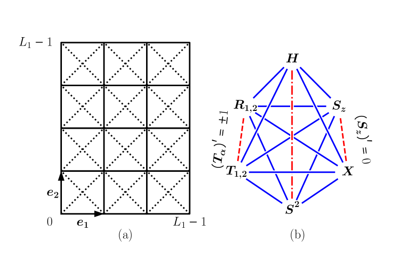
Figure 1: (a) Rectangular lattice of size $L_{1}\times L_{2}$ under periodic boundary conditions in the horizontal ($\bm{e}_{1}$) and vertical ($\bm{e}_{2}$) directions. (b) Commutation relations among the XXZ Hamiltonian and symmetry operators. Mutually commuting operators are connected with a solid line. A dashed line connect operators which are commuting only within the subspace with specific quantum numbers of the symmetry operator. The Hamiltonian and $\bm{S}^{2}$, connected by a dashed-dotted line, commutes only when $\Delta=1$.

The XXZ Hamiltonian commutes with several symmetry operators. First, the Hamiltonian commutes with the magnetization operator in the $z$ direction

$$S_{z}=\frac{1}{2}\sum_{\bm{r}}\sigma^{z}_{\bm{r}}.$$ (4)

The Hamiltonian also commutes with the shift operator $T_{\alpha}$ which shifts a spin state by the unit distance in the direction ${\bm{e}}_{\alpha}$ with $\alpha=1,2$:

$$T^{-1}_{\alpha}\bm{\sigma_{r}}T_{\alpha}=\bm{\sigma}_{{\bm{r}}+{\bm{e}}_{\alpha}}\quad(\alpha={1},{2}).$$ (5)

The system has the spatial inversion symmetry so that $H$ commutes with $R_{\alpha}$ which maps a site $\bm{r}=(x,y)$ to $(-x,y)$ for ${\alpha}=1$ or to $(x,-y)$ for ${\alpha}=2$. Finally, the system is invariant under the spin flip $\sigma^{z}\to-\sigma^{z}$ which is generated by the symmetry operator $X=\prod_{{\bm{r}}}\sigma^{x}_{\bm{r}}$.

The commutation relations are summarized by a diagram in Fig. 1(b). (A similar diagram for the one-dimensional system is found in Ref. [38].) Note that $[X,S_{z}]\neq 0$ and $[R_{\alpha},T_{\alpha}]\neq 0$ in general. Thus, one cannot construct a simultaneous basis set for all the symmetry operators. On the other hand, one can show that $[R_{\alpha},T_{\alpha}]|\psi\rangle=0$ if a state $|\psi\rangle$ is an eigenstate of $T_{\alpha}$ of eigenvalue $(T_{\alpha})^{\prime}=\pm 1$. It implies that the two operators commute within the subspace of the eigenstates of $T_{\alpha}$ with eigenvalues $\pm 1$, Likewise, $[X,S_{z}]=0$ within the subspace of the eigenstates of $S_{z}$ with eigenvalue $(S_{z})^{\prime}=0$. In this work, we focus on the symmetry sector consisting of the eigenvalues of the symmetry operators with the eigenvalues $(T_{\alpha})^{\prime}=(R_{\alpha})^{\prime}=(X)^{\prime}=1$ and $(S_{z})^{\prime}=0$, which will be referred to as the maximum symmetry sector (MSS).

When the spin-spin interaction is isotropic ($\Delta=1$), the Hamiltonian is invariant under spin rotation [SU(2) symmetry]. Consequently, each component of the total spin $\bm{S}=\frac{1}{2}\sum_{\bm{r}}\bm{\sigma_{r}}$ is conserved and $\bm{S}^{2}=\bm{S}\cdot\bm{S}$ becomes the symmetry operator commuting with the Hamiltonian and all the other symmetry operators. The maximum symmetry sector is then further decomposed into subsectors characterized with the eigenvalue of $\bm{S}^{2}$, $(\bm{S}^{2})^{\prime}=s(s+1)$ with integer $s$. The SU(2) symmetry will be investigated in detail in Sec. IV.

We have performed the exact diagonalization study. The basis states, which are simultaneous eigenstates of the symmetry operators appearing in Fig. 1(b) in the MSS, can be easily constructed using the methods summarized in Refs. [39, 40, 41, 42, 43, 38]. The Hilbert space dimensionalities of the MSS are $D=26$, $1392$, $15578$, and $183926$ when $L_{1}\times L_{2}=4\times 3$, $4\times 5$, $4\times 6$, $4\times 7$, respectively. When $L_{1}=L_{2}$, the system has an addition symmetry under the spatial rotation by a multiple of $\pi/2$. It will not be addressed since we only consider the lattices with $L_{1}\neq L_{2}$.

An energy eigenstate and a corresponding eigenvalue of $H$ in the MSS will be denoted as $|E_{n}\rangle$ and $E_{n}$, respectively, where the quantum number $n=0,\cdots,D-1$ is assigned in ascending order of the energy eigenvalue. We will study the Hamiltonian spectrum and the matrix elements of the observable,

$$\begin{split}O^{Z}&=\frac{1}{N}\sum_{\bm{r}}\sum_{\alpha=1,2}\sigma_{\bm{r}}^{z}\sigma_{\bm{r}+\bm{e}_{\alpha}}^{z}\\ O^{J}&=\frac{1}{N}\sum_{\bm{r}}\sum_{{\alpha}=1,2}\left(\sigma_{\bm{r}}^{+}\sigma_{\bm{r}+\bm{e}_{\alpha}}^{-}+\sigma_{\bm{r}+\bm{e}_{\alpha}}^{+}\sigma_{\bm{r}}^{-}\right)\\ O^{P}&=\frac{1}{N}\sum_{\bm{r},\bm{r^{\prime}}}\sigma_{\bm{r}}^{+}\sigma_{\bm{r^{\prime}}}^{-}\\ O^{F}&=\frac{1}{N}\sum_{p}\sigma_{p_{1}}^{z}\sigma_{p_{2}}^{z}\sigma_{p_{3}}^{z}\sigma_{p_{4}}^{z},\end{split}$$ (6)

which measure the nearest neighbor two-spins correlation, nearest neighbor hopping amplitude, zero-momentum distribution function, and the plaquette interaction of four spins. The sum in $O^{F}$ is over all plaquettes and $\sigma_{p_{i}}$ ($i=1,2,3,4$) refers to four spins around a plaquette $p$.

III Numerical study of eigenstate thermalization hypothesis

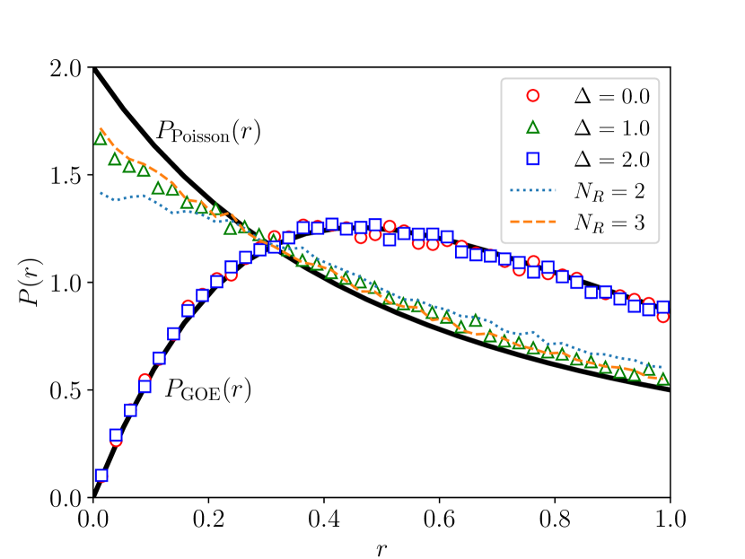
Figure 2: Distributions of the ratio of consecutive energy gaps of the XXZ model with $\lambda=1$ on the rectangular lattice of size $4\times 7$. These data are obtained from the half of the energy eigenvalues in the middle of the entire spectrum. They are compared with the corresponding distribution from the Poisson-distributed energy spectrum, $P_{\rm Poisson}(r)$, and the random matrix spectrum in the Gaussian orthogonal ensemble, $P_{\rm GOE}(r)$. The peculiar shape of the distribution at $\Delta=1$ is ascribed to the SU(2) symmetry, which will be analyzed in detail in Sec. IV. The dotted and dashed lines are from a mixture of replicated spectra, which will be also explained in Sec. IV.

III.1 Ratio of consecutive energy gaps

As a signature for the quantum chaos, we investigate the statistics of the ratio of consecutive energy gaps [44, 45]:

$$r_{n}=\min\left[\frac{E_{n+1}-E_{n}}{E_{n}-E_{n-1}},\frac{E_{n}-E_{n-1}}{E_{n+1}-E_{n}}\right].$$ (7)

Figure 2 shows the numerical data obtained with the parameters $\Delta=0,1$, and $2$ with fixed $\lambda=1$. When $\Delta=0$ and $2$, the distribution is in good agreement with the distribution function

$$P_{\rm GOE}(r)=\frac{27}{4}\frac{(r+r^{2})}{(1+r+r^{2})^{5/2}},$$ (8)

which describes the distribution for random matrices in the Gaussian orthogonal ensemble (GOE) [45]. The agreement implies that the XXZ model is quantum chaotic at $\lambda=1$. We also confirmed the quantum-chaotic behavior at $\lambda=1/2$, which is not shown.

The one-dimensional XXZ model with $\Delta=0$ and $\lambda=1$ is mapped to the free fermion model via the Jordan-Wigner transformation [46], thus it is integrable. The transformation, however, generates nonlocal interaction terms for a two-dimensional system. Thus, the two-dimensional XXZ model is nonintegrable even when $\Delta=0$.

At $\Delta=1$, the distribution deviates significantly from $P_{\rm GOE}(r)$. It also deviates from $P_{\rm Poisson}(r)=2/(1+r)^{2}$, which is characteristic of a nonchaotic system following the Poisson statistics [45]. At $\Delta=1$, the system is SU(2) symmetric and the energy eigenvalue spectrum in the MSS is a mixture of the spectrum from all the SU(2) subsectors, which results in a deviation from the GOE distribution [47]. We will scrutinize the role of the SU(2) symmetry in Sec. IV.

III.2 Statistics of diagonal elements

The ETH proposes that matrix elements of an observable $O$, $O_{mn}\equiv\langle E_{m}|O|E_{n}\rangle$, take the form

$$O_{mn}=g_{O}(E_{mn})\delta_{mn}+\frac{e^{-S(E_{mn})/2}}{{N}^{\theta}}f_{O}(E_{mn},\omega_{mn})R_{mn},$$ (9)

where $E_{mn}=(E_{m}+E_{n})/2$, $\omega_{mn}=(E_{m}-E_{n})$, $S(E)$ is the thermodynamic entropy (the Boltzmann constant is set to unity), $g_{O}$ and $f_{O}$ are smooth functions of their arguments, and $\{R_{mn}\}$ are fluctuating variables having the statistical properties similar to elements of a random matrix in the GOE [1, 2, 3]. The ETH ansatz applies to an operator whose Hilbert-Schmidt norm is normalized to an $O(1)$ constant [14]. The factor ${N}^{-\theta}$ is included in Eq. (9) as a compensation for the Hilbert-Schmidt norm of the operators in Eq. (6). Specifically, $\theta=1/2$ for $O^{Z,J,F}$ and $\theta=0$ for $O^{P}$ [48, 49]. This ansatz guarantees the quantum thermalization and the fluctuation-dissipation theorem for isolated quantum systems [3, 50, 51, 52, 53, 12, 14]. Note that the quantities $R_{mn}$ follow a Gaussian distribution as the random matrix elements in the GOE. We remark, however, that their higher order correlations are not described by the GOE random matrix theory [54, 55, 56, 57, 58, 59, 60]. In this work, we focus on the Gaussian nature of the distribution and do not study the higher order correlations.

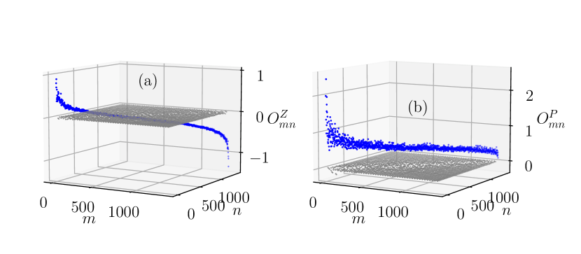
Figure 3: Matrix elements $O^{Z}_{mn}$ in (a) and $O^{P}_{mn}$ in (b) in the Hamiltonian eigenstate basis with $m,n=0,\cdots,1391$. The lattice size is $4\times 5$ and model parameters are $\Delta=2$ and $\lambda=1$.

Figure 3 presents matrix elements of $O^{Z}$ and $O^{P}$. Diagonal elements, far from the spectrum edges, vary smoothly with the energy quantum number. Offdiagonal elements have a relatively smaller magnitude than diagonal elements. These overall features are consistent with the ETH ansatz.

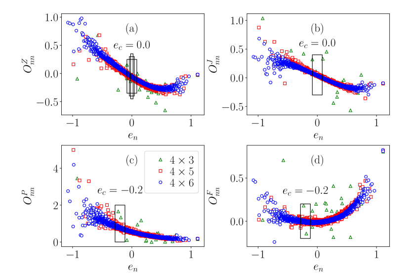
Figure 4: Diagonal matrix elements $O_{nn}=\langle E_{n}|O|E_{n}\rangle$ versus energy density $e_{n}=E_{n}/{N}$ at three different lattice sizes with $\Delta=2$ and $\lambda=1/2$. Rectangular boxes represent energy windows $W(e_{c}N,\delta E)$ of width $\delta E=0.5,1.0,2.0$ for $O^{Z}$ and $\delta E=2.0$ for the other observables for the system of size $4\times 6$.

The diagonal elements are plotted in Fig. 4. According to the ETH, diagonal elements $O_{nn}$ should follow the Gaussian distribution with mean $g_{O}(E_{n})$ and variance $e^{-S(E_{n})}|f_{O}(E_{n},0)|^{2}$. This ansatz can be tested with the distribution of the diagonal elements for energy eigenstates in an energy window $W(E_{c},\delta E)$, a set of energy eigenstate whose energy eigenvalues lie within an interval $E_{c}-\delta E\leq E_{n}\leq E_{c}+\delta E$. Rectangular boxes drawn in Fig. 4(a) represent the energy windows of width $\delta E=0.5,1,$ and $2$ with $e_{c}=E_{c}/N=0.0$. The distribution of the diagonal elements within an energy window is influenced by two factors [61, 49]: (i) intrinsic eigenstate-to-eigenstate fluctuations and (ii) extrinsic fluctuations due to a systematic energy dependence of the diagonal elements. It is clear that the extrinsic fluctuations become dominant as $\delta E$ increases.

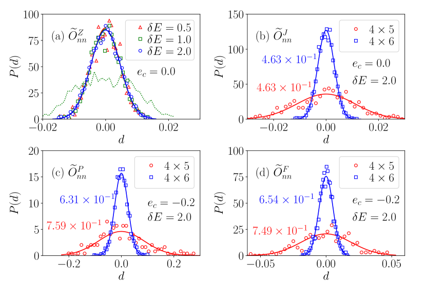
Figure 5: Distribution of detrended diagonal matrix elements $d=\widetilde{O}_{nn}$ within the energy window $W(E_{c}=e_{c}N,\delta E)$ depicted with the rectangular boxes in Fig. 4. Model parameters are $\Delta=2$ and $\lambda=1/2$. (a) We compare the distributions for the operator $O^{Z}$ with the choice of three different values $\delta E$ when the lattice is of size $4\times 6$. The solid curves represent the Gaussian distribution of the same mean and variance as the histogram data. The dotted line is the probability distribution of the bare diagonal elements, after being subtracted by their mean value, with $\delta E=1.0$. (b)-(d) We compare the distributions obtained from the lattices of size $4\times 5$ and $4\times 6$. All the distributions are consistent with the Gaussian distributions (solid curves). Numerical values of $\sigma_{d}^{2}N^{2\theta}D$ (see main text) are annotated in (b)-(d).

In order to reduce a finite $\delta E$ effect and isolate the intrinsic fluctuations, we introduce a detrended diagonal element [61]

$$\widetilde{O}_{nn}=O_{nn}-h_{W}(E_{n}),$$ (10)

where $h_{W}(E)$ is a fitting function to $O_{nn}$ within an energy window $W(E_{c},\delta E)$. In this work, we choose a linear function for $h_{W}(E)$. In Fig. 5(a), we compare the distributions of the detrended diagonal elements of $O^{Z}$ with three different values of $\delta E=0.5,1.0$, and $2.0$. Those distributions are almost identical to each other, which implies that the detrending removes the extrinsic fluctuations. We also present the distribution of the bare diagonal elements within the energy window of width $\delta E=1$. They are shifted to have zero mean. The bare distribution is much broader than the detrended distribution due to the extrinsic fluctuations. This comparison demonstrates that the detrending is useful. It allows one to take a large value of $\delta E$ for better statistics without suffering from the finite $\delta E$ effect. In Figs. 5(b)-(d), we present the distributions of the detrended diagonal elements of the observables $O^{J}$, $O^{P}$, and $O^{F}$ within the energy windows shown in Figs. 4(b)-(d). The numerical results are in good agreement with the Gaussian distributions of the same mean and variance, which supports the ETH.

According to the ETH in Eq. (9), the variance of the diagonal elements $\sigma_{d}^{2}$ normalized with the system size, $\sigma^{2}_{d}N^{2\theta}$, should be inversely proportional to the density of states $D\simeq|W(e_{c}N,\delta E)|/\delta E=e^{S(e_{c}N)}$. This scaling law can be checked by using a plot of $\sigma^{2}_{d}N^{2\theta}$ against $D^{-1}$ for more than three different system sizes, as was done in Ref. [13]. In the current work, numerical data are available from only two different system sizes $4\times 5$ and $4\times 6$. Due to the limited range of system sizes, we cannot perform such a systematic finite size scaling analysis. Alternatively, we only report the quantitative values of $\sigma_{d}^{2}N^{2\theta}D$. The numerical values at two different system sizes, shown in Figs. 5(b)-(d), are close to each other up to a relative error of $\lesssim 15\%$, which supports the scaling behavior $\sigma_{d}^{2}N^{2\theta}\propto 1/D$.

III.3 Statistics of off diagonal elements

We also investigate the statistical property of the offdiagonal elements $o=O_{mn}$ for $|E_{n}\rangle$ and $|E_{m}\rangle\in W(E_{c}=e_{c}N,\delta E)$ with $n\neq m$. These offdiagonal elements correspond to the term $\frac{e^{-S(e_{c}N)}}{N^{\theta}}f_{O}(e_{c}N,\omega\simeq 0)R_{mn}$ with $m\neq n$ in the ETH ansatz of Eq. (9). Figure 6 presents the distributions for the four observables. Each numerical distribution function is in good agreement with the Gaussian distribution of the same mean and variance, which is consistent with the ETH.

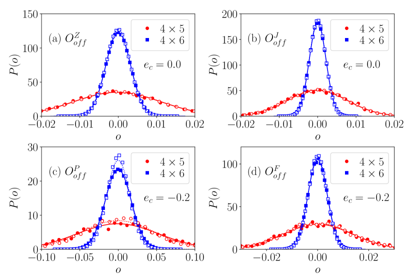
Figure 6: Distribution of offdiagonal matrix elements $O_{mn}$ with $m\neq n$ among energy eigenstates within the energy window $W(E_{c}=e_{c}N,\delta E)$ of width $\delta E=0.5$ (filled symbols and solid lines) and $\delta E=1.0$ (open symbols and dashed lines) centered at the energy density $e_{c}=0.0$ or $-0.2$. The curves represent the Gaussian distribution with the same mean and variance as the histogram data. The model parameters are $\Delta=2$ and $\lambda=1/2$.

To test the ETH further, we compare the variances $\sigma^{2}_{d}$ and $\sigma^{2}_{o}$ of the diagonal and offdiagonal elements, respectively. For each energy eigenstate $|E_{n}\rangle$, we construct an energy window $W(E_{c}=E_{n},\delta E)$, calculate the matrix elements, and evaluate a variance ratio $q_{n}=\sigma_{o}^{2}/\sigma_{d}^{2}$. The diagonal elements are detrended as explained in Sec. III.2. The ratio $q_{n}$ obtained with $\delta E=0.5$ is plotted as a function of the energy density $e_{n}=E_{n}/N$ in Fig. 7. The ratio is fluctuating around the mean value, and the amplitude of fluctuations decreases as the system size increases except for the spectrum edges. The mean value is close to $1/2$, which is also consistent with the ETH prediction.

We add a remark on a finite $\delta E$ effect. The shape of the distributions shown in Fig. 6 varies slightly with $\delta E$. According to the ETH, an offdiagonal element $O_{mn}$ is a Gaussian random variable of variance $e^{-S(E_{mn})}|f_{O}(E_{mn},\omega_{mn})|^{2}/{N}^{2\theta}$. Given a finite value of $\delta E$, the term $e^{-S(E)}|f_{O}(E,\omega)|^{2}$ may vary around a mean value $e^{-S(E_{c})}|f_{O}(E_{c},0)|^{2}$ up to $O(\delta E)$. Unlike the case for diagonal elements, the variation leads to a subleading contribution to the variance of offdiagonal elements. Thus, a finite-$\delta E$ effect is weak for the offdiagonal elements. The numerical results in Fig. 6 shows that such an effect is indeed negligible for $O^{Z}$, $O^{J}$, $O^{F}$ with $\delta E=0.5$. On the other hand, it is still noticeable for $O^{P}$ in Fig. 6(c). We attribute the result $\langle q\rangle\simeq 0.44$ in Fig. 7(c) to a finite-$\delta E$ effect.

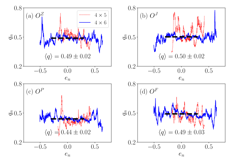
Figure 7: Variance ratio $q_{n}=\sigma_{o}^{2}/\sigma_{d}^{d}$ for the model with $\Delta=2$ and $\lambda=0.5$ and $L_{1}\times L_{2}=4\times 5$ (dotted line) and $4\times 6$ (solid line). The mean value and the standard deviation of the ratios $\{q_{n}\}$ within the energy interval $-0.3<e_{n}<0.3$ are presented in each panel (broken line) for $L_{1}\times L_{2}=4\times 6$.

IV SU(2) symmetric XXZ model with $\Delta=1$

We have shown that the XXZ model in the symmetry-resolved MSS obeys the ETH. When $\Delta=1$, the XXZ Hamiltonian has an additional symmetry under the global spin rotation, SU(2) symmetry. Thus, the MSS can be further decomposed into the symmetry subsectors, called SU(2) subsectors, each of which is characterized with the total spin quantum number $s$ as described in Sec. II. In this section, we investigate whether the ETH is also valid for the SU(2)-symmetric XXZ model.

In Fig. 2, we have seen that the distribution $P(r)$ for the ratio of consecutive energy gaps at $\Delta=1$ deviates from $P_{\rm GOE}(r)$ and $P_{\rm Poisson}(r)$. The SU(2) symmetry is responsible for it. The MSS is the union of the SU(2)-symmetric subsectors. Recently, it was found that presence of symmetry subsectors modifies the gap ratio distribution function from the universal form [47]. Even if the energy spectrum in each subsector follows the GOE statistics, $P(r)$ from the whole spectrum is characterized by a distinct form determined by the number of subsectors and their relative sizes [47].

In order to understand the shape of $P(r)$ at $\Delta=1$, we construct an artificial set of energy eigenvalues $\mathcal{E}(N_{R})$ as the union of shifted replicas of the real energy spectrum $\{E_{n}\}$ obtained at $\Delta=2$, $\mathcal{E}(N_{R})=\cup_{p=1}^{N_{R}}\{E_{n}+(p-1)\Delta E\}$ with $N_{R}$ the number of replicas. We took $\Delta E~{}(=0.1)$ which is much larger than the mean level spacing. Figure 2 shows the distribution functions of the superimposed spectrum with $N_{R}=2$ (dotted line) and $N_{R}=3$ (dashed line). These data confirm that the the distribution of the superimposed spectrum is different from $P_{\rm Poisson}$ and $P_{\rm GOE}$ [47]. We note that the distribution function $P(r)$ at $\Delta=1$ lies between the distribution functions from the superimposed energy spectrum of $N_{R}=2$ (dotted line) or $3$ (dashed line) replicas. This comparison suggests that the energy spectrum in each SU(2) subsector obeys the GOE statistics and that a few $(2\sim 3)$ SU(2) subsectors are dominant in the MSS.

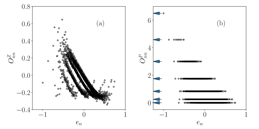
Figure 8: Diagonal elements of the operators $O^{Z}$ and $O^{P}$ in the energy eigenstate basis when $\Delta=1$, $\lambda=1/2$, and $L_{1}\times L_{2}=4\times 6$. Note that the diagonal elements of $O^{P}$ are quantized to the values $s(s+1)/N$ with $N=24$ and $s=0,2,\cdots,12$ as indicated by arrows.

Figure 8 shows the diagonal elements of the operators $O^{Z}$ and $O^{P}$ in the energy eigenstate basis at the SU(2) symmetric point ($\Delta=1$ and $\lambda=1/2$). One finds that the diagonal elements are organized into several branches. Moreover, the diagonal elements of $O^{P}$ are quantized. Note that $O^{P}$ defined in Eq. (6) is rewritten as

$$O^{P}=S^{+}S^{-}/N=(\bm{S}^{2}-(S^{z})^{2}+S^{z})/N$$ (11)

in terms of the total spin operator $\bm{S}=\frac{1}{2}\sum_{\bm{r}}\bm{\sigma}_{\bm{r}}$. Thus, the diagonal element of $O^{P}$ in the MSS [$(S^{z})^{\prime}=0$] takes a quantized value

$$\langle E_{n}|O^{P}|E_{n}\rangle=s_{n}(s_{n}+1)/N$$ (12)

with a nonnegative integer $s_{n}$ equal to or less than $s_{max}=N/2$. Since $N=L_{1}L_{2}$ is even in this work, the total spin quantum number takes an integral value.

Figure 9: Diagonal elements of the operators (a) $O^{Z}$ and (b) $O^{J}$ when $\Delta=1$, $\lambda=1/2$, and $L_{1}\times L_{2}=4\times 6$. Diagonal elements are plotted with different symbols depending on their total spin quantum number $s$. The inset in (b) shows $D_{s}$, the number of eigenstates in the SU(2) subsector of total spin quantum number $s$.

Using the quantization in Eq. (12), one can identify the total spin quantum number $s$ of an energy eigenstate. We present the diagonal elements of $O^{Z}$ and $O^{J}$ in each SU(2) subsector in Fig. 9. It is clear that the branch corresponds to the SU(2) subsector. Note that the SU(2) subsectors with odd $s$ are missing. An odd $s$ is not compatible with the other symmetries in the MSS.

Before proceeding further, we briefly review the theory of spin addition. Consider two spins $\bm{S}_{1}$ and $\bm{S}_{2}$ with $(\bm{S}_{1,2}^{2})^{\prime}=s_{1,2}(s_{1,2}+1)$. The sum of them $\bm{S}=\bm{S}_{1}+\bm{S}_{2}$ has an eigenvalue $(\bm{S}^{2})^{\prime}=s(s+1)$ where $s=|s_{1}-s_{2}|,|s_{1}-s_{2}|+1,\cdots,s_{1}+s_{2}$ [62]. Thus, the Hilbert space for the two spins can be represented as a direct product of the Hilbert space of individual spins or as a direct sum of the total spin sectors [63, 64, 65]:

$$\bm{(2s_{1}+1)}\bigotimes\bm{(2s_{2}+1)}=\bigoplus_{s=|s_{1}-s_{2}|}^{s_{1}+s_{2}}\bm{(2s+1)},$$ (13)

where $\bm{(2s+1)}$ stands for a $(2s+1)$-dimensional Hilbert space consisting of $(2s+1)$ states characterized by the total spin quantum number $s$ and the magnetization quantum number $m_{z}\equiv(S_{z})^{\prime}=-s,-s+1,\cdots,s$. Applying the addition rule iteratively, one can find that the Hilbert space for $N$ spin-1/2 particles is given by (assuming that $N$ is even for a notational simplicity) the Clebsch-Gordan decomposition series

$$\bm{(2)}^{\bigotimes N}=\bigoplus_{s=0}^{N/2}m_{N,s}\bm{(2s+1)},$$ (14)

where the multiplicity factor $m_{N,s}$ is given by

$$m_{N,s}=\frac{N!(2s+1)}{\left(\frac{N}{2}-s\right)!\left(\frac{N}{2}+s+1\right)!}.$$ (15)

The multiplicity factor $m_{N,s}$, as a function of $s$, takes a maximum value at $s=s_{M}\simeq{\sqrt{N}}/{2}$ for large $N$.

The MSS considered in this work is characterized with $m_{z}=0$ and the other symmetry constraints. Thus, the number of spin-$s$ eigenstates in the MSS, denoted as $D_{s}$, is equal to or smaller than $m_{N,s}$. It is counted numerically and plotted in Fig. 9(b). It is maximum at $s=2$, which is close to the peak position of $m_{N,s}$, $s_{M}=\sqrt{N}/2\simeq 2.4$ for $N=24$.

Figure 10: (a) Distribution of the ratio of consecutive energy gaps. (b) Ratio of the variance of offdiagonal elements to the variance of diagonal elements of the operator $O^{J}$ in the SU(2) subsector of $s=2$. $\langle q\rangle$ denotes the average of $q_{n}$ within the energy interval $-0.2\leq E_{n}/N\leq 0.3$. Both data are obtained from the system with $\Delta=1$, $\lambda=1/2$, and $L_{1}\times L_{2}=4\times 6$.

It is an intriguing question whether the SU(2) symmetric XXZ model is still quantum chaotic and obeys the ETH. We focus on the dominant SU(2) subsectors with spin quantum number $s=0,2,4$. We first measure the gap ratio distribution function $P_{s}(r)$ at each SU(2) subsector, and take the average of them to evaluate $\langle P_{s}(r)\rangle_{s=0,2,4}$. It is in good agreement with $P_{\rm GOE}(r)$, which indicates that the system is quantum chaotic inside the subsector [see Fig. 10(a)]. We also measure the distribution function, denoted as $P_{all}(r)$, using all the energy levels of the subsectors with $s=0,2,4$. It deviates from both $P_{\rm GOE}(r)$ and $P_{\rm Poisson}(r)$ as already seen in Fig. 2.

The ETH ansatz in Eq. (9) is also tested for the matrix elements $O_{mn}$ between the energy eigenstates belonging to a single SU(2) subsector. We choose the subsector with $s=2$ that contains the largest number of eigenstates. To a given energy eigenstate $|E_{n}\rangle$, we construct a similar energy window consisting of 101 consecutive energy eigenstates with quantum numbers from $n-50$ to $n+50$, calculate matrix elements, and evaluate the variance ratio $q_{n}=\sigma_{o}^{2}/{\sigma}_{d}^{2}$. It is plotted in Fig. 10(b) as a function of the energy density $e_{n}=E_{n}/N$. The ratios far from the band edges fluctuate around the mean value $\langle q\rangle=0.51$, which is close to $1/2$ predicted by the ETH. The statistical properties of the energy levels and the matrix elements of observables indicate that the SU(2) symmetric XXZ model is quantum-chaotic and obeys the ETH when it is restricted to a total spin-$s$ subsector.

V Summary and discussions

In this paper, we study the statistical properties of the energy eigenvalues and eigenvectors of the XXZ model in two-dimensional (2D) rectangular lattices using the numerical exact diagonalization technique. We showed that the energy eigenvalues spectrum follows the GOE statistics and that the matrix elements of observables in the energy eigenstate basis obey the ETH ansatz in the maximum symmetry sector without the SU(2) symmetry ($\Delta\neq 1$). These results imply that the 2D XXZ spin system thermalizes for itself. The ETH has been tested mostly in one-dimensional systems. There are only a few works on the transverse-field Ising spin system in two dimensions [15, 16, 17]. Our work extends the applicability to the 2D XXZ system which possesses a larger set of symmetry operators than the Ising system.

When the spin-spin interaction is isotropic ($\Delta=1$), the XXZ Hamiltonian is SU(2) symmetric and the total spin $s$ is a good quantum number. The MSS is further decomposed as the direct sum of SU(2) subsectors. The SU(2) symmetry modifies statistical properties of the Hamiltonian eigenspectrum: (i) The energy gap ratio distribution $P(r)$ deviates from the GOE distribution (see Fig. 2). (ii) The matrix elements of observables in the energy eigenstate basis are organized into distinct branches (see Fig. 8). We showed that these features originate from the emergence of the subsectors. $P(r)$ deviates from the GOE distribution because the energy spectrum is a mixture of energy eigenvalues from the subsectors. Each branch in Fig. 8 corresponds to a total spin subsector (see Fig. 9). We also showed that the SU(2) symmetric XXZ model is still quantum chaotic and satisfies the ETH when it is restricted to a subsector with a definite spin quantum number.

The SU(2) symmetry raises an intriguing question about the thermal equilibrium state. The ETH guarantees that an isolated quantum system in an initial state $|\Psi(0)\rangle$ with an energy expectation value $E$ thermalizes in the sense that $\lim_{t\to\infty}\langle\Psi(t)|O|\Psi(t)\rangle={\rm Tr}\rho_{eq}O$ for a local observable $O$ with the thermal equilibrium density operator $\rho_{eq}$. It can be the microcanonical ensemble state $\rho_{mc}(E)=\frac{1}{\Omega(E)}\sum_{|E_{n}-E|<\Delta E}|E_{n}\rangle\langle E_{n}|$ or the canonical ensemble state $\rho_{c}(\beta)=\frac{1}{Z(\beta)}e^{-\beta H}$ with the inverse temperature $\beta$ determined by the condition $E={\rm Tr}\rho_{c}(\beta)H$. Thus, when the initial state falls in a SU(2) sector with a definite quantum number $(s,m_{z})$, the equilibrium state will be described by the microcanonical or canonical ensemble state projected to the SU(2) sector of $(s,m_{z})$, denoted as $\rho_{mc}(E;s,m_{z})$ or $\rho_{c}(\beta;s,m_{z})$, respectively.

We can infer the thermal equilibrium state for a state whose total spin is distributed around a mean value $\langle\bm{S}^{2}\rangle$ while the magnetization $m_{z}$ is a good quantum number. The logarithm of the multiplicity factor $m_{N,s}$ in Eq. (15) is a concave function of $s$, i.e., $m_{N,s}\geq\sqrt{m_{N,s-1}m_{N,s+1}}$. Thus, one can generalize the canonical ensemble state to the grand canonical ensemble-type state

$$\rho_{g}(\beta,\mu_{s};m_{z})=\frac{1}{Z(\beta,\mu_{s})}e^{-\beta H-\mu_{s}\bm{S}^{2}}$$ (16)

projected to the magnetization $m_{z}$ sector. The chemical potential $\mu_{s}$ is determined by the condition $\langle\bm{S}^{2}\rangle={\rm Tr}\rho(\beta,\mu_{s})\bm{S}^{2}$.

It is a challenging question of whether a SU(2) symmetric system, which is prepared in a state which is not an eigenstate of ${\bm{S}}^{2}$ and $S^{z}$, thermalizes. The SU(2) symmetry results in a degenerate Hamiltonian eigenstate spectrum. If $|n;m_{z}\rangle$ is a simultaneous eigenstate of the Hamiltonian and $S^{z}$, so is $S^{\pm}|n;m_{z}\rangle$ with the same energy eigenvalue. The Wigner-Eckart theorem [62] imposes a definite relation among matrix elements of an observable. These features are not common in the systems obeying the ETH. In addition, the magnetization operators $S^{x}$, $S^{y}$, and $S^{z}$ are the conserved quantities, but they are not commuting mutually. The non-Abelian nature prohibits a microcanonical ensemble in which the three magnetizations are specified simultaneously. These features make it hard to predict the proper thermal equilibrium state and call for a theory generalizing the ETH. Recently, the non-Abelian thermal state and the non-Abelian eigenstate thermalization hypothesis have been proposed as a remedy for statistical mechanics for the systems with non-Abelian symmetry, such as SU(2) [35, 32, 66]. It will be interesting to simulate the time evolution of the SU(2) symmetric XXZ system, prepared in a general state, and investigate the statistical ensemble, if any, describing the equilibrium state. We will leave it for a future work.