Planning with Occluded Traffic Agents using
Bi-Level Variational Occlusion Models

Abstract

Reasoning with occluded traffic agents is a significant open challenge for planning for autonomous vehicles. Recent deep learning models have shown impressive results for predicting occluded agents based on the behaviour of nearby visible agents; however, as we show in experiments, these models are difficult to integrate into downstream planning. To this end, we propose Bi-level Variational Occlusion Models (BiVO), a two-step generative model that first predicts likely locations of occluded agents, and then generates likely trajectories for the occluded agents. In contrast to existing methods, BiVO outputs a trajectory distribution which can then be sampled from and integrated into standard downstream planning. We evaluate the method in closed-loop replay simulation using the real-world nuScenes dataset. Our results suggest that BiVO can successfully learn to predict occluded agent trajectories, and these predictions lead to better subsequent motion plans in critical scenarios.

I Introduction

Reasoning with occluded traffic agents is an important open challenge for planning for autonomous vehicles. Planning under occlusions has an extensive literature in robotics; however, many prior works assume static occluded objects [13, 7], or objects that are already detected and become occluded only temporarily [4, 16]. Urban driving requires reasoning with the most challenging type of occlusions involving dynamic and previously undetected objects, because traffic agents, such as vehicles, cyclists, pedestrians, may emerge from occluded areas potentially with a high velocity. An example is shown in Fig. 1.

Classical planning approaches that reason with dynamic undetected traffic agents are often based on maintaining bounds on a worst case scenario [12, 21]; however, the worst case scenario results in prohibitively conservative plans for driving in dense urban traffic. More recently, data-driven methods have been proposed that learn to predict likely occluded traffic agents from data. In particular, [9] proposed a data-driven method that uses “people as sensors”, that is, it trains a variational model to predict possible occluded areas given the past trajectory of visible traffic agents. While the method showed promising results on real-world data, it only predicts occluded space likely occupied by an agent, but not the agents’ dynamic state or possible future trajectory. For this reason, the model cannot be easily integrated into downstream planning with dynamic agents, which we will further highlight in our experiments.

We introduce the Bi-level Variational Occlusion model (BiVO), a data-driven occlusion prediction model that allows downstream planning with dynamic, previously undetected traffic agents. In its first step BiVO follows [9]: it predicts a probabilistic occupancy grid map (OGM) [5] that captures possible occluded agents using a Conditional Variational Autoencoder (CVAE) [19], that is conditioned on the past trajectory of a visible traffic agent. The model predicts an OGM for each visible agent and then fuses them into a single global OGM. In the second, critical stage, BiVO predicts a distribution over future trajectories of possibly occluded agents using a second CVAE model, which is conditioned on the global OGM and other features of the environment.

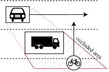
Figure 1: The ego vehicle is travelling with a constant speed and can observe a stopped truck on its right. The area behind the truck is occluded, and is hiding a bicycle that is attempting to cross the road. Both the ego vehicle and the bicycle are unaware of each other, leading to a dangerous situation.

We integrate BiVO into a sampling-based planning algorithm [10] for autonomous driving. The planner samples a set of dynamically feasible trajectories for the ego-vehicle, and selects the most promising trajectory given a hand-crafted cost function. BiVO predictions enter the planner through a collision avoidance term in the cost function. Specifically, we sample a large number of trajectories from BiVO along with their probabilities, and calculate the expected collision cost, treating the predicted occluded agent trajectories the same way as predictions for visible traffic agents.

To validate BiVO, we use real-world trajectory data from the nuScenes Prediction dataset [1], both for direct prediction metrics, open-loop planning metrics, and in a closed-loop replay simulation. As one would expect, occluded objects rarely affect the desired trajectories of our planner, but when they do, reasoning about occlusions significantly improves the plan quality; and BiVO is significantly more effective than alternative learned models that were not designed for planning (see Section VI-B).

In summary, the contributions of this paper are as follows:

• We introduce a generative model, BiVO, based on variational autoencoders that is able to produce trajectories of occluded vehicles.

• We integrate BiVO into a fast sampling-based planning algorithm and evaluate it in open and closed-loop replay simulation with the real-world nuScenes dataset.

• We demonstrate that BiVO predictions integrated into planning leads to better motion plans in critical scenarios.

• To the best of our knowledge we are the first to integrate a learned occlusion model with a planning algorithm for autonomous driving.

II Related Work

Detecting and reasoning with occluded objects in robotics has an extensive literature [2, 6]. In the context of autonomous vehicles, occlusions can be of critical importance. Indeed, prior work has proposed various methods that predict and/or plan with occluded traffic agents.

Planning with occluded agents:  Planning algorithms that reason with occluded agents typically rely on handcrafted occlusion models. For example, [15] propose an approach to predicting the presence of a vehicle coming out of an occluded region and ensures the existence of a fail-safe manoeuvre. [20] extend this work by eliminating some of the occluded traffic by reasoning about the history of occlusions. [21] propose a method of navigating through traffic with occluded regions by making sure a potentially hidden pursuer should never intersect with the set of possible inevitable collision states. [8] use a model-driven approach that infers a joint distribution over the state of the occluded areas and the goals of other vehicles, using the observed trajectories of the vehicles.

In contrast to these hand-crafted approaches, we propose a data-driven approach that learns a model of occluded agents from real-world data.

Data-driven occlusion models:  Learning based models for occluded object prediction include [18, 17, 7]. However these models make assumptions about static objects or environments which are not pertinent in urban driving. Some learned models can handle dynamic traffic agents. Notably, [9] use an autoencoder architecture to infer the surroundings of visible objects and later reconstruct them into occupancy grid maps that encode the probability of occupied areas in 2D space. However, it is not straightforward to integrate approaches that make occupancy predictions of areas with existing planners, since the predictions lack the information on how agents might emerge out of occlusions and interfere with the ego vehicle.

In our work, we predict dynamic agents together with their possible future trajectories instead of only occluded areas. Our model’s predictions are key to integration with existing downstream planners that make use of probabilistic predictions of future trajectories.

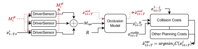
Figure 2: The information flow for BiVO. The elements in red are only provided during training. During execution, the DriverSensor(s) reconstruct the surroundings of visible vehicles using only their observed trajectories. The OGMs are combined and given to a generative model which predicts plausible trajectories of occluded vehicles. The planner can then use that information to decide on a trajectory for the ego vehicle.

III Technical Preliminaries

Variational Autoencoders: Variational autoencoders [11] (VAEs) are generative models that aim to learn a density function over some unobserved latent variables $Z$ given a dataset input $x\in X$. Given an unknown true posterior $p(z|x)$, VAEs approximate it with a parametric distribution $q_{\theta}(z|x)$. The KL-divergence from the parametric distribution to the true posterior can be computed using:

$$\operatorname*{D_{KL}}(q_{\theta}(z|x)\|p(z|x))=\log p(x)\\ -\mathbb{E}_{z\sim q_{\theta}(z|x)}[\log p_{u}(x|z)]+\operatorname*{D_{KL}}(q_{\theta}(z|x)\|q(z)),$$

where $\operatorname*{D_{KL}}$ is the KL divergence between two distributions, and the log-evidence term $\log p(x)$ is constant. The expectation and the KL-divergence (second line) are commonly called the negative evidence lower bound (ELBO). Minimising the ELBO is equivalent to minimising the KL-divergence between the parametric and the true posterior.

States and trajectories: A state $s^{i}_{t}$ for a vehicle $i$ is defined as the location, heading, velocity, and acceleration at the current timestep $t$. A trajectory $x^{i}_{t:t+T}$ is a sequence of states $s^{i}_{t},s^{i}_{t+1},\dots,s^{i}_{t+T}$ that defines how an agent $i$ moved in time $T$.

Agents: We will refer to the controlled vehicle as “ego”. Other vehicles that are not controlled by the planner, pedestrians, or other road users will be referred to as “agents”. Agents can be visible by the ego if they are in the line of sight, or occluded if there is an obstacle blocking their view (further details of this calculation is in Section VI-A).

Occupancy grid maps: OGMs encode the occupancy of an area. $M_{i}^{\text{obs}}\in[0,1]^{H,W}$ is the $H\times W$ area surrounding agent $i$ in a $1\times 1$ meter resolution, and each grid cell contains $1$ if it is occupied or $0$ if free. Locations that are not visible with a direct line of sight from the position of vehicle $i$ are marked as occluded with a value $0.5$. $M_{i}^{\text{gt}}$ is the ground truth occupancy map of the same area.

IV Bi-Level Variational Occlusion Models

The objective of our occlusion model is to generate likely trajectories for agents emerging from occluded regions, given a known map of occluded regions, the past and present state of visible agents, and a lane graph.

Our approach, BiVO, is shown in Fig. 2. We break down the problem into two subproblems and train separate CVAE models for each. Intuitively, the first step locates the subspace of occluded areas that have high potential of hidden objects; and the second step infers how these hidden object may emerge from the occluded space. Overall, BiVO parameterizes a distribution over trajectories that start from known occluded regions, and allows fast sampling from this distribution for subsequent planning.

IV-A Reasoning about the Behaviour of Others

The first component of our architecture, the DriverSensor, is based on the work of [9]. The DriverSensor model aims to produce OGMs with probabilities of obstacles existing in the respective grid cells (e.g. Fig. 3). The DriverSensor’s CVAE is trained to reconstruct the OGMs of the immediate surroundings of visible cars by only observing their state (past locations, velocities, and accelerations). These reconstructions are later combined into a single, larger OGM centered on the ego vehicle using the theory of belief functions (or Dempster-Shafer theory) [3]. The reconstruction $M_{\text{ego}}\in[0,1]^{H,W}$ is an $H,W$ grid map that contains the probabilities of each cell being occupied.

We use a similar architecture and loss function to [9] with a key modification as follows. The DriverSensor CVAE with discrete latent space consists of encoders $p(z|x^{i}_{t-T:t})$ and $q(z|x^{i}_{t-T:t},M_{i}^{\text{gt}})$; and decoder $p(M_{i}^{\text{gt}}|z)$. During training we minimise the loss $\mathcal{L}_{DS}$:

$$\mathcal{L}_{\text{DS}}=-\mathbb{E}_{z\sim q(z|x_{t-T:t})}\log p(M_{i}^{\text{gt}}|z)\\ +\beta\operatorname*{D_{KL}}(q(z|x^{i}_{t-T:t},M_{i}^{\text{gt}})\|p(z|x^{i}_{t-T:t}))\\ -\mathcal{I}_{q}(M_{i}^{\text{gt}};z)+(1-\beta)\mathcal{H}(q(\cdot|x^{i}_{t-T:t},M_{i}^{\text{gt}})),$$

where $\mathcal{I}$ is the mutual information and $\beta$ is a hyperparameter annealed from zero to one. We added the entropy term $\mathcal{H}$, calculated over the batch, that maximises the number of active discrete latent classes in the beginning of training. We found this to be important to avoid the collapse of the discrete latent space.

In the rest of the document, we denote by $M_{\text{ego}}$ the most likely reconstruction of the fused DriverSensors. More details on the DriverSensor can be found in the original work [9].

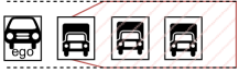
Figure 3: Illustrative example for using people as sensors. The ego vehicle can only observe the truck directly in front of it, which has stopped without any obvious reason. Even if the ego vehicle cannot directly observe the other vehicles (under the red striped area), it can assign a high probability mass on the possibility of an obstacle blocking the truck’s way, just by reasoning about the stopped truck.

IV-B Occluded Trajectory Generation

An occupancy grid map, even the ground truth OGM, cannot be used to extrapolate the movement of hidden vehicles into the future. Our goal is to generate probable future trajectories of vehicles emerging from an occluded area. These trajectories can then be used as a component in a planning system. To model vehicles emerging from the occluded areas, we use the generative properties of a variational autoencoder. By doing so, we aim to learn from real-world data a distribution of vehicle trajectories that emerge from occluded areas.

The occlusion model consists of a CVAE that receives an occluded trajectory $x^{\text{occl}}_{t:T}$ as an input to the encoder. An “occluded trajectory” is defined as a trajectory that originates in an occluded area of the ego OGM (i.e. $M^{\text{obs}}_{\text{ego}}=0.5$ at the location of the agent $i$ at time $t$). The decoder is further conditioned on the latent variable $z$, a raster of the road layout $R$, and finally the most-likely reconstruction of the nearby occupancy grid map $M_{\text{ego}}$.

Formally, the occluded trajectories are projected into a latent space through the posteriors $q(z|x^{\text{occl}}_{t:T})$ and $p(z|x^{\text{occl}}_{t:T},R,M_{\text{ego}})$. To learn the distribution, we optimise the objective $D_{KL}(q(z|x^{\text{occl}}_{t:T})||p(z|x^{\text{occl}}_{t:T},R,M_{\text{ego}})$, where $D_{KL}$ is the KL divergence between two distributions. The evidence lower bound (ELBO) becomes:

$$\mathcal{L}_{\text{Gen}}=-\mathbb{E}_{z\sim q(z|x^{\text{occl}}_{t:t+T})}\log p(x^{\text{occl}}_{t:t+T}|R,M_{\text{ego}})\\ +D_{KL}(q(z|x^{\text{occl}}_{t:t+T},R,M_{\text{ego}})||p(z|R,M_{\text{ego}}))$$ (1)

Therefore, the occluded areas in the field of vision of the ego vehicle hide a distribution from which we can sample trajectories. After training the generative model on real-world data, we sample $z\sim N(0,1)$ which can then be decoded as trajectories using the VAE’s decoder.

V Planning with BiVO

The generated trajectories can be directly integrated into a planning component. Our planner follows a common approach for AV planning, where we first generate a set of candidate trajectories, and then choose the most promising trajectory based on a hand-crafted cost function.

More specifically, we use the planning algorithm of [10]. The algorithm generates $J$ dynamically feasible candidate trajectories $x^{1\dots j}_{t:T}$, by first sampling terminal points based on the lane map, connecting the current state to the terminal point through spline interpolation, and filtering the trajectories that violate control limits. We then evaluate each of these trajectories using handcrafted cost components, specifically

$$C=C_{\text{hd}}+C_{\text{vd}}+C_{\text{ef}}+C_{\text{col}}+C_{\text{goal}},$$ (2)

where $C_{\text{vd}}$ and $C_{\text{hd}}$ are the lane and heading deviation respectively, calculated from the nearest lane at each spline point. $C_{\text{ef}}$ is the effort cost, calculated as the acceleration squared and $C_{\text{goal}}$ is the distance from the goal. In experiments we simply define the goal as the ground truth future state at time $t+T$.

Finally, $C_{\text{col}}$ is the collision cost, calculated using the trajectories with the visible but also with the predicted vehicles. We define this collision cost using:

$$C_{\text{col}}=\sum_{i=1}^{N}{\sum_{\tau=t}^{T}{\phi(s^{i}_{\tau}-s^{\text{ego}}_{\tau})}}+\sum_{k=1}^{K}{\pi_{k}\sum_{\tau=t}^{T}{\phi(s^{k}_{\tau}-s^{\text{ego}}_{\tau})}},$$

where $i$ iterates over the $N$ visible agents (we use ground truth future trajectories for simplicity), $k$ iterates over the $K$ trajectories sampled by our method, and $\phi$ is a radial basis function. $\pi_{k}$ represents the probability of trajectory $k$ and is defined as $\frac{1}{K}\pi_{e}$ with $\pi_{e}$ being the prior for the existence of any occluded agent.

Eventually, to find the desired ego trajectory, the planner calculates:

$$\hat{x}^{\text{ego}}_{t:t+T}=\operatorname*{arg\,min}_{j}C(x^{j}_{t:t+T})$$ (3)

VI Experiments

We evaluate BiVO using the nuScenes dataset [1]. We aim to evaluate i) the quality of generated trajectories, and ii) how planning is affected when using these trajectories.

VI-A Data Processing & Experimental Details

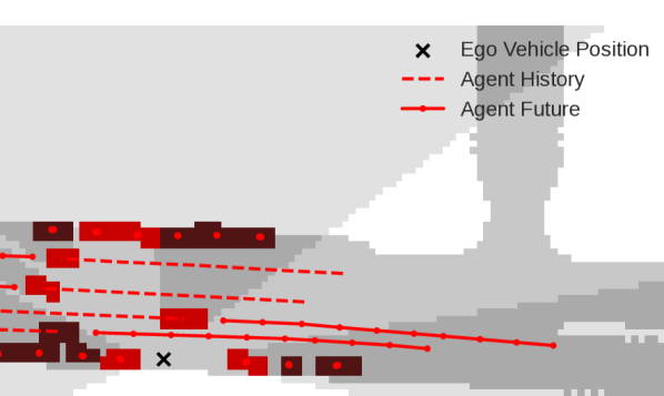
Figure 4: Line of sight calculation starting from the ego vehicle position. Agents that are in a direct line of sight (calculated from the X location with a 1x1m resolution) can be observed by the ego agent (bright red). Areas that are not in a line of sight are denoted by a grey shadow, including the dark red agents.

The original nuScenes dataset [1] does not contain occlusion information, therefore we calculate at every timestep the occlusion using a direct line-of-sight method. Specifically, we first create a raster of the surrounding scene that includes the neighbour agents in a $1\times 1$ meter grid. We draw lines starting at the centre of the ego vehicle towards the edges of the map, which however stop when an agent is encountered. Any area covered by those lines is considered visible, otherwise it is considered occluded (see Fig. 4). During planning, we only use the trajectories of visible vehicles (except in the NuScenes Oracle baseline).

	Training $\downarrow$	Test $\downarrow$
BiVO	$38.82\pm 0.42$	$48.68\pm 0.61$
Trajectory CVAE	$45.98\pm 0.13$	$52.71\pm 0.10$
Simple CVAE	$68.32\pm 0.06$	$73.52\pm 0.06$

TABLE I: ELBO at the end of training for both training and test sets. Mean and standard error over three training seeds.

To train our models, we first independently train the DriverSensor model on the nuScenes data to produce the $M_{i}$ OGMs which are then merged into $M_{\text{ego}}$. After the DriverSensor model is trained, its output is used to train our VAE model by minimising the ELBO loss (Eq. 1).

For DriverSensor, we used the hyperparameters specified in [9]. For our occlusion model, we set the learning rate to $3e-4$, and we used four linear layers for encoding and decoding the trajectories. We used the VQ-VAE [14] for our autoencoder architecture. We trained for a total of five epochs on the nuScenes dataset, on timesteps that have at least $T$ seconds of history and future. Finally we used $T=5s$ as a time horizon for both planning and trajectory reconstruction. Any generated trajectories that are not feasible or begin on a non-occluded area are filtered out.

	Open loop $\downarrow$ (all scenes)	Open loop $\downarrow$ (critical scenes)	Closed loop $\downarrow$ (all scenes)
NuScenes Oracle	4.4922	5.7410	0.3502
BiVO (ours)	4.8932 (+8.92%)	6.0843 (+5.97%)	0.3472 (-0.85%)
Trajectory CVAE	5.2639 (+17.17%)	6.2254 (+8.43%)	0.3479 (-0.65%)
DriverSensor [9]	5.1949 (+15.64%)	6.3268 (+10.20%)	0.3532 (+0.85%)
Occlusion agnostic baseline	4.5062 (+0.31%)	6.2021 (+8.03%)	0.3503 (+0.02%)

TABLE II: Average hindsight cost for our method and various baselines in the nuScenes dataset (lower is better). In parenthesis we denote the percentage increase of cost over the NuScenes Oracle.

VI-B Baselines

We compare BiVO with the baselines described below.

Occlusion Agnostic: This baseline assumes that occluded spaces do not contain any occluded agents and should not affect the trajectory of the ego vehicle. This is equivalent to setting assigning a zero probability to any generated trajectories ($\pi_{k}=0$).

Trajectory CVAE: Uses a CVAE in a similar configuration to our method. However, it does not make use of a reconstructed OGM $M_{\text{ego}}$ which acts as a prior to the trajectory generation process. To keep the number of parameters and architecture configuration fair, we instead use the an OGM that notates the locations that are occluded (i.e. $M^{\text{obs}}_{\text{ego}}$, see Section IV-A).

DriverSensor: The SOTA occlusion model of [9] that outputs an OGM instead of trajectories. To integrate the model with planning, we generate agents in a heuristic manner, selecting the highest-valued location(s) in $M_{\text{ego}}$ and generating occluded vehicles there. While this method could potentially be better at locating the initial location of occluded agents, it does not learn how these agents behave or affect the ego vehicle.

NuScenes Oracle: The trajectories of occluded vehicles are fully observed and used by the calculations of this baseline. The collision cost of Eq. 2 uses all nearby agents for evaluating Eq. 3. Notably, this baseline is prone to errors in the dataset, and while we do not explicitly remove vehicles not in the line of sight, the dataset itself could contain such occlusions (from trucks, walls, objects, or even sensor failures). However, in the open-loop evaluation this baseline acts as a lower bound to the minimised cost since it uses the same data for calculation of the hindsight cost.

VI-C Experimental Results

(a) An agent driving straight
in an occluded space.

(b) An oncoming traffic agent
in the opposing side of the road.

(c) A pedestrian appearing
behind parked vehicles.

(d) A generated trajectory next to an actual occluded agent.

Figure 5: Examples of trajectories (in blue) generated by BiVO. Darker areas are occluded, bright red cars are visible.

Our final qualitative results are reported in Tables I and II and our qualitative results are in Figs. 6 and 5. In this section, we provide a further analysis of these results.

Table I shows the ELBO loss as a proxy to the marginal likelihood of $x^{\text{occl}}_{t:t+T}$ under the model. BiVO achieves a lower ELBO for both the training and the test set. We also compared with a simple CVAE model that does not use either $M_{\text{ego}}$ or $M^{\text{obs}}_{\text{ego}}$. These results show that information about the occluded areas is important, and further that our bi-level approach can make use of the information inferred by the DriverSensors.

Our planning experiments show that occluded agents do not often interfere with the ego trajectory. Specifically, in $98\%$ of the scenes in the nuScenes test set, the NuScenes Oracle and the Occlusion Agnostic baselines select identical trajectories. This is not surprising, as many of the scenes contain relatively simple and safe scenarios, such as driving on a straight path. Indeed, much of the driving that happens in a normal situation does not deal with stray agents as motivated in Fig. 1, but instead any agents come in the field of view of the ego vehicle long before any preventive action needs to be taken. That said, our algorithms must consider such situations even if they are rare in nature.

Table II shows the mean hindsight cost of the selected trajectories when planning with different occlusion models. We report the hindsight cost using the ground truth occluded vehicles, i.e. $\hat{x}^{\text{ego}}_{t:t+T}$ using Eq. 3 is first calculated, then the same cost function is reevaluated but now using the ground truth trajectories. So, the hindsight cost is the cost of the selected trajectory evaluated under the fully observable current and future states (i.e. the cost function of NuScenes Oracle). The open-loop results are split into two sets: the first set contains the full nuScenes evaluation dataset; the second set contains the “Critical Scenes” defined as any scenes where there is at least one timestep where the cost of the best trajectory selected by the Occlusion Agnostic and NuScenes Oracle baselines are different.

Open loop (all scenes): In the full validation dataset, the Occlusion Agnostic baseline performs very closely to the fully observable (NuScenes Oracle) lower bound. This is largely a result of the simpler scenes that do not contain any important occluded agents. BiVO selects trajectories with lower hindsight cost ($+8.92\%$ increase over the NuScenes Oracle) than both Trajectory CVAE ($+17.17\%$) and the DriverSensor ($+15.64\%$).

Open Loop (critical scenes): In the critical scenes, where occlusions do make a difference in the decision making process, our method has lower hindsight cost than all baselines, including Occlusion Agnostic. Specifically, BiVO only has a $+5.97\%$ increase over the NuScenes Oracle with Trajectory CVAE and DriverSensor having $+8.43\%$ and $+10.20\%$ respectively. The increased hindsight cost of Occlusion Agnostic ($+8.03\%$) indicates an increased collision cost over BiVO. Therefore, in the critical scenes, our experiments show that our method selects trajectories that consider the existence of occluded agents that might interfere with the ego vehicle and makes better trajectory decisions.

Closed loop (all scenes): In the closed-loop evaluation (right-most column in Table II) we present the hindsight cost of the actual trajectory. BiVO selects trajectories with the lowest hindsight cost ($-0.85\%$). This suggests that BiVO trajectories are even better than the NuScenes Oracle, which is also the case for Trajectory CVAE ($-0.65\%$). One possible reason is that scenes in the nuScenes dataset may contain occlusions themselves. Occluded agents may be missing from the data, and in some situations such agents may appear suddenly interfering with the ego vehicle. Further, in our experiments non-ego agents follow their recorder “ground truth” trajectory, therefore they do not react to the ego’s trajectory which may cause unreasonable collisions. To mitigate this issue we reduced the maximum time per scene to 15 seconds. DriverSensor ($+0.85\%$) and Occlusion Agnostic ($+0.02\%$) still select trajectories with higher hindsight cost.

In conclusion, our experiments show that BiVO comes with the trade-off of slightly costlier trajectories ($+8.58\%$ over being agnostic reasoning about occlusions) in regular driving scenarios but offers an improvement ($-1.93\%$) in critical situations. As we show in Section VI-D and Fig. 6, the selected trajectories are reasonable and lead to preferred states when occluded agents ultimately become visible.

In addition, BiVO can be used in real-time. In our experiments, inference only requires a few milliseconds, significantly less that the planner’s frequency, depending on the quantity of visible neighbouring agents and the number of samples drawn from the generative model (we used 1000).

VI-D Qualitative Results

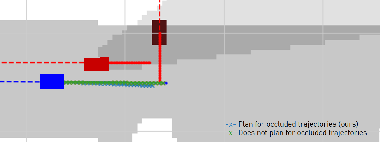
Figure 6: Reconstruction of example in Fig. 1. The ego vehicle (blue) cannot observe the occluded agent crossing the road. The (bright red) agent that is visible, has noticed the occluded agent and is breaking. We plot the trajectory selected by Occlusion Agnostic and our method. Notably, even if our method cannot observe the occluded agent, it chooses a trajectory slightly to the right and with lower speed.

Trajectories sampled from BiVO: In Fig. 5, we present examples of trajectories drawn from BiVO. The trajectories were generated by sampling $z\sim N(0,1)$ once and combining them with the raster $R$ and the reconstruction $M^{\text{ego}}$. While in those figures we draw a single sample for clarity, during the planning experiments we sample up to 1000 trajectories per scene.

Many of the trajectories drawn from BiVO are plausible for the respective occluded areas and road layouts. For instance, both Figs. 5(b) and 5(c) show agents driving normally in their assigned lanes. This shows a benefit of our approach to learn from data: trajectories are often close to what would be encountered in the real world. Figure 5(d) even generates a trajectory very close to a vehicle that indeed exists, but is hidden from the model and the planner. Finally, Fig. 5(c) shows a more aggressive trajectory, a pedestrian who is emerging from two parked vehicles, a very dangerous situation in the real world, and one that must be accounted for (also see Fig. 6). It has to be noted that individual generated trajectories do not have a significant weight in the planner’s calculation. Instead, the planner sums over hundreds of such trajectories to grasp the underlying distribution of plausible occluded agents.

Planning in a dangerous situation: To build an intuition of the selected trajectories of BiVO, we have reconstructed the motivational example of Fig. 1 in Fig. 6. The ego vehicle is depicted in blue, and is moving without being able to observe the occluded agent (dark red). The only information of the existence of any obstacle in the ego’s path, would be the visible agent slowing down. However, even that might not be enough to provide evidence of any obstacle. Our method still decides on a trajectory that is slightly slower, but also slightly away from the occluded area. While this is a worst-case scenario, a vehicle that uses BiVO and considers the learned distribution of occluded vehicles will i) have slower speed ($3.65m/s$ vs $4m/s$) , ii) be further away (by $1.6m$), and iii) observe the occluded agent sooner than not reasoning about occlusions in its planning.

VII Conclusion & Future Work

We introduced BiVO, a bi-level variational autoencoder model to generate plausible agent trajectories in occluded areas. We trained this model in the real-world nuScenes dataset and integrated it with a simple sampling-based planner. The planner produces trajectories that take into consideration occlusions and while they have a possibly higher hindsight cost in simple driving scenarios, they do offer positional advantages in critical scenarios where occluded agents are indeed important to driving. In the future, we aim to improve our model by including realistic vehicle dynamics, and integrating previously observed information on occluded objects.

References

- [1] Holger Caesar, Varun Bankiti, Alex H. Lang, Sourabh Vora, Venice Erin Liong, Qiang Xu, Anush Krishnan, Yu Pan, Giancarlo Baldan and Oscar Beijbom “nuScenes: A multimodal dataset for autonomous driving” In CVPR, 2020
- [2] Himanshu Chandel and Sonia Vatta “Occlusion detection and handling: a review” In International Journal of Computer Applications 120.10 Citeseer, 2015
- [3] A.. Dempster “Upper and Lower Probabilities Induced by a Multivalued Mapping” In The Annals of Mathematical Statistics 38.2 Institute of Mathematical Statistics, 1967, pp. 325–339 DOI: 10.1214/aoms/1177698950
- [4] Julie Dequaire, Peter Ondruska, Dushyant Rao, Dominic Zeng Wang and Ingmar Posner “Deep tracking in the wild: End-to-end tracking using recurrent neural networks” In Int. J. Robotics Res. 37.4-5, 2018, pp. 492–512
- [5] Alberto Elfes “Using occupancy grids for mobile robot perception and navigation” In Computer 22.6 IEEE, 1989, pp. 46–57
- [6] Shane Gilroy, Edward Jones and Martin Glavin “Overcoming occlusion in the automotive environment—A review” In IEEE Transactions on Intelligent Transportation Systems 22.1 IEEE, 2019, pp. 23–35
- [7] Yutao Han, Jacopo Banfi and Mark Campbell “Planning Paths Through Unknown Space by Imagining What Lies Therein” In 4th Conference on Robot Learning, CoRL 2020, 16-18 November 2020, Virtual Event / Cambridge, MA, USA 155, Proceedings of Machine Learning Research PMLR, 2020, pp. 905–914
- [8] Josiah P. Hanna, Arrasy Rahman, Elliot Fosong, Francisco Eiras, Mihai Dobre, John Redford, Subramanian Ramamoorthy and Stefano V. Albrecht “Interpretable Goal Recognition in the Presence of Occluded Factors for Autonomous Vehicles” In IEEE/RSJ International Conference on Intelligent Robots and Systems (IROS), 2021
- [9] Masha Itkina, Ye-Ji Mun, Katherine Driggs-Campbell and Mykel J. Kochenderfer “Multi-Agent Variational Occlusion Inference Using People as Sensors” In 2022 International Conference on Robotics and Automation (ICRA), 2022, pp. 4585–4591 DOI: 10.1109/ICRA46639.2022.9811774
- [10] Peter Karkus, Boris Ivanovic, Shie Mannor and Marco Pavone “DiffStack: A Differentiable and Modular Control Stack for Autonomous Vehicles” In 6th Annual Conference on Robot Learning, 2022 URL: https://openreview.net/forum?id=teEnA3L4aRe
- [11] Diederik P. Kingma and Max Welling “Auto-Encoding Variational Bayes” In International Conference on Learning Representations, 2014 URL: http://arxiv.org/abs/1312.6114
- [12] Yannik Nager, Andrea Censi and Emilio Frazzoli “What lies in the shadows? Safe and computation-aware motion planning for autonomous vehicles using intent-aware dynamic shadow regions” In International Conference on Robotics and Automation, ICRA 2019, Montreal, QC, Canada, May 20-24, 2019 IEEE, 2019, pp. 5800–5806 DOI: 10.1109/ICRA.2019.8793557
- [13] Simon Timothy O’Callaghan and Fabio T. Ramos “Gaussian process occupancy maps” In Int. J. Robotics Res. 31.1, 2012, pp. 42–62
- [14] Aäron Oord, Oriol Vinyals and Koray Kavukcuoglu “Neural Discrete Representation Learning” In Advances in Neural Information Processing Systems 30: Annual Conference on Neural Information Processing Systems 2017, December 4-9, 2017, Long Beach, CA, USA, 2017, pp. 6306–6315 URL: https://proceedings.neurips.cc/paper/2017/hash/7a98af17e63a0ac09ce2e96d03992fbc-Abstract.html
- [15] Piotr Franciszek Orzechowski, Annika Meyer and Martin Lauer “Tackling Occlusions & Limited Sensor Range with Set-based Safety Verification” In 21st International Conference on Intelligent Transportation Systems, ITSC 2018, Maui, HI, USA, November 4-7, 2018 IEEE, 2018, pp. 1729–1736
- [16] Jae Sung Park and Dinesh Manocha “HMPO: Human Motion Prediction in Occluded Environments for Safe Motion Planning” In Robotics: Science and Systems XVI, Virtual Event / Corvalis, Oregon, USA, July 12-16, 2020, 2020 DOI: 10.15607/RSS.2020.XVI.051
- [17] Pulak Purkait, Christopher Zach and Ian D. Reid “Seeing Behind Things: Extending Semantic Segmentation to Occluded Regions” In 2019 IEEE/RSJ International Conference on Intelligent Robots and Systems, IROS 2019, Macau, SAR, China, November 3-8, 2019 IEEE, 2019, pp. 1998–2005
- [18] Samuel Schulter, Menghua Zhai, Nathan Jacobs and Manmohan Chandraker “Learning to Look around Objects for Top-View Representations of Outdoor Scenes” In Computer Vision - ECCV 2018 - 15th European Conference, Munich, Germany, September 8-14, 2018, Proceedings, Part XV 11219, Lecture Notes in Computer Science Springer, 2018, pp. 815–831
- [19] Kihyuk Sohn, Honglak Lee and Xinchen Yan “Learning Structured Output Representation using Deep Conditional Generative Models” In Advances in Neural Information Processing Systems 28 Curran Associates, Inc., 2015 URL: https://proceedings.neurips.cc/paper/2015/file/8d55a249e6baa5c06772297520da2051-Paper.pdf
- [20] Lingguang Wang, Christoph Burger and Christoph Stiller “Reasoning about Potential Hidden Traffic Participants by Tracking Occluded Areas” In 24th IEEE International Intelligent Transportation Systems Conference, ITSC 2021, Indianapolis, IN, USA, September 19-22, 2021 IEEE, 2021, pp. 157–163
- [21] Zixu Zhang and Jaime F. Fisac “Safe Occlusion-Aware Autonomous Driving via Game-Theoretic Active Perception” In Robotics: Science and Systems XVII, Virtual Event, July 12-16, 2021, 2021