Strategies for single-shot discrimination of process matrices

Abstract.

The topic of causality has recently gained traction quantum information research. This work examines the problem of single-shot discrimination between process matrices which are an universal method defining a causal structure. We provide an exact expression for the optimal probability of correct distinction. In addition, we present an alternative way to achieve this expression by using the convex cone structure theory. We also express the discrimination task as semidefinite programming. Due to that, we have created the SDP calculating the distance between process matrices and we quantify it in terms of the trace norm. As a valuable by-product, the program finds an optimal realization of the discrimination task. We also find two classes of process matrices which can be distinguished perfectly. Our main result, however, is a consideration of the discrimination task for process matrices corresponding to quantum combs. We study which strategy, adaptive or non-signalling, should be used during the discrimination task. We proved that no matter which strategy you choose, the probability of distinguishing two process matrices being a quantum comb is the same.

1. Introduction

The topic of causality has remained a staple in quantum physics and quantum information theory for recent years. The idea of a causal influence in quantum physics is best illustrated by considering two characters, Alice and Bob, preparing experiments in two separate laboratories. Each of them receives a physical system and performs an operation on it. After that, they send their respective system out of the laboratory. In a causally ordered framework, there are three possibilities: Bob cannot signal to Alice, which means the choice of Bob’s action cannot influence the statistics Alice records (denoted by $A\prec B$), Alice cannot signal to Bob ($B\prec A$), or neither party can influence the other $(A||B)$. A causally neutral formulation of quantum theory is described in terms of quantum combs [1].

One may wonder if Alice’s and Bob’s action can influence each other. It might seem impossible, except in a world with closed time-like curves (CTCs) [2]. But the existence of CTCs implies some logical paradoxes, such as the grandfather paradox [3]. Possible solutions have been proposed in which quantum mechanics and CTCs can exist and such paradoxes are avoided, but modifying quantum theory into a nonlinear one [4]. A natural question arises: is it possible to keep the framework of linear quantum theory and still go beyond definite causal structures?

One such framework was proposed by Oreshkov, Costa and Brukner  [5]. They introduced a new resource called a process matrix – a generalization of the notion of quantum state. This new approach has provided a consistent representation of correlations in casually and non-causally related experiments. Most interestingly, they have described a situation that two actions are neither causally ordered and one cannot say which action influences the second one. Thanks to that, the term of causally non-separable (CNS) structures started to correspond to superpositions of situations in which, roughly speaking, Alice can signal to Bob, and Bob can signal to Alice, jointly. A general overview of causal connection theory is described in [6].

The indefinite causal structures could make a new aspect of quantum information processing. This more general model of computation can outperform causal quantum computers in specific tasks, such as learning or discriminating between two quantum channels [7, 8, 9]. The problem of discriminating quantum operations is of the utmost importance in modern quantum information science. Imagine we have an unknown operation hidden in a black box. We only have information that it is one of two operations. The goal is to determine an optimal strategy for this process that achieves the highest possible probability of discrimination. For the case of a single-shot discrimination scenario, researchers have used different approaches, with the possibility of using entanglement in order to perform an optimal protocol. In [10], Authors have shown that in the task of discrimination of unitary channels, the entanglement is not necessary, whereas for quantum measurements [11, 12, 13], we need to use entanglement. Considering multiple-shot discrimination scenarios, researchers have utilized parallel or adaptive approaches. In the parallel case, we establish that the discrimination between operations does not require pre-processing and post-processing. One example of such an approach is distinguishing unitary channels [10], or von Neumann measurements [14]. The case when the black box can be used multiple times in an adaptive way was investigated by the authors of [15, 16], who have proven that the use of adaptive strategy and a general notion of quantum combs can improve discrimination.

In this work, we study the problem of discriminating process matrices in a single-shot scenario. We obtain that the probability of correct distinction process matrices is strictly related to the Holevo-Helstrom theorem for quantum channels. Additionally, we write this result as a semidefinite program (SDP) which is numerically efficient. The SDP program allows us to find an optimal discrimination strategy. We compare the effectiveness of the obtained strategy with the previously mentioned strategies. The problem gets more complex in the case when we consider the non-causally ordered framework. In this case, we consider the discrimination task between two process matrices having different causal orders.

This paper is organized as follows. In Section 2 we introduce necessary mathematical framework. Section 3 is dedicated to the concept of process matrices. Section 4 presents the discrimination task between pairs of process matrices and calculate the exact probability of distinguishing them. Some examples of discrimination between different classes of process matrices are presented in Section 5. In Section 5.1, we consider the discrimination task between free process matrices, whereas in Section 5.2 we consider the discrimination task between process matrices being quantum combs. In Section 5.3, we show a particular class of process matrices having opposite causal structures which can be distinguished perfectly. Finally, Section 6 and Section 7 are devoted to semidefinite programming, thanks to which, among other things, we obtain an optimal discrimination strategy. In Section 8, we analyze an alternative way to achieve this expression using the convex cone structure theory. Concluding remarks are presented in the final Section 9. In the Appendix A, we provide technical details about the convex cone structure.

2. Mathematical preliminaries

Let us introduce the following notation. Consider two complex Euclidean spaces and denote them by $\mathcal{X},\mathcal{Y}$. By $\mathrm{L}(\mathcal{X},\mathcal{Y})$ we denote the collection of all linear mappings of the form $A:\mathcal{X}\rightarrow\mathcal{Y}$. As a shorthand put $\mathrm{L}(\mathcal{X})\coloneqq\mathrm{L}(\mathcal{X},\mathcal{X}).$ By $\mathrm{Herm}(\mathcal{X})$ we denote the set of Hermitian operators while the subset of $\mathrm{Herm}(\mathcal{X})$ consisting of positive semidefinite operators will be denoted by $\mathrm{Pos}(\mathcal{X})$. The set of quantum states, that is positive semidefinite operators $\rho$ such that $\operatorname{tr}\rho=1$, will be denoted by $\Omega(\mathcal{X})$. An operator $U\in\mathrm{L}\left(\mathcal{X}\right)$ is unitary if it satisfies the equation $UU^{\dagger}=U^{\dagger}U={\rm 1l}_{\mathcal{X}}$. The notation $\mathrm{U}\left(\mathcal{X}\right)$ will be used to denote the set of all unitary operators. We will also need a linear mapping of the form $\Phi:\mathrm{L}(\mathcal{X})\rightarrow\mathrm{L}(\mathcal{Y})$ transforming $\text{L}(\mathcal{X})$ into $\text{L}(\mathcal{Y})$. The set of all linear mappings is denoted $\mathrm{M}(\mathcal{X},\mathcal{Y})$. There exists a bijection between set $\mathrm{M}(\mathcal{X},\mathcal{Y})$ and the set of operators $\mathrm{L}(\mathcal{Y}\otimes\mathcal{X})$ known as the Choi [17] and Jamiołkowski [18] isomorphism. For a given linear mapping $\Phi_{M}:\mathrm{L}(\mathcal{X})\rightarrow\mathrm{L}(\mathcal{Y})$ corresponding Choi matrix $M\in\mathrm{L}(\mathcal{Y}\otimes\mathcal{X})$ can be explicitly written as

$$M\coloneqq\sum_{i,j=0}^{\dim(\mathcal{X})-1}\Phi_{M}(|i\rangle\!\langle j|)\otimes|i\rangle\!\langle j|.$$ (1)

We will denote linear mappings by $\Phi_{M},\Phi_{N},\Phi_{R}$ etc., whereas the corresponding Choi matrices as plain symbols: $M,N,R$ etc. Let us consider a composition of mappings $\Phi_{R}=\Phi_{N}\circ\Phi_{M}$ where $\Phi_{N}:\mathrm{L}(\mathcal{Z})\rightarrow\mathrm{L}(\mathcal{Y})$ and $\Phi_{M}:\mathrm{L}(\mathcal{X})\rightarrow\mathrm{L}(\mathcal{Z})$ with Choi matrices $N\in\mathrm{L}(\mathcal{Z}\otimes\mathcal{Y})$ and $M\in\mathrm{L}(\mathcal{X}\otimes\mathcal{Z})$, respectively. Then, the Choi matrix of $\Phi_{R}$ is given by [19]

$$R=\operatorname{tr}_{\mathcal{Z}}\left[\left({\rm 1l}_{\mathcal{Y}}\otimes M^{T_{\mathcal{Z}}}\right)\left(N\otimes{\rm 1l}_{\mathcal{X}}\right)\right],$$ (2)

where $M^{T_{\mathcal{Z}}}$ denotes the partial transposition of $M$ on the subspace $\mathcal{Z}$. The above result can be expressed by introducing the notation of the link product of the operators $N$ and $M$ as

$$N*M\coloneqq\operatorname{tr}_{\mathcal{Z}}\left[\left({\rm 1l}_{\mathcal{Y}}\otimes M^{T_{\mathcal{Z}}}\right)\left(N\otimes{\rm 1l}_{\mathcal{X}}\right)\right].$$ (3)

Finally, we introduce a special subset of all mappings $\Phi$, called quantum channels, which are completely positive and trace preserving (CPTP). In other words, the first condition reads

$$(\Phi\otimes\mathcal{I_{\mathcal{Z}}})(X)\in\mathrm{Pos}(\mathcal{Y}\otimes\mathcal{Z})$$ (4)

for all $X\in\mathrm{Pos}(\mathcal{X}\otimes\mathcal{Z})$ and $\mathcal{I_{\mathcal{Z}}}$ is an identity channel acts on $\mathrm{L}(\mathcal{Z})$ for any $\mathcal{Z}$, while the second condition reads

$$\operatorname{tr}(\Phi(X))=\operatorname{tr}(X)$$ (5)

for all $X\in\mathrm{L}(\mathcal{X})$.

In this work we will consider a special class of quantum channels called non-signaling channels (or causal channels)  [20, 21]. We say that $\Phi_{N}:\mathrm{L}(\mathcal{X}_{I}\otimes\mathcal{Y}_{I})\rightarrow\mathrm{L}(\mathcal{X}_{O}\otimes\mathcal{Y}_{O})$ is a non-signaling channel if its Choi operator satisfies the following conditions

$$\begin{split}&\operatorname{tr}_{\mathcal{X}_{O}}(N)=\frac{{\rm 1l}_{\mathcal{X}_{I}}}{\dim(\mathcal{X}_{I})}\otimes\operatorname{tr}_{\mathcal{X}_{O}\mathcal{X}_{1}}(N),\\ &\operatorname{tr}_{\mathcal{Y}_{O}}(N)=\frac{{\rm 1l}_{\mathcal{Y}_{I}}}{\dim(\mathcal{Y}_{I})}\otimes\operatorname{tr}_{\mathcal{Y}_{O}\mathcal{Y}_{1}}(N).\end{split}$$ (6)

It can be shown [22] that each non-signaling channel is an affine combination of product channels. More precisely, any non-signaling channel $\Phi_{N}:\mathrm{L}(\mathcal{X}_{I}\otimes\mathcal{Y}_{I})\rightarrow\mathrm{L}(\mathcal{X}_{O}\otimes\mathcal{Y}_{O})$ can be written as

$$\Phi_{N}=\sum_{i}\lambda_{i}\Phi_{S_{i}}\otimes\Phi_{T_{i}},$$ (7)

where $\Phi_{S_{i}}:\mathrm{L}(\mathcal{X}_{I})\rightarrow\mathrm{L}(\mathcal{X}_{O})$ and $\Phi_{T_{i}}:\mathrm{L}(\mathcal{Y}_{I})\rightarrow\mathrm{L}(\mathcal{Y}_{O})$ are quantum channels, $\lambda_{i}\in\mathbb{R}$ such that $\sum_{i}\lambda_{i}=1$. For the rest of this paper, by $\mathbf{NS}(\mathcal{X}_{I}\otimes\mathcal{X}_{O}\otimes\mathcal{Y}_{I}\otimes\mathcal{Y}_{O})$ we will denote the set of Choi matrices of non-signaling channels.

The most general quantum operations are represented by quantum instruments [23, 24], that is, collections of completely positive (CP) maps $\left\{\Phi_{M_{i}}\right\}_{i}$ associated to all measurement outcomes, characterized by the property that $\sum_{i}\Phi_{M_{i}}$ is a quantum channel.

We will also consider the concept of quantum network and tester [25]. We say that $\Phi_{R^{(N)}}$ is a deterministic quantum network (or quantum comb) if it is a concatenation of $N$ quantum channels and $R^{(N)}\in\mathrm{L}\left(\bigotimes_{i=0}^{2N-1}\mathcal{X}_{i}\right)$ fulfills the following conditions

$$\begin{split}R^{(N)}&\geq 0,\\ \operatorname{tr}_{\mathcal{X}_{2k-1}}\left(R^{(k)}\right)&={\rm 1l}_{\mathcal{X}_{2k-2}}\otimes R^{(k-1)},\end{split}$$ (8)

where $R^{(k-1)}\in\mathrm{L}\left(\bigotimes_{i=0}^{2k-3}\mathcal{X}_{i}\right)$ is the Choi matrix of the reduced quantum comb with concatenation of $k-1$ quantum channels, $k=2,\ldots,N$. We remind that a probabilistic quantum network $\Phi_{S^{(N)}}$ is equivalent to a concatenation of $N$ completely positive trace non increasing linear maps. Then, the Choi operator $S^{(N)}$ of $\Phi_{S^{(N)}}$ satisfies $0\leq S^{(N)}\leq R^{(N)}$, where $R^{(N)}$ is Choi matrix of a quantum comb. Finally, we recall the definition of a quantum tester. A quantum tester is a collection of probabilistic quantum networks $\left\{R_{i}^{(N)}\right\}_{i}$ whose sum is a quantum comb, that is $\sum_{i}R^{(N)}_{i}=R^{(N)}$, and additionally $\dim(\mathcal{X}_{0})=\dim(\mathcal{X}_{2N-1})=1$.

We will also use the Moore–Penrose pseudo–inverse by abusing notation $X^{-1}\in\mathrm{L}(\mathcal{Y},\mathcal{X})$ for an operator $X\in\mathrm{L}(\mathcal{X},\mathcal{Y})$. Moreover, we introduce the vectorization operation of $X$ defined by $|X\rangle\rangle=\sum_{i=0}^{\dim(\mathcal{X})-1}(X|i\rangle)\otimes|i\rangle$.

3. Process matrices

This section introduces the formal definition of the process matrix with its characterization and intuition. Next, we present some classes of process matrices considered in this paper.

Let us define the operator $\prescript{}{\mathcal{X}}{Y}$ as

$$\prescript{}{\mathcal{X}}{Y}=\frac{{\rm 1l}_{\mathcal{X}}}{\dim(\mathcal{X})}\otimes\operatorname{tr}_{\mathcal{X}}Y$$ (9)

for every $Y\in\mathrm{L}(\mathcal{X}\otimes\mathcal{Z})$, where $\mathcal{Z}$ is an arbitrary complex Euclidean space. We will also need the following projection operator

$$L_{V}(W)=\prescript{}{\mathcal{A}_{O}}{W}+\prescript{}{\mathcal{B}_{O}}{W}-\prescript{}{\mathcal{A}_{O}\mathcal{B}_{O}}{W}-\prescript{}{\mathcal{B}_{I}\mathcal{B}_{O}}{W}+\prescript{}{\mathcal{A}_{O}\mathcal{B}_{I}\mathcal{B}_{O}}{W}-\prescript{}{\mathcal{A}_{I}\mathcal{A}_{O}}{W}+\prescript{}{\mathcal{A}_{O}\mathcal{A}_{I}\mathcal{B}_{O}}{W}.$$ (10)

where $W\in\mathrm{Herm}(\mathcal{A}_{I}\otimes\mathcal{A}_{O}\otimes\mathcal{B}_{I}\otimes\mathcal{B}_{O})$.

Definition 1.

We say that $W\in\mathrm{Herm}(\mathcal{A}_{I}\otimes\mathcal{A}_{O}\otimes\mathcal{B}_{I}\otimes\mathcal{B}_{O})$ is a process matrix if it fulfills the following conditions

$$W\geq 0,\,\,\,W=L_{V}(W),\,\,\ \operatorname{tr}(W)=\dim(\mathcal{A}_{O})\cdot\dim(\mathcal{B}_{O}),$$ (11)

where the projection operator $L_{V}$ is defined by Eq. (10).

The set of all process matrices will be denoted by $\mathbf{W^{PROC}}$. In the upcoming considerations, it will be more convenient to work with the equivalent characterization of process matrices which can be found in [26].

Definition 2.

We say that $W\in\mathbf{W^{PROC}}$ is a process matrix if it fulfills the following conditions

$$W\geq 0,$$

$$\prescript{}{\mathcal{A}_{I}\mathcal{A}_{O}}{W}=\prescript{}{\mathcal{A}_{O}\mathcal{A}_{I}\mathcal{B}_{O}}{W},$$

$$\prescript{}{\mathcal{B}_{I}\mathcal{B}_{O}}{W}=\prescript{}{\mathcal{A}_{O}\mathcal{B}_{I}\mathcal{B}_{O}}{W},$$ (12)

$$W=\prescript{}{\mathcal{B}_{O}}{W}+\prescript{}{\mathcal{A}_{O}}{W}-\prescript{}{\mathcal{A}_{O}\mathcal{B}_{O}}{W},$$

$$\operatorname{tr}(W)=\dim(\mathcal{A}_{O})\cdot\dim(\mathcal{B}_{O}).$$

The concept of process matrix can be best illustrated by considering two characters, Alice and Bob, performing experiments in two separate laboratories. Each party acts in a local laboratory, which can be identified by an input space $\mathcal{A}_{I}$ and an output space $\mathcal{A}_{O}$ for Alice, and analogously $\mathcal{B}_{I}$ and $\mathcal{B}_{O}$ for Bob. In general, a label $i$, denoting Alice’s measurement outcome, is associated with the CP map $\Phi_{M^{A}_{i}}$ obtained from the instrument $\left\{\Phi_{M^{A}_{i}}\right\}_{i}$. Analogously, the Bob’s measurement outcome $j$ is associated with the map $\Phi_{M^{B}_{j}}$ from the instrument $\left\{\Phi_{M^{B}_{j}}\right\}_{j}$. Finally, the joint probability for a pair of outcomes $i$ and $j$ can be expressed as

$$p_{ij}=\operatorname{tr}\left[W\left(M_{i}^{A}\otimes M_{j}^{B}\right)\right],$$ (13)

where $W\in\mathbf{W^{PROC}}$ is a process matrix that describes the causal structure outside of the laboratories. The valid process matrix is defined by the requirement that probabilities are well defined, that is, they must be non-negative and sum up to one. These requirements give us the conditions present in Definition 1 and Definition 2.

In the general case, the Alice’s and Bob’s strategies can be more complex than the product strategy $M_{i}^{A}\otimes M_{j}^{B}$ which defines the probability $p_{ij}$ given by Eq. (13). If their action is somehow correlated, we can write the associated instrument in the following form $\left\{\Phi_{N_{ij}^{AB}}\right\}$. It was observed in [26] that this instrument describes a valid strategy, that is

$$\operatorname{tr}\left(W\sum_{ij}N_{ij}^{AB}\right)=1$$ (14)

for all process matrix $W\in\mathbf{W^{PROC}}$ if and only if

$$\sum_{ij}N_{ij}^{AB}\in\mathbf{NS}(\mathcal{A}_{I}\otimes\mathcal{A}_{O}\otimes\mathcal{B}_{I}\otimes\mathcal{B}_{O}).$$ (15)

In this paper, we will consider different classes of process matrices. Initially, we define the subset of process matrices known as free objects in the resource theory of causal connection [27]. Such process matrices will be defined as follows.

Definition 3.

We say that $W^{A||B}\in\mathbf{W^{PROC}}$ is a free process matrix if it satisfies the following condition

$$W^{A||B}=\rho_{\mathcal{A}_{I}\mathcal{B}_{I}}\otimes{\rm 1l}_{\mathcal{A}_{O}\mathcal{B}_{O}},$$ (16)

where $\rho_{\mathcal{A}_{I}\mathcal{B}_{I}}\in\Omega(\mathcal{A}_{I}\otimes\mathcal{B}_{I})$ is an arbitrary quantum state and ${\rm 1l}_{\mathcal{A}_{O}\mathcal{B}_{O}}\in\mathrm{L}(\mathcal{A}_{O}\otimes\mathcal{B}_{O})$. The set of all process matrices of this form will be denoted by $\mathbf{W^{A||B}}$.

We often consider process matrices corresponding to quantum combs[19]. For example, a quantum comb $A\prec B$ (see in Fig. 1) shows that Alice’s and Bob’s operations are performed in causal order. This means that Bob cannot signal to Alice and the choice of Bob’s instrument cannot influence the statistics Alice records. Such process matrices are formally defined in the following way.

Definition 4.

We say that $W^{A\prec B}\in\mathbf{W^{PROC}}$ is a process matrix representing a quantum comb $A\prec B$ if it satisfies the following conditions

$$\begin{split}W^{A\prec B}=W^{\prime}_{\mathcal{A}_{I}\mathcal{A}_{O}\mathcal{B}_{I}}\otimes{\rm 1l}_{\mathcal{B}_{O}},\\ \operatorname{tr}_{\mathcal{B}_{I}}W^{\prime}_{\mathcal{A}_{I}\mathcal{A}_{O}\mathcal{B}_{I}}=W^{\prime\prime}_{\mathcal{A}_{I}}\otimes{\rm 1l}_{\mathcal{A}_{O}}.\end{split}$$ (17)

The set of all process matrices of this form will be denoted by $\mathbf{W^{A\prec B}}$.

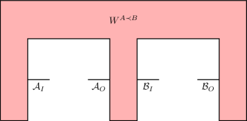
Figure 1. A schematic representation of a process matrix $W^{A\prec B}$ representing a quantum comb $A\prec B$.

One can easily observe that the set $\mathbf{W^{A||B}}$ is an intersection of the sets $\mathbf{W^{A\prec B}}$ and $\mathbf{W^{B\prec A}}$. Finally, the definition of the set $\mathbf{W^{A\prec B}}$, together with $\mathbf{W^{B\prec A}}$ allow us to provide their convex hull which is called as causally separable process matrices.

Definition 5.

We say that $W^{SEP}\in\mathbf{W^{PROC}}$ is a causally separable process matrix if it is of the form

$$W^{\text{SEP}}=pW^{A\prec B}+(1-p)W^{B\prec A},$$ (18)

where $W^{A\prec B}\in\mathbf{W^{A\prec B}}$, $W^{B\prec A}\in\mathbf{W^{B\prec A}}$ for some parameter $p\in[0,1]$. The set of all causally separable process matrices will be denoted by $\mathbf{W^{SEP}}$.

There are however process matrices that do not correspond to a causally separable process and such process matrices are known as causally non-separable (CNS). The examples of such matrices were provided in [5, 28]. The set of all causally non-separable process matrices will be denoted by $\mathbf{W^{CNS}}$. In Fig. 2 we present a schematic plot of the sets of process matrices.

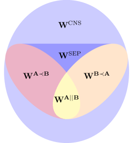
Figure 2. A schematic representation of the sets of process matrices $\mathbf{W^{PROC}}$.

4. Discrimination task

This section presents the concept of discrimination between pairs of process matrices. It is worth emphasizing that the definition of a process matrix is a generalization of the concept of quantum states, channels, superchannels [29] and even generalized supermaps [30, 31]. The task of discrimination between process matrices poses a natural extension of discrimination of quantum states [32], channels [33] or measurements [13]. The process matrices discrimination task can be described by the following scenario.

Let us consider two process matrices $W_{0},W_{1}\in\mathbf{W^{PROC}}$. The classical description of process matrices $W_{0},W_{1}$ is assumed to be known to the participating parties. We know that one of the process matrices, $W_{0}$ or $W_{1}$, describes the actual correlation between Alice’s and Bob’s laboratories, but we do not know which one. Our aim is to determine, with the highest possible probability, which process matrix describes this correlation. For this purpose, we construct a discrimination strategy $S$. In the general approach, such a strategy $S$ is described by an instrument $S=\{S_{0},S_{1}\}$. Due to the requirement given by Eq. (14), the instrument $S$ must fulfill the condition $S_{0}+S_{1}\in\mathbf{NS}(\mathcal{A}_{I}\otimes\mathcal{A}_{O}\otimes\mathcal{B}_{I}\otimes\mathcal{B}_{O})$. The result of composing a process matrix $W$ with the discrimination strategy $S$ results in a classical label which can take values zero or one. If the label zero occurs, we decide to choose that the correlation is given by $W_{0}$. Otherwise, we decide to choose $W_{1}$. In this setting the maximum success probability $p_{\text{succ}}(W_{0},W_{1})$ of correct discrimination between two process matrices $W_{0}$ and $W_{1}$ can be expressed by

$$p_{\text{succ}}(W_{0},W_{1})=\frac{1}{2}\max_{S=\{S_{0},S_{1}\}}\left[\operatorname{tr}(W_{0}S_{0})+\operatorname{tr}(W_{1}S_{1})\right].$$ (19)

The following theorem provides the optimal probability of process matrices discrimination as a direct analogue of the Holevo–Helstrom theorem for quantum states and channels.

Theorem 1.

Let $W_{0},W_{1}\in\mathbf{W^{PROC}}$ be two process matrices. For every choice of discrimination strategy $S=\{S_{0},S_{1}\}$, it holds that

$$\begin{split}&\frac{1}{2}\operatorname{tr}(S_{0}W_{0})+\frac{1}{2}\operatorname{tr}(S_{1}W_{1})\leq\\ &\frac{1}{2}+\frac{1}{4}\max\left\{\|\sqrt{N}(W_{0}-W_{1})\sqrt{N}\|_{1}:N\in\mathbf{NS}(\mathcal{A}_{I}\otimes\mathcal{A}_{O}\otimes\mathcal{B}_{I}\otimes\mathcal{B}_{O})\right\},\end{split}$$ (20)

where $\mathbf{NS}(\mathcal{A}_{I}\otimes\mathcal{A}_{O}\otimes\mathcal{B}_{I}\otimes\mathcal{B}_{O})$ is the set of Choi matrices of non-signaling channels. Moreover, there exists a discrimination strategy $S$, which saturates the inequality Eq. (20).

Proof.

Let us define the sets

$$\mathbf{A}\coloneqq\left\{(S_{0},S_{1}):S_{0}+S_{1}\in\mathbf{NS}(\mathcal{A}_{I}\otimes\mathcal{A}_{O}\otimes\mathcal{B}_{I}\otimes\mathcal{B}_{O}),\,\,S_{0},\,S_{1}\geq 0\right\}.$$ (21)

and

$$\begin{split}\mathbf{B}\coloneqq\{(\sqrt{N}Q_{0}\sqrt{N},\sqrt{N}Q_{1}\sqrt{N}):&\,N\in\mathbf{NS}(\mathcal{A}_{I}\otimes\mathcal{A}_{O}\otimes\mathcal{B}_{I}\otimes\mathcal{B}_{O}),\\ &Q_{0},\,Q_{1}\geq 0,\\ &Q_{0}+Q_{1}={\rm 1l}_{\mathcal{A}_{I}\mathcal{A}_{O}\mathcal{B}_{I}\mathcal{B}_{O}}\}.\end{split}$$ (22)

We prove the equality between sets $\mathbf{A}$ and $\mathbf{B}$. To show $\mathbf{B}\subseteq\mathbf{A}$, it is suffices to observe that $\sqrt{N}Q_{0}\sqrt{N}+\sqrt{N}Q_{1}\sqrt{N}\in\mathbf{NS}(\mathcal{A}_{I}\otimes\mathcal{A}_{O}\otimes\mathcal{B}_{I}\otimes\mathcal{B}_{O})$. To prove $\mathbf{A}\subseteq\mathbf{B}$ let us take $N\coloneqq S_{0}+S_{1}$. It implies that

$$\Pi_{\text{im}(N)}=\sqrt{N}^{-1}N\sqrt{N}^{-1}=\sqrt{N}^{-1}S_{0}\sqrt{N}^{-1}+\sqrt{N}^{-1}S_{1}\sqrt{N}^{-1}.$$ (23)

Let us fix $\widetilde{Q_{0}}\coloneqq\sqrt{N}^{-1}S_{0}\sqrt{N}^{-1}$ and $\widetilde{Q_{1}}\coloneqq\sqrt{N}^{-1}S_{1}\sqrt{N}^{-1}$. Then, we have ${\rm 1l}_{\mathcal{A}_{I}\mathcal{A}_{O}\mathcal{B}_{I}\mathcal{B}_{O}}={\rm 1l}_{\mathcal{A}_{I}\mathcal{A}_{O}\mathcal{B}_{I}\mathcal{B}_{O}}-\Pi_{\text{im}(N)}+\Pi_{\text{im}(N)}={\rm 1l}_{\mathcal{A}_{I}\mathcal{A}_{O}\mathcal{B}_{I}\mathcal{B}_{O}}-\Pi_{\text{im}(N)}+\widetilde{Q_{0}}+\widetilde{Q_{1}}$. Finally, it is suffices to take

$$Q_{0}\coloneqq{\rm 1l}_{\mathcal{A}_{I}\mathcal{A}_{O}\mathcal{B}_{I}\mathcal{B}_{O}}-\Pi_{\text{im}(N)}+\widetilde{Q_{0}}$$ (24)

and $Q_{1}\coloneqq\widetilde{Q_{1}}$. It implies that $\mathbf{A}=\mathbf{B}$. In conclusion, we obtain

$$\begin{split}&\frac{1}{2}\operatorname{tr}(S_{0}W_{0})+\frac{1}{2}\operatorname{tr}(S_{1}W_{1})\\ &=\frac{1}{2}\operatorname{tr}\left(\sqrt{N}Q_{0}\sqrt{N}W_{0}\right)+\frac{1}{2}\operatorname{tr}\left(\sqrt{N}Q_{1}\sqrt{N}W_{1}\right)\\ &=\frac{1}{2}\operatorname{tr}\left(Q_{0}\sqrt{N}W_{0}\sqrt{N}\right)+\frac{1}{2}\operatorname{tr}\left(Q_{1}\sqrt{N}W_{1}\sqrt{N}\right)\\ &\leq\frac{1}{2}+\frac{1}{4}\max\left\{||\sqrt{N}(W_{0}-W_{1})\sqrt{N}||_{1}:N\in\mathbf{NS}(\mathcal{A}_{I}\otimes\mathcal{A}_{O}\otimes\mathcal{B}_{I}\otimes\mathcal{B}_{O})\right\}.\end{split}$$ (25)

Moreover, from Holevo-Helstrom theorem [33] there exists a projective binary measurement $Q=\{Q_{0},Q_{1}\}$ such that the last inequality is saturated, which completes the proof. ∎

Corollary 1.

The maximum probability $p_{\text{succ}}(W_{0},W_{1})$ of correct discrimination between two process matrices $W_{0}$ and $W_{1}$ is given by

$$\begin{split}&p_{\text{succ}}(W_{0},W_{1})=\\ &\frac{1}{2}+\frac{1}{4}\max\left\{\|\sqrt{N}(W_{0}-W_{1})\sqrt{N}\|_{1}:N\in\mathbf{NS}(\mathcal{A}_{I}\otimes\mathcal{A}_{O}\otimes\mathcal{B}_{I}\otimes\mathcal{B}_{O})\right\}.\end{split}$$ (26)

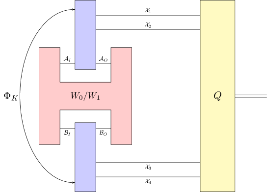
Figure 3. A schematic representation of the setup for distinguishing between process matrices $W_{0}$ and $W_{1}$. The discrimination strategy is constructed by using the quantum channel $\Phi_{K}:\mathrm{L}(\mathcal{A}_{I}\otimes\mathcal{B}_{I})\rightarrow\mathrm{L}(\mathcal{A}_{O}\otimes\mathcal{B}_{O}\otimes\mathcal{X}_{1}\otimes\mathcal{X}_{2}\otimes\mathcal{X}_{3}\otimes\mathcal{X}_{4})$ and the binary measurement $Q=\{Q_{0},Q_{1}\}$ defined in the proof of Theorem 1.

As a valuable by-product of Theorem 1, we receive a realization of process matrices discrimination scheme. The schematic representation of this setup is presented in Fig. 3. To distinguish the process matrices $W_{0}$ and $W_{1}$, Alice and Bob prepare the strategy $S=\{S_{0},S_{1}\}$ such that $S_{0}+S_{1}\in\mathbf{NS}(\mathcal{A}_{I}\otimes\mathcal{A}_{O}\otimes\mathcal{B}_{I}\otimes\mathcal{B}_{O})$. To implement it, let us introduce complex Euclidean spaces $\mathcal{X}_{1},\ldots,\mathcal{X}_{4}$ such that $\dim\left(\bigotimes_{i=1}^{4}\mathcal{X}_{i}\right)=\dim(\mathcal{A}_{I}\otimes\mathcal{A}_{O}\otimes\mathcal{B}_{I}\otimes\mathcal{B}_{O})$. Alice and Bob prepare the quantum channel $\Phi_{K}:\mathrm{L}(\mathcal{A}_{I}\otimes\mathcal{B}_{I})\rightarrow\mathrm{L}(\mathcal{A}_{O}\otimes\mathcal{B}_{O}\otimes\mathcal{X}_{1}\otimes\mathcal{X}_{2}\otimes\mathcal{X}_{3}\otimes\mathcal{X}_{4})$ with the Choi matrix $K$ given by

$$K=\left({\rm 1l}_{\mathcal{X}_{1,2,3,4}}\otimes\sqrt{N}\right)\left(|{\rm 1l}\rangle\rangle\langle\langle{\rm 1l}|\right)\left({\rm 1l}_{\mathcal{X}_{1,2,3,4}}\otimes\sqrt{N}\right),$$ (27)

where $|{\rm 1l}\rangle\rangle\in\mathrm{L}(\mathcal{X}_{1}\otimes\mathcal{X}_{2}\otimes\mathcal{X}_{3}\otimes\mathcal{X}_{4}\otimes\mathcal{A}_{I}\otimes\mathcal{A}_{O}\otimes\mathcal{B}_{I}\otimes\mathcal{B}_{O})$ and $N\in\mathbf{NS}(\mathcal{A}_{I}\otimes\mathcal{A}_{O}\otimes\mathcal{B}_{I}\otimes\mathcal{B}_{O})$ maximizes the trace norm $\|\sqrt{N}(W_{0}-W_{1})\sqrt{N}\|_{1}$. It is worth noting that the quantum channel $\Phi_{K}$ is correctly defined due to the fact that $\operatorname{tr}_{\mathcal{X}_{1,2,3,4}}K\in\mathbf{NS}(\mathcal{A}_{I}\otimes\mathcal{A}_{O}\otimes\mathcal{B}_{I}\otimes\mathcal{B}_{O})$. Afterwards, they perform the binary measurement $Q=\{Q_{0},Q_{1}\}$, where the effect $Q_{0}\in\mathrm{L}(\mathcal{X}_{1}\otimes\mathcal{X}_{2}\otimes\mathcal{X}_{3}\otimes\mathcal{X}_{4})$ is defined by Eq. (24). Next, they decide which process matrix was used during the calculation assuming $W_{0}$ if the measurement label is $0$. Otherwise, they assume $W_{1}$.

5. Discrimination between different classes of process matrices

This section presents some examples of discrimination between different classes of process matrices. We begin our consideration with the problem of discrimination between two free process matrices $\mathbf{W^{A||B}}$. Next, we will consider various cases of process matrices discrimination representing a quantum comb. First, we calculate exact probability of correct discrimination between two process matrices come from the same class $\mathbf{W^{A\prec B}}$. Next, we study the discrimination task assuming that one of the process matrices is of the form $\mathbf{W^{A\prec B}}$ and the other one is of the form $\mathbf{W^{B\prec A}}$. Finally, we construct a particular class of process matrices which can be perfectly distinguished.

5.1. Free process matrices

The following consideration confirms an intuition that the task of discrimination between free process matrices reduces to the problem of discrimination between quantum states.

From definition of $p_{\text{succ}}(W_{0},W_{1})$ we have

$$\begin{split}p_{\text{succ}}\left(W_{0},W_{1}\right)=\frac{1}{2}\max_{S=\{S_{0}, S_{1}\}}\left[\operatorname{tr}\left(W_{0}S_{0}\right)+\operatorname{tr}\left(W_{1}S_{1}\right)\right],\end{split}$$ (28)

Let $W_{0}$ and $W_{1}$ be two process matrices of the form $W_{0}=\rho\otimes{\rm 1l}_{\mathcal{A}_{O}\mathcal{B}_{O}}$ and $W_{1}=\sigma\,\otimes\,{\rm 1l}_{\mathcal{A}_{O}\mathcal{B}_{O}}$, where $\rho,\,\sigma\in\Omega(\mathcal{A}_{I}\otimes\mathcal{B}_{I})$. Then, $p_{\text{succ}}$ is exactly equal to

$$\begin{split}&\max_{S=\{S_{0},S_{1}\}}\left[\frac{1}{2}\operatorname{tr}\left(W_{0}S_{0}\right)+\frac{1}{2}\operatorname{tr}\left(W_{1}S_{1}\right)\right]=\\ &\max_{S=\{S_{0},S_{1}\}}\left[\frac{1}{2}\operatorname{tr}\left((\rho\otimes{\rm 1l})S_{0}\right)+\frac{1}{2}\operatorname{tr}\left((\sigma\otimes{\rm 1l})S_{1}\right)\right]=\\ &\max_{S=\{S_{0},S_{1}\}}\left[\frac{1}{2}\operatorname{tr}\left(\rho\operatorname{tr}_{\mathcal{A}_{O}\mathcal{B}_{O}}S_{0}\right)+\frac{1}{2}\operatorname{tr}\left(\sigma\operatorname{tr}_{\mathcal{A}_{O}\mathcal{B}_{O}}S_{1}\right)\right].\end{split}$$ (29)

Let us observe $\operatorname{tr}_{\mathcal{A}_{O}\mathcal{B}_{O}}S_{0}+\operatorname{tr}_{\mathcal{A}_{O}\mathcal{B}_{O}}S_{1}={\rm 1l}_{\mathcal{A}_{I}\mathcal{B}_{I}}$. So, $\{\operatorname{tr}_{\mathcal{A}_{O}\mathcal{B}_{O}}S_{0},\operatorname{tr}_{\mathcal{A}_{O}\mathcal{B}_{O}}S_{1}\}$ is a binary measurement and therefore, from Holevo-Helstrom theorem for quantum states, we have

$$\max_{S=\{S_{0},S_{1}\}}\left[\frac{1}{2}\operatorname{tr}\left(\rho\operatorname{tr}_{\mathcal{A}_{O}\mathcal{B}_{O}}S_{0}\right)+\frac{1}{2}\operatorname{tr}\left(\sigma\operatorname{tr}_{\mathcal{A}_{O}\mathcal{B}_{O}}S_{1}\right)\right]\leq\frac{1}{2}+\frac{1}{4}\|\rho-\sigma\|_{1}.$$ (30)

Now, assume that $E=\{E_{0},E_{1}\}$ is the Holevo-Helstrom measurement (by taking $E_{0}$ and $E_{1}$ as positive and negative part of $\rho-\sigma$, respectively). Hence, we obtain

$$\max_{E=\{E_{0},E_{1}\}}\left[\frac{1}{2}\operatorname{tr}\left(\rho E_{0}\right)+\frac{1}{2}\operatorname{tr}\left(\sigma E_{1}\right)\right]=\frac{1}{2}+\frac{1}{4}\|\rho-\sigma\|_{1}.$$ (31)

Observe, it is suffices to take $S_{0}\coloneqq E_{0}\otimes|0\rangle\!\langle 0|\otimes|0\rangle\!\langle 0|$ and $S_{1}\coloneqq E_{1}\otimes|0\rangle\!\langle 0|\otimes|0\rangle\!\langle 0|$. Note that $S_{0}+S_{1}={\rm 1l}_{\mathcal{A}_{I}\mathcal{B}_{I}}\otimes|0\rangle\!\langle 0|\otimes|0\rangle\!\langle 0|$ is non-signaling channel. Therefore, we have

$$p_{\text{succ}}\left(W_{0},W_{1}\right)=\frac{1}{2}+\frac{1}{4}\|\rho-\sigma\|_{1}.$$ (32)

which completes the consideration.

Due to the above consideration, we obtain the following corollary.

Corollary 2.

Let $\rho,\sigma\in\Omega(\mathcal{A}_{I}\otimes\mathcal{B}_{I})$ be quantum states and let $W_{0},W_{1}\in\mathbf{W^{A||B}}$ be two free process matrices of the form $W_{0}=\rho\otimes{\rm 1l}$ and $W_{1}=\sigma\otimes{\rm 1l}$. Then,

$$p_{\text{succ}}\left(W_{0},W_{1}\right)=\frac{1}{2}+\frac{1}{4}\|\rho-\sigma\|_{1}.$$ (33)

5.2. Process matrices representing quantum combs

Here, we will compare the probability of correct discrimination between two process matrices being quantum combs of the form $W_{0}^{A\prec B},W_{1}^{A\prec B}\in\mathbf{W^{A\prec B}}$ by using non-signalling strategy $S=\{S_{0},S_{1}\}$ described by Eq. (54) or an adaptive strategy.

Before that, we will discuss the issue of adaptive strategy. The most general strategy of quantum operations discrimination is known as an adaptive strategy [34, 19]. An adaptive strategy is realized by a quantum tester [1]. A schematic representation of this setup is presented in Fig. 4.

Let us consider a quantum tester $\{L_{0},L_{1}\}$. The probability of correct discrimination between $W_{0}^{A\prec B}$ and $W_{1}^{A\prec B}$ by using an adaptive strategy is defined by equation

$$p_{adapt}\left(W_{0}^{A\prec B},W_{1}^{A\prec B}\right)\coloneqq\frac{1}{2}\max_{\{L_{0},L_{1}\}}L_{0}*W_{0}+L_{1}*W_{1}.$$ (34)

Figure 4. A schematic representation of an adaptive strategy discriminating two process matrices $W_{0},W_{1}\in W^{A\prec B}$ by using a quantum tester $\{L_{0},L_{1}\}$.

It turns out that we do not need adaptation in order to obtain the optimal probability os distinction. This is stated formally in the following theorem.

Theorem 2.

Let $W_{0}^{A\prec B},W_{1}^{A\prec B}\in\mathbf{W^{A\prec B}}$ be two process matrices representing quantum combs $A\prec B$. Then,

$$p_{succ}\left(W_{0}^{A\prec B},W_{1}^{A\prec B}\right)=p_{adapt}\left(W_{0}^{A\prec B},W_{1}^{A\prec B}\right).$$ (35)

Proof.

For simplicity, we will omit superscripts ($A\prec B$ and $B\prec A$). The inequality $p_{succ}\left(W_{0},W_{1}\right)\leq p_{adapt}\left(W_{0},W_{1}\right)$ is trivial by observing that we calculate maximum value over a larger set.

To show $p_{succ}\left(W_{0},W_{1}\right)\geq p_{adapt}\left(W_{0},W_{1}\right)$, let us consider the quantum tester $\{L_{0},L_{1}\}$ which maximizes Eq. (34), that means

$$p_{adapt}\left(W_{0},W_{1}\right)=\frac{1}{2}\left(L_{0}*W_{0}+L_{1}*W_{1}\right).$$ (36)

Hence, from definition of $W^{A\prec B}$ we have

$$W^{A\prec B}=W^{\prime}\otimes{\rm 1l}_{\mathcal{B}_{O}},$$ (37)

and then we obtain

$$\frac{1}{2}\left(L_{0}*W_{0}+L_{1}*W_{1}\right)=\frac{1}{2}\operatorname{tr}\left(W^{\prime}_{0}\operatorname{tr}_{\mathcal{B}_{O}}L_{0}+W^{\prime}_{1}\operatorname{tr}_{\mathcal{B}_{O}}L_{1}\right).$$ (38)

Observe that $\operatorname{tr}_{\mathcal{B}_{O}}(L_{0}+L_{1})={\rm 1l}_{\mathcal{B}_{I}}\otimes J$, where $J$ is a Choi matrix of a channel $\Phi_{J}:\mathrm{L}(\mathcal{A}_{I})\rightarrow\mathrm{L}(\mathcal{A}_{O})$. Let us define a strategy $S=\{S_{0},S_{1}\}$ such that

$$\begin{split}&S_{0}=\operatorname{tr}_{\mathcal{B}_{O}}L_{0}\otimes\frac{{\rm 1l}_{\mathcal{B}_{O}}}{\dim(\mathcal{B}_{O})},\\ &S_{1}=\operatorname{tr}_{\mathcal{B}_{O}}L_{1}\otimes\frac{{\rm 1l}_{\mathcal{B}_{O}}}{\dim(\mathcal{B}_{O})},\\ &S=S_{0}+S_{1}.\end{split}$$ (39)

It easy to observe that $S\in\mathbf{NS}(\mathcal{A}_{O}\otimes\mathcal{A}_{I}\otimes\mathcal{B}_{O}\otimes\mathcal{B}_{I})$. Then, we have

$$\frac{1}{2}\left(S_{0}*W_{0}+S_{1}*W_{1}\right)=\frac{1}{2}\left(\operatorname{tr}\left(W^{\prime}_{0}\operatorname{tr}_{\mathcal{B}_{O}}L_{0}+W^{\prime}_{1}\operatorname{tr}_{\mathcal{B}_{O}}L_{1}\right)\right).$$ (40)

It implies that

$$p_{succ}\left(W_{0},W_{1}\right)\geq p_{adapt}\left(W_{0},W_{1}\right),$$ (41)

which completes the proof. ∎

5.3. Process matrices of the form $W^{A\prec B}$ and $W^{B\prec A}$

Now, we present some results for discrimination task assuming the one of the process matrices if of the form $\mathbf{W^{A\prec B}}$ and the other one is of the form $\mathbf{W^{B\prec A}}$. We will construct a particular class of such process matrices for which the perfect discrimination is possible.

Let us define a process matrix of the form

$$W^{A\prec B}=\rho\otimes|U\rangle\rangle\langle\langle U|\otimes{\rm 1l},$$ (42)

where $\rho\in\Omega(\mathcal{A}_{I}),|U\rangle\rangle\langle\langle U|$ is the Choi matrix of a unitary channel $\mathrm{Ad}_{U^{\top}}:\mathrm{L}(\mathcal{A}_{O})\rightarrow\mathrm{L}(\mathcal{B}_{I})$ of the form $\mathrm{Ad}_{U^{\top}}(X)=U^{\top}X\,\bar{U}$ and ${\rm 1l}\in\mathrm{L}(\mathcal{B}_{O})$. A schematic representation of this process matrix we can see in Fig. 5.

Figure 5. A schematic representation of process matrix $W^{A\prec B}$ given by Eq. (42).

Proposition 1.

Let $W^{A\prec B}$ be a process matrix given by Eq. (42). Let us define a process matrix $W^{B\prec A}$ of the form

$$W^{B\prec A}=P_{\pi}W^{A\prec B}P_{\pi},$$ (43)

where $P_{\pi}$ is the swap operator replacing the systems $\mathcal{A}_{I}\rightarrow\mathcal{B}_{I}$ and $\mathcal{A}_{O}\rightarrow\mathcal{B}_{O}$. Then, the process matrix $W^{A\prec B}$ is perfectly distinguishable from $W^{B\prec A}$.

Proof.

Let us consider the process matrix given by Eq. (42) described by Fig. 5. W.l.o.g. let $d$ be a dimension of each of the systems. Let $\rho=\sum_{i=0}^{d-1}\lambda_{i}|x_{i}\rangle\!\langle x_{i}|$, where $\lambda_{i}\geq 0$ such that $\sum_{i}\lambda_{i}=1$. Based on the spectral decomposition of $\rho$ we create the unitary matrix $V$ by taking $i$-th eigenvector of $\rho$, and the measurement $\Delta_{V}$ (in basis of $\rho$) given by

$$\Delta_{V}(X)=\sum_{i=0}^{d-1}\langle x_{i}|X|x_{i}\rangle|i\rangle\!\langle i|\otimes|x_{i}\rangle\!\langle x_{i}|.$$ (44)

Let us also define the permutation matrix $P_{\sigma}=\sum_{i=0}^{d-1}|x_{{i+1}\text{ mod d}}\rangle\!\langle x_{i}|$ corresponding to the permutation $\sigma=(0,1,\ldots,d-1)$.

Alice and Bob prepare theirs discrimination strategy. Alice performs the local channel (see Fig. 6) given by

$$\Phi_{A}(\rho)=\left(\left(\mathcal{I}\otimes\mathrm{Ad}_{\bar{U}}\right)\circ\Delta_{V}\right)(\rho),$$ (45)

Meanwhile, Bob performs his local channel (see Fig. 7) given by

$$\Phi_{B}(\rho)=\left(\left(\mathcal{I}\otimes\mathrm{Ad}_{\bar{U}}\right)\circ\Delta_{V}\circ\mathrm{Ad}_{P_{\sigma}}\right)(\rho).$$ (46)

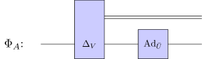
Figure 6. A schematic representation of Alice’s discrimination strategy described by Eq. (45).

Figure 7. A schematic representation of Bobs’ discrimination strategy described by Eq. (46).

Let us consider the case $A\prec B$. The output after Alice’s action is described by

$$\Phi_{A}(\rho)=\sum_{i}\lambda_{i}|i\rangle\!\langle i|\otimes\bar{U}|x_{i}\rangle\!\langle x_{i}|U^{\top}.$$ (47)

Next, we apply the quantum channel $\mathrm{Ad}_{U^{\top}}$ (see Fig.5), and hence we have

$$(\mathcal{I}\otimes\mathrm{Ad}_{U^{\top}})\circ\Phi_{A}(\rho)=\sum_{i}\lambda_{i}|i\rangle\!\langle i|\otimes|x_{i}\rangle\!\langle x_{i}|.$$ (48)

In the next step, Bob applies his channel as follows

$$(\mathcal{I}\otimes\Phi_{B})\circ(\mathcal{I}\otimes\mathrm{Ad}_{U^{\top}})\circ\Phi_{A}(\rho)=\sum_{i}\lambda_{i}|i\rangle\!\langle i|\otimes|i+1\rangle\!\langle i+1|\otimes|x_{i+1}\rangle\!\langle x_{i+1}|.$$ (49)

Finally, we apply partial trace operation on the subspace $\mathcal{B}_{O}$ (see Fig.5), that means

$$\operatorname{tr}_{\mathcal{B}_{O}}\left(\sum_{i}\lambda_{i}|i\rangle\!\langle i|\otimes|i+1\rangle\!\langle i+1|\otimes|x_{i+1}\rangle\!\langle x_{i+1}|\right)=\sum_{i}\lambda_{i}|i\rangle\!\langle i|\otimes|i+1\rangle\!\langle i+1|.$$ (50)

So, the quantum state obtained after the discrimination scenario in the case $A\prec B$ is given by

$$\sigma^{A\prec B}=\sum_{i}\lambda_{i}|i\rangle\!\langle i|\otimes|i+1\rangle\!\langle i+1|.$$ (51)

It implies that if Alice measures her system, she obtains the label $i$ with probability $\lambda_{i}$ whereas Bob obtains the label $(i+1)\mod d$ with the same probability. On the other hand, considering the case $B\prec A$, then the state obtained after the discrimination scenario is given by

$$\sigma^{B\prec A}=\sum_{i}\lambda_{i}|i+1\rangle\!\langle i+1|\otimes|i+1\rangle\!\langle i+1|.$$ (52)

So, Bob and Alice obtain the same label $(i+1)\mod d$ with probability $\lambda_{i}$. Then, the quantum channel $\Phi_{K}$ (realizing the discrimination strategy $S$) is created as a tensor product of Alice’s and Bob’s local channels, that means $\Phi_{K}=\Phi_{A}\otimes\Phi_{B}$. Due to that they perform the binary measurement $Q=\{Q_{0},Q_{1}\}$, where the effect $Q_{1}$ is given by $Q_{1}=\sum_{i=0}^{d-1}|i\rangle\!\langle i|\otimes|i\rangle\!\langle i|$. Hence, we have

$$p_{\text{succ}}(W^{A\prec B},W^{B\prec A})=\frac{1}{2}\operatorname{tr}\left(\sigma^{A\prec B}Q_{0}\right)+\frac{1}{2}\operatorname{tr}\left(\sigma^{B\prec A}Q_{1}\right)=1.$$ (53)

In summary, the process matrices $W^{A\prec B}$ and $W^{B\prec A}$ are perfectly distinguishable by Alice and Bob which completes the proof.

∎

6. SDP program for calculating the optimal probability of process matrices discrimination

In the standard approach, we would need to compute the probability of correct discrimination between two process matrices $W_{0}$ and $W_{1}$. For this purpose, we use the semidefinite programming (SDP). This section presents the SDP program for calculating the optimal probability of discrimination between $W_{0}$ and $W_{1}$.

Recall that the maximum value of such a probability can be noticed by

$$p_{\text{succ}}(W_{0},W_{1})=\frac{1}{2}\max_{S=\{S_{0},S_{1}\}}\left[\operatorname{tr}(W_{0}S_{0})+\operatorname{tr}(W_{1}S_{1})\right],$$ (54)

with requirement that the optimal strategy $S=\{S_{0},S_{1}\}$ is a quantum instrument such that $S_{0}+S_{1}\in\mathbf{NS}(\mathcal{A}_{I}\otimes\mathcal{A}_{O}\otimes\mathcal{B}_{I}\otimes\mathcal{B}_{O})$. Hence, we arrive at the primal and dual problems presented in the Program 1. To optimize this problem we used the Julia programming language along with quantum package QuantumInformation.jl[35] and SDP optimization via SCS solver [36, 37] with absolute convergence tolerance $10^{-5}$. The code is available on GitHub [38].

It may happen that the values of primal and dual programs are equal. This situation is called strong duality. Slater’s theorem provides the set of conditions which guarantee strong duality [33]. It can be shown that Program 1 fulfills conditions of Slater’s theorem (it is suffices to take $Y_{0},Y_{1}=0$ and $\alpha>\frac{1}{2}\max\{\Lambda^{\text{max}}(W_{0}),\Lambda^{\text{max}}(W_{1})\}$, where $\Lambda^{\text{max}}(X)$ is the maximum eigenvalue of $X$). Therefore, we can consider the primal and the dual problem equivalently.

SDP program for calculating the optimal probability of discrimination between $W_{0}$ and $W_{1}$

Primal problem

$$\begin{split}\text{maximize:}\quad&\frac{1}{2}\operatorname{Tr}(W_{0}S_{0})+\frac{1}{2}\operatorname{Tr}(W_{1}S_{1})\\[5.69054pt] \text{subject to:}\quad&\operatorname{tr}_{\mathcal{A}_{O}}(S_{0}+S_{1})=\frac{{\rm 1l}_{\mathcal{A}_{I}}}{\dim(\mathcal{A}_{I})}\otimes\operatorname{tr}_{\mathcal{A}_{O}\mathcal{A}_{I}}(S_{0}+S_{1}),\\ &\operatorname{tr}_{\mathcal{B}_{O}}(S_{0}+S_{1})=\frac{{\rm 1l}_{\mathcal{B}_{I}}}{\dim(\mathcal{B}_{I})}\otimes\operatorname{tr}_{\mathcal{B}_{O}\mathcal{B}_{I}}(S_{0}+S_{1}),\\ &\operatorname{tr}(S_{0}+S_{1})=\dim(\mathcal{A}_{I})\dim(\mathcal{B}_{I}),\\ &S_{0}\in\mathrm{Pos}(\mathcal{A}_{I}\otimes\mathcal{A}_{O}\otimes\mathcal{B}_{I}\otimes\mathcal{B}_{O}),\\ &S_{1}\in\mathrm{Pos}(\mathcal{A}_{I}\otimes\mathcal{A}_{O}\otimes\mathcal{B}_{I}\otimes\mathcal{B}_{O}).\end{split}$$

Dual problem

$$\begin{split}\text{minimize:}\quad&\alpha\cdot\dim(\mathcal{A}_{I})\dim(\mathcal{B}_{I})\\[5.69054pt] \text{subject to:}\quad&{\rm 1l}_{\mathcal{A}_{O}}\otimes Y_{0}-\frac{{\rm 1l}_{\mathcal{A}_{I}\mathcal{A}_{O}}}{\dim(\mathcal{A}_{I})}\otimes\operatorname{tr}_{\mathcal{A}_{I}}(Y_{0})+{\rm 1l}_{\mathcal{B}_{O}}\otimes Y_{1}+\\ &-\frac{{\rm 1l}_{\mathcal{B}_{I}\mathcal{B}_{O}}}{\dim(\mathcal{B}_{I})}\otimes\operatorname{tr}_{\mathcal{B}_{I}}Y_{1}+\alpha\cdot{\rm 1l}_{\mathcal{A}_{I}\mathcal{A}_{O}\mathcal{B}_{I}\mathcal{B}_{O}}\geq\frac{1}{2}W_{0},\\ &{\rm 1l}_{\mathcal{A}_{O}}\otimes Y_{0}-\frac{{\rm 1l}_{\mathcal{A}_{I}\mathcal{A}_{O}}}{\dim(\mathcal{A}_{I})}\otimes\operatorname{tr}_{\mathcal{A}_{I}}(Y_{0})+{\rm 1l}_{\mathcal{B}_{O}}\otimes Y_{1}+\\ &-\frac{{\rm 1l}_{\mathcal{B}_{I}\mathcal{B}_{O}}}{\dim(\mathcal{B}_{I})}\otimes\operatorname{tr}_{\mathcal{B}_{I}}Y_{1}+\alpha\cdot{\rm 1l}_{\mathcal{A}_{I}\mathcal{A}_{O}\mathcal{B}_{I}\mathcal{B}_{O}}\geq\frac{1}{2}W_{1},\\ &Y_{0}\in\text{ Herm}(\mathcal{A}_{I}\otimes\mathcal{B}_{I}\otimes\mathcal{B}_{O}),\\ &Y_{1}\in\text{ Herm}(\mathcal{A}_{I}\otimes\mathcal{A}_{O}\otimes\mathcal{B}_{I}),\\ &\alpha\in\mathbb{R}.\end{split}$$

Table 1. Semidefinite program for maximizing the probability of correct discrimination between two process matrices $W_{0}$ and $W_{1}$.

7. Distance between process matrices

In this section we present the semidefinite programs for calculating the distance in trace norm between a given process matrix $W\in\mathbf{W^{PROC}}$ and different subsets of process matrices, such that $\mathbf{W^{A||B}}$ , $\mathbf{W^{A\prec B}}$, $\mathbf{W^{B\prec A}}$ or $\mathbf{W^{SEP}}$.

For example, let us consider the case $\mathbf{W^{A||B}}$. Theoretically, the distance between a process matrix $W$ and the set of free process matrices $\mathbf{W^{A||B}}$ can be expressed by

$$\begin{split}&\text{dist}\left(W,\mathbf{W^{A||B}}\right)=\\ &\min_{\widetilde{W}\in\mathbf{W^{A||B}}}\max\left\{\|\sqrt{N}(W-\widetilde{W})\sqrt{N}\|_{1}:N\in\mathbf{NS}(\mathcal{A}_{I}\otimes\mathcal{A}_{O}\otimes\mathcal{B}_{I}\otimes\mathcal{B}_{O})\right\}.\end{split}$$ (55)

Analogously, for the sets $\mathbf{W^{A\prec B}},\mathbf{W^{B\prec A}}$ and $\mathbf{W^{SEP}}$ with the minimization condition $\min_{\widetilde{W}\in\mathbf{W^{A\prec B}}}$, $\min_{\widetilde{W}\in\mathbf{W^{B\prec A}}}$, $\min_{\widetilde{W}\in\mathbf{W^{SEP}}}$, respectively. Due to the results obtained from the previous section (see Program 1) and Slater theorem we are able to note the Eq. (55) to SDP problem presented in the Program 2. We use the SDP optimization via SCS solver [36, 37] with absolute convergence tolerance $10^{-8}$ and relative convergence tolerance $10^{-8}$. The implementations of SDPs in the Julia language are available on GitHub [38].

SDP calculating the distance between a process matrix $W$ and the set $\Upsilon$.

$$\begin{split}\text{minimize:}\quad&4\dim(\mathcal{A}_{I})\dim(\mathcal{B}_{I})\alpha-2\\[5.69054pt] \text{subject to:}\quad&{\rm 1l}_{\mathcal{A}_{O}}\otimes Y_{0}-\frac{{\rm 1l}_{\mathcal{A}_{I}\mathcal{A}_{O}}}{\dim(\mathcal{A}_{I})}\otimes\operatorname{tr}_{\mathcal{A}_{I}}(Y_{0})+{\rm 1l}_{\mathcal{B}_{O}}\otimes Y_{1}+\\ &-\frac{{\rm 1l}_{\mathcal{B}_{I}\mathcal{B}_{O}}}{\dim(\mathcal{B}_{I})}\otimes\operatorname{tr}_{\mathcal{B}_{I}}Y_{1}+\alpha\cdot{\rm 1l}_{\mathcal{A}_{I}\mathcal{A}_{O}\mathcal{B}_{I}\mathcal{B}_{O}}\geq\frac{1}{2}W,\\ &{\rm 1l}_{\mathcal{A}_{O}}\otimes Y_{0}-\frac{{\rm 1l}_{\mathcal{A}_{I}\mathcal{A}_{O}}}{\dim(\mathcal{A}_{I})}\otimes\operatorname{tr}_{\mathcal{A}_{I}}(Y_{0})+{\rm 1l}_{\mathcal{B}_{O}}\otimes Y_{1}+\\ &-\frac{{\rm 1l}_{\mathcal{B}_{I}\mathcal{B}_{O}}}{\dim(\mathcal{B}_{I})}\otimes\operatorname{tr}_{\mathcal{B}_{I}}Y_{1}+\alpha\cdot{\rm 1l}_{\mathcal{A}_{I}\mathcal{A}_{O}\mathcal{B}_{I}\mathcal{B}_{O}}\geq\frac{1}{2}W^{*},\\ &W^{*}\in\Upsilon,\\ &Y_{0}\in\text{ Herm}(\mathcal{A}_{I}\otimes\mathcal{B}_{I}\otimes\mathcal{B}_{O}),\\ &Y_{1}\in\text{ Herm}(\mathcal{A}_{I}\otimes\mathcal{A}_{O}\otimes\mathcal{B}_{I}),\\ &\alpha\in\mathbb{R}.\end{split}$$

Table 2. Semidefinite program for computation the distance between a process matrix $W$ and $\Upsilon$, which can be one of the set $\mathbf{W^{A||B}},\mathbf{W^{A\prec B}},\mathbf{W^{B\prec A}}$ or $\mathbf{W^{SEP}}$. Depending on the selected set we include additional constrains to SDP described by Eq. (16) for $\mathbf{W^{A||B}}$, Eq. (17) for $\mathbf{W^{A\prec B}}$ and $\mathbf{W^{B\prec A}}$ or Eq. (18) for $\mathbf{W^{SEP}}$.

7.1. Example

Let $\mathcal{A}_{I}=\mathcal{A}_{O}=\mathcal{B}_{I}=\mathcal{B}_{O}=\mathbb{C}^{2}$. Let us consider a causally non-separable process matrix comes from [5] of the form

$$W^{\text{CNS}}=\frac{1}{4}\left[{\rm 1l}_{\mathcal{A}_{I}\mathcal{A}_{O}\mathcal{B}_{I}\mathcal{B}_{O}}+\frac{1}{\sqrt{2}}\left(\sigma_{z}^{\mathcal{A}_{O}}\sigma_{z}^{\mathcal{B}_{I}}\otimes{\rm 1l}_{\mathcal{A}_{I}\mathcal{B}_{O}}+\sigma_{z}^{\mathcal{A}_{I}}\sigma_{x}^{\mathcal{B}_{I}}\sigma_{z}^{\mathcal{B}_{O}}\otimes{\rm 1l}_{\mathcal{A}_{O}}\right)\right],$$ (56)

where $\sigma_{x}^{\mathcal{X}},\sigma_{z}^{\mathcal{X}}$ are Pauli matrices on space $\mathrm{L}(\mathcal{X})$. We have calculated the distance in trace norm between $W^{\text{CNS}}$ and different subset of process matrices. Finally, we obtain

$$\text{dist}\left(W^{\text{CNS}},\mathbf{W^{A||B}}\right)\approx 1.00000001\approx 1,$$ (57)

$$\text{dist}\left(W^{\text{CNS}},\mathbf{W^{A\prec B}}\right)\approx 0.7071068\approx\frac{\sqrt{2}}{2},$$ (58)

$$\text{dist}\left(W^{\text{CNS}},\mathbf{W^{B\prec A}}\right)\approx 0.7071068\approx\frac{\sqrt{2}}{2},$$ (59)

$$\text{dist}\left(W^{\text{CNS}},\mathbf{W^{SEP}}\right)\approx 0.2928932\approx 1-\frac{\sqrt{2}}{2}.$$ (60)

The numerical computations give us some intuition about the geometry of the set of process matrices. Those results are presented in Fig. 8. Moreover, by using $W^{\text{CNS}}$ given by Eq. (56) it can be shown that the set of all causally non-separable process matrices is not convex. To show this fact, it suffices to observe that for every $\sigma_{i},\sigma_{j},\sigma_{k},\sigma_{l}\in\{\sigma_{x},\sigma_{y},\sigma_{z},{\rm 1l}\}$ the following equation holds

$$\left(\sigma_{i}\otimes\sigma_{j}\otimes\sigma_{k}\otimes\sigma_{l}\right)W^{\text{CNS}}(\sigma_{i}\otimes\sigma_{j}\otimes\sigma_{k}\otimes\sigma_{l})^{\dagger}\in\mathbf{W^{CNS}}.$$ (61)

Simultaneously, the average of the process matrices of the form Eq. (61) distributed uniformly states $\frac{1}{4}{\rm 1l}_{\mathbb{C}^{16}}$, however $\frac{1}{4}{\rm 1l}_{\mathbb{C}^{16}}\not\in\mathbf{W^{CNS}}$. It implies that the set $\mathbf{W^{CNS}}$ is not convex.

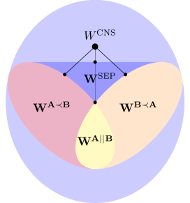
Figure 8. A schematic representation of the distances between $W^{\text{CNS}}$ defined in Eq. (56) and the sets $\mathbf{W^{A||B}}$, $\mathbf{W^{A\prec B}}$, $\mathbf{W^{B\prec A}}$ and $\mathbf{W^{SEP}}$.

8. Convex cone structure theory

From geometrical point of view, we present an alternative way to derive of Eq. (26). It turns out that the task of process matrices discrimination is strictly connected with the convex cone structure theory. To keep this work self-consistent, the details of convex cone structure theory are presented in Appendix A.

Let $\mathcal{V}$ be a finite dimensional real vector space with a proper cone $\mathcal{C}\subset\mathcal{V}$. A base $B$ of the proper cone $\mathcal{C}$ is a compact convex subset $B\subset\mathcal{C}$ such that each nonzero element $c\in\mathcal{C}$ has a unique representation in the form $c=\alpha\cdot b$, where $\alpha>0$ and $b\in B$. The corresponding base norm in $\mathcal{V}$ is defined by

$$||x||_{B}=\{\alpha+\beta,x=\alpha b_{1}-\beta b_{2},\alpha,\beta\geq 0,b_{1},b_{2}\in B\}.$$ (62)

From [34, Corollary 2] the author showed that the base norm can be written as

$$||x||_{B}=\sup_{\widetilde{b}\in\widetilde{B}}||\widetilde{b}^{1/2}x\widetilde{b}^{1/2}||_{1},$$ (63)

where

$$\widetilde{B}\coloneqq\{Y\in\mathcal{C}:\operatorname{tr}\left(XY\right)=1,\forall X\in B\}.$$ (64)

8.1. Convex cone structure of process matrices set

Let $\mathcal{V}$ be a Hilbert space given by

$$\mathcal{V}=\mathrm{Herm}(\mathcal{A}_{I}\otimes\mathcal{A}_{O}\otimes\mathcal{B}_{I}\otimes\mathcal{B}_{O}),$$ (65)

with proper cone

$$\mathcal{C}=\{W\in\mathcal{V}:W\in\mathrm{Pos}(\mathcal{A}_{I}\otimes\mathcal{A}_{O}\otimes\mathcal{B}_{I}\otimes\mathcal{B}_{O})\}.$$ (66)

Consider the linear subspace $\mathcal{S}\subset\mathcal{V}$ given by

$$\begin{split}\mathcal{S}=\{W\in\mathcal{V}:&\prescript{}{B_{I}B_{O}}{W}=\prescript{}{A_{O}B_{I}B_{O}}{W},\\ &\prescript{}{A_{I}A_{O}}{W}=\prescript{}{A_{O}A_{I}B_{O}}{W},\\ &\prescript{}{A_{O}B_{O}}{W}=\prescript{}{B_{O}}{W}+\prescript{}{A_{O}}{W}-W\}\end{split}$$ (67)

together with its proper cone $\mathcal{C}_{\mathcal{S}}$. Observe that if we fix trace of $W\in\mathcal{C}_{\mathcal{S}}$ such that $\operatorname{tr}(W)=\dim(\mathcal{A}_{O})\cdot\dim(\mathcal{B}_{O})$, we achieve the set of all process matrices $\mathbf{W^{PROC}}$. And then, $\mathbf{W^{PROC}}$ is a base of $\mathcal{C}_{\mathcal{S}}$.

Proposition 2.

Let $\mathbf{W^{PROC}}$ be the set of process matrices. Then, the set $\widetilde{\mathbf{W^{PROC}}}$ is determined by

$$\widetilde{\mathbf{W^{PROC}}}=\mathbf{NS}(\mathcal{A}_{I}\otimes\mathcal{A}_{O}\otimes\mathcal{B}_{I}\otimes\mathcal{B}_{O}).$$ (68)

Proof.

We want to prove that

$$\operatorname{tr}\left(XW\right)=1\,\,\text{for all }W\in\mathbf{W^{PROC}}\iff X\in\mathbf{NS}(\mathcal{A}_{I}\otimes\mathcal{A}_{O}\otimes\mathcal{B}_{I}\otimes\mathcal{B}_{O}).$$ (69)

Let us first take $X\in\mathbf{NS}(\mathcal{A}_{I}\otimes\mathcal{A}_{O}\otimes\mathcal{B}_{I}\otimes\mathcal{B}_{O})$. Then, from [22, Lemma 1], we note

$$X=\sum_{i}\lambda_{i}A_{i}\otimes B_{i},$$ (70)

where $A_{i}\in\mathbf{NS}(\mathcal{A}_{I}\otimes\mathcal{A}_{O})$, $B_{i}\in\mathbf{NS}(\mathcal{B}_{I}\otimes\mathcal{B}_{O})$ and $\lambda_{i}\in\mathbb{R}$ such that $\sum_{i}\lambda_{i}=1$. From definition of process matrix and linearity we obtain

$$\operatorname{tr}\left(XW\right)=\operatorname{tr}\left(\sum_{i}\lambda_{i}(A_{i}\otimes B_{i})W\right)=\sum_{i}\lambda_{i}\operatorname{tr}\left((A_{i}\otimes B_{i})W\right)=\sum_{i}\lambda_{i}=1.$$ (71)

To prove opposite implication, let us take $W={\rm 1l}_{\mathcal{A}_{O}}\otimes J$, where $J$ is the Choi matrix of quantum channel $\Phi_{J}:\mathrm{L}(\mathcal{B}_{I}\otimes\mathcal{B}_{O})\rightarrow\mathrm{L}(\mathcal{A}_{I})$. Then, we have

$$1=\operatorname{tr}\left(WX\right)=\operatorname{tr}\left(({\rm 1l}_{\mathcal{A}_{O}}\otimes J)X\right)=\operatorname{tr}\left(J\operatorname{tr}_{\mathcal{A}_{O}}X\right).$$ (72)

From [39] we have

$$\operatorname{tr}_{\mathcal{A}_{O}}X={\rm 1l}_{\mathcal{A}_{I}}\otimes P,$$ (73)

where $P\in\mathrm{Pos}(\mathcal{B}_{I}\otimes\mathcal{B}_{O})$. Similarly, if we take $W\coloneqq{\rm 1l}_{\mathcal{B}_{O}}\otimes K$, where $K$ is the Choi matrix of a quantum channel $\Phi_{K}:\mathrm{L}(\mathcal{A}_{I}\otimes\mathcal{A}_{O})\rightarrow\mathrm{L}(\mathcal{B}_{I})$, we obtain

$$\operatorname{tr}_{\mathcal{B}_{O}}X={\rm 1l}_{\mathcal{B}_{I}}\otimes P,$$ (74)

where $P\in\mathrm{Pos}(\mathcal{A}_{I}\otimes\mathcal{A}_{O})$. It implies that $X\in\mathbf{NS}(\mathcal{A}_{I}\otimes\mathcal{A}_{O}\otimes\mathcal{B}_{I}\otimes\mathcal{B}_{O})$, which completes the proof. ∎

Due to Proposition 2, we immediately obtain the following corollary.

Corollary 3.

The base norm $||\cdot||_{\mathbf{W^{PROC}}}$ between two process matrices $W_{1},W_{2}\in\mathbf{W^{PROC}}$ can be expressed as

$$||W_{1}-W_{2}||_{\mathbf{W^{PROC}}}=\max\{||\sqrt{N}(W_{1}-W_{2})\sqrt{N}||_{1}:N\in\mathbf{NS}(\mathcal{A}_{I}\otimes\mathcal{A}_{O}\otimes\mathcal{B}_{I}\otimes\mathcal{B}_{O})\}.$$ (75)

9. Conclusion and discussion

In this work, we studied the problem of single shot discrimination between process matrices. Our aim was to provide an exact expression for the optimal probability of correct distinction and quantify it in terms of the trace norm. This value was maximized over all Choi operators of non-signaling channels and and poses direct analogues to the Holevo-Helstrom theorem for quantum channels. In addition, we have presented an alternative way to achieve this expression by using the convex cone structure theory. As a valuable by-product, we have also found the optimal realization of the discrimination task for process matrices that use such non-signalling channels. Additionally, we expressed the discrimination task as semidefinite programming (SDP). Due to that, we have created SDP calculating the distance between process matrices and we expressed it in terms of the trace norm. Moreover, we found an analytical result for discrimination of free process matrices. It turns out that the task of discrimination between free process matrices can be reduced to the task of discrimination between quantum states. Next, we consider the problem of discrimination for process matrices corresponding to quantum combs. We have studied which strategy, adaptive or non-signalling, should be used during the discrimination task. We proved that no matter which strategy you choose, the optimal probability of distinguishing two process matrices being a quantum comb is the same. So, it turned out that we do not need to use some unknown additional processing in this case. Finally, we discovered a particular class of process matrices having opposite causal order, which can be distinguished perfectly. This work paves the way toward a complete description of necessary and sufficient criterion for perfect discrimination between process matrices. Moreover, it poses a starting point to fully describe the geometry of the set of process matrices, particularly causally non-separable process matrices.

Appendix A Convex cone structures

To keep this work self-consistent we present in this appendix basic definitions and properties about convex cone structure theory.

Suppose $\mathcal{X}$ is a finite dimensional real vector space and $\mathcal{C}\subset\mathcal{X}$ is a closed convex cone. We assume that $\mathcal{C}$ is pointed, that means $\mathcal{C}\cap-\mathcal{C}=\{0\}$. A closed pointed convex cone is in one-to-one correspondence with partial order in $\mathcal{X}$, by $x\geq y\iff x-y\in\mathcal{C}$ for each $x,y\in\mathcal{X}$. If we additionally assume that the cone is generating, that is for each $x\in\mathcal{X}$ there exists $u,w\in\mathcal{C}$ such that $x=u-w$, then a nonempty set $\mathcal{C}\subseteq\mathcal{X}$ satisfying all above properties will be called a proper cone in space $\mathcal{X}$. Let $\mathcal{X}^{*}$ be a dual space with duality $\langle{\cdot}|{\cdot}\rangle$. Then, we introduce a partial order in $\mathcal{X}^{*}$ as well with dual cone $\mathcal{C}^{*}=\{f\in\mathcal{X}^{*}:\langle{f}|{z}\rangle\geq 0,\forall z\in C\}.$ Observe that the cone $\mathcal{C}^{*}$ is also closed and convex. Moreover, if $\mathcal{C}$ is generating in space $\mathcal{X}$, then $\mathcal{C}^{*}$ is pointed, so we can introduce the partial order in $\mathcal{X}^{*}$ given by

$$f\geq g\iff f-g\in\mathcal{C}^{*}$$ (76)

for all $f,g\in\mathcal{X}^{*}$.

Next, consider a linear space with fixed inner product. If $\mathcal{X}$ is an inner product space, then the Riesz representation theorem [40] holds that the inner product determines an isomorphism between $\mathcal{X}$ and $\mathcal{X}^{*}$. Therefore, the cone $\mathcal{C}$ is equal to $\mathcal{C}^{*}$.

An interior point $e\in\mathrm{int}(\mathcal{C})$ of a cone $\mathcal{C}$ is called an order unit if for each $x\in\mathcal{X}$, there exists $\lambda>0$ such that $\lambda e-x\in\mathcal{C}$. Whereas, a base of $\mathcal{C}$ is defined as compact and convex subset $B\subset\mathcal{C}$ such that for every $z\in\mathcal{C}\setminus\{0\}$, there exists unique $t>0$ and an element $b\in B$ such that $z=tb.$ It can be shown that the set

$$B=\{z\in\mathcal{C}:\langle{e}|{z}\rangle=1\}$$ (77)

is the base of $\mathcal{C}$ (determined by element $e$) if and only if an element $e$ is an order unit and $e\in\mathrm{int}\left(\mathcal{C}^{*}\right)$. Finally, we define the base norm as

$$||x||_{B}=\{\alpha+\beta,x=\alpha b_{1}-\beta b_{2},\alpha,\beta\geq 0,b_{1},b_{2}\in B\}.$$ (78)

It can be shown [34] that the base norm is expressed as

$$||x||_{B}=\sup_{\widetilde{b}\in\widetilde{B}}||\widetilde{b}^{1/2}x\widetilde{b}^{1/2}||_{1},$$ (79)

where $\widetilde{B}=\{\widetilde{b}\in\mathcal{C}:\operatorname{tr}(b\widetilde{b})=1,\forall b\in B\}.$

References

- [1] A. Bisio, G. Chiribella, G. D’Ariano, and P. Perinotti, “Quantum networks: general theory and applications,” Acta Physica Slovaca, vol. 61, no. 3, pp. 273–390, 2011.
- [2] K. Gödel, “An example of a new type of cosmological solutions of einstein’s field equations of gravitation,” Reviews of Modern Physics, vol. 21, no. 3, p. 447, 1949.
- [3] D. Deutsch and M. Lockwood, “The quantum physics of time travel,” Scientific American, vol. 270, no. 3, pp. 68–74, 1994.
- [4] N. Gisin, “Weinberg’s non-linear quantum mechanics and supraluminal communications,” Physics Letters A, vol. 143, no. 1-2, pp. 1–2, 1990.
- [5] O. Oreshkov, F. Costa, and Č. Brukner, “Quantum correlations with no causal order,” Nature Communications, vol. 3, no. 1, pp. 1–8, 2012.
- [6] Č. Brukner, “Quantum causality,” Nature Physics, vol. 10, no. 4, pp. 259–263, 2014.
- [7] J. Bavaresco, M. Murao, and M. T. Quintino, “Strict hierarchy between parallel, sequential, and indefinite-causal-order strategies for channel discrimination,” Physical review letters, vol. 127, no. 20, p. 200504, 2021.
- [8] M. T. Quintino and D. Ebler, “Deterministic transformations between unitary operations: Exponential advantage with adaptive quantum circuits and the power of indefinite causality,” Quantum, vol. 6, p. 679, 2022.
- [9] J. Bavaresco, M. Murao, and M. T. Quintino, “Unitary channel discrimination beyond group structures: Advantages of sequential and indefinite-causal-order strategies,” Journal of Mathematical Physics, vol. 63, no. 4, p. 042203, 2022.
- [10] R. Duan, Y. Feng, and M. Ying, “Entanglement is not necessary for perfect discrimination between unitary operations,” Physical review letters, vol. 98, no. 10, p. 100503, 2007.
- [11] G. M. D’Ariano, P. L. Presti, and M. G. Paris, “Using entanglement improves the precision of quantum measurements,” Physical Review Letters, vol. 87, no. 27, p. 270404, 2001.
- [12] T.-Q. Cao, F. Gao, Z.-C. Zhang, Y.-H. Yang, and Q.-Y. Wen, “Perfect discrimination of projective measurements with the rank of all projectors being one,” Quantum Information Processing, vol. 14, no. 7, pp. 2645–2656, 2015.
- [13] Z. Puchała, Ł. Pawela, A. Krawiec, and R. Kukulski, “Strategies for optimal single-shot discrimination of quantum measurements,” Physical Review A, vol. 98, no. 4, p. 042103, 2018.
- [14] Z. Puchała, Ł. Pawela, A. Krawiec, R. Kukulski, and M. Oszmaniec, “Multiple-shot and unambiguous discrimination of von neumann measurements,” Quantum, vol. 5, p. 425, 2021.
- [15] G. Wang and M. Ying, “Unambiguous discrimination among quantum operations,” Physical Review A, vol. 73, no. 4, p. 042301, 2006.
- [16] A. Krawiec, Ł. Pawela, and Z. Puchała, “Discrimination of povms with rank-one effects,” Quantum Information Processing, vol. 19, no. 12, pp. 1–12, 2020.
- [17] M.-D. Choi, “Completely positive linear maps on complex matrices,” Linear Algebra and its Applications, vol. 10, no. 3, pp. 285–290, 1975.
- [18] A. Jamiołkowski, “Linear transformations which preserve trace and positive semidefiniteness of operators,” Reports on Mathematical Physics, vol. 3, no. 4, pp. 275–278, 1972.
- [19] G. Chiribella, G. M. D’Ariano, and P. Perinotti, “Theoretical framework for quantum networks,” Physical Review A, vol. 80, no. 2, p. 022339, 2009.
- [20] D. Beckman, D. Gottesman, M. A. Nielsen, and J. Preskill, “Causal and localizable quantum operations,” Physical Review A, vol. 64, no. 5, p. 052309, 2001.
- [21] M. Piani, M. Horodecki, P. Horodecki, and R. Horodecki, “Properties of quantum nonsignaling boxes,” Physical Review A, vol. 74, no. 1, p. 012305, 2006.
- [22] G. Chiribella, G. M. D’Ariano, P. Perinotti, and B. Valiron, “Quantum computations without definite causal structure,” Physical Review A, vol. 88, no. 2, p. 022318, 2013.
- [23] M. A. Nielsen and I. L. Chuang, Quantum Computation and Quantum Information. Cambridge University Press, 2010.
- [24] E. B. Davies and J. T. Lewis, “An operational approach to quantum probability,” Communications in Mathematical Physics, vol. 17, no. 3, pp. 239–260, 1970.
- [25] G. Chiribella, G. M. D’Ariano, and P. Perinotti, “Quantum circuit architecture,” Physical Review Letters, vol. 101, no. 6, p. 060401, 2008.
- [26] M. Araújo, C. Branciard, F. Costa, A. Feix, C. Giarmatzi, and Č. Brukner, “Witnessing causal nonseparability,” New Journal of Physics, vol. 17, no. 10, p. 102001, 2015.
- [27] S. Milz, J. Bavaresco, and G. Chiribella, “Resource theory of causal connection,” Quantum, vol. 6, p. 788, 2022.
- [28] O. Oreshkov and C. Giarmatzi, “Causal and causally separable processes,” New Journal of Physics, vol. 18, no. 9, p. 093020, 2016.
- [29] G. Gour, “Comparison of quantum channels by superchannels,” IEEE Transactions on Information Theory, vol. 65, no. 9, pp. 5880–5904, 2019.
- [30] A. Jenčová, “Generalized channels: channels for convex subsets of the state space,” Journal of Mathematical Physics, vol. 53, no. 1, p. 012201, 2012.
- [31] A. Jenčová, “Extremality conditions for generalized channels,” Journal of Mathematical Physics, vol. 53, no. 12, p. 122203, 2012.
- [32] C. Helstrom, “Quantum detection and estimation theory, ser,” Mathematics in Science and Engineering. New York: Academic Press, vol. 123, 1976.
- [33] J. Watrous, The theory of quantum information. Cambridge university press, 2018.
- [34] A. Jenčová, “Base norms and discrimination of generalized quantum channels,” Journal of Mathematical Physics, vol. 55, no. 2, p. 022201, 2014.
- [35] P. Gawron, D. Kurzyk, and Ł. Pawela, “QuantumInformation.jl—a julia package for numerical computation in quantum information theory,” PLOS ONE, vol. 13, p. e0209358, dec 2018.
- [36] B. O’Donoghue, E. Chu, N. Parikh, and S. Boyd, “Conic optimization via operator splitting and homogeneous self-dual embedding,” Journal of Optimization Theory and Applications, vol. 169, pp. 1042–1068, June 2016.
- [37] B. O’Donoghue, E. Chu, N. Parikh, and S. Boyd, “SCS: Splitting conic solver, version 3.2.1.” https://github.com/cvxgrp/scs, Nov. 2021.
- [38] https://github.com/iitis/strategies_for_single_shot_discrimination_of_process_matrices. Permanent link to code/repository, Accessed: 2022-10-21.
- [39] P. Lewandowska, R. Kukulski, and Ł. Pawela, “Optimal representation of quantum channels,” in International Conference on Computational Science, pp. 616–626, Springer, 2020.
- [40] W. Rudin, “Functional analysis 2nd ed,” International Series in Pure and Applied Mathematics. McGraw-Hill, Inc., New York, 1991.