Quantifying the Loss of Acyclic Join Dependencies

Abstract.

Acyclic schemes posses known benefits for database design, speeding up queries, and reducing space requirements. An acyclic join dependency (AJD) is lossless with respect to a universal relation if joining the projections associated with the schema results in the original universal relation. An intuitive and standard measure of loss entailed by an AJD is the number of redundant tuples generated by the acyclic join. Recent work has shown that the loss of an AJD can also be characterized by an information-theoretic measure. Motivated by the problem of automatically fitting an acyclic schema to a universal relation, we investigate the connection between these two characterizations of loss. We first show that the loss of an AJD is captured using the notion of KL-Divergence. We then show that the KL-divergence can be used to bound the number of redundant tuples. We prove a deterministic lower bound on the percentage of redundant tuples. For an upper bound, we propose a random database model, and establish a high probability bound on the percentage of redundant tuples, which coincides with the lower bound for large databases.

1. Introduction

In the traditional approach to database design, the designer has a clear conceptual model of the data, and of the dependencies between the attributes. This information guides the database normalization process, which leads to a database schema consisting of multiple relation schemas that have the benefit of reduced redundancies, and more efficient querying and updating of the data. This approach requires that the data precisely meet the constraints of the model; various data repair techniques (Afrati and Kolaitis, 2009; Bertossi, 2011) have been developed to address the case that the data does not meet the constraints of the schema exactly. Current data management applications are required to handle data that is noisy, erroneous, and inconsistent. The presumption that such data meet a predefined set of constraints is not likely to hold. In many cases, such applications and are willing to tolerate the “loss” entailed by an imperfect database schema, and will be content with a database schema that only “approximately fits” the data. Motivated by the task of schema-discovery for a given dataset, in this work, we investigate different ways of measuring the “loss” of an imperfect database schema, and the relationship between these different measures.

Decomposing a relation schema $\Omega$ is the process of breaking the relation scheme into two or more relation schemes $\Omega_{1},\dots,\Omega_{k}$ whose union is $\Omega$. The decomposition is lossless if, for any relation instance $R$ over $\Omega$, it holds that $R={\Pi}_{\Omega_{1}}(R)\bowtie\cdots\bowtie{\Pi}_{\Omega_{k}}(R)$. The loss of a database scheme $\mathord{\{\Omega_{1},\dots,\Omega_{k}\}}$ with respect to a relation instance $R$ over $\Omega$, is the set of tuples $\left(\bowtie_{i=1}^{k}{\Pi}_{\Omega_{i}}(R)\right)\setminus R$ that are in the join, but not in $R$ (formal definitions in Section 2). We say that such tuples are spurious. Normalizing a relation scheme is the process of (losslessly) decomposing it into a database scheme where each of its resulting relational schemes have certain properties. The specific properties imposed on the resulting relational schemes define different normal forms such as 3NF (Codd, 1971), BCNF (Codd, 1975), 4NF (Fagin, 1977), and 5NF (Fagin, 1979; Darwen et al., 2012).

A data dependency defines a relationship between sets of attributes in a database. A Join Dependency (JD) defines a $k$-way decomposition (where $k\geq 2$) of a relation schema $\Omega$, and is said to hold in a relation instance $R$ over $\Omega$ if the join is lossless with respect to $R$ (formal definitions in Section 2). Join Dependencies generalize Multivalued Dependencies (MVDs) that are effectively Join Dependencies where $k=2$, which in turn generalize Functional Dependencies (FDs), which are perhaps the most widely studied data dependencies due to their simple and intuitive semantics.

Acyclic Join Dependencies (AJDs) is a type of JD that is specified by an Acyclic Schema (Beeri et al., 1981). Acyclic schemes have many applications in databases and in machine learning; they enable efficient query evaluation (Yannakakis, 1981), play a key role in database normalization and design (Fagin, 1977; Levene and Loizou, 2003), and improve the performance of many well-known machine learning algorithms over relational data (Khamis et al., 2018; Schleich et al., 2016, 2019).

Consider how we may measure the loss of an acyclic schema $\mathbf{S}=\mathord{\{\Omega_{1},\dots,\Omega_{k}\}}$ with respect to a given relation instance $R$ over $\Omega$. An intuitive approach, based on the definition of a lossless join, is to simply count the number of spurious tuples generated by the join (i.e., and are not included in the relation instance $R$). In previous work, Kenig et al. (Kenig et al., 2020) presented an algorithm that discovers “approximate Acyclic Schemes” for a given dataset. Building on earlier work by Lee (Lee, 1987a, b), the authors proposed to measure the loss of an acyclic schema, with respect to a given dataset, using an information-theoretic metric called the $\mathcal{J}$-measure, formally defined in Section 2. Lee has shown that this information-theoretic measure characterizes lossless AJDs. That is, the $\mathcal{J}$-measure of an acyclic schema with respect to a dataset is $0$ if and only if the AJD defined by this schema is lossless with respect to the dataset (Lee, 1987a, b) (i.e., no spurious tuples). Beyond this characterization, not much is known about the relationship between these two measures of loss. In fact, the relationship is not necessarily monotonic, and may vary widely even between two acyclic schemas with similar $\mathcal{J}$-measure values (Kenig et al., 2020). Nevertheless, empirical studies have shown that low values of the $\mathcal{J}$-measure generally lead to acyclic schemas that incur a small number of spurious tuples (Kenig et al., 2020).

Our first result is a characterization of the $\mathcal{J}$-measure of an acyclic schema $\mathbf{S}=\mathord{\{\Omega_{1},\dots,\Omega_{k}\}}$, with respect to a relation instance $R$, as the KL-divergence between two empirical distributions; the one associated with $R$, and the one associated with $R^{\prime}\mathrel{\stackrel{{\scriptstyle\textsf{\tiny def}}}{{=}}}{\Pi}_{\Omega_{1}}(R)\bowtie\cdots\bowtie{\Pi}_{\Omega_{k}}(R)$. The empirical distribution is a standard notion used to associate a multivariate probability distribution with a multiset of tuples, and a formal definition is deferred to Section 2. The KL-divergence is a non-symmetric measure of the similarity between two probability distributions $P(\Omega)$ and $Q(\Omega)$. It has numerous information-theoretic applications, and can be loosely thought of as a measure of the information lost when $Q(\Omega)$ is used to approximate $P(\Omega)$. Our result that the $\mathcal{J}$-measure is, in fact, the KL-divergence between the empirical distributions associated with the original relation instance and the one implied by the acyclic schema, explains the success of the $\mathcal{J}$-measure for identifying “approximate acyclic schemas” in (Kenig et al., 2020), and how the $\mathcal{J}$-measure characterizes lossless AJDs (Lee, 1987a, b).

With this result at hand, we address the following problem. Given a relation schema $\Omega$, an acyclic schema $\mathbf{S}=\mathord{\{\Omega_{1},\dots,\Omega_{k}\}}$, and a value $\mathcal{J}\geq 0$, compute the minimum and maximum number of spurious tuples generated by $\mathbf{S}$ with respect to any relation instance $R$ over $\Omega$, whose KL-divergence from $R^{\prime}\mathrel{\stackrel{{\scriptstyle\textsf{\tiny def}}}{{=}}}{\Pi}_{\Omega_{1}}(R)\bowtie\cdots\bowtie{\Pi}_{\Omega_{k}}(R)$ is $\mathcal{J}$. To this end, we prove a deterministic lower bound on the number of spurious tuples that depends only on $\mathcal{J}$. We then consider the problem of determining an upper bound on the number of spurious tuples. As it turns out, this problem is more challenging, as a deterministic upper bound does not hold. We thus propose a random relation model, in which a relation is drawn uniformly at random from all possible empirical distributions of a given size $N$. We then show that a bound analogous to the deterministic lower bound on the relative number of spurious tuples also holds as an upper bound with two differences: First, it holds with high probability over the random choice of relation (and not with probability $1$), and second, is holds with an additive term, though one which vanishes for asymptotically large relation instances. The proof of this result is fairly complicated, and as discussed in Section 5, requires applications of multiple techniques from information theory (Cover and Thomas, 2006) and concentration of measure (Boucheron et al., 2013).

Beyond its theoretical interest, understanding the relationship between the information-theoretic KL-divergence, and the tangible property of loss, as measured by the number of spurious tuples, has practical consequences for the task of discovering acyclic schemas that fit a dataset. Currently, the system of (Kenig et al., 2020) can discover acyclic schemas that fit the data well in terms of its $\mathcal{J}$-measure. Understanding how the $\mathcal{J}$-measure relates to the loss in terms of spurious tuples will enable finding acyclic schemas that generate a bounded number of spurious tuples. This is important for applications that apply factorization as a means of compression, while wishing to maintain the integrity of the data (Olteanu and Zavodny, 2012).

To summarize, in this paper we: (1) Show that the $\mathcal{J}$-measure of Lee (Lee, 1987a, b) is the KL-divergence between the empirical distribution associated with the original relation and the one induced by the acyclic schema, (2) Prove a general lower bound on the loss (i.e., spurious tuples) in terms of the KL-divergence, and present a simple family of relation instances for which this bound is tight, and (3) Propose a random relation model and prove an upper bound on the loss, which holds with high probability, and which converges to the lower bound for large relational instances.

2. Background

For the sake of consistency, we adopt some of the notation from (Kenig et al., 2020). We denote by $[n]=\mathord{\{1,\ldots,n\}}$. Let $\Omega$ be a set of variables, also called attributes. If $X,Y\subseteq\Omega$, then $XY$ denotes $X\cup Y$.

2.1. Data Dependencies

Let $\Omega\mathrel{\stackrel{{\scriptstyle\textsf{\tiny def}}}{{=}}}\mathord{\{X_{1},\dots,X_{n}\}}$ denote a set of attributes with domains $\mathcal{D}(X_{1}),\dots,\mathcal{D}(X_{n})$. We denote by $\mathrm{Rel}(\Omega)\mathrel{\stackrel{{\scriptstyle\textsf{\tiny def}}}{{=}}}\mathord{\{R\mathrel{\mathop{\ordinarycolon}}R\subseteq\bigtimes_{i=1}^{n}\mathcal{D}(X_{i})\}}$ the set of all possible relation instances over $\Omega$. Fix a relation instance $R\in\mathrm{Rel}(\Omega)$ of size $N=|R|$. For $Y\subseteq\Omega$ we let $R[Y]$ denote the projection of $R$ onto the attributes $Y$. A schema is a set $\mathbf{S}=\mathord{\{\Omega_{1},\dots,\Omega_{m}\}}$ such that $\bigcup_{i=1}^{m}\Omega_{i}=\Omega$ and $\Omega_{i}\not\subseteq\Omega_{j}$ for $i\neq j$.

We say that the relation instance $R$ satisfies the join dependency $\textsc{JD}(\mathbf{S})$, and write $R\models\textsc{JD}(\mathbf{S})$, if $R=\Join_{i=1}^{m}R[\Omega_{i}]$. If $R\not\models\textsc{JD}(\mathbf{S})$, then $\mathbf{S}$ incurs a loss with respect to $R$, denoted $\rho(R,\mathbf{S})$, defined:

(1) $$\rho(R,\mathbf{S})\mathrel{\stackrel{{\scriptstyle\textsf{\tiny def}}}{{=}}}\frac{\left|\Join_{i=1}^{m}R[\Omega_{i}]\right|-\left|R\right|}{\left|R\right|}$$

We call the set of tuples $\left(\Join_{i=1}^{m}R[\Omega_{i}]\right)\setminus R$ spurious tuples. Clearly, $R\models\textsc{JD}(\mathbf{S})$ if and only if $\rho(R,\mathbf{S})=0$.

We say that $R$ satisfies the multivalued dependency (MVD) $\phi=X\twoheadrightarrow Y_{1}|Y_{2}|\dots|Y_{m}$ where $m\geq 2$, the $Y_{i}$s are pairwise disjoint, and $XY_{1}\cdots Y_{m}=\Omega$, if $R=R[XY_{1}]\Join\cdots\Join R[XY_{m}]$, or if the schema $\mathbf{S}=\mathord{\{XY_{1},\dots,XY_{m}\}}$ is lossless (i.e., $\rho(R,\mathbf{S})=0$). We review the concept of a join tree from (Beeri et al., 1983):

Definition 2.0.

A join tree or junction tree is a pair $\left({\mathcal{T}},\chi\right)$ where ${\mathcal{T}}$ is an undirected tree, and $\chi$ is a function that maps each $u\in\texttt{nodes}({\mathcal{T}})$ to a set of variables $\chi(u)$, called a bag, such that the running intersection property holds: for every variable $X$, the set $\{{u\in\texttt{nodes}({\mathcal{T}})}\mid{X\in\chi(u)}\}$ is a connected component of ${\mathcal{T}}$. We denote by $\chi({\mathcal{T}})\stackrel{{\scriptstyle\text{def}}}{{=}}\bigcup_{u}\chi(u)$, the set of variables of the join tree.

We often denote the join tree as ${\mathcal{T}}$, dropping $\chi$ when it is clear from the context. The schema defined by ${\mathcal{T}}$ is $\mathbf{S}=\mathord{\{\Omega_{1},\dots,\Omega_{m}\}}$, where $\Omega_{1},\ldots,\Omega_{m}$ are the bags of ${\mathcal{T}}$. We call a schema $\mathbf{S}$ acyclic if there exists a join tree whose schema is $\mathbf{S}$. When $\Omega_{i}\not\subseteq\Omega_{j}$ for all $i\neq j$, then the acyclic schema $\mathbf{S}=\mathord{\{\Omega_{1},\dots,\Omega_{m}\}}$ satisfies $m\leq|\Omega|$ (Beeri et al., 1983). We say that a relation $R$ satisfies the acyclic join dependency $\mathbf{S}$, and denote $R\models\textsc{AJD}(\mathbf{S})$, if $\mathbf{S}$ is acyclic and $R\models\textsc{JD}(\mathbf{S})$. An MVD $X\twoheadrightarrow Y_{1}|\cdots|Y_{m}$ represents a simple acyclic schema, namely $\mathbf{S}=\mathord{\{XY_{1},XY_{2},\ldots,XY_{m}\}}$.

Let $\mathbf{S}=\mathord{\{\Omega_{1},\dots,\Omega_{m}\}}$ be an acyclic schema with join tree $({\mathcal{T}},\chi)$. We associate to every $(u,v)\in\texttt{edges}({\mathcal{T}})$ an MVD $\phi_{u,v}$ as follows. Let ${\mathcal{T}}_{u}$ and ${\mathcal{T}}_{v}$ be the two subtrees obtained by removing the edge $(u,v)$. Then, we denote by $\phi_{u,v}\stackrel{{\scriptstyle\text{def}}}{{=}}\chi(u)\cap\chi(v)\twoheadrightarrow\chi({\mathcal{T}}_{u})|\chi({\mathcal{T}}_{v})$. We call the support of ${\mathcal{T}}$ the set of $m-1$ MVDs associated with its edges, in notation $\mathrm{MVD}({\mathcal{T}})=\{{\phi_{u,v}}\mid{(u,v)\in\texttt{edges}({\mathcal{T}})}\}$. Beeri et al. have shown that if ${\mathcal{T}}$ defines the acyclic schema $\mathbf{S}$, then $R$ satisfies $\textsc{AJD}(\mathbf{S})$ (i.e., $R\models\textsc{AJD}(\mathbf{S})$) if and only if $R$ satisfies all MVDs in its support: $R\models\phi_{u,v}$ for all $\phi_{u,v}\in MVD({\mathcal{T}})$ (Beeri et al., 1983, Thm. 8.8).

2.2. Information Theory

Lee (Lee, 1987a, b) gave an equivalent formulation of functional, multivalued, and acyclic join dependencies in terms of information measures; we review this briefly here, after a short background on information theory.

Let $X$ be a random variable with a finite domain $\mathcal{D}$ and probability mass $P$ (thus, $\sum_{x\in\mathcal{D}}P(x)=1$). Its entropy is:

(2) $$H(X)\mathrel{\stackrel{{\scriptstyle\textsf{\tiny def}}}{{=}}}\sum_{x\in\mathcal{D}}p(x)\log\frac{1}{P(x)}.$$

It holds that $H(X)\leq\log|\mathcal{D}|$, and equality holds if and only if $P$ is uniform. The definition of entropy naturally generalizes to sets of jointly distributed random variables $\Omega=\mathord{\{X_{1},\dots,X_{n}\}}$, by defining the function $H\mathrel{\mathop{\ordinarycolon}}2^{\Omega}\rightarrow$ as the entropy of the joint random variables in the set. For example,

(3) $$H(X_{1}X_{2})=\sum_{x_{1}\in\mathcal{D}_{1},x_{2}\in\mathcal{D}_{2}}P(x_{1},x_{2})\log\frac{1}{P(x_{1},x_{2})}.$$

Let $A,B,C\subseteq\Omega$. The conditional mutual information $I(A;B\mid C)$ is defined as:

(4) $$I(A;B\mid C)\mathrel{\stackrel{{\scriptstyle\textsf{\tiny def}}}{{=}}}~{}H(BC)+H(AC)-H(ABC)-H(C).$$

It is known that the conditional independence $P\models A\perp B\mid C$ (i.e., $A$ is independent of $B$ given $C$) holds if and only if $I(A;B\mid C)=0$. When $C=\emptyset$, or if $C$ is a constant (i.e., $H(C)=0$), then the conditional mutual information is reduced to the standard mutual information, and denoted by $I(A;B)$.

Let $\textbf{X}\mathrel{\stackrel{{\scriptstyle\textsf{\tiny def}}}{{=}}}\mathord{\{X_{1},\dots,X_{n}\}}$ a set of discrete random variables, and let $P(\textbf{X})$ and $Q(\textbf{X})$ denote discrete probability distributions. The KL-divergence between $P$ and $Q$ is:

(5) $$D_{KL}(P\mid\mid Q)\mathrel{\stackrel{{\scriptstyle\textsf{\tiny def}}}{{=}}}\mathbb{E}_{P}\log\left(\frac{P(\textbf{X})}{Q(\textbf{X})}\right)=\sum_{\textbf{x}\in\mathcal{D}(\textbf{X})}P(\textbf{x})\log\left(\frac{P(\textbf{x})}{Q(\textbf{x})}\right)$$

For any pair of probability distributions $P,Q$ over the same probability space, it holds that $D_{KL}(P||Q)\geq 0$, with equality if and only if $P=Q$. It is an easy observation that

(6) $$I(A;B\mid C)=D_{KL}(P(ABC)\mid\mid P(A|C)P(B|C)P(C))$$

for any probability distribution $P$.

Let $R$ be a multiset of tuples over the attribute set $\Omega=\mathord{\{X_{1},\dots,X_{n}\}}$, and let $|R|=N$. The empirical distribution associated with $R$ is the multivariate probability distribution over $\mathcal{D}_{1}\times\cdots\times\mathcal{D}_{n}$ that assigns a probability of $P(t)\mathrel{\stackrel{{\scriptstyle\textsf{\tiny def}}}{{=}}}\frac{K}{N}$ to every tuple $t$ in $R$ with multiplicity $K$. When $R$ is a relation instance, and hence a set of $N$ tuples, its empirical distribution is the uniform distribution over its tuples, i.e. $P(t){=}1/N$ for all $t{\in}R$, and so its entropy is $H(\Omega)=\log N$. For a relation instance $R\in\mathrm{Rel}(\Omega)$, we let $P_{R}$ denote the empirical distribution over $R$. For $\alpha\subseteq[n]$, we denote by $X_{\alpha}$ the set of variables $X_{i},i\in\alpha$, and denote by $R(X_{\alpha}{=}x_{\alpha})$ the subset of tuples $t\in R$ where $t[X_{\alpha}]{=}x_{\alpha}$, for fixed values $x_{\alpha}$. When $P_{R}$ is the empirical distribution over $R$ then the marginal probability is $P_{R}(X_{\alpha}{=}x_{\alpha}){=}\frac{|R(X_{\alpha}{=}x_{\alpha})|}{N}$.

Lee (Lee, 1987a, b) formalized the following connection between database constraints and entropic measures. Let $({\mathcal{T}},\chi)$ be a join tree (Definition 2.1). The $\mathcal{J}$-measure is defined as:

(7) $$\mathcal{J}({\mathcal{T}},\chi){\mathrel{\stackrel{{\scriptstyle\textsf{\tiny def}}}{{=}}}}\sum_{\begin{subarray}{c}v\in\\ \texttt{nodes}({\mathcal{T}})\end{subarray}}H(\chi(v))-\sum_{\begin{subarray}{c}(v_{1},v_{2})\in\\ \texttt{edges}({\mathcal{T}})\end{subarray}}H(\chi(v_{1}){\cap}\chi(v_{2}))-H(\chi({\mathcal{T}}))$$

where $H$ is the entropy (see (2)) taken over the empirical distribution associated with $R$. We abbreviate $\mathcal{J}({\mathcal{T}},\chi)$ with $\mathcal{J}({\mathcal{T}})$, or $\mathcal{J}$, when ${\mathcal{T}},\chi$ are clear from the context. Observe that $\mathcal{J}$ depends only on the schema $\mathbf{S}$ defined by the join tree, and not on the tree itself. For a simple example, consider the MVD $X\twoheadrightarrow U|V|W$ and its associated acyclic schema $\mathord{\{XU,XV,XW\}}$. For the join tree $XU-XV-XW$, it holds that $\mathcal{J}=H(XU)+H(XV)+H(XW)-2H(X)-H(XUVW)$. Another join tree is $XU-XW-XV$, and $\mathcal{J}$ is the same. Therefore, if $\mathbf{S}$ is acyclic, then we write $\mathcal{J}(\mathbf{S})$ to denote $\mathcal{J}({\mathcal{T}})$ for any join tree of $\mathbf{S}$. When $\mathbf{S}=\mathord{\{XZ,XY\}}$, then the $\mathcal{J}$-measure reduces to the conditional mutual information (see (4)), to wit $\mathcal{J}(\mathbf{S})=I(Z;Y|X)$.

Theorem 2.2.

((Lee, 1987b))   Let $\mathbf{S}$ be an acyclic schema over $\Omega$, and let $R$ be a relation instance over $\Omega$. Then $R\models\textsc{AJD}(\mathbf{S})$ if and only if $\mathcal{J}(\mathbf{S})=0$.

In the particular case of a standard MVD, Lee’s result implies that $R\models X\twoheadrightarrow Y|Z$ if and only if $I(Y;Z|X)=0$ in the empirical distribution associated with $R$.

2.3. MVDs and Acyclic Join Dependencies

Beeri et al. (Beeri et al., 1983) have shown that an acyclic join dependency defined by the acyclic schema $\mathbf{S}$, over $m$ relation schemas, is equivalent to $m-1$ MVDs (called its support). In (Kenig et al., 2020), this characterization was generalized as follows. Let $({\mathcal{T}},\chi)$ be the join tree corresponding to the acyclic schema $\mathbf{S}$. Root the tree ${\mathcal{T}}$ at node $u_{1}$, orient the tree accordingly, and let $u_{1},\ldots,u_{m}$ be a depth-first enumeration of $\texttt{nodes}({\mathcal{T}})$. Thus, $u_{1}$ is the root, and for every $i>1$, $\texttt{parent}(u_{i})$ is some node $u_{j}$ with $j<i$. For every $i$, we define $\Omega_{i}\stackrel{{\scriptstyle\text{def}}}{{=}}\chi(u_{i})$, $\Omega_{i\mathrel{\mathop{\ordinarycolon}}j}\stackrel{{\scriptstyle\text{def}}}{{=}}\bigcup_{\ell=i,j}\Omega_{\ell}$, and $\Delta_{i}\stackrel{{\scriptstyle\text{def}}}{{=}}\chi(\texttt{parent}(u_{i}))\cap\chi(u_{i})$. By the running intersection property (Definition 2.1) it holds that $\Delta_{i}=\Omega_{1\mathrel{\mathop{\ordinarycolon}}(i-1)}\cap\Omega_{i}$.

Theorem 2.3.

((Kenig et al., 2020))   Let $({\mathcal{T}},\chi)$ be a join tree over variables $\chi({\mathcal{T}})=\Omega$, where $\texttt{nodes}({\mathcal{T}})=\mathord{\{u_{1},\dots,u_{m}\}}$ with corresponding bags $\Omega_{i}=\chi(u_{i})$. Then:

(8) $$\max_{i\in[2,m]}I(\Omega_{1,(i-1)};\Omega_{i\mathrel{\mathop{\ordinarycolon}}m}|\Delta_{i})\leq\mathcal{J}({\mathcal{T}},\chi)\leq\sum_{i=2}^{m}I(\Omega_{1,(i-1)};\Omega_{i\mathrel{\mathop{\ordinarycolon}}m}|\Delta_{i})$$

Since the support of $({\mathcal{T}},\chi)$ are precisely the MVDs

(9) $$\mathord{\{\Delta_{i}\twoheadrightarrow\Omega_{1\mathrel{\mathop{\ordinarycolon}}(i-1)}|\Omega_{i\mathrel{\mathop{\ordinarycolon}}m}\}}_{i\in[2,m]},$$

then (8) generalizes the result of Beeri et al. (Beeri et al., 1983).

Definition 2.0 (models ${\mathcal{T}}$).

We say that a relation instance $R$ over attributes $\Omega$ models the join tree $({\mathcal{T}},\chi)$, denoted $R\models{\mathcal{T}}$ if $I(\Omega_{1,(i-1)};\Omega_{i\mathrel{\mathop{\ordinarycolon}}m}|\Delta_{i})=0$ for every $i\in[2,m]$.

3. Characterizing Acyclic Schemas with KL-Divergence

Let $\textbf{X}\mathrel{\stackrel{{\scriptstyle\textsf{\tiny def}}}{{=}}}\mathord{\{X_{1},\dots,X_{n}\}}$ be a set of discrete random variables over domains $\mathcal{D}(X_{i})$, and let $P(X_{1},\dots,X_{n})$ be a joint probability distribution over X. Let $\textbf{x}\in\mathcal{D}(X_{1})\times\dots\times\mathcal{D}(X_{n})$. For a subset $\textbf{Y}\subset\textbf{X}$, we denote by $\textbf{x}[\textbf{Y}]$ the assignment x restricted to the variables Y. We denote by $P[\textbf{Y}]$ the marginal probability distribution over Y.

Let $({\mathcal{T}},\chi)$ be a join tree where $\texttt{nodes}({\mathcal{T}})=\mathord{\{u_{1},\dots,u_{m}\}}$. Let $\mathbf{S}=\mathord{\{\Omega_{1},\dots,\Omega_{m}\}}$ be the acyclic schema associated with $({\mathcal{T}},\chi)$ over the variables $\Omega=\chi({\mathcal{T}})$, where $\Omega_{i}=\chi(u_{i})$.

Proposition 3.1.

Let $P(X_{1},\dots,X_{n})$ be any joint probability distribution over $n$ variables, and let $({\mathcal{T}},\chi)$ be a join tree where $\chi({\mathcal{T}})=\mathord{\{X_{1},\dots,X_{n}\}}$. Then $P\models{\mathcal{T}}$ (Definition 2.4) if and only if $P=P_{\mathcal{T}}$ where:

(10) $$P_{\mathcal{T}}(x_{1},\dots,x_{n})\mathrel{\stackrel{{\scriptstyle\textsf{\tiny def}}}{{=}}}\frac{\prod_{i=1}^{m}P[\Omega_{i}](\boldsymbol{\textbf{x}}[\Omega_{i}])}{\prod_{i=1}^{m-1}P[\Delta_{i}](\boldsymbol{\textbf{x}}[\Delta_{i}])}$$

where $P[\Omega_{i}]$ ($P[\Delta_{i}]$) denote the marginal probabilities over $\Omega_{i}$ ($\Delta_{i}$).

The proof of Proposition 3.1 is deferred to Appendix A. It follows from Definition 2.4, and a simple induction on the number of nodes in ${\mathcal{T}}$.

In this section, we refine the statement of Proposition 3.1 and prove the following variational representation.

Theorem 3.2.

For any joint probability distribution $P(X_{1},\dots,X_{n})$ and any join tree $({\mathcal{T}},\chi)$ with $\chi({\mathcal{T}})=\mathord{\{X_{1},\dots,X_{n}\}}$ it holds that

(11) $$\mathcal{J}({\mathcal{T}})=\min_{Q\models{\mathcal{T}}}D_{KL}(P||Q)=D_{KL}(P||P_{\mathcal{T}})$$

In words, this theorem states that when the join tree $({\mathcal{T}},\chi)$ is given, then out of all probability distributions $Q$ over $\Omega=\mathord{\{X_{1},\dots,X_{n}\}}$ that model ${\mathcal{T}}$ (see (10)), the one closest to $P$ in terms of KL-Divergence, is $P_{{\mathcal{T}}}$. Importantly, this KL-divergence is precisely $\mathcal{J}({\mathcal{T}})$ (i.e., $\mathcal{J}({\mathcal{T}})=D_{KL}(P||P_{\mathcal{T}})$). While the Theorem holds for all probability distributions $P$, a special case is when $P$ is the empirical distribution associated with relation $R$. The proof of Theorem 3.2 follows from the following two lemmas, interesting on their own, and is deferred to the complete version of this paper (Kenig and Weinberger, 2022).

Lemma 3.3.

Let $P(X_{1},\dots,X_{n})$ be a joint probability distribution over $n$ random variables, and let ${\mathcal{T}}$ be a join tree over $X_{1},\dots,X_{n}$ with bags $\Omega_{1},\dots,\Omega_{m}$. Then $P[\Omega_{i}]=P_{\mathcal{T}}[\Omega_{i}]$ for every $i\in[1,m]$, and $P[\Delta_{i}]=P_{\mathcal{T}}[\Delta_{i}]$ for every $i\in[1,m-1]$.

The proof of Lemma 3.3 follows from an easy induction on $m$, the number of nodes in the join tree ${\mathcal{T}}$, and is deferred to Appendix A.

Lemma 3.4.

The following holds for any joint probability distribution $P(X_{1},\dots,X_{n})$, and any join tree ${\mathcal{T}}$ over variables $X_{1},\dots,X_{n}$:

(12) $$\operatorname*{arg\,min}_{Q\models{\mathcal{T}}}D_{KL}(P||Q)=P_{{\mathcal{T}}}$$

Proof.

From Lemma 3.3 we have that, for every $i\in\mathord{\{1,\dots,m\}}$, $P_{\mathcal{T}}[\Omega_{i}]=P[\Omega_{i}]$ where, $\Omega_{i}=\chi(u_{i})$. Since $\Delta_{i}\subset\Omega_{i}$, then $P_{\mathcal{T}}[\Delta_{i}]=P[\Delta_{i}]$. Now,

(13) $$\min_{Q\models{\mathcal{T}}}D_{KL}(P||Q) =\min_{Q\models{\mathcal{T}}}\mathbb{E}_{P}\left[\log\frac{P(X_{1},\dots,X_{n})}{Q(X_{1},\dots,X_{n})}\right]$$

(14) $$=\min_{Q\models{\mathcal{T}}}\mathbb{E}_{P}\left[\log\frac{P(X_{1},\dots,X_{n})}{P_{\mathcal{T}}(X_{1},\dots,X_{n})}\cdot\frac{P_{\mathcal{T}}(X_{1},\dots,X_{n})}{Q(X_{1},\dots,X_{n})}\right]$$

(15) $$=D_{KL}(P||P_{\mathcal{T}})+\min_{Q\models{\mathcal{T}}}\mathbb{E}_{P}\left[\log\frac{P_{\mathcal{T}}(X_{1},\dots,X_{n})}{Q(X_{1},\dots,X_{n})}\right]$$

Since the chosen distribution $Q(\textbf{X})$ has no consequence on the first term $D_{KL}(P||P_{\mathcal{T}})$, we take a closer look at the second term, $\min_{Q\models{\mathcal{T}}}\mathbb{E}_{P}\left[\log\frac{P_{\mathcal{T}}(X_{1},\dots,X_{n})}{Q(X_{1},\dots,X_{n})}\right]$. Since $Q\models{\mathcal{T}}$, then by Proposition 3.1 it holds that $Q(X_{1},\dots,X_{n})=\frac{\prod_{i=1}^{m}Q[\Omega_{i}](\textbf{X}[\Omega_{i}])}{\prod_{i=1}^{m-1}Q[\Delta_{i}](\textbf{X}[\Delta_{i}])}$. Hence, in what follows, we refer to $Q$ as $Q_{{\mathcal{T}}}$. In the remainder of the proof we show that:

(16) $$\mathbb{E}_{P}\left[\log\frac{P_{\mathcal{T}}(X_{1},\dots,X_{n})}{Q^{\mathcal{T}}(X_{1},\dots,X_{n})}\right] =\mathbb{E}_{P_{{\mathcal{T}}}}\left[\log\frac{P_{\mathcal{T}}(X_{1},\dots,X_{n})}{Q_{\mathcal{T}}(X_{1},\dots,X_{n})}\right]$$

(17) $$=D_{KL}(P_{\mathcal{T}}||Q_{\mathcal{T}}),$$

where the last equality follows from (5). Since $D_{KL}(P_{\mathcal{T}}||Q_{\mathcal{T}})\geq 0$, with equality if and only if $P_{\mathcal{T}}=Q_{\mathcal{T}}$, then choosing $Q_{\mathcal{T}}$ to be $P_{\mathcal{T}}$ minimizes $D_{KL}(P||Q)$, thus proving the claim. The remainder of the proof, proving (16), follows from Lemma 3.3 which states that $P[\Omega_{i}]=P_{\mathcal{T}}[\Omega_{i}]$ for every $i\in[1,m]$, and $P[\Delta_{j}]=P_{\mathcal{T}}[\Delta_{j}]$ for every $j\in[m-1]$. The proof is quite technical, and hence deferred to Appendix A. ∎

4. Spurious tuples: a lower bound based on $\mathcal{J}({\mathcal{T}})$

Let $P_{R}$ be the empirical distribution over a relation instance $R$ with $N$ tuples and $n$ attributes $\Omega=\mathord{\{X_{1},\dots,X_{n}\}}$. That is, the probability associated with every record in $R$ is $\frac{1}{N}$. Let ${\mathcal{T}}$ be any junction tree over the variables $\Omega$, and let $\mathbf{S}\mathrel{\stackrel{{\scriptstyle\textsf{\tiny def}}}{{=}}}\mathord{\{\Omega_{1},\dots,\Omega_{m}\}}$ where $\Omega_{i}=\chi(u_{i})$. By Theorem 2.2 and Theorem 3.2, it holds that $R\models\textsc{AJD}(\mathbf{S})$ if and only if $\mathcal{J}({\mathcal{T}})=D_{KL}(P||P_{\mathcal{T}})=0$. In what follows, given an acyclic schema $\mathbf{S}$, we provide a lower bound for $\rho(R,\mathbf{S})$ that is based on its associated junction tree $\mathcal{J}({\mathcal{T}})$.

Lemma 4.1.

Let $P$ be the empirical distribution over a relation instance $R$ with $N$ tuples, and let $\mathbf{S}=\mathord{\{\Omega_{1},\dots,\Omega_{m}\}}$ denote an acyclic schema with junction tree $({\mathcal{T}},\chi)$. Then:

(18) $$\mathcal{J}({\mathcal{T}})\leq\log(1+\rho(R,\mathbf{S})).$$

So if $\rho(R,\mathbf{S})=0$, then $\mathcal{J}({\mathcal{T}})=0$ as well.

Proof.

From Theorem 3.2 we have that

(19) $$\mathcal{J}({\mathcal{T}})=D_{KL}(P||P_{{\mathcal{T}}}),$$

where

(20) $$P_{{\mathcal{T}}}=\operatorname*{arg\,min}_{Q\models{\mathcal{T}}}D_{KL}(P||Q)$$

Let us define

(21) $$Q_{TU}=\operatorname*{arg\,min}_{\begin{subarray}{c}Q\models{\mathcal{T}},\\ Q\mbox{ is uniform}\end{subarray}}D_{KL}(P||Q),$$

and verify that such a distribution $Q_{TU}$ always exists: Let $R^{\prime}\mathrel{\stackrel{{\scriptstyle\textsf{\tiny def}}}{{=}}}\bowtie_{i=1}^{m}{\Pi}_{\Omega_{i}}(R)$. Let $Q_{TU}$ denote the empirical distribution over $R^{\prime}$. By construction, $Q_{TU}$ is a uniform distribution (i.e., over tuples $R^{\prime}$), and $Q_{TU}\models{\mathcal{T}}$.

By definition, we have that $|R^{\prime}|=N(1+\rho(R,\mathbf{S}))$, where $|R|=N$, and $\rho(R,\mathbf{S})$ is the loss of $\mathbf{S}$ with respect to $R$ (see (1)).

By limiting the minimization region to uniform distributions, the minimum can only increase. Therefore:

(22) $$\mathcal{J}({\mathcal{T}})=D_{KL}(P||P_{{\mathcal{T}}})\leq D_{KL}(P||Q_{TU})$$

Evaluating the $KL$-divergence term on the right hand side, and using the fact that $Q_{TU}$ is uniform, we get:

(23) $$D_{KL}(P||Q_{TU}) =\sum_{r\in R}{P(r)\log{\frac{P(r)}{Q_{TU}(r)}}}$$

(24) $$=\sum_{r\in R}{\frac{1}{N}\log{\frac{1/N}{1/(N+N\cdot\rho(R,\mathbf{S}))}}}$$

(25) $$=\sum_{r\in R}\frac{1}{N}\log{(1+\rho(R,\mathbf{S}))}$$

(26) $$=\log(1+\rho(R,\mathbf{S}))$$

Hence, $\mathcal{J}({\mathcal{T}})\leq\log(1+\rho(R,\mathbf{S}))$, and $\rho(R,\mathbf{S})\geq 2^{\mathcal{J}({\mathcal{T}})}-1$ ∎

The following simple example shows that the lower bound of (18) is tight. That is, there exists a family of relation instances $R$, and a schema $\mathbf{S}$ where $\mathcal{J}(\mathbf{S})=\log(1+\rho(R,\mathbf{S}))$.

Example 4.1.

Let $\Omega=\mathord{\{A,B\}}$, where $\mathcal{D}(A)=\mathord{\{a_{1},\dots,a_{N}\}}$ and $\mathcal{D}(B)=\mathord{\{b_{1},\dots,b_{N}\}}$ where $\mathcal{D}(A)\cap\mathcal{D}(B)=\emptyset$. Let

(27) $$R=\mathord{\{t_{1}=(a_{1},b_{1}),\dots,t_{N}=(a_{N},b_{N})\}}$$

be a relation instance over $\Omega$. By definition, $P_{R}(t_{i})=\frac{1}{N}$. Noting that $H(A)=H(B)=H(AB)=\log N$ (see (2)), we have that $I(A;B)=\log N$ (see (4)). Now, consider the schema $\mathbf{S}=\mathord{\{\mathord{\{A\}},\mathord{\{B\}}\}}$, and let $R^{\prime}={\Pi}_{A}(R)\bowtie{\Pi}_{B}(R)$. Clearly, $|R^{\prime}|=N^{2}$, and $\rho(R,\mathbf{S})=N-1$ (see (1)). In particular, we have that $\mathcal{J}(\mathbf{S})=I(A;B)=\log N=\log(1+\rho(R,\mathbf{S}))$, and that this holds for every $N\geq 2$.

5. Spurious Tuples: An Upper bound based on mutual information

In the previous section, we have shown that given a relation $R$ and an acyclic schema $\mathbf{S}$ defined by a join tree ${\mathcal{T}}$, it holds that $\log(1+\rho(R,\mathbf{S}))\geq\mathcal{J}({\mathcal{T}})$ (Lemma 4.1). In this section, we derive an upper bound on $\rho(R,\mathbf{S})$ in terms of an information-theoretic measure. To this end, recall that Theorem 2.3 shows that if $\{\Omega_{1},\ldots,\Omega_{m}\}$ are the bags of ${\mathcal{T}}$, then $\mathcal{J}({\mathcal{T}})\leq\sum_{i=2}^{m}I(\Omega_{1\mathrel{\mathop{\ordinarycolon}}i-1};\Omega_{i\mathrel{\mathop{\ordinarycolon}}m}\mid\Delta_{i})$. That is, $\mathcal{J}({\mathcal{T}})$ is upper bounded by the sum of the conditional mutual information of the $m-1$ MVDs in the support ${\mathcal{T}}$, given by $\Delta_{i}\twoheadrightarrow\Omega_{1\mathrel{\mathop{\ordinarycolon}}i-1}|\Omega_{i\mathrel{\mathop{\ordinarycolon}}m}$, for $i\in[2,m]$. In this section, we relate this sum of conditional mutual information of the $m-1$ MVDs in the support ${\mathcal{T}}$ to an approximate upper bound on $\rho(R,\mathbf{S})$, which holds with high probability.

To this end, we begin by relating the relative number of spurious tuples of the relation $R$ of a schema $\mathbf{S}$, that is $\rho(R,\mathbf{S})$, with the spurious tuples of each of the MVDs in its support. Concretely, let $\phi_{i}\mathrel{\stackrel{{\scriptstyle\textsf{\tiny def}}}{{=}}}\Delta_{i}\twoheadrightarrow\Omega_{1\mathrel{\mathop{\ordinarycolon}}i-1}|\Omega_{i\mathrel{\mathop{\ordinarycolon}}m}$ be the $i$th MVD in the support of ${\mathcal{T}}$. Then, the relative number of spurious tuples for $\phi_{i}$ is defined as

(28) $$\rho(R,\phi_{i})\mathrel{\stackrel{{\scriptstyle\textsf{\tiny def}}}{{=}}}\frac{|{\Pi}_{\Omega_{1\mathrel{\mathop{\ordinarycolon}}i-1}}(R)\bowtie{\Pi}_{\Omega_{i\mathrel{\mathop{\ordinarycolon}}m}}(R)|-|R|}{|R|}.$$

Proposition 5.1.

Let a relation $R$ be given, and let $\mathbf{S}$ be an acyclic schema over the attributes of $R$ with join tree ${\mathcal{T}}$, whose support are the MVDs $\phi_{i}=\Delta_{i}\twoheadrightarrow\Omega_{1\mathrel{\mathop{\ordinarycolon}}i-1}|\Omega_{i\mathrel{\mathop{\ordinarycolon}}m}$, for $i\in[2,m]$. Then,

(29) $$\log\left[1+\rho(R,\mathbf{S})\right]\leq\sum_{i=2}^{m}\log\left[1+\rho(R,\phi_{i})\right].$$

Proof.

We prove by induction on the number of MVDs (or nodes) in the schema. Let $m$ be the number nodes (and $m-1$ be the number of MVDs) in the schema. The base case $m-1\leq 1$ is immediate. Assuming it holds for $m-1<k$, we prove the claim for $m-1=k$. Let ${\mathcal{T}}$ be a join tree representing $k$ MVDs (and hence $k+1$ nodes). Let $u_{k+1}$ be a leaf in this join tree with parent $p\mathrel{\stackrel{{\scriptstyle\textsf{\tiny def}}}{{=}}}\texttt{parent}(u_{k+1})$. Let ${\mathcal{T}}^{\prime}$ be the join tree where nodes $u_{k+1}$ and $p$ are merged to the node $u^{\prime}$ where $\Omega(u^{\prime})=\Omega(u_{k+1})\cup\Omega(p)$. Hence, by the induction hypothesis

(30) $$1+\rho(R,{\mathcal{T}}^{\prime})\leq\prod_{i=2}^{k}\left[1+\rho(R,\phi_{i})\right].$$

Now, let $R^{\prime}=\bowtie_{i=1}^{k}R[\Omega_{i}]$. Consider the MVD $\phi_{k+1}=\Omega(u_{k+1})\cap\Omega(p)\twoheadrightarrow\Omega(u_{k+1})|\Omega_{1,k}$. Then, $R^{\prime\prime}\mathrel{\stackrel{{\scriptstyle\textsf{\tiny def}}}{{=}}}{\Pi}_{\Omega_{1,k}}(R^{\prime})\bowtie{\Pi}_{\Omega_{k+1}}(R^{\prime})$ and by the induction hypothesis, $|R^{\prime\prime}|\leq|R^{\prime}|\cdot[1+\rho(R,\phi_{k})]$. By (30),

(31) $$|R^{\prime}|\leq|R|\cdot\prod_{i=2}^{k}\left[1+\rho(R,\phi_{i})\right],$$

and hence $|R^{\prime\prime}|\leq|R|\cdot\prod_{i=2}^{k+1}[1+\rho(R,\phi_{i})]$, which proves claim. ∎

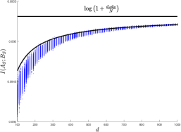
Figure 1. Mutual information scattering vs. $\log(1+\rho)$ for $d_{C}=1$ and $d_{A}=d_{B}=d$. In this experiment, we fixed the percentage of spurious tuples $\rho(R,\mathbf{S})$, and accordingly randomly generated $N\mathrel{\stackrel{{\scriptstyle\textsf{\tiny def}}}{{=}}}\frac{d_{A}d_{B}}{(1+\rho(R,\mathbf{S}))}$ tuples from the random relation model (Definition 5.2), and plotted the resulting mutual information. As can be seen, as the database grows, the mutual informatio approaches $\log(1+\rho)$.

Proposition 5.1 reduces the problem of upper bounding $\log[1+\rho(R,\mathbf{S})]$ to bounding each of the terms $\log[1+\rho(R,\phi_{i})]$ in (29), each of them corresponding to the relative number of spurious tuples of the $m-1$ MVDs in the support of ${\mathcal{T}}$. Considering an arbitrary MVD, which we henceforth denote for simplicity by $\phi\mathrel{\stackrel{{\scriptstyle\textsf{\tiny def}}}{{=}}}C\twoheadrightarrow A|B$, Lemma 4.1 implies the lower bound $\log[1+\rho(R,\phi_{i})]\geq I(A;B\mid C)$, since an MVD is a simple instance of an acyclic schema. However, obtaining an upper bound on $\log[1+\rho(R,\phi_{i})]$ in terms of $I(A;B\mid C)$ is challenging because the mutual information $I(A;B\mid C)$ varies wildly for an MVD $\phi$ even when $\rho(R,\phi)$ and the domains sizes $d_{A},d_{B}$ and $d_{C}$ remain constant (where $d_{A}\mathrel{\stackrel{{\scriptstyle\textsf{\tiny def}}}{{=}}}|{\Pi}_{A}(R)|$, and similarly for $d_{B}$ and $d_{C}$). Figure 1 illustrates this phenomenon in the simple case in which $d_{C}=1$ and so $C$ is a degenerated random variable, and $d_{A}=d_{B}$. In other words, the value $I(A;B\mid C)$ depends on the actual contents of the relation instance $R$. However, while $I(A;B\mid C)$ might not be an accurate upper bound to $\log[1+\rho(R,\phi)]$ for an arbitrary relation, it may hold that it is an approximate upper bound for most relations. Therefore, we next propose a random relation model, in which the tuples of the relation $R$ are chosen at random. We then establish an upper bound on $\log[1+\rho(R,\phi)]$ that holds with high probability over this randomly chosen relation.

Definition 5.2 (Random relation model).

Let $\Omega\mathrel{\stackrel{{\scriptstyle\textsf{\tiny def}}}{{=}}}\{X_{1},\ldots,X_{n}\}$ be a set of attributes with domains $\mathcal{D}(X_{1}),\dots,\mathcal{D}(X_{n})$, and assume w.l.o.g. that $\mathcal{D}(X_{i})\mathrel{\stackrel{{\scriptstyle\textsf{\tiny def}}}{{=}}}[d_{i}]$ for $\{d_{i}\}_{i=1}^{n}\subset\mathbb{N}_{+}$. Let $N\in\mathbb{N}_{+}$ be given such that $0<N\leq\prod_{i=1}^{n}d_{i}$. Let $S$ be a set of $N$ tuples chosen uniformly at random from $\bigtimes_{i=1}^{n}[d_{i}]$, without replacement. Given $S$, we let $P_{S}$ denote the empirical distribution over $S$:

(32) $$P_{S}\left[\bigcap_{i=1}^{n}\{X_{i}=\ell_{i}\}\right]=\begin{cases}\frac{1}{N},&(\ell_{1},\ell_{2},\ldots,\ell_{n})\in S\\ 0,&\text{otherwise}\end{cases}$$

for any $(\ell_{1},\ell_{2},\ldots,\ell_{n})\in\bigtimes_{i=1}^{n}[d_{i}]$.

In other words, in the random relational model $R$ is chosen uniformly at random from the set of possible relations of size $N$, that is, from the set ${\mathcal{R}}(\Omega)\cap\{R\colon|R|=N\}$. The next proposition states that the existence of a high probability bound on the relative number of spurious tuples associated with an arbitrary MVD $\phi$, implies the existence of a high-probability upper bound on the relative number of spurious tuples $\log[1+\rho(R,\mathbf{S})]$ associated with an acyclic schema $\mathbf{S}$.

Proposition 5.3.

Let $\epsilon(\phi,N,\delta)\geq 0$ where $\phi\mathrel{\stackrel{{\scriptstyle\textsf{\tiny def}}}{{=}}}C\twoheadrightarrow A|B$ is an MVD, $\delta\in(0,1)$, and $R$ is a random relation over attributes $ABC$, where $|R|=N$. Let $\mathbf{S}=\{\Omega_{1},\ldots,\Omega_{m}\}$ be an acyclic schema over the attributes of $R$ with join tree ${\mathcal{T}}$. If the random relation $R$ satisfies $\log[1+\rho(R,\phi)]\leq I(A;B\mid C)+\epsilon(\phi,N,\delta)$, with probability larger than $1-\frac{\delta}{m-1}$, for all MVDs $\phi_{i}\mathrel{\stackrel{{\scriptstyle\textsf{\tiny def}}}{{=}}}\Delta_{i}\twoheadrightarrow\Omega_{1\mathrel{\mathop{\ordinarycolon}}i-1}|\Omega_{i\mathrel{\mathop{\ordinarycolon}}m}$ in the support of    $\mathbf{S}$. Then:

(33) $$\log\left[1+\rho(R,\mathbf{S})\right] \leq\sum_{i=2}^{m}I(\Omega_{1\mathrel{\mathop{\ordinarycolon}}i-1};\Omega_{i\mathrel{\mathop{\ordinarycolon}}m}\mid\Delta_{i})+\epsilon_{i}$$

(34) $$\leq(m-1)\mathcal{J}({\mathcal{T}})+\sum_{i=2}^{m}\epsilon_{i}$$

with probability $1-\delta$, where $\epsilon_{i}\mathrel{\stackrel{{\scriptstyle\textsf{\tiny def}}}{{=}}}\epsilon\left(\Delta_{i}\twoheadrightarrow\Omega_{1\mathrel{\mathop{\ordinarycolon}}i-1}|\Omega_{i\mathrel{\mathop{\ordinarycolon}}m},N,\frac{\delta}{m-1}\right)$.

Proof.

For the MVD $\phi_{i}\mathrel{\stackrel{{\scriptstyle\textsf{\tiny def}}}{{=}}}\Delta_{i}\twoheadrightarrow\Omega_{1\mathrel{\mathop{\ordinarycolon}}i-1}|\Omega_{i\mathrel{\mathop{\ordinarycolon}}m}$, it holds that

(35) $$\log[1+\rho(R,\phi)]\leq I(\Omega_{1\mathrel{\mathop{\ordinarycolon}}i-1};\Omega_{i\mathrel{\mathop{\ordinarycolon}}m}\mid\Delta_{i})+\epsilon\left(\phi_{i},N,\frac{\delta}{m-1}\right)$$

with probability larger than $1-\frac{\delta}{m-1}$. Then, (33) follows from Proposition 5.1, and a union bound over the $m-1$ MVDs $\{\phi_{i}\}_{i=2}^{m}$ in the support of $\mathbf{S}$. The bound (34) follows from (8) in Theorem 2.3. ∎

Hence, the problem of deriving an upper bound on $\log[1+\rho(R,\mathbf{S})]$, which holds with high probability, is reduced to the problem of showing that $\log[1+\rho(R,\phi)]\leq I(A;B\mid C)+\epsilon(\phi,N,\delta)$ holds with high probability for an MVD $\phi\mathrel{\stackrel{{\scriptstyle\textsf{\tiny def}}}{{=}}}C\twoheadrightarrow A|B$, in the setting of the random relational model, assuming that the relation size is fixed to $N$. In other words, it now suffices to prove the probabilistic upper bound for a single MVD in the random relation model (Definition 5.2).

In what follows, we focus on a single MVD, denoted $\phi\mathrel{\stackrel{{\scriptstyle\textsf{\tiny def}}}{{=}}}C\twoheadrightarrow A|B$, and where $d_{A},d_{B}$ and $d_{C}$ are the domain sizes of $A$, $B$, and $C$, respectively. Then, for any $S\subseteq[d_{A}]\times[d_{B}]\times[d_{C}]$

(36) $$P_{S}\left[A=a,B=b,C=c\right]=\begin{cases}\frac{1}{N},&(a,b,c)\in S\\ 0,&\text{otherwise}\end{cases}$$

for any $(a,b,c)\in[d_{A}]\times[d_{B}]\times[d_{C}]$, and the relation is such that the set $S$ is chosen uniformly at random from $[d_{A}]\times[d_{B}]\times[d_{C}]$ from all possible sets of size $N$. While both the domain sizes $d_{A},d_{B}$ and $d_{C}$ and relation size $N$ are fixed in this model, the mutual information $I(A;B\mid C)$ is a random variable due to the random choice of the set $S$. Specifically, the random relation instance $S\subseteq[d_{A}]\times[d_{B}]\times[d_{C}]$ where $|S|=N$, is a random variable, and each specific realization $S=s$, defines a triplet of random variables $A_{s}\mathrel{\stackrel{{\scriptstyle\textsf{\tiny def}}}{{=}}}{\Pi}_{A}(s)$, $B_{s}\mathrel{\stackrel{{\scriptstyle\textsf{\tiny def}}}{{=}}}{\Pi}_{B}(s)$ and $C_{s}\mathrel{\stackrel{{\scriptstyle\textsf{\tiny def}}}{{=}}}{\Pi}_{C}(s)$. Consequently, every such set $s$ defines various information theoretic measures, such as $H(A_{s})$, $I(A_{s};B_{s}\mid C_{s})$, and so on. Furthermore, a random choice of $S$ makes these information measures random quantities themselves, for example, $H(A_{S})$ and $I(A_{S};B_{S}\mid C_{S})$ are random variables. In a similar fashion, if we let $R_{S}$ denote the random relation defined by $S$, then $\rho(R_{S},\phi)$ is again a random variable. Our main result regarding the mutual information of an MVD is as follows:

Theorem 5.1 (Confidence bound of the random mutual information of an MVD).

Let $\delta\in(0,1)$. Assume w.l.o.g. that $d_{A}\geq d_{B}$, denote $\overline{d}\mathrel{\stackrel{{\scriptstyle\textsf{\tiny def}}}{{=}}}\max\{d_{A},d_{C}\}$ and assume further that

(37) $$N\geq 256d_{A}\overline{d}\log\left(\frac{384\overline{d}}{\delta}\right).$$

Let

(38) $$\epsilon^{*}\left(\phi,N,\delta\right)\mathrel{\stackrel{{\scriptstyle\textsf{\tiny def}}}{{=}}}60\sqrt{\frac{d_{A}\overline{d}\log^{3}\left(\frac{6Nd_{C}}{\delta}\right)}{N}}$$

If $R_{S}$ is drawn from the random relation model of Definition 5.2, then

(39) $$\log\left[1+\rho(R_{S},\phi)\right]\leq I(A_{S};B_{S}\mid C_{S})+\epsilon^{*}\left(\phi,N,\delta\right)$$

with probability larger than $1-\delta$.

The proof of Theorem 5.1 is fairly complicated, and is discussed in detail in Section 5.1. Theorem 5.1 shows that, with high probability, the upper bound $\log\left[1+\rho(R_{S},\phi)\right]\leq I(A_{S};B_{S}\mid C_{S})$ approximately holds, up to an additive factor of $\tilde{O}(\sqrt{d_{A}\max\{d_{A},d_{C}\}/N})$, where the $\tilde{O}(\cdot)$ hides logarithmic terms. This result is suitable for large domain sizes, and when the number of tuples $N$ is proportional to the domain sizes. More accurately, the bound holds whenever $N=\tilde{\Omega}(d_{A}d_{C})$, where $\tilde{\Omega}(\cdot)$ hides logarithmic terms (condition (37)), which is a mild condition when targeting a low fraction of spurious tuples. So, when $\delta$ is fixed to some desired reliability, and the qualifying condition (37) holds, then the deviation term in the claim of Theorem 5.1 is given by $\epsilon^{*}(\phi,N,\delta)=\tilde{O}(\sqrt{\max\{d_{A}^{2},d_{A}d_{C})/N})$. Hence, when $N$ increases as $N=\tilde{\omega}(\max\{d_{A}^{2},d_{A}d_{C}\})$, then $\epsilon^{*}(\phi,N,\delta)$ vanishes. For example, if $d_{A}=d_{B}=d_{C}\equiv d$, then the deviation term is $\epsilon^{*}(\phi,N,\delta)=O(\sqrt{\frac{d^{2}\log^{3}(Nd)}{N}})$. and this deviation term vanishes if $N=\omega(d^{2}\log^{3}(Nd))$. As a more concrete example, if $N=\tfrac{1}{2}d^{3}$, then the deviation term is $\epsilon^{*}(\phi,N,\delta)=O(\sqrt{\frac{\log^{3}(d)}{d}})$ which vanishes at a rather fast rate with increasing $d$. Moreover, the dependency of the deviation term in $\delta$ is mild, and scales as $\log^{3/2}(1/\delta)$ which is close to a sub-exponential dependence.

5.1. Proof of Theorem 5.1: A Confidence Interval for the Mutual Information

In this section, we discuss in detail the proof of Theorem 5.1. We focus on the case in which $C$ is a degenerate random variable ($d_{C}=1$) since the main components of the proof are already present in this simple case. When $d_{C}=1$, the conditional mutual information is reduced to the standard mutual information $I(A_{S};B_{S})$. In turn, the random set $S$ which determines the random relation is chosen uniformly at random from all subsets of $[d_{A}]\times[d_{B}]$ of a given size. To avoid confusion with the non-degenerate model, we denote this size by $\eta$ (rather than by $N$) whenever $d_{C}=1$. The mutual information can then be decomposed as $I(A_{S};B_{S})=H(A_{S})+H(B_{S})-H(A_{S},B_{S})$ (Cover and Thomas, 2006, Section 2.4), and by the definition of the random model, $R_{S}=(A_{S},B_{S})$ is distributed uniformly over the possible sets of size $\eta$. Thus $H(A_{S},B_{S})=\log\eta$ with probability $1$ (over the choice of $S$), and $I(A_{S};B_{S})=H(A_{S})+H(B_{S})-\log\eta$. Due to symmetry, the analysis of $H(A_{S})$ and $H(B_{S})$ is analogous, and so we next focus on the former. The main ingredient of the proof of Theorem 5.1 is a confidence interval for the random entropy $H(A_{S})$, when $A_{S}$ is chosen from a random relation model similar to the one of Definition 5.2, albeit with a degenerated $C$, that is, $d_{C}=1$. At a later stage, we discuss the generalization of this reuslt to $d_{C}>1$. The confidence bound on $H(A_{S})$ is as follows:

Theorem 5.2.

Let $A_{S}$ be drawn according to the random relation model of Definition 5.2 with $d_{C}=1$ and $N=\eta$. Assume w.l.o.g. that $d_{A}\geq d_{B}$ and that

(40) $$\eta\geq 128d_{A}\log\left(\frac{128d_{A}}{\delta}\right).$$

Then, for any probability $\delta\in(0,1)$ it holds that

(41) $$\log d_{A}\geq H(A_{S})\geq\log d_{A}-20\sqrt{\tfrac{d_{A}\log^{3}\left(\frac{\eta}{\delta}\right)}{\eta}}$$

with probability $1-\delta$, over the random choice of the set $S$.

The proof of Theorem 5.2 comprises most of the proof of Theorem 5.1, and requires a diverse set of mathematical techniques, discussed in Section 5.2. For now, taking the result of Theorem 5.2 as given, a high probability bound on the value of $I(A_{S};B_{S})$ for the random relation model with degenerated $C$ can be obtained as a simple corollary to Theorem 5.2, as follows:

Corollary 5.3.0.

Let $\overline{\rho}=\frac{d_{A}\cdot d_{B}}{\eta}-1$. Then, under the same assumptions of Theorem 5.2,

(42) $$I(A_{S};B_{S})\geq\log\left(1+\overline{\rho}\right)-40\sqrt{\tfrac{d_{A}\log^{3}\left(\frac{2\eta}{\delta}\right)}{\eta}},$$

with probability $1-\delta$, over the random choice of the set $S$.

Corollary 5.3 will be used in the proof of Theorem 5.1. Beyond that, it also reveals the tightness of the mutual information bound in the simpler setting of a degenerated MVD $(d_{C}=1)$. Indeed, since $A_{S}\subseteq[d_{A}]$ and $B_{S}\subseteq[d_{B}]$ for all realizations of $S$, then $\rho(R_{S},\phi)\leq\frac{d_{A}d_{B}}{\eta}-1=\overline{\rho}$. Thus, Corollary 5.3 implies

(43) $$I(A_{S};B_{S})\geq\log\left[1+\rho(R_{S},\phi)\right]-40\sqrt{\tfrac{d_{A}\log^{3}\left(\frac{2\eta}{\delta}\right)}{\eta}},$$

but actually shows the stronger bound (42).

Proof outline of Theorem 5.1

At this point, let us take the results of Theorem 5.2 and Corollary 5.3 as granted. Then, the proof of Theorem 5.1 is essentially a generalization of the result of Theorem 5.2 to the case in which $d_{C}>1$. Let us define $R_{\ell}\mathrel{\stackrel{{\scriptstyle\textsf{\tiny def}}}{{=}}}\sigma_{C=\ell}(R)$. Then, in the random relation model $N_{S}(\ell)=|R_{\ell}|$ is a random variable, and beyond the randomness in the joint distribution of $(A_{S},B_{S})$ when conditioned on any $C=\ell$, there is also randomness in the number of tuples in the random relation, whenever $C=\ell$. Hence, the mutual information conditioned on the specific value of $C=\ell$, to wit, $I(A_{S};B_{S}\mid C_{S}=\ell)$, is drawn from the random model in Definition 5.2 with $N$ being replaced by $N_{S}(\ell)$ (the latter being a random variable due to the random choice of $S$). The result of Corollary 5.3, regarding the mutual information of a pair of random variables $A_{S},B_{S}$, can then be used conditionally on $C_{S}=\ell$, where $\eta$ is being replaced by $N_{S}(\ell)$. In order for this result to hold, the qualifying condition of Corollary 5.3, to wit $N_{S}(\ell)\geq 128d_{A}\log(\frac{128d_{A}}{\delta})$, should hold for all $\ell\in[d_{C}]$. The proof begins by showing that this condition indeed holds for all $\ell\in[d_{C}]$ with high probability. This is proved in Lemma C.1 in Appendix C, and is based on the fact that $N_{S}(\ell)$ is a hypergeometric random variable, and on a concentration result by Serfling (Serfling, 1974) for such random variables. The proof then assumes that all the following holds: (I) For all $\ell\in[d_{C}]$, $N_{S}(\ell)$ is sufficiently large so that the qualifying condition of Corollary 5.3 holds. (II) For each $\ell\in[d_{C}]$, the confidence bound in Corollary 5.3 holds. (III) $H(C_{S})$ is close to $\log d_{C}$.

Specifically, Lemma C.1 assures that the first condition holds with high probability; Corollary 5.3 assures that the second condition holds with high probability; a simple modification of Theorem 5.2 shows that the third condition holds with high probability. By the union bound, the event in which the set $s\subseteq[d_{A}]\times[d_{B}]\times[d_{C}]$ simultaneously satisfies properties (I), (II) and (III) has high probability. The proof is completed by considering a set $s\subseteq[d_{A}]\times[d_{B}]\times[d_{C}]$, which satisfies properties (I), (II) and (III), and relating $\log[1+\rho(R_{s},\phi)]$ to the mutual information. Concretely, an application of the log sum inequality (Lemma D.8 in Appendix D), shows that (see (335))

(44) $$\log\left[1+\rho(R_{s},\phi)\right]\leq\log d_{C}-H(C_{s})\\ +\sum_{\ell\in[d_{C}]}\mathsf{P}[C_{s}=\ell]\log\left[1+\overline{\rho}_{s}(\ell)\right],$$

which can be bounded by conditional mutual information, and an additional additive deviation term, utilizing the aforementioned assumption that $s$ satisfies properties (I), (II) and (III).

5.2. Confidence Bound of the Conditional Entropy

In this section, we describe the proof of the confidence interval in Theorem 5.2, which is comprised of three main steps on its own: (I) A bound on the expected value of $H(A_{S})$, which is shown to be asymptotically close to $\log d_{A}$ under the random relation model. (II) A concentration result of $H(A_{S})$ to its expected value. (III) A combination of these bounds. In the next two subsections we provide a formal statement of the first two steps, and outline their proof. The full proof is deferred to Appendix B, along with the third part (which is more technical in its nature) and completes the proof of Theorem 5.2.

5.2.1. The expected value of the entropy

In this section, we state a bound on the average mutual information ${\tt\mathbb{E}}[H(A_{S})]$ and outline its proof. Let us denote, for notational brevity,

(45) $$C(d)\mathrel{\stackrel{{\scriptstyle\textsf{\tiny def}}}{{=}}}\frac{2\log(d)}{\sqrt{d}}.$$

Proposition 5.4 (Bounds on the expected entropy).

Assume that $d_{A}\geq d_{B}$ and that $\eta\geq 60d_{A}$. If $S$ is chosen uniformly at random from one of the possible subsets of $[d_{A}]\times[d_{B}]$ of size $\eta$ then

(46) $$0\leq\log d_{A}-{\tt\mathbb{E}}[H(A_{S})]\leq C(d_{B}),$$

where $C(d)$ is as defined in (45). An analogous result hold for $H(B_{S})$:

(47) $$0\leq\log d_{B}-{\tt\mathbb{E}}[H(B_{S})]\leq C(d_{A}).$$

We next present the main ideas of the proof of Proposition 5.4. As a first step, we identify that the expected value ${\tt\mathbb{E}}[H(A_{S})]$ is, in fact, a conditional entropy $H(A\mid S)$, to wit,

(48) $${\tt\mathbb{E}}\left[H(A_{S})\right]=\sum_{s}\mathsf{P}[S=s]\cdot H(A_{s})=H(A\mid S).$$

The crux of the proof of Proposition 5.4 requires lower bounding $H(A\mid S)$. Nonetheless, to illuminate the challenge in the proof, it is insightful to first note that as conditioning reduces entropy (Cover and Thomas, 2006, Theorem 2.6.5), and so

(49) $$H(A\mid S)\leq H(A).$$

Using the symmetry of the distribution of the set $S$, it follows that $H(A)=\log d_{A}$ (see Lemma B.1 in Appendix B for a rigorous proof) . So, Proposition 5.4 states that $H(A\mid S)$ is close to its unconditional value $H(A)$, up to $C(d_{B})$. In other words, we need to show that the conditioning (over the random variable $S$) only slightly reduces entropy in (49).

To further delve into the proof of this property, we closely inspect $H(A\mid S)$. For any $(i,j)\in[d_{A}]\times[d_{B}]$, we define the random variable $U_{S}(i,j)\mathrel{\stackrel{{\scriptstyle\textsf{\tiny def}}}{{=}}}\boldsymbol{\mathds{I}}\{(i,j)\in S\}\}$, which indicates if the tuple $(i,j)$ is in the random relation $R_{S}$ (see Definition 5.2). By symmetry, $\mathsf{P}(U_{S}(i,j)=1)=\frac{\eta}{d_{A}d_{B}}$ for all $(i,j)\in[d_{A}]\times[d_{B}]$, and hence $\{U_{S}(i,j)\}_{(i,j)\in[d_{A}]\times[d_{B}]}$ are identically distributed. The values $\{U_{S}(i,j)\}_{(i,j)\in[d_{A}]\times[d_{B}]}$ uniquely determine $R_{S}$, and so also the entropy $H(A_{S})$. However, $\{U_{S}(i,j)\}_{(i,j)\in[d_{A}]\times[d_{B}]}$ are dependent random variables, and such random variables are typically more difficult to handle than independent ones. Letting $Y_{S}\equiv Y_{S}(1)\mathrel{\stackrel{{\scriptstyle\textsf{\tiny def}}}{{=}}}\frac{1}{d_{B}}\sum_{j\in[d_{B}]}U_{S}(1,j)$, it can be shown that (see (112) in Appendix B)

(50) $$H(A\mid S) =-\frac{d_{A}d_{B}}{\eta}{\tt\mathbb{E}}\left[Y_{S}\cdot\log(Y_{S})\right]+\log\frac{\eta}{d_{B}}.$$

Noting that $f(t)\mathrel{\stackrel{{\scriptstyle\textsf{\tiny def}}}{{=}}}t\log(t)$ is a convex function on $\mathbb{R}_{+}$, one obtains from Jensen’s inequality that

(51) $$-{\tt\mathbb{E}}\left[Y_{S}\cdot\log(Y_{S})\right]\leq-{\tt\mathbb{E}}[Y_{S}]\log{\tt\mathbb{E}}[Y_{S}],$$

and since ${\tt\mathbb{E}}(Y_{S})=\frac{\eta}{d_{A}d_{B}}$, it immediately follows that

(52) $$H(A\mid S)\leq\log d_{A}=H(A),$$

as is already known from the conditioning reduces entropy property (49). From the above discussion, we deduce that in order to obtain a lower bound on $H(A\mid S)$, which is close to $H(A)=\log d_{A}$, it is required to show that the Jensen-based bound in (51) is close to an equality. Trivially, if $Y_{S}$ had been a deterministic quantity, then any Jensen-based inequality is satisfied with equality, and specifically (51). Continuing this line of thought, one expects that if $Y_{S}$ is tightly concentrated around its expected value (i.e., “close” to being deterministic), then (51) approximately holds with equality. Indeed, such relations have been extensively explored via the functional entropy of a non-negative random variable $X$, defined as

(53) $$\operatorname{\mathrm{Ent}}(X)\mathrel{\stackrel{{\scriptstyle\textsf{\tiny def}}}{{=}}}{\tt\mathbb{E}}\left[X\log X\right]-{\tt\mathbb{E}}[X]\log\left[{\tt\mathbb{E}}(X)\right].$$

The functional entropy is non-negative, and is conveniently upper bounded via logarithmic Sobolev inequalities (LSIs) (Boucheron et al., 2013, Chapter 5). Specifically, these inequalities bound $\operatorname{\mathrm{Ent}}(X)$ by the Efron-Stein variance of $X$ (Boucheron et al., 2013, Chapter 5), which in turn quantifies the concentration of $Y$ around its expected value – low Efron-Stein variance implies tight concentration around the expected value, and thus low functional entropy by LSIs. Therefore, the proof addresses the bounding of $\operatorname{\mathrm{Ent}}(Y_{S})$. Nonetheless, LSIs are typically derived for functions of independent random variables, whereas here, as discussed, $Y_{S}\mathrel{\stackrel{{\scriptstyle\textsf{\tiny def}}}{{=}}}\frac{1}{d_{B}}\sum_{j\in[d_{B}]}U_{S}(1,j)$ is an average of dependent random variables. To address this matter, we define a new set of random variables $\{V(j)\}_{j\in[d_{B}]}$, so that each $V(j)$ has the same marginal distribution as $U_{S}(1,j)$, but where the $\{V(j)\}_{j\in[d_{B}]}$ are independent. In other words, $\{V(j)\}{}_{j\in[d_{B}]}$ is a set of Bernoulli random variables for which $\mathsf{P}[V(j)=1]=\frac{\eta}{d_{A}d_{B}}$, thus possibly asymmetric. We then define $\tilde{Y}\mathrel{\stackrel{{\scriptstyle\textsf{\tiny def}}}{{=}}}\frac{1}{d_{B}}\sum_{j\in[d_{B}]}V(j)$, and instead of directly bounding $\operatorname{\mathrm{Ent}}(Y_{S})$ as is required for the proof, we bound $\operatorname{\mathrm{Ent}}(\tilde{Y})$ and the difference between the two functional entropies, to wit, we write

(54) $$\operatorname{\mathrm{Ent}}(Y_{S})=\operatorname{\mathrm{Ent}}(\tilde{Y})+[\operatorname{\mathrm{Ent}}(Y_{S})-\operatorname{\mathrm{Ent}}(\tilde{Y})],$$

and then separately bound each of the terms. Denoting $\bar{\rho}\mathrel{\stackrel{{\scriptstyle\textsf{\tiny def}}}{{=}}}\frac{d_{A}d_{B}}{\eta}-1$ (which is an upper bound on the relative number of spurious tuples), we show in Lemma B.2 in Appendix B that

(55) $$\operatorname{\mathrm{Ent}}(\tilde{Y})\leq\frac{2\overline{\rho}\log(1/\overline{\rho})}{1-\overline{\rho}}\cdot\frac{1}{d_{B}}.$$

The proof of Lemma B.2 is based on a LSI for the asymmetric Bernoulli random variables $\{V(j)\}_{j\in[d_{B}]}$ (Boucheron et al., 2013, Chapter 5), along with a careful bounding of the Efron-Stein variance of $\tilde{Y}$. The next term in the decomposition of $\operatorname{\mathrm{Ent}}(Y_{S})$ in (54) is absolutely bounded in Lemma B.3 in Appendix B as

(56) $$\left|\operatorname{\mathrm{Ent}}(Y_{S})-\operatorname{\mathrm{Ent}}(\tilde{Y})\right|\leq\sqrt{\frac{2\log^{2}(d_{B})}{d_{B}}}.$$

Summing the bounds on $\operatorname{\mathrm{Ent}}(\tilde{Y})$ and $|\operatorname{\mathrm{Ent}}(Y_{S})-\operatorname{\mathrm{Ent}}(\tilde{Y})|$ leads to a bound on $\operatorname{\mathrm{Ent}}(Y_{S})$, which in turn shows that the Jensen-bound in (51) is close to equality. This shows that $H(A\mid S)\leq\log d_{A}$ in fact approximately achieved, up to the defined vanishing term $C(d_{B})$.

5.2.2. The concentration to the expected value of the entropy

We next discuss the second step of the proof of Theorem 5.2. We state a concentration bound on $H(A_{S})$ to ${\tt\mathbb{E}}[H(A_{S})]$ and outline its proof. For brevity, for $t\in\mathbb{R}_{+}$, we denote

(57) $$h(t)\mathrel{\stackrel{{\scriptstyle\textsf{\tiny def}}}{{=}}}t\log(1+t).$$

Proposition 5.5.

Assume that $d_{A}>d_{B}$, that $\eta\geq 60d_{A}$ and that $\eta\leq d_{A}d_{B}-d_{B}$. Then, it holds that

(58) $$\mathsf{P}\left[\left|H(A_{S})-{\tt\mathbb{E}}[H(A_{S})]\right|>t\right]\\ \leq\frac{1}{2}\cdot e^{-\frac{\eta}{12}}+\frac{1}{2}\exp\left\{-\frac{\eta}{2d_{A}}\cdot h\left(\frac{r}{2\log(\eta/e)}\right)+4\log(\eta)\right\},$$

where

(59) $$r=\max\left\{0,t-\frac{8d_{A}}{\eta}-C(d_{B})\right\}.$$

Previously, in Section 5.2.1, we defined the random variables $\{U_{S}(i,j)\}_{i\in[d_{A}],j\in[d_{B}]}$ and then $\{Y_{S}(i)\}_{i\in[d_{A}]}$. For the proof of Proposition 5.5 it will be more convenient to use their scaled version

(60) $$Z_{S}(i)\mathrel{\stackrel{{\scriptstyle\textsf{\tiny def}}}{{=}}}d_{B}\cdot Y_{S}(i)=\sum_{j\in[d_{B}]}U_{S}(i,j).$$

By the definition of the random relation model, for each $i\in[d_{A}]$, $Z_{S}(i)\sim\text{Hypergeometric}(d_{A}d_{B},d_{B},\eta)$, that is, a hypergeometric random variable, with population size $d_{A}d_{B}$, $d_{B}$ success states in the population, and $\eta$ draws. We also note that since ${\tt\mathbb{E}}[Y_{S}(i)]=\frac{\eta}{d_{A}d_{B}}$ then ${\tt\mathbb{E}}[Z_{S}(i)]=\frac{\eta}{d_{A}}$. Since $\{Z_{S}(i)\}_{i\in[d_{A}]}$ are dependent random variables, the first step of the proof uses a union bound over all $i\in[d_{A}]$, and thus reduces the probability required to be bounded to just a single one of them, say $Z_{S}(1)$. Specifically, the first step of the proof (see (208) in Appendix B) shows that

(61) $$\mathsf{P}\left[\left|H(A_{S})-{\tt\mathbb{E}}[H(A_{S})]\right|>t\right]\\ \leq d_{A}\cdot\mathsf{P}\left[\left|g\left(\frac{Z_{S}}{\eta}\right)-\frac{{\tt\mathbb{E}}[H(A_{S})]}{d_{A}}\right|>\frac{t}{d_{A}}\right],$$

where $Z_{S}\equiv Z_{S}(1)$, and $g(t)\mathrel{\stackrel{{\scriptstyle\textsf{\tiny def}}}{{=}}}-t\log t$. Thus, the probability that the entropy is close to its expected value is bounded by the probability that a function of a hypergeometric random variable is close to its expectation. To bound the latter probability, we aim to use known concentration results, and specifically, concentration of Lipschitz functions of Poisson random variables. Therefore, the next step is to replace the hypergeometric random variable $Z_{S}$ with a Poisson random variable $W\sim\text{Poisson}$($\frac{\eta}{d_{A}}$), which has the same mean ${\tt\mathbb{E}}[W]=\frac{\eta}{d_{A}}={\tt\mathbb{E}}[Z_{S}]$. As is well known, the binomial distribution (and more generally, the multinomial distribution) can be “Poissonized” in the sense that the probability of any event under the binomial distribution is upper bounded by the same probability under the Poisson distribution, with a proper factor (Mitzenmacher and Upfal, 2017, Thm. 5.7). The hypergeometric is known to behave similarly to the binomial distribution, ,and so one may expect that it can also be “Poissonized”. Lemma B.4 in Appendix B, which is a preliminary step to the proof of Proposition 5.5, shows this Poissonization effect, and states the proper condition and constants. Its statement and results are general, and may be of independent interest. Equipped with the “Poissonization bound”, $Z_{S}$ can be replaced by $W$, and as a result, the bound in (61) is further upper bounded with a similar bound, except that the hypergeometric random variable $Z_{S}$ is replaced with a Poisson random variable $W$, and a larger multiplicative pre-factor ($21d_{A}^{3}$ instead of just $d_{A}$) The next matter to address is that $g(t)=-t\log t$ is not a Lipschitz function since its derivative is unbounded for $t\downarrow 0$ as well as $t\uparrow\infty$ (note that while $Z_{S}\leq d_{B}$ with probability $1$, $W$ is unbounded). We first address the $t\downarrow 0$ case. Since $W$ is supported on integers, the minimal non-zero argument possible for $g(\frac{W}{\eta})$ is $1/\eta$. So, if we restrict $t\in[\frac{1}{\eta},1]$ then $g(t)$ is a Lipschitz function with semi-norm $\frac{1}{\eta}\log\eta$. Based on this observation we propose a function $\hat{g}_{\eta}(t)$ which well approximates $g(t)$ on one hand, and is Lipschitz on the other hand. By an application of the triangle inequality, the term in (61) is upper bounded as

(62) $$\left|g\left(\frac{W}{\eta}\right)-\frac{{\tt\mathbb{E}}[H(A_{S})]}{d_{A}}\right|\leq\left|g\left(\frac{W}{\eta}\right)-\hat{g}_{\eta}\left(\frac{W}{\eta}\right)\right|+\\ \left|\hat{g}_{\eta}\left(\frac{W}{\eta}\right)-{\tt\mathbb{E}}\left[\hat{g}_{\eta}\left(\frac{W}{\eta}\right)\right]\right|+\left|{\tt\mathbb{E}}\left[\hat{g}_{\eta}\left(\frac{W}{\eta}\right)\right]-\frac{{\tt\mathbb{E}}[H(A_{S})]}{d_{A}}\right|.$$

The first term in (62) is bounded as $1/\eta$ with probability $1$ directly from the construction of the function $\hat{g}_{\eta}(t)$. The last term in (62) is bounded in Lemma B.5, whose proof is rather technical, and utilizes both the bound on the expected value of Proposition 5.4 previously stated, as well as tools such as Poisson LSI (see Lemma D.5 in Appendix D). The proof continues by bounding the probability that the middle term in (62) is larger than some value. The main tool for this bound in a concentration bound for Lipschitz functions of Poisson random variables. This bound is not used directly, since $\hat{g}_{\eta}(t)$ is not Lipschitz over the entire real line. However, the argument $W/\eta$ is small enough with high probability, and thus belong to the Lipschitz continuous part of this function. Additional approximation arguments show that this suffices to obtain tight upper bound. The combination of the bounds for all three terms then establishes the proof of Theorem 5.2.

6. Conclusion

We show that the KL-Divergence is a useful measure for capturing the loss of an AJD with respect to the number of redundant tuples generated by the acyclic join. Our proposed random database model has allowed us to establish a high probability upper-bound on the percentage of redundant tuples, which coincides with the deterministic lower bound for large databases. Overall, our findings provide insights into the information-theoretic nature of AJD loss.

APPENDIX

A. Proofs for Section 3

Proposition 3.1. Let $P(X_{1},\dots,X_{n})$ be any joint probability distribution over $n$ variables, and let $({\mathcal{T}},\chi)$ be a join tree where $\chi({\mathcal{T}})=\mathord{\{X_{1},\dots,X_{n}\}}$. Then $P\models{\mathcal{T}}$ (Definition 2.4) if and only if $P=P_{\mathcal{T}}$ where:

(63) $$P_{\mathcal{T}}(x_{1},\dots,x_{n})\mathrel{\stackrel{{\scriptstyle\textsf{\tiny def}}}{{=}}}\frac{\prod_{i=1}^{m}P[\Omega_{i}](\boldsymbol{\textbf{x}}[\Omega_{i}])}{\prod_{i=1}^{m-1}P[\Delta_{i}](\boldsymbol{\textbf{x}}[\Delta_{i}])}$$

where $P[\Omega_{i}]$ ($P[\Delta_{i}]$) denote the marginal probabilities over $\Omega_{i}$ ($\Delta_{i}$).

Proof.

We prove both directions by induction on $m=|\texttt{nodes}({\mathcal{T}})|$. If direction: we assume that $P\models{\mathcal{T}}$ (see Definition 2.4). When $m=1$ the claim is immediate, so assume that it holds for $m\geq 1$, and we prove for $|\texttt{nodes}({\mathcal{T}})|=m+1$. So $({\mathcal{T}},\chi)$ is a junction tree over $m+1$ nodes. Let $u_{m+1}$ denote a leaf in ${\mathcal{T}}$ where $\chi(u_{m+1})=\Omega_{m+1}$, and let $u_{p}=\texttt{parent}(u_{m+1})$ in ${\mathcal{T}}$ where $\chi(u_{p})=\Omega_{p}$. We let $\Delta_{m}=\Omega_{p}\cap\Omega_{m+1}$. By the assumption that $P\models{\mathcal{T}}$, then by Definition 2.4, we have that $I(\Omega_{(1\mathrel{\mathop{\ordinarycolon}}m)};\Omega_{m+1}|\Delta_{m})$. Now, create a new junction tree ${\mathcal{T}}^{\prime}$ where nodes $\Omega_{m+1}$ and $\Omega_{p}$ are combined to a single node $u_{x}$ where $\chi(u_{x})=\Omega_{m+1}\cup\Omega_{p}$. Since ${\mathcal{T}}$ is a junction tree (Definition 2.1), then so is ${\mathcal{T}}^{\prime}$. The set of edges of ${\mathcal{T}}^{\prime}$ is a subset of those of ${\mathcal{T}}$. Therefore, since $P\models{\mathcal{T}}$ then it must hold that $P\models{\mathcal{T}}^{\prime}$. Since $|\texttt{nodes}({\mathcal{T}}^{\prime})|=m$, then by the induction hypothesis we have that:

(64) $$P_{{\mathcal{T}}^{\prime}}(x_{1},\dots,x_{n})=\left(\frac{\prod_{i\in[m]\setminus\mathord{\{p\}}}P[\Omega_{i}](\textbf{x}[\Omega_{i}])}{\prod_{i\in[m-1]}P[\Delta_{i}](\textbf{x}[\Delta_{i}])}\right)\times P[\chi(u_{x})](\textbf{x}[\chi(u_{x})])$$

Since $I(\Omega_{(1\mathrel{\mathop{\ordinarycolon}}m)};\Omega_{m+1}|\Delta_{m})=0$, and since $\Omega_{p}\subseteq\Omega_{(1\mathrel{\mathop{\ordinarycolon}}m)}$ then $I(\Omega_{p};\Omega_{m+1}|\Delta_{m})=0$. Therefore, $P[\chi(u_{x})]=\frac{P[\Omega_{m+1}]P[\Omega_{p})]}{P[\Delta_{m}]}$. Substituting this back in (64) proves the claim for the junction tree ${\mathcal{T}}$ with $m+1$ nodes.

For the other direction, we assume that (63) holds, and prove by induction on $m=|\texttt{nodes}({\mathcal{T}})|$ that $P\models{\mathcal{T}}$. That is, we prove that for every edge $i\in\texttt{edges}({\mathcal{T}})$ where $i\in[m-1]$, it holds that $I(\Omega_{1,(i-1)};\Omega_{i}|\Delta_{i\mathrel{\mathop{\ordinarycolon}}m})=0$. The claim clearly holds for $m=1$ (since $\texttt{edges}({\mathcal{T}})=\emptyset$). We assume the claim holds for junction trees with at most $m\geq 1$ nodes, and prove for a junction tree ${\mathcal{T}}$ with $m+1$ nodes. Let $u_{m+1}$ be a leaf node in ${\mathcal{T}}$ with parent $u_{p}$. Let ${\mathcal{T}}^{\prime}$ be the junction tree that results from ${\mathcal{T}}$ by removing the node $u_{m+1}$. By the induction hypothesis we have that $I(\Omega_{1\mathrel{\mathop{\ordinarycolon}}(i-1)};\Omega_{i\mathrel{\mathop{\ordinarycolon}}m}|\Delta_{i})$ for every $i\in[1,m-1]$. Now, by the assumption of the claim, we have that $P_{\mathcal{T}}=P_{{\mathcal{T}}^{\prime}}\cdot\frac{P(\Omega_{m+1})}{P(\Delta_{m})}$. Since $\chi({\mathcal{T}}^{\prime})=\Omega_{(1\mathrel{\mathop{\ordinarycolon}}m)}$, we immediately get that $I(\Omega_{1\mathrel{\mathop{\ordinarycolon}}m};\Omega_{m+1}|\Delta_{m})=0$ as required. ∎

Lemma 3.3. Let $P(X_{1},\dots,X_{n})$ be a joint probability distribution over $n$ random variables, and let ${\mathcal{T}}$ be a join tree over $X_{1},\dots,X_{n}$ with bags $\Omega_{1},\dots,\Omega_{m}$. Then $P[\Omega_{i}]=P_{\mathcal{T}}[\Omega_{i}]$ for every $i\in[1,m]$, and $P[\Delta_{i}]=P_{\mathcal{T}}[\Delta_{i}]$ for every $i\in[1,m-1]$.

Proof.

We prove the claim by by induction on $m=|\texttt{nodes}({\mathcal{T}})|$. By definition of $P_{\mathcal{T}}$, the claim is immediate for $m=1$. So, we assume the claim holds for $m\geq 1$, and prove for $|\texttt{nodes}({\mathcal{T}})|=m+1$. Let $u_{m+1}$ be a leaf node in ${\mathcal{T}}$ where $\texttt{parent}(u_{m+1})=u_{p}$, and $\Omega_{m+1}\cap\Omega_{p}=\Delta_{m}$. Consider the tree $T^{\prime}$ where $\texttt{nodes}({\mathcal{T}}^{\prime})\mathrel{\stackrel{{\scriptstyle\textsf{\tiny def}}}{{=}}}\texttt{nodes}({\mathcal{T}})\setminus\mathord{\{u_{m+1}\}}$. Let $B_{m+1}\mathrel{\stackrel{{\scriptstyle\textsf{\tiny def}}}{{=}}}\Omega_{m+1}\setminus\Delta_{m}$. By the junction tree property (see Definition 2.1), $B_{m+1}\cap\Omega_{(1\mathrel{\mathop{\ordinarycolon}}m)}=\emptyset$. Accordingly, define $P_{{\mathcal{T}}^{\prime}}(\Omega\setminus B_{m+1})=\frac{\prod_{i=1}^{m}P[\Omega_{i}]}{\prod_{i=1}^{m-1}P[\Delta_{i}]}$. Since ${\mathcal{T}}^{\prime}$ has exactly $m$ nodes, and since $u_{p}\in\texttt{nodes}({\mathcal{T}}^{\prime})$, then by the induction hypothesis, it holds that $P[\Omega_{p}]=P_{{\mathcal{T}}^{\prime}}[\Omega_{p}]=\sum_{X\notin\Omega_{p}}P_{{\mathcal{T}}^{\prime}}(\Omega)$. Now,

(65) $$\sum_{X\notin\Omega_{m+1}}P_{\mathcal{T}}(\Omega) =\sum_{X\notin\Omega_{m+1}}\frac{\prod_{i=1}^{m}P[\Omega_{i}]}{\prod_{i=1}^{m-1}P[\Delta_{i}]}\cdot\frac{P[\Omega_{m+1}]}{P[\Delta_{m}]}$$

(66) $$=\frac{P[\Omega_{m+1}]}{P[\Delta_{m}]}\cdot\sum_{X\notin\Delta_{m}}\frac{\prod_{i=1}^{m}P[\Omega_{i}]}{\prod_{i=1}^{m-1}P[\Delta_{i}]}$$

(67) $$=\frac{P[\Omega_{m+1}]}{P[\Delta_{m}]}\cdot\sum_{X\notin\Delta_{m}}P_{{\mathcal{T}}^{\prime}}(\Omega\setminus B_{m+1})$$

(68) $$\overset{{\scriptstyle(a)}}{=}\frac{P[\Omega_{m+1}]}{P[\Delta_{m}]}\cdot\sum_{X\notin\Delta_{m}}\left(\sum_{X\notin\Omega_{p}}P_{{\mathcal{T}}^{\prime}}(\Omega\setminus B_{m+1})\right)$$

(69) $$\overset{{\scriptstyle(b)}}{=}\frac{P[\Omega_{m+1}]}{P[\Delta_{m}]}\cdot\sum_{X\notin\Delta_{m}}P[\Omega_{p}]$$

(70) $$\overset{{\scriptstyle(c)}}{=}\frac{P[\Omega_{m+1}]}{P[\Delta_{m}]}\cdot P[\Delta_{m}]=P[\Omega_{m+1}],$$

where $(a)$ follows since $\Delta_{m}\subseteq\Omega_{p}$, $(b)$ follows from the induction hypothesis, and $(c)$ follows again from $\Delta_{m}\subseteq\Omega_{p}$. ∎

Lemma 3.4.. The following holds for any joint probability distribution $P(X_{1},\dots,X_{n})$, and any join tree ${\mathcal{T}}$ over variables $X_{1},\dots,X_{n}$:

(71) $$\operatorname*{arg\,min}_{Q\models{\mathcal{T}}}D_{KL}(P||Q)=P_{{\mathcal{T}}}$$

Proof.

From Lemma 3.3 we have that, for every $i\in\mathord{\{1,\dots,m\}}$, $P_{\mathcal{T}}[\Omega_{i}]=P[\Omega_{i}]$ where, $\Omega_{i}=\chi(u_{i})$. Since $\Delta_{i}\subset\Omega_{i}$, then $P_{\mathcal{T}}[\Delta_{i}]=P[\Delta_{i}]$.

(72) $$\min_{Q\models{\mathcal{T}}}D_{KL}(P||Q) =\min_{Q\models{\mathcal{T}}}\mathbb{E}_{P}\left[\log\frac{P(X_{1},\dots,X_{n})}{Q(X_{1},\dots,X_{n})}\right]$$

(73) $$=\min_{Q\models{\mathcal{T}}}\mathbb{E}_{P}\left[\log\frac{P(X_{1},\dots,X_{n})}{P_{\mathcal{T}}(X_{1},\dots,X_{n})}\cdot\frac{P_{\mathcal{T}}(X_{1},\dots,X_{n})}{Q(X_{1},\dots,X_{n})}\right]$$

(74) $$=D_{KL}(P||P_{\mathcal{T}})+\min_{Q\models{\mathcal{T}}}\mathbb{E}_{P}\left[\log\frac{P_{\mathcal{T}}(X_{1},\dots,X_{n})}{Q(X_{1},\dots,X_{n})}\right]$$

Since the chosen distribution $Q(\textbf{X})$ has no consequence on the first term $D_{KL}(P||P_{\mathcal{T}})$, we take a closer look at the second term, to wit, $\min_{Q\models{\mathcal{T}}}\mathbb{E}_{P}\left[\log\frac{P_{\mathcal{T}}(X_{1},\dots,X_{n})}{Q(X_{1},\dots,X_{n})}\right]$. Since $Q\models{\mathcal{T}}$, then $Q(X_{1},\dots,X_{n})=\frac{\prod_{i=1}^{m}Q[\Omega_{i}](\textbf{X}[\Omega_{i}])}{\prod_{i=1}^{m-1}Q[\Delta_{i}](\textbf{X}[\Delta_{i}])}$ (see (10)). Hence, in what follows, we refer to $Q$ as $Q_{{\mathcal{T}}}$. In the remainder of the proof we show that:

(75) $$\mathbb{E}_{P}\left[\log\frac{P_{\mathcal{T}}(X_{1},\dots,X_{n})}{Q^{\mathcal{T}}(X_{1},\dots,X_{n})}\right] =\mathbb{E}_{P_{{\mathcal{T}}}}\left[\log\frac{P_{\mathcal{T}}(X_{1},\dots,X_{n})}{Q_{\mathcal{T}}(X_{1},\dots,X_{n})}\right]$$

(76) $$=D_{KL}(P_{\mathcal{T}}||Q_{\mathcal{T}}),$$

where the last equality follows from (5). Since $D_{KL}(P_{\mathcal{T}}||Q_{\mathcal{T}})\geq 0$, with equality if and only if $P_{\mathcal{T}}=Q_{\mathcal{T}}$, then choosing $Q_{\mathcal{T}}$ to be $P_{\mathcal{T}}$ minimizes $D_{KL}(P||Q)$, thus proving the claim. The remainder of the proof follows from the fact that $P[\Omega_{i}]=P_{\mathcal{T}}[\Omega_{i}]$ for every $i\in[1,m]$, and $P[\Delta_{j}]=P_{\mathcal{T}}[\Delta_{j}]$ for every $j\in[m-1]$.

$$\mathbb{E}_{P}\left[\log\frac{P_{\mathcal{T}}(X_{1},\dots,X_{n})}{Q^{\mathcal{T}}(X_{1},\dots,X_{n})}\right]$$

(77) $$=\sum_{\textbf{x}\in\mathcal{D}(\textbf{X})}P(\textbf{x})\log\frac{\prod_{i=1}^{m}P^{\mathcal{T}}[\Omega_{i}](\textbf{x}[\Omega_{i}])}{\prod_{i=1}^{m}Q^{\mathcal{T}}[\Omega_{i}](\textbf{x}[\Omega_{i}])}\cdot\frac{\prod_{i=1}^{m-1}Q^{\mathcal{T}}[\Delta_{i}](\textbf{x}[\Delta_{i}]}{\prod_{i=1}^{m-1}P^{\mathcal{T}}[\Delta_{i}](\textbf{x}[\Delta_{i}])}$$

(78) $$=\sum_{\textbf{x}\in\mathcal{D}(\textbf{X})}P(\textbf{x})\log\frac{\prod_{i=1}^{m}P^{\mathcal{T}}[\Omega_{i}](\textbf{x}[\Omega_{i}])}{\prod_{i=1}^{m}Q^{\mathcal{T}}[\Omega_{i}](\textbf{x}[\Omega_{i}])}+\sum_{\textbf{x}\in\mathcal{D}(X)}P(\textbf{x})\log\frac{\prod_{i=1}^{m-1}Q^{\mathcal{T}}[\Delta_{i}](\textbf{x}[\Delta_{i}])}{\prod_{i=1}^{m-1}P^{\mathcal{T}}[\Delta_{i}](\textbf{x}[\Delta_{i}])}$$

(79) $$=\sum_{\textbf{x}\in\mathcal{D}(\textbf{X})}P(\textbf{x})\sum_{i=1}^{m}\log\frac{P^{\mathcal{T}}[\Omega_{i}](\textbf{x}[\Omega_{i}])}{Q^{\mathcal{T}}[\Omega_{i}](\textbf{x}[\Omega_{i}])}+\sum_{\textbf{x}\in\mathcal{D}(\textbf{X})}P(\textbf{x})\sum_{i=1}^{m-1}\log\frac{Q^{\mathcal{T}}[\Delta_{i}](\textbf{x}[\Delta_{i}])}{P^{\mathcal{T}}[\Delta_{i}](\textbf{x}[\Delta_{i}])}$$

(80) $$=\sum_{i=1}^{m}\sum_{\textbf{x}\in\mathcal{D}(\Omega_{i})}P[\Omega_{i}](\textbf{x})\log\frac{P^{\mathcal{T}}[\Omega_{i}](\textbf{x})}{Q^{\mathcal{T}}[\Omega_{i}](\textbf{x})}+\sum_{i=1}^{m-1}\sum_{\textbf{x}\in\mathcal{D}(\Delta_{i})}P[\Delta_{i}](\textbf{x})\log\frac{Q^{\mathcal{T}}[\Delta_{i}](\textbf{x})}{P^{\mathcal{T}}[\Delta_{i}](\textbf{x}}$$

(81) $$=\sum_{i=1}^{m}\sum_{\textbf{x}\in\mathcal{D}(\Omega_{i})}P^{\mathcal{T}}[\Omega_{i}](\textbf{x})\log\frac{P^{\mathcal{T}}[\Omega_{i}](\textbf{x})}{Q^{\mathcal{T}}[\Omega_{i}](\textbf{x})}+\sum_{i=1}^{m-1}\sum_{\textbf{x}\in\mathcal{D}(\Delta_{i})}P^{\mathcal{T}}[\Delta_{i}](\textbf{x})\log\frac{Q^{\mathcal{T}}[\Delta_{i}](\textbf{x})}{P^{\mathcal{T}}[\Delta_{i}](\textbf{x}}$$

(82) $$=\sum_{i=1}^{m}{\tt\mathbb{E}}_{P_{\mathcal{T}}}\left[\log\frac{P_{\mathcal{T}}[\Omega_{i}]}{Q_{\mathcal{T}}[\Omega_{i}]}\right]+\sum_{i=1}^{m-1}{\tt\mathbb{E}}_{P_{\mathcal{T}}}\left[\log\frac{Q_{\mathcal{T}}[\Delta_{i}]}{P_{\mathcal{T}}[\Delta_{i}]}\right]$$

(83) $$={\tt\mathbb{E}}_{P_{\mathcal{T}}}\left[\sum_{i=1}^{m}\log\frac{P_{\mathcal{T}}[\Omega_{i}]}{Q_{\mathcal{T}}[\Omega_{i}]}-\sum_{i=1}^{m-1}\log\frac{P_{\mathcal{T}}[\Delta_{i}]}{Q_{\mathcal{T}}[\Delta_{i}]}\right]$$

(84) $$={\tt\mathbb{E}}_{P_{\mathcal{T}}}\left[\log\frac{\prod_{i=1}^{m}P_{\mathcal{T}}[\Omega_{i}]}{\prod_{i=1}^{m}Q_{\mathcal{T}}[\Omega_{i}]}-\log\frac{\prod_{i=1}^{m-1}P_{\mathcal{T}}[\Delta_{i}]}{\prod_{i=1}^{m-1}Q_{\mathcal{T}}[\Delta_{i}]}\right]$$

(85) $$={\tt\mathbb{E}}_{P_{\mathcal{T}}}\left[\log\frac{P^{\mathcal{T}}(X_{1},\dots,X_{n})}{Q^{\mathcal{T}}(X_{1},\dots,X_{n})}\right]$$

(86) $$=D_{KL}(P^{{\mathcal{T}}},Q^{{\mathcal{T}}}),$$

and since the right term is nonnegative and equals zero if and only if we choose $Q^{\mathcal{T}}=P^{\mathcal{T}}$, the result follows. ∎

A.1. Proof of Theorem 3.2

Theorem 3.2. For any joint probability distribution $P(X_{1},\dots,X_{n})$ and any join tree $({\mathcal{T}},\chi)$ with $\chi({\mathcal{T}})=\mathord{\{X_{1},\dots,X_{n}\}}$ it holds that

(87) $$\mathcal{J}({\mathcal{T}})=\min_{Q\models{\mathcal{T}}}D_{KL}(P||Q)=D_{KL}(P||P_{\mathcal{T}})$$

Proof.

From Lemma 3.4, we have that $\min_{Q\models{\mathcal{T}}}D_{KL}(P||Q)=D_{KL}(P||P_{\mathcal{T}})$, where $P_{\mathcal{T}}$ is defined in (10). Therefore, we prove that $\mathcal{J}({\mathcal{T}})=D_{KL}(P||P_{\mathcal{T}})$.

(88) $$D_{KL}(P||P_{\mathcal{T}})=E_{P(\textbf{X})}\left[\log\frac{P(\textbf{X})}{P_{\mathcal{T}}(\textbf{X})}\right]$$

(89) $$=\sum_{\textbf{x}\in\mathcal{D}(\textbf{X})}P(\textbf{x})\log\frac{P(\textbf{x})\prod_{i=1}^{m-1}P[\Delta_{i}](\textbf{x}[\Delta_{i}])}{\prod_{i=1}^{m}P[\Omega_{i}](\textbf{x}[\Omega_{i}])}$$

(90) $$=\sum_{\textbf{x}\in\mathcal{D}(\textbf{X})}P(\textbf{x})\log P(\textbf{x})+\sum_{\textbf{x}}P(\textbf{x})\log\frac{\prod_{i=1}^{m-1}P[\Delta_{i}](\textbf{x}[\Delta_{i}])}{\prod_{i=1}^{m}P[\Omega_{i}](\textbf{x}[\Omega_{i}])}$$

$$=-H(\textbf{X})+\sum_{\textbf{x}}P(\textbf{x})\log\prod_{i=1}^{m-1}P[\Delta_{i}](\textbf{x}[\Delta_{i}])$$

(91) $$\qquad\qquad\qquad\qquad-\sum_{\textbf{x}}P(\textbf{x})\log\prod_{i=1}^{m}P[\Omega_{i}](\textbf{x}[\Omega_{i}])$$

$$=-H(\textbf{X})+\sum_{\textbf{x}}P(\textbf{x})\sum_{i=1}^{m-1}\log P[\Delta_{i}](\textbf{x}[\Delta_{i}])$$

(92) $$\qquad\qquad\qquad\qquad-\sum_{\textbf{x}}P(\textbf{x})\sum_{i=1}^{m}\log P[\Omega_{i}](\textbf{x}[\Omega_{i}])$$

$$=-H(\textbf{X})+\sum_{i=1}^{m-1}\sum_{\textbf{y}\in\mathcal{D}(\Delta_{i})}P[\Delta_{i}](\textbf{y})\log P[\Delta_{i}](\textbf{y})$$

(93) $$\qquad\qquad\qquad\qquad-\sum_{i=1}^{m}\sum_{\textbf{y}\in\mathcal{D}(\Omega_{i})}P[\Omega_{i}](\textbf{y})\log P[\Omega_{i}](\textbf{y})$$

(94) $$=-H(\textbf{X})-\Sigma_{i=1}^{m-1}H(\Delta_{i})+\Sigma_{i=1}^{m}H(\Omega_{i})$$

(95) $$=\mathcal{J}({\mathcal{T}}).$$

∎

B. Proof of Theorem 5.2 and Corollary 5.3

In this section, we prove Theorem 5.2 and afterwards Corollary 5.3. We begin with the proof of Theorem 5.2, which is comprised of three main steps: (I) The proof of Proposition 5.4 (analysis of ${\tt\mathbb{E}}[H(A_{S})]$). (II) The proof of Proposition 5.5 (concentration of $H(A_{S})$ to its expected value). (III) A combination of both propositions to establish a confidence interval.

B.1. Proof of Proposition 5.4

Let $A$ be the random variable that agrees with the distribution of $A_{s}$, conditioned on $S=s$. Bayes rule implies that for any $i\in[d_{A}]$

(96) $$\mathsf{P}[A=i]=\sum_{s}\mathsf{P}[S=s]\cdot\mathsf{P}[A_{s}=i].$$

Before delving into the proof of Proposition 5.4, we note that it is fairly intuitive that $A$ is distributed uniformly over $[d_{A}]$, and so its entropy equals to $\log d_{A}$. This is rigorously established in the next lemma. An analogous statement holds for $B$.

Lemma B.1.

It holds that $H(A)=\log d_{A}$ and $H(B)=\log d_{B}$.

Proof.

We prove only for $A$. For any $i\in[d_{A}]$, by elementary arguments

(97) $$\mathsf{P}(A=i) =\sum_{j\in[d_{B}]}\mathsf{P}(A=i,B=j)$$

(98) $$=\sum_{j\in[d_{B}]}\sum_{s\colon|s|=\eta}\mathsf{P}(A=i,B=j,S=s)$$

(99) $$=\sum_{s\colon|s|=\eta}\sum_{j\in[d_{B}]}\mathsf{P}(S=s)\cdot\mathsf{P}(A=i,B=j\mid S=s)$$

(100) $$=\sum_{s\colon|s|=\eta}\sum_{j\in[d_{B}]}\mathsf{P}(S=s)\cdot\mathsf{P}(A_{s}=i,B_{s}=j)$$

(101) $$=\sum_{s\colon|s|=\eta}\mathsf{P}(S=s)\sum_{j\in[d_{B}]}\frac{1}{\eta}\cdot\boldsymbol{\mathds{I}}((i,j)\in s)$$

(102) $$=\sum_{j\in[d_{B}]}\frac{1}{\eta}\sum_{s\colon|s|=\eta}\mathsf{P}(S=s)\cdot\boldsymbol{\mathds{I}}((i,j)\in s)$$

(103) $$=\frac{d_{B}}{\eta}\cdot\sum_{s\colon|s|=\eta}\mathsf{P}(S=s)\cdot\boldsymbol{\mathds{I}}((i,1)\in s)$$

(104) $$=\frac{d_{B}}{\eta}\cdot\mathsf{P}\left[(i,1)\in S\right]$$

(105) $$=\frac{d_{B}}{\eta}\cdot\frac{\eta}{d_{A}d_{B}}=\frac{1}{d_{A}}.$$

∎

We now turn to the more challenging task of bounding the average entropy ${\tt\mathbb{E}}[H(A_{S})]$, and the proof of Proposition 5.4, which shows that ${\tt\mathbb{E}}[H(A_{S})]=H(A\mid S)$ is close its unconditional value $H(A)=\log d_{A}$.

Proof of Proposition 5.4.

Recall that we denote $\bar{\rho}\mathrel{\stackrel{{\scriptstyle\textsf{\tiny def}}}{{=}}}\frac{d_{A}d_{B}}{\eta}-1.$ Let $U_{S}(i,j)\mathrel{\stackrel{{\scriptstyle\textsf{\tiny def}}}{{=}}}\boldsymbol{\mathds{I}}\{(i,j)\in S\}\}$ be $\{0,1\}$ random variables, and further let

(106) $$Y_{S}(i)\mathrel{\stackrel{{\scriptstyle\textsf{\tiny def}}}{{=}}}\frac{1}{d_{B}}\sum_{j\in[d_{B}]}U_{S}(i,j),$$

for which $\sum_{i\in[d_{A}]}Y_{S}(i)=\frac{\eta}{d_{B}}$ holds with probability $1$. It should be noted that $\{U_{S}(i,j)\}_{i\in[d_{A}],j\in[d_{B}]}$ are identically distributed, but not independent (they are exchangeable). With this notation

(107) $$H(A_{S})=\sum_{i\in[d_{A}]}-\frac{d_{B}Y_{S}(i)}{\eta}\log\left(\frac{d_{B}Y_{S}(i)}{\eta}\right)=\frac{d_{B}}{\eta}\sum_{i\in[d_{A}]}-Y_{S}(i)\log(Y_{S}(i))+\log\frac{\eta}{d_{B}},$$

and so

(108) $${\tt\mathbb{E}}[H(A_{S})] =\frac{d_{B}}{\eta}\sum_{i\in[d_{A}]}-{\tt\mathbb{E}}\left[Y_{S}(i)\cdot\log(Y_{S}(i))\right]+\log\frac{\eta}{d_{B}}$$

(109) $$\overset{{\scriptstyle(a)}}{=}-\frac{d_{A}d_{B}}{\eta}{\tt\mathbb{E}}\left[Y_{S}(1)\cdot\log(Y_{S}(1))\right]+\log\frac{\eta}{d_{B}}$$

(110) $$\overset{{\scriptstyle(b)}}{=}-\frac{d_{A}d_{B}}{\eta}{\tt\mathbb{E}}\left[Y_{S}\cdot\log(Y_{S})\right]+\log\frac{\eta}{d_{B}}$$

(111) $$\overset{{\scriptstyle(c)}}{=}-\frac{d_{A}d_{B}}{\eta}\cdot\left({\tt\mathbb{E}}[Y_{S}]\cdot\log\left({\tt\mathbb{E}}[Y_{S}]\right)+\operatorname{\mathrm{Ent}}(Y_{S})\right)+\log\frac{\eta}{d_{B}}$$

(112) $$\overset{{\scriptstyle(d)}}{=}-\frac{1}{1+\overline{\rho}}\cdot\operatorname{\mathrm{Ent}}(Y_{S})+\log d_{A},$$

where $(a)$ follows from the symmetry of the distribution of $S$, in $(b)$ we denote $Y_{S}\mathrel{\stackrel{{\scriptstyle\textsf{\tiny def}}}{{=}}}Y_{S}(1)$ for brevity, in $(c)$ we define the functional entropy (Boucheron et al., 2013, Chapter 5) of a non-negative random variable $X$ by

(113) $$\operatorname{\mathrm{Ent}}(X)\mathrel{\stackrel{{\scriptstyle\textsf{\tiny def}}}{{=}}}{\tt\mathbb{E}}\left[X\log X\right]-{\tt\mathbb{E}}[X]\log\left[{\tt\mathbb{E}}(X)\right],$$

and $(d)$ follows since ${\tt\mathbb{E}}[Y_{S}]=\frac{\eta}{d_{A}d_{B}}=\frac{1}{1+\overline{\rho}}$.

We continue the proof by bounding $\operatorname{\mathrm{Ent}}(Y_{S})$, with $Y_{S}=\frac{1}{d_{B}}\sum_{j\in[d_{B}]}U_{S}(1,j)$, and omit the first index (which is constant $1$) for notational brevity. As mentioned before, $\{U_{S}(j)\}_{j\in[d_{B}]}$ are not independent random variables, but as we shall see, this dependence is rather weak. Each of them (marginally) follows the identical probability distribution

(114) $$\mathsf{P}\left[U_{S}(j)=1\right]=\mathsf{P}\left[\boldsymbol{\mathds{I}}\{(1,j)\in S\}\}\right]=\frac{\eta}{d_{A}d_{B}}=\frac{1}{1+\overline{\rho}}.$$

Thus, we define another sequence of random variables $\{V(j)\}_{j\in[d_{B}]}$ that are i.i.d., and where $V(j)$ is distributed as $U_{S}(j)$, that is

(115) $$\mathsf{P}\left[V(j)=1\right]=\mathsf{P}\left[U_{S}(j)=1\right].$$

We then denote, analogously to $Y_{S}$, the random variable $\tilde{Y}\mathrel{\stackrel{{\scriptstyle\textsf{\tiny def}}}{{=}}}\frac{1}{d_{B}}\sum_{j\in[d_{B}]}V(j)$. We expect that the distribution of $\tilde{Y}$ is close to that of $Y_{S}$, and thus upper bound $\operatorname{\mathrm{Ent}}(Y_{S})$ as follows:

(116) $$\operatorname{\mathrm{Ent}}(Y_{S}) \leq\operatorname{\mathrm{Ent}}(\tilde{Y})+\left|\operatorname{\mathrm{Ent}}(Y_{S})-\operatorname{\mathrm{Ent}}(\tilde{Y})\right|$$

(117) $$\leq\frac{2\overline{\rho}\log(1/\overline{\rho})}{1-\overline{\rho}}\cdot\frac{1}{d_{B}}+\sqrt{\frac{2\log^{2}\left((1+\overline{\rho})d_{B}\right)}{(1+\overline{\rho})d_{B}}},$$

where the first term in (116) is bounded in the following Lemma B.2, and the second term in (116) is bounded afterwards in Lemma B.3. Equipped with this bound on $\operatorname{\mathrm{Ent}}(Y_{S})$, we return to (112) to obtain

(118) $${\tt\mathbb{E}}[H(A_{S})] \overset{{\scriptstyle(a)}}{\geq}\log d_{A}-\frac{2\overline{\rho}\log(1/\overline{\rho})}{(1-\overline{\rho}^{2})d_{B}}-\sqrt{\frac{2\log^{2}(d_{B})}{(1+\overline{\rho})^{2}d_{B}}}$$

(119) $$\overset{{\scriptstyle(b)}}{\geq}\log d_{A}-\frac{1}{d_{B}}-\sqrt{\frac{2\log^{2}(d_{B})}{(1+\overline{\rho})^{2}d_{B}}}$$

(120) $$\overset{{\scriptstyle(c)}}{\geq}\log d_{A}-2\sqrt{\frac{\log^{2}(d_{B})}{d_{B}}},$$

where $(a)$ follows from (112) and (117), $(b)$ follows since $\frac{2\overline{\rho}\log(1/\overline{\rho})}{(1-\overline{\rho}^{2})}\leq 1$ for all $\overline{\rho}\geq 0$, and $(c)$ is a slight weakening of the bound. The result of the proposition then follows with the definition of $C(d)$ stated in (45). To complete the proof, it remains to establish (117). Next, this is stated and then proved in Lemmas B.2 and B.3. ∎

Lemma B.2.

Under the setting of the proof of Proposition 5.4

(121) $$\operatorname{\mathrm{Ent}}(\tilde{Y})\leq\frac{2\overline{\rho}\log(1/\overline{\rho})}{1-\overline{\rho}}\cdot\frac{1}{d_{B}}.$$

Proof.

Recall that $\{V(j)\}_{j\in[d_{B}]}$ are $\{0,1\}$ i.i.d. Bernoulli random variables. We denote by $R(j)\mathrel{\stackrel{{\scriptstyle\textsf{\tiny def}}}{{=}}}2V(j)-1$ the corresponding $\{-1,1\}$ variables. Further denote the function

(122) $$f\left(R(1),\ldots,R(d_{B})\right)\mathrel{\stackrel{{\scriptstyle\textsf{\tiny def}}}{{=}}}\sqrt{\frac{1}{2d_{B}}\sum_{j\in[d_{B}]}(R(j)+1)},$$

so that using the above notation, $f^{2}(R(1),\ldots,R(d_{B}))=\sum_{j\in[d_{B}]}V(j)=\tilde{Y}$. Thus, our goal is to bound $\operatorname{\mathrm{Ent}}(f^{2})$, and to this end, we will utilize an LSI for asymmetric Bernoulli random variables (Boucheron et al., 2013, Chapter 5) restated in Lemma D.1 in Appendix D. Let $\mathcal{E}(g)$ be the Efron-Stein variance of $g$ defined in the statement of Lemma D.1 in (340) (note that it also depends on $p$, the assumed distribution of $\{R(j)\}_{j\in[d_{B}]}$). Then, the LSI in Lemma D.1 states that

(123) $$\operatorname{\mathrm{Ent}}(g^{2})\leq\frac{p(1-p)}{1-2p}\log\left(\frac{1-p}{p}\right)\cdot\mathcal{E}(g).$$

First, we evaluate the pre-factor in (123). Per our definitions, it holds that

(124) $$p=\mathsf{P}[R(1)=1]=\mathsf{P}[U_{S}(1)=1]=\frac{\eta}{d_{A}d_{B}}=\frac{1}{1+\overline{\rho}},$$

and so, the pre-factor in the functional entropy bound (123) is

(125) $$\frac{p(1-p)}{1-2p}\log\frac{1-p}{p} =\frac{\overline{\rho}}{1-\overline{\rho}^{2}}\log(1/\overline{\rho}).$$

Second, we bound the Efron-Stein variance as

(126) $$\mathcal{E}(f) ={\tt\mathbb{E}}\left[\sum_{j\in[d_{B}]}\left(\sqrt{\frac{1}{2d_{B}}\sum_{i\in[d_{B}]}(R(i)+1)}-\sqrt{\frac{1}{2d_{B}}\sum_{i\in[d_{B}]}((-1)^{\boldsymbol{\mathds{I}}\{i=j\}}R(i)+1)}\right)^{2}\right]$$

(127) $$={\tt\mathbb{E}}\left[\sum_{j\in[d_{B}]}\left(\sqrt{\frac{1}{2d_{B}}\sum_{i\in[d_{B}]}(R(i)+1)}-\sqrt{\frac{1}{2d_{B}}\sum_{i\in[d_{B}]}(R(i)+1)-\frac{R(j)}{d_{B}}}\right)^{2}\right]$$

(128) $$={\tt\mathbb{E}}\left[\sum_{j\in[d_{B}]}\left(\sqrt{\frac{1}{d_{B}}\sum_{i\in[d_{B}]}V(i)}-\sqrt{\frac{1}{d_{B}}\sum_{i\in[d_{B}]}V(i)-\frac{2V(j)-1}{d_{B}}}\right)^{2}\right]$$

using $V(j)\mathrel{\stackrel{{\scriptstyle\textsf{\tiny def}}}{{=}}}\frac{R(j)+1}{2}$ (i.e., returning to $\{0,1\}$ random variables). Note that ${\tt\mathbb{E}}[V(j)]=\frac{1}{1+\overline{\rho}}$ for all $j\in[d_{B}]$. Consider the event

(129) $$\mathcal{A}\mathrel{\stackrel{{\scriptstyle\textsf{\tiny def}}}{{=}}}\left\{\frac{1}{d_{B}}\sum_{i\in[d_{B}]}V(i)<\frac{1}{2}{\tt\mathbb{E}}[V(i)]\right\}.$$

Utilizing the relative Chernoff’s bound ((342) in Lemma D.2 in Appendix D) for $\mathcal{A}$ (with $\xi=\frac{1}{2}$) results

(130) $$\mathsf{P}[\mathcal{A}]\leq e^{-\frac{d_{B}}{12(1+\overline{\rho})}}.$$

On $\mathcal{A}^{c}$ (the complementary event of $\mathcal{A}$) it holds that $\frac{1}{d_{B}}\sum_{i\in[d_{B}]}V(i)\geq\frac{1}{2(1+\overline{\rho})}$. Under the assumption of the Proposition 5.4 $\eta\geq 60d_{A}$ it definitely holds that $d_{B}\geq 4(1+\overline{\rho})$, and so $|\frac{2V(j)-1}{d_{B}}|\leq{\tt\mathbb{E}}[V(i)]=\frac{1}{(1+\overline{\rho})}$. We continue with the bound on $\mathcal{E}(f)$ as follows:

$$\mathcal{E}(f) =\mathsf{P}(\mathcal{A})\cdot{\tt\mathbb{E}}\left[\sum_{j\in[d_{B}]}\left(\sqrt{\frac{1}{d_{B}}\sum_{i\in[d_{B}]}V(i)}-\sqrt{\frac{1}{d_{B}}\sum_{i\in[d_{B}]}V(i)-\frac{2V(j)-1}{d_{B}}}\right)^{2}\,\middle|\,\mathcal{A}\right]$$

(131) $$\hphantom{=}+{\tt\mathbb{E}}\left[\sum_{j\in[d_{B}]}\left(\sqrt{\frac{1}{d_{B}}\sum_{i\in[d_{B}]}V(i)}-\sqrt{\frac{1}{d_{B}}\sum_{i\in[d_{B}]}V(i)-\frac{2V(j)-1}{d_{B}}}\right)^{2}\cdot\boldsymbol{\mathds{I}}\left\{\mathcal{A}^{c}\right\}\right].$$

We separately bound each of the two terms of (131). For the first term in (131), it holds with probability $1$ that

(132) $$\sum_{j\in[d_{B}]}\left(\sqrt{\frac{1}{d_{B}}\sum_{i\in[d_{B}]}V(i)}-\sqrt{\frac{1}{d_{B}}\sum_{i\in[d_{B}]}V(i)-\frac{2V(j)-1}{d_{B}}}\right)^{2}\leq 1.$$

To see this, note that this trivially holds if all $V(i)=0$. Otherwise, we use the fact that the concavity of $\sqrt{t}$ implies that $(\sqrt{t}-\sqrt{t-\tau})^{2}$ for $t\in[\frac{1}{d_{B}},1]$ and $|\tau|\leq\frac{1}{d_{B}}$ is maximized at $t=\frac{1}{d_{B}}$. Hence,

(133) $$\mathsf{P}(\mathcal{A})\cdot{\tt\mathbb{E}}\left[\sum_{j\in[d_{B}]}\left(\sqrt{\frac{1}{d_{B}}\sum_{i\in[d_{B}]}V(i)}-\sqrt{\frac{1}{d_{B}}\sum_{i\in[d_{B}]}V(i)-\frac{2V(j)-1}{d_{B}}}\right)^{2}\,\middle|\,\mathcal{A}\right]\leq e^{-\frac{d_{B}}{12(1+\overline{\rho})}}.$$

This term decays exponentially fast to zero with $d_{B}$. For the second term of (131), it holds that $\frac{1}{d_{B}}\sum_{i\in[d_{B}]}V(i)\geq\frac{1}{2(1+\overline{\rho})}$ and so

(134) $$\frac{1}{d_{B}}\sum_{i\in[d_{B}]}V(i)-\frac{2V(j)-1}{d_{B}}\geq\frac{1}{2(1+\overline{\rho})}-\frac{1}{2d_{B}}\geq\frac{1}{4(1+\overline{\rho})},$$

where the last inequality holds under the assumption that $d_{B}\geq 4(1+\overline{\rho})$. On the interval $[\frac{1}{4}\frac{1}{1+\overline{\rho}},1]$ the function $t\to\sqrt{t}$ has maximal derivative

(135) $$\max_{t\in[\frac{1}{4(1+\overline{\rho})},1]}\frac{\mathrm{d}\sqrt{t}}{\mathrm{d}t}=\max_{t\in[\frac{1}{4(1+\overline{\rho})},1]}\frac{1}{2\sqrt{t}}=\frac{1}{2\sqrt{\frac{1}{4(1+\overline{\rho})}}}=\sqrt{1+\overline{\rho}}.$$

In other words, the square-root function is $(\sqrt{1+\overline{\rho}})$-Lipschitz on that interval. Thus, for any $t_{0},t_{1}\in[\frac{1}{2}\frac{1}{1+\overline{\rho}},1]$ it holds that

(136) $$\left|\sqrt{t_{0}}-\sqrt{t_{1}}\right|\leq\sqrt{1+\overline{\rho}}\cdot|t_{0}-t_{1}|.$$

Applying this to the second term of (131) results

$${\tt\mathbb{E}}\left[\sum_{j\in[d_{B}]}\left(\sqrt{\frac{1}{d_{B}}\sum_{i\in[d_{B}]}V(i)}-\sqrt{\frac{1}{d_{B}}\sum_{i\in[d_{B}]}V(i)-\frac{2V(j)-1}{d_{B}}}\right)^{2}\cdot\boldsymbol{\mathds{I}}\left\{\mathcal{A}^{c}\right\}\right]$$

(137) $$\leq{\tt\mathbb{E}}\left[\sum_{j\in[d_{B}]}(1+\overline{\rho})\cdot\frac{1}{d_{B}}\right]$$

(138) $$\leq\frac{1+\overline{\rho}}{d_{B}}.$$

Substituting the bounds (133) and (138) into (131) results

(139) $$\mathcal{E}(f)\leq e^{-\frac{d_{B}}{12(1+\overline{\rho})}}+\frac{1+\overline{\rho}}{d_{B}}\leq\frac{2(1+\overline{\rho})}{d_{B}},$$

where the last inequality holds since by the assumption $\eta\geq 60d_{A}$ it holds that $d_{B}\geq 60(1+\overline{\rho})$, and since it can be numerically verified that $e^{-t}\leq\frac{1}{12t}$ for all $t\geq 5$. Thus, from the LSI (123), the computation of the pre-factor in (125) and from (139), the entropy of $\tilde{Y}$ is bounded as claimed in the statement of the lemma (121). ∎

Lemma B.3.

Under the setting of the proof of Proposition 5.4

(140) $$\left|\operatorname{\mathrm{Ent}}(Y_{S})-\operatorname{\mathrm{Ent}}(\tilde{Y})\right|\leq\sqrt{\frac{2\log^{2}(d_{B})}{d_{B}}}.$$

Proof.

Recall that $\{V(j)\}_{j\in[d_{B}]}$ are an i.i.d. version of $\{U_{S}(j)\}_{j\in[d_{B}]}$ in $\{0,1\}$ with equal marginals. Letting $g(t)\mathrel{\stackrel{{\scriptstyle\textsf{\tiny def}}}{{=}}}-t\cdot\log t$ it holds that

(141) $$\operatorname{\mathrm{Ent}}(Y_{S})-\operatorname{\mathrm{Ent}}(\tilde{Y})={\tt\mathbb{E}}\left[g\left(\frac{1}{d_{B}}\sum_{j\in[d_{B}]}U_{S}(j)\right)-g\left(\frac{1}{d_{B}}\sum_{j\in[d_{B}]}V(j)\right)\right].$$

Note that when computing the expectation of the difference, we may assume any joint distribution on $\{U_{S}(j)\}_{j\in[d_{B}]}$ and $\{V(j)\}_{j\in[d_{B}]}$, which agrees with the marginals. In what follows we choose them as independent. We further bound

(142) $$\operatorname{\mathrm{Ent}}(Y_{S})-\operatorname{\mathrm{Ent}}(\tilde{Y}) \overset{{\scriptstyle(a)}}{\leq}2{\tt\mathbb{E}}\left[g\left(\left|\frac{1}{d_{B}}\sum_{j\in[d_{B}]}\left(U_{S}(j)-V(j)\right)\right|\right)\right]$$

(143) $$\overset{{\scriptstyle(b)}}{\leq}2g\left({\tt\mathbb{E}}\left[\left|\frac{1}{d_{B}}\sum_{j\in[d_{B}]}\left(U_{S}(j)-V(j)\right)\right|\right]\right),$$

where $(a)$ follows from Lemma 342, which states that $|g(t)-g(s)|\leq 2g(|s-t|)$ for $s,t\in[0,1]$, and $(b)$ follows from Jensen’s inequality and the concavity of $g(t)$. We next upper bound the argument of $g(\cdot)$ (though note that $g(t)$ is only monotonically increasing on $t\in[0,e^{-1}]$), as follows. We begin with Jensen’s inequality that implies

(144) $${\tt\mathbb{E}}\left[\left|\frac{1}{d_{B}}\sum_{j\in[d_{B}]}\left(U_{S}(j)-V(j)\right)\right|\right]\leq\sqrt{{\tt\mathbb{E}}\left[\left(\frac{1}{d_{B}}\sum_{j\in[d_{B}]}\left(U_{S}(j)-V(j)\right)\right)^{2}\right]}.$$

We next evaluate the inner expectation (inside the square root), while, as said, assuming that $\{U_{S}(j)\}_{j\in[d_{B}]}$ are independent of $\{V(j)\}_{j\in[d_{B}]}$. For any pair of independent random variables $X,\tilde{X}$ such that ${\tt\mathbb{E}}[X]={\tt\mathbb{E}}[\tilde{X}]$ and ${\tt\mathbb{E}}[X^{2}],{\tt\mathbb{E}}[\tilde{X}^{2}]<\infty$ it holds that

(145) $${\tt\mathbb{E}}[(X-\tilde{X})^{2}]={\tt\mathbb{E}}[X^{2}]-2{\tt\mathbb{E}}[X]{\tt\mathbb{E}}[\tilde{X}]+{\tt\mathbb{E}}[\tilde{X}^{2}]=\mathcal{V}[X]+\mathcal{V}[\tilde{X}].$$

We next use this result for $X\equiv\frac{1}{d_{B}}\sum_{j\in[d_{B}]}U_{S}(j)$ and $\tilde{X}\equiv\frac{1}{d_{B}}\sum_{j\in[d_{B}]}V(j)$ in order to bound the second moment on the left-hand side of (144). First, since $\{V(j)\}_{j\in[d_{B}]}$ are i.i.d., and $V(1)\sim\text{Bernoulli}(\frac{\eta}{d_{A}d_{B}})$ it holds that

(146) $$\mathcal{V}\left[\frac{1}{d_{B}}\sum_{j\in[d_{B}]}V(j)\right]=\frac{1}{d_{B}^{2}}\sum_{j\in[d_{B}]}\mathcal{V}[V(j)]=\frac{1}{d_{B}}\cdot\mathcal{V}[V(1)]\leq\frac{1}{d_{B}}\cdot\frac{\eta}{d_{A}d_{B}}\leq\frac{1}{d_{B}}.$$

Second, we evaluate

(147) $$\mathcal{V}\left[\frac{1}{d_{B}}\sum_{j\in[d_{B}]}U_{S}(j)\right] ={\tt\mathbb{E}}\left[\left(\frac{1}{d_{B}}\sum_{j\in[d_{B}]}U_{S}(j)\right)^{2}\right]-{\tt\mathbb{E}}^{2}\left[\frac{1}{d_{B}}\sum_{j\in[d_{B}]}U_{S}(j)\right]$$

(148) $$={\tt\mathbb{E}}\left[\left(\frac{1}{d_{B}}\sum_{j\in[d_{B}]}U_{S}(j)\right)^{2}\right]-\left(\frac{\eta}{d_{A}d_{B}}\right)^{2}$$

(149) $$={\tt\mathbb{E}}\left[\frac{1}{d_{B}^{2}}\sum_{j\in[d_{B}]}\sum_{k\in[d_{B}]}U_{S}(j)U_{S}(k)\right]-\left(\frac{\eta}{d_{A}d_{B}}\right)^{2}$$

(150) $$\overset{{\scriptstyle(a)}}{=}\frac{d_{B}^{2}-d_{B}}{d_{B}^{2}}{\tt\mathbb{E}}[U_{S}(1)U_{S}(2)]+\frac{1}{d_{B}}{\tt\mathbb{E}}[U_{S}(1)]-\left(\frac{\eta}{d_{A}d_{B}}\right)^{2}$$

(151) $$\leq{\tt\mathbb{E}}[U_{S}(1)U_{S}(2)]+\frac{1}{d_{B}}-\left(\frac{\eta}{d_{A}d_{B}}\right)^{2}$$

(152) $$\overset{{\scriptstyle(b)}}{\leq}\frac{1}{d_{B}},$$

where $(a)$ follows since $\{U_{S}(j)\}_{j\in[d_{B}]}$ are exchangeable random variables (the joint distribution is invariant to permutations), and since $U_{S}^{2}(1)=U_{S}(1)\in\{0,1\}$, and $(b)$ follows from

(153) $${\tt\mathbb{E}}[U_{S}(1)U_{S}(2)] =\mathsf{P}[U_{S}(1)=1,U_{S}(2)=1]$$

(154) $$=\mathsf{P}[U_{S}(1)=1]\cdot\mathsf{P}[U_{S}(1)=1\mid U_{S}(k)=1]$$

(155) $$=\frac{\eta}{d_{A}d_{B}}\cdot\frac{\eta-1}{d_{A}d_{B}-1}$$

(156) $$\leq\left(\frac{\eta}{d_{A}d_{B}}\right)^{2},$$

where the last inequality here holds since $\eta\leq d_{A}d_{B}$.

Therefore

(157) $${\tt\mathbb{E}}\left[\left(\frac{1}{d_{B}}\sum_{j\in[d_{B}]}U_{S}(j)-V(j)\right)^{2}\right]=\mathcal{V}\left[\frac{1}{d_{B}}\sum_{j\in[d_{B}]}U_{S}(j)\right]+\mathcal{V}\left[\frac{1}{d_{B}}\sum_{j\in[d_{B}]}V(j)\right]\leq\frac{2}{d_{B}}.$$

In turn, (144) results

(158) $${\tt\mathbb{E}}\left[\left|\frac{1}{d_{B}}\sum_{j\in[d_{B}]}\left(U_{S}(j)-V(j)\right)\right|\right]\leq\sqrt{\frac{2}{d_{B}}.}$$

Under the assumption $\eta\geq 60d_{A}$ it holds that $d_{B}\geq 60(1+\overline{\rho})\geq 15$ and then the upper bound $\sqrt{\frac{2}{d_{B}}}\leq e^{-1}$ holds. As $g(t)$ is monotonically increasing in $t\in[0,e^{-1}]$, this implies that

(159) $$g\left({\tt\mathbb{E}}\left[\left|\frac{1}{d_{B}}\sum_{j\in[d_{B}]}U_{S}(j)-\frac{1}{d_{B}}\sum_{j\in[d_{B}]}V(j)\right|\right]\right)\leq g\left(\sqrt{\frac{2}{d_{B}}}\right).$$

Combining this with (143) results

(160) $$\operatorname{\mathrm{Ent}}(Y_{S})-\operatorname{\mathrm{Ent}}(\tilde{Y})\leq 2g\left(\sqrt{\frac{2}{d_{B}}}\right)=\sqrt{\frac{2}{d_{B}}}\log\left(\frac{d_{B}}{2}\right)\leq\sqrt{\frac{2\log^{2}(d_{B})}{d_{B}}},$$

as claimed. ∎

B.2. Proof of Proposition 5.5

As a preliminary step to the proof of Proposition 5.5, we state and prove a Poissonization bound on the hypergeometric random variable $Z_{S}$. This bound can be of independent interest.

Lemma B.4.

Assume that $d_{A}\geq d_{B}$ and that $\eta\in[d_{A},d_{A}d_{B}-d_{B}]$. Let $Z_{S}\sim\text{Hypergeometric}(d_{A}d_{B},d_{B},\eta)$ and let $W\sim\text{Poisson}(\frac{\eta}{d_{A}})$. Then, for any $b\in[d_{B}]$

(161) $$\mathsf{P}[Z_{S}=b]\leq 21\cdot d_{A}^{2}\cdot\mathsf{P}[W=b].$$

Proof.

We note that under the assumption $\eta\leq d_{A}d_{B}-d_{B}$ it holds that $Z_{S}$ is supported on $\{0,1,2,\ldots,d_{B}\}$. The following chain of inequalities then holds

(162) $$\mathsf{P}[Z_{S}=b] \overset{{\scriptstyle(a)}}{=}{d_{B}\choose b}\cdot\prod_{i=0}^{b-1}\frac{\eta-i}{d_{A}d_{B}-i}\cdot\prod_{i=0}^{d_{B}-b-1}\left(1-\frac{\eta-b}{d_{A}d_{B}-b-i}\right)$$

(163) $$\overset{{\scriptstyle(b)}}{=}\frac{1}{b!}\cdot\prod_{i=0}^{b-1}\frac{(\eta-i)(d_{B}-i)}{d_{A}d_{B}-i}\cdot\prod_{i=0}^{d_{B}-b-1}\left(1-\frac{\eta-b}{d_{A}d_{B}-b-i}\right)$$

(164) $$=\frac{1}{b!}\cdot\left(\frac{\eta}{d_{A}}\right)^{b}\cdot\prod_{i=0}^{b-1}\frac{(1-\frac{i}{\eta})(d_{B}-i)}{d_{B}-\frac{i}{d_{A}}}\cdot\prod_{i=0}^{d_{B}-b-1}\left(1-\frac{\eta-b}{d_{A}d_{B}-b-i}\right)$$

(165) $$=\frac{1}{b!}\cdot\left(\frac{\eta}{d_{A}}\right)^{b}\cdot\prod_{i=0}^{b-1}\frac{(1-\frac{i}{\eta})(1-\frac{i}{d_{B}})}{\left(1-\frac{i}{d_{A}d_{B}}\right)}\prod_{i=0}^{d_{B}-b-1}\left(1-\frac{\eta-b}{d_{A}d_{B}-b-i}\right)$$

(166) $$\overset{{\scriptstyle(c)}}{\leq}4\cdot\frac{1}{b!}\cdot\left(\frac{\eta}{d_{A}}\right)^{b}\cdot\prod_{i=0}^{b-1}\left(1-\frac{i}{\eta}\right)\left(1-\frac{i}{d_{B}}\right)\prod_{i=0}^{d_{B}-b-1}\left(1-\frac{\eta-b}{d_{A}d_{B}-b-i}\right)$$

(167) $$\leq 4\cdot\frac{1}{b!}\cdot\left(\frac{\eta}{d_{A}}\right)^{b}\cdot\prod_{i=0}^{b-1}\left(1-\frac{i}{\eta}\right)\times\prod_{i=0}^{b-1}\left(1-\frac{i}{d_{B}}\right)\times\left(1-\frac{\eta-b}{d_{A}d_{B}-b}\right)^{d_{B}-b-1},$$

where:

• In $(a)$, the first term ${d_{B}\choose b}$ is the number of possibilities to choose the $b$ non-zero $\{U_{S}(1,j)\}_{j\in[d_{B}]}$, the second term is the probability that this specific set of $j$’s is chosen to be $1$, and the third term is the probability that the complementary set is not chosen;

• In $(b)$ we use

  (168) $${d_{B}\choose b}=\frac{d_{B}!}{b!(d_{B}-b)!}=\frac{1}{b!}\cdot d_{B}(d_{B}-1)\cdots d_{B}(d_{B}-b+1);$$

• In $(c)$ we use

  (169) $$\prod_{i=0}^{b-1}\left(1-\frac{i}{d_{A}d_{B}}\right)\geq\left(1-\frac{d_{B}}{d_{A}d_{B}}\right)^{d_{B}}=\left[\left(1-\frac{1}{d_{A}}\right)^{d_{A}}\right]^{d_{B}/d_{A}}\geq\left[\frac{1}{4}\right]^{d_{B}/d_{A}}\geq\frac{1}{4}$$

  where here, the first inequality utilizes $b\leq d_{B}$, the second inequality follows from the fact that $(1-\frac{1}{d})^{d}$ is monotonic increasing on $[1,\infty)$, and so $(1-\frac{1}{d_{A}})^{d_{A}}\geq\frac{1}{4}$ (obtained for $d_{A}=2$), and the last inequality utilizes the assumption $d_{B}\leq d_{A}$.

We next bound the two product terms in (167). For the first product term, it holds that

(170) $$\log\prod_{i=0}^{b-1}\left(1-\frac{i}{\eta}\right) =\sum_{i=0}^{b-1}\log\left(1-\frac{i}{\eta}\right)$$

(171) $$=\sum_{i=1}^{b-1}\log\left(1-\frac{i}{\eta}\right)$$

(172) $$\overset{{\scriptstyle(a)}}{\leq}\int_{0}^{b-1}\log\left(1-\frac{x}{\eta}\right)\mathrm{d}x$$

(173) $$=\left.\left(\eta-x\right)\cdot\log\left(1-\frac{x}{\eta}\right)-\left(\eta-x\right)\right|_{b-1}^{0}$$

(174) $$=-\eta-\left[\left(\eta-b+1\right)\cdot\log\left(1-\frac{b-1}{\eta}\right)-\left(\eta-b+1\right)\right]$$

(175) $$=-\left[\left(\eta-b+1\right)\cdot\log\left(1-\frac{b-1}{\eta}\right)+b-1\right],$$

where $(a)$ follows from the monotonicity of $t\to(1-\frac{t}{\eta})$ and Riemann integration. Similarly, it holds for the second product term in (167) that

(176) $$\log\prod_{i=0}^{b-1}\left(1-\frac{i}{d_{B}}\right)\leq-\left[\left(d_{B}-b+1\right)\cdot\log\left(1-\frac{b-1}{d_{B}}\right)+b-1\right].$$

Inserting the estimates (175) and (176) back to (167) results

$$\mathsf{P}[Z_{S}=b]$$

$$\leq 4\cdot\frac{1}{b!}\cdot\left(\frac{\eta}{d_{A}}\right)^{b}\exp\left[-\left[\left(\eta-b+1\right)\cdot\log\left(1-\frac{b-1}{\eta}\right)+b-1\right]\right]$$

$$\hphantom{==}\times\exp\left[-\left[\left(d_{B}-b+1\right)\cdot\log\left(1-\frac{b-1}{d_{B}}\right)+b-1\right]\right]$$

(177) $$\hphantom{==}\times\exp\left[\left(d_{B}-b-1\right)\log\left(1-\frac{\eta-b}{d_{A}d_{B}-b}\right)\right].$$

Since the Poisson p.m.f. of $W\sim\text{Poisson}(\frac{\eta}{d_{A}})$ is given by

(178) $$\mathsf{P}[W=b]=\frac{\left(\frac{\eta}{d_{A}}\right)^{b}}{b!}\cdot e^{-d_{A}/\eta}$$

it follows from (177) that

(179) $$\frac{\mathsf{P}[Z_{S}=b]}{\mathsf{P}[W=b]}\leq 4\cdot\exp[Q],$$

where

$$Q \mathrel{\stackrel{{\scriptstyle\textsf{\tiny def}}}{{=}}}-2b-\left(\eta-b+1\right)\cdot\log\left(\frac{\eta-b+1}{\eta}\right)-\left(d_{B}-b+1\right)\cdot\log\left(\frac{d_{B}-b+1}{d_{B}}\right)$$

(180) $$+\left(d_{B}-b-1\right)\log\left(1-\frac{\eta-b}{d_{A}d_{B}-b}\right)+\frac{\eta}{d_{A}}.$$

In the rest of the proof of the lemma, we prove that $Q\leq 3+2\log d_{A}$ for any possible $0\leq b\leq d_{B}\leq d_{A}\leq\eta$. We prove this in a few steps. We first simplify the fourth additive term of $Q$, to wit,

(181) $$T\mathrel{\stackrel{{\scriptstyle\textsf{\tiny def}}}{{=}}}\left(d_{B}-b-1\right)\log\left(1-\frac{\eta-b}{d_{A}d_{B}-b}\right),$$

by showing that $T$ can be tightly upper bounded by

(182) $$\tilde{T}\mathrel{\stackrel{{\scriptstyle\textsf{\tiny def}}}{{=}}}\left(d_{B}-b-1\right)\log\left(1-\frac{\eta}{d_{A}d_{B}}\right).$$

To this end, we bound the difference

(183) $$\tilde{T}-T =\left(d_{B}-b-1\right)\log\left(1-\frac{\eta}{d_{A}d_{B}}\right)-\left(d_{B}-b-1\right)\log\left(1-\frac{\eta-b}{d_{A}d_{B}-b}\right)$$

(184) $$=\left(d_{B}-b-1\right)\log\left(\frac{d_{A}d_{B}-\eta}{d_{A}d_{B}}\cdot\frac{d_{A}d_{B}-b}{d_{A}d_{B}-\eta}\right)$$

(185) $$=\left(d_{B}-b-1\right)\log\left(1-\frac{b}{d_{A}d_{B}}\right)$$

(186) $$\geq\left(d_{B}-b-1\right)\log\left(1-\frac{1}{d_{A}}\right),$$

where the inequality follows since $b\leq d_{B}$. If $b<d_{B}$ then we continue the lower bound on $\tilde{T}-T$ in (186) as

(187) $$\tilde{T}-T \geq\left(d_{B}-b-1\right)\log\left(1-\frac{1}{d_{A}}\right)$$

(188) $$\overset{{\scriptstyle(a)}}{\geq}-2\left(d_{B}-b-1\right)\frac{1}{d_{A}}$$

(189) $$\overset{{\scriptstyle(a)}}{\geq}-2,$$

where $(a)$ follows since $\log(1-x)\geq-2x$ holds for $x\in[0,1/2]$, and $(b)$ follows since $d_{B}\leq d_{A}$. Otherwise, if $b=d_{B}$, then

(190) $$\tilde{T}-T\geq-\log\left(1-\frac{1}{d_{A}}\right)=\log\left(\frac{d_{A}}{d_{A}-1}\right)\geq 0.$$

We thus deduce that $T\leq\tilde{T}+2$ for any $0\leq b\leq d_{B}$. Next, we further show that $\tilde{T}$ can be accurately upper bounded by

(191) $$\overline{T}\mathrel{\stackrel{{\scriptstyle\textsf{\tiny def}}}{{=}}}\left(d_{B}-b+1\right)\log\left(1-\frac{\eta}{d_{A}d_{B}}\right).$$

Indeed, denoting $q=d_{A}d_{B}-\eta$ where $q\geq d_{B}$ holds by our assumption, it holds that

(192) $$\overline{T}-\tilde{T} =\left[\left(d_{B}-b+1\right)-\left(d_{B}-b-1\right)\right]\log\left(1-\frac{\eta}{d_{A}d_{B}}\right)$$

(193) $$=2\cdot\log\left(1-\frac{\eta}{d_{A}d_{B}}\right)$$

(194) $$=2\cdot\log\left(1-\frac{d_{A}d_{B}-q}{d_{A}d_{B}}\right)$$

(195) $$=2\cdot\log\left(\frac{q}{d_{A}d_{B}}\right)$$

(196) $$\geq-2\log d_{A}.$$

We thus have upper bounded $T$, the fourth term in (180), by

(197) $$T\leq\tilde{T}+2\leq\overline{T}+2+2\log d_{A}.$$

Inserting this upper bound back to (180), we may bound $Q\leq Q_{1}+2+2\log d_{A}$ where

$$Q_{1} \mathrel{\stackrel{{\scriptstyle\textsf{\tiny def}}}{{=}}}-2b-\left(\eta-b+1\right)\cdot\log\left(\frac{\eta-b+1}{\eta}\right)-\left(d_{B}-b+1\right)\cdot\log\left(\frac{d_{B}-b+1}{d_{B}}\right)$$

(198) $$\hphantom{==}+\left(d_{B}-b+1\right)\log\left(1-\frac{\eta}{d_{A}d_{B}}\right)+\frac{\eta}{d_{A}}$$

$$=-2b-\left(\eta-b+1\right)\cdot\log\left(\frac{\eta-b+1}{\eta}\right)$$

(199) $$\hphantom{==}-\left(d_{B}-b+1\right)\cdot\log\left((d_{B}-b+1)\cdot\frac{d_{A}}{d_{A}d_{B}-\eta}\right)+\frac{\eta}{d_{A}}.$$

Next, we maximize $Q_{1}$ over $d_{A}$. Focusing only on the terms which depend on $d_{A}$, the term required to be maximized is

(200) $$-(d_{B}-b+1)\cdot\log\left(\frac{d_{A}}{d_{A}d_{B}-\eta}\right)+\frac{\eta}{d_{A}}=(d_{B}-b+1)\cdot\log\left(d_{B}-\frac{\eta}{d_{A}}\right)+\frac{\eta}{d_{A}}.$$

Under the constraint $\eta>d_{A}$ it can be easily verified that the maxima occurs when $\frac{\eta}{d_{A}}=b-1$. Substituting this into (199), we obtain that $Q_{1}\leq Q_{2}$ where

(201) $$Q_{2}\mathrel{\stackrel{{\scriptstyle\textsf{\tiny def}}}{{=}}}-b-1-\left(\eta-b+1\right)\cdot\log\left(\frac{\eta-b+1}{\eta}\right).$$

We further upper bound $Q_{2}$ by finding $b\in[0,d_{B}]$ which maximizes its value. Taking derivative, we get

(202) $$\frac{\mathrm{d}Q_{2}}{\mathrm{d}b}=-1+\log\left(\frac{\eta-b+1}{\eta}\right)+1\leq 0,$$

and so the constrained maxima is $b=0$. Substituting $b=0$ in (201) results $Q_{2}\leq Q_{3}$ where

(203) $$Q_{3}=1-\left(\eta+1\right)\cdot\log\left(\frac{\eta+1}{\eta}\right)\leq 1.$$

Summarizing all the above bounds, we obtain

(204) $$\frac{\mathsf{P}[Z_{S}=b]}{\mathsf{P}[W=b]}\leq 4\cdot e^{3+2\log d_{A}}\leq 21\cdot e^{2\log d_{A}}=21\cdot d_{A}^{2},$$

as claimed. ∎

We may now prove Proposition 5.5.

Proof of Proposition 5.5.

Let $W\sim\text{Poisson}(\frac{\eta}{d_{A}})$, so that $W$ has the same mean as $Z_{S}(i)$, and further let $g(t)\mathrel{\stackrel{{\scriptstyle\textsf{\tiny def}}}{{=}}}-t\log t$ (defining $g(0)\mathrel{\stackrel{{\scriptstyle\textsf{\tiny def}}}{{=}}}0$, which continuously extends $g(t)$ for $t\in[0,1]$). We begin with the following chain of inequalities:

$$\mathsf{P}\left[\left|H(A_{S})-{\tt\mathbb{E}}[H(A_{S})]\right|>t\right]$$

(205) $$=\mathsf{P}\left[\left|\sum_{i\in[d_{A}]}g\left(\frac{Z_{S}(i)}{\eta}\right)-{\tt\mathbb{E}}[H(A_{S})]\right|>t\right]$$

(206) $$\leq\mathsf{P}\left[\frac{1}{d_{A}}\sum_{i\in[d_{A}]}\left|g\left(\frac{Z_{S}(i)}{\eta}\right)-\frac{{\tt\mathbb{E}}[H(A_{S})]}{d_{A}}\right|>\frac{t}{d_{A}}\right]$$

(207) $$\overset{{\scriptstyle(a)}}{\leq}d_{A}\cdot\mathsf{P}\left[\left|g\left(\frac{Z_{S}(i)}{\eta}\right)-\frac{{\tt\mathbb{E}}[H(A_{S})]}{d_{A}}\right|>\frac{t}{d_{A}}\right]$$

(208) $$\overset{{\scriptstyle(b)}}{\leq}21\cdot d_{A}^{3}\cdot\mathsf{P}\left[\left|g\left(\frac{W}{\eta}\right)-\frac{{\tt\mathbb{E}}[H(A_{S})]}{d_{A}}\right|>\frac{t}{d_{A}}\right],$$

where $(a)$ follows from the union bound, $(b)$ follows from the Poisson based bound of Lemma B.4 in (161).

To further bound the probability in (208) we aim to use a concentration inequality for Lipschitz functions of Poisson random variables. However, strictly speaking $g(t)$ is not a Lipschitz function, since the derivative $\frac{\mathrm{d}}{\mathrm{d}t}g(t)=-\log(et)$ is unbounded as $t\downarrow 0$. However, if the argument $t$ is lower bounded then $g(t)$ can be modified to a Lipschitz function, with a small error. To this end, let a parameter $\zeta\geq e$ be given, and define a modified version of $g(t)$ by

(209) $$\hat{g}_{\zeta}(t)\mathrel{\stackrel{{\scriptstyle\textsf{\tiny def}}}{{=}}}\begin{cases}t\log(\zeta/e)+1/\zeta,&0\leq t\leq 1/\zeta\\ -t\log t,&t\geq 1/\zeta\end{cases}.$$

Then, on $[0,1]$, $\hat{g}_{\zeta}(t)$ is a continuous function of $t$, its first derivative is continuous, it is $\log(\frac{\zeta}{e})$-Lipschitz, and the difference between $g(t)$ and $\hat{g}_{\zeta}(t)$ is upper bounded as

(210) $$\max_{t\in[0,1]}\left|\hat{g}_{\zeta}(t)-g(t)\right|=\max_{t\in[0,1/\zeta]}\left|\hat{g}_{\zeta}(t)-g(t)\right|=\max_{t\in[0,1/\zeta]}\hat{g}_{\zeta}(t)-g(t)=\frac{1}{\zeta},$$

since on $t\in[0,1/\zeta]$, the function $t\to\hat{g}_{\zeta}(t)-g(t)$ is nonnegative, and monotonic decreasing (thus obtains its maximal value at $t=0$). The function $\hat{g}_{\zeta}(t)$ is appropriate for approximating $g(t)$ for $t\geq 1/\zeta$. Specifically, we will next use this approximation with $\zeta=\eta$ since the argument $g(\frac{W}{\eta})$ appearing in (208) is either zero or at least $1/\eta$. Concretely, the term defining the event in probability (208) is upper bounded as

$$\left|g\left(\frac{W}{\eta}\right)-\frac{{\tt\mathbb{E}}[H(A_{S})]}{d_{A}}\right|$$

(211) $$\overset{{\scriptstyle(a)}}{\leq}\left|g\left(\frac{W}{\eta}\right)-\hat{g}_{\eta}\left(\frac{W}{\eta}\right)\right|+\left|\hat{g}_{\eta}\left(\frac{W}{\eta}\right)-{\tt\mathbb{E}}\left[\hat{g}_{\eta}\left(\frac{W}{\eta}\right)\right]\right|+\underbrace{\left|{\tt\mathbb{E}}\left[\hat{g}_{\eta}\left(\frac{W}{\eta}\right)\right]-\frac{{\tt\mathbb{E}}[H(A_{S})]}{d_{A}}\right|}_{\mathrel{\stackrel{{\scriptstyle\textsf{\tiny def}}}{{=}}}T}$$

(212) $$\overset{{\scriptstyle(b)}}{\leq}\frac{1}{\eta}+\left|\hat{g}_{\eta}\left(\frac{W}{\eta}\right)-{\tt\mathbb{E}}\left[\hat{g}_{\eta}\left(\frac{W}{\eta}\right)\right]\right|+\frac{5}{\eta}+\frac{C(d_{B})}{d_{A}},$$

where $(a)$ follows from the triangle inequality, $(b)$ follows from (210), and the bound on $T$ follows from Lemma B.5 that will be proved separately after completing the rest of the proof.

Letting

(213) $$\tilde{t}\mathrel{\stackrel{{\scriptstyle\textsf{\tiny def}}}{{=}}}\frac{t}{d_{A}}-\frac{5}{\eta}-\frac{C(d_{B})}{d_{A}},$$

(which is positive under the assumption of the lemma), and utilizing (212) in (208), the probability of interest is upper bounded as

(214) $$\mathsf{P}\left[\left|H(A_{S})-{\tt\mathbb{E}}[H(A_{S})]\right|>t\right]\leq 21\cdot d_{A}^{3}\cdot\mathsf{P}\left[\left|\hat{g}_{\eta}\left(\frac{W}{\eta}\right)-{\tt\mathbb{E}}\left[\hat{g}_{\eta}\left(\frac{W}{\eta}\right)\right]\right|>\tilde{t}\right].$$

Next, we will bound this probability by utilizing concentration of Lipschitz functions of Poisson random variables. However, since after replacing $Z_{S}(i)$, which is bounded by $\eta$ with probability $1$, with the unbounded $W$, the function $\hat{g}_{\eta}(t)$ is not Lipschitz on the unbounded support of $\frac{W}{\eta}$. Indeed, $\hat{g}_{\eta}(t)=-t\log t$ for $t>1$ and its derivative $-\log(te)$ is unbounded as $t\uparrow\infty$. However, since ${\tt\mathbb{E}}[W]=\frac{\eta}{d_{A}}$, then $\frac{W}{\eta}$ is close with high probability to its expected value $\frac{1}{d_{A}}$, which is less than $\frac{1}{2}$. On the region close to $\frac{1}{d_{A}}$, the function $\hat{g}_{\eta}(t)$ is indeed Lipschitz, which allows the utilization of the Poisson concentration result. Formally, from Chernoff’s bound for a Poisson random variables (346) (Lemma D.3 in Appendix D) it holds that

(215) $$\mathsf{P}\left[X\geq\alpha{\tt\mathbb{E}}[X]\right]\leq e^{-\alpha\lambda}$$

for any $\alpha>3e\approx 8.15$. Thus, defining the event ${\mathcal{E}}\mathrel{\stackrel{{\scriptstyle\textsf{\tiny def}}}{{=}}}\{\frac{W}{\eta}\geq e^{-1}\}$, and using ${\tt\mathbb{E}}[W]=\frac{\eta}{d_{A}}$, it holds that

(216) $$\mathsf{P}[\mathcal{E}]=\mathsf{P}\left[\frac{W}{\eta}\geq e^{-1}\right] \leq\mathsf{P}\left[\frac{W}{\eta}\geq\frac{1}{3}\right]$$

(217) $$=\mathsf{P}\left[W\geq\frac{d_{A}}{3}{\tt\mathbb{E}}[W]\right]$$

(218) $$\leq e^{-\frac{\eta}{3}},$$

assuming $\frac{d_{A}}{3}\geq 3e$ (which is satisfied by the assumption of the proposition $d_{A}\geq d_{B}\geq 60(1+\overline{\rho})$, which, in turn, holds by the assumption $\eta\geq 60d_{A}$).

Now, consider a further modification of $\hat{g}_{\eta}$, given by

(219) $$\tilde{g}_{\eta}(t)\mathrel{\stackrel{{\scriptstyle\textsf{\tiny def}}}{{=}}}\begin{cases}\hat{g}_{\eta}(t),&0\leq t\leq e^{-1}\\ \hat{g}_{\eta}(e^{-1}),&t>e^{-1}\end{cases}.$$

This is a continuous function, with a continuous first derivative, bounded by $\frac{1}{\eta}\log(\eta/e)$ (essentially, $\tilde{g}_{\eta}(t)$ tracks $\hat{g}_{\eta}(t)$ exactly for $t\in[0,e^{-1}]$, and as $t$ increases above $e^{-1}$, $\tilde{g}_{\eta}(t)$ remains constant at the maximal value of $\hat{g}_{\eta}(e^{-1})=e^{-1}$ obtained at $t=e^{-1}$). We first bound the difference in the expectation between $\hat{g}_{\eta}$ and its modification $\tilde{g}_{\eta}$, that is,

$$\left|{\tt\mathbb{E}}\left[\hat{g}_{\eta}\left(\frac{W}{\eta}\right)-\tilde{g}_{\eta}\left(\frac{W}{\eta}\right)\right]\right|$$

(220) $$\leq{\tt\mathbb{E}}\left[\left|\hat{g}_{\eta}\left(\frac{W}{\eta}\right)-\tilde{g}_{\eta}\left(\frac{W}{\eta}\right)\right|\right]$$

(221) $$={\tt\mathbb{E}}\left[\left|\hat{g}_{\eta}\left(\frac{W}{\eta}\right)-\tilde{g}_{\eta}\left(\frac{W}{\eta}\right)\right|\cdot\boldsymbol{\mathds{I}}\left\{\frac{W}{\eta}>e^{-1}\right\}\right]$$

(222) $$={\tt\mathbb{E}}\left[\left|-\frac{W}{\eta}\log\frac{W}{\eta}-e^{-1}\right|\cdot\boldsymbol{\mathds{I}}\left\{\frac{W}{\eta}>e^{-1}\right\}\right]$$

(223) $$\leq{\tt\mathbb{E}}\left[\left(\left|\frac{W}{\eta}\log\frac{W}{\eta}\right|+e^{-1}\right)\cdot\boldsymbol{\mathds{I}}\left\{\frac{W}{\eta}>e^{-1}\right\}\right]$$

(224) $$\leq{\tt\mathbb{E}}\left[\left|\frac{W}{\eta}\log\frac{W}{\eta}\right|\cdot\boldsymbol{\mathds{I}}\left\{\frac{W}{\eta}>e^{-1}\right\}\right]+e^{-1}\cdot\mathsf{P}\left[\frac{W}{\eta}\geq e^{-1}\right]$$

(225) $$\overset{{\scriptstyle(a)}}{\leq}{\tt\mathbb{E}}\left[\left(\left(\frac{W}{\eta}\right)^{2}+1\right)\cdot\boldsymbol{\mathds{I}}\left\{\frac{W}{\eta}>e^{-1}\right\}\right]+e^{-1}\cdot\mathsf{P}\left[\frac{W}{\eta}\geq e^{-1}\right]$$

(226) $$={\tt\mathbb{E}}\left[\frac{W^{2}}{\eta^{2}}\right]+(1+e^{-1})\mathsf{P}\left[\frac{W}{\eta}\geq e^{-1}\right]$$

(227) $$\overset{{\scriptstyle(b)}}{\leq}\frac{\frac{\eta}{d_{A}}+\frac{\eta^{2}}{d_{A}^{2}}}{\eta^{2}}+(1+e^{-1})\mathsf{P}\left[\frac{W}{\eta}\geq e^{-1}\right]$$

(228) $$\overset{{\scriptstyle(c)}}{\leq}\frac{1}{d_{A}\eta}+\frac{1}{d_{A}^{2}}+2e^{-\eta/3}$$

(229) $$\overset{{\scriptstyle(d)}}{\leq}\frac{1}{d_{A}\eta}+\frac{1}{d_{A}^{2}}+\frac{1}{\eta}$$

(230) $$\overset{{\scriptstyle(e)}}{\leq}\frac{3}{\eta},$$

where $(a)$ follows since $|t\log t|\leq t^{2}+1$ for all $t\geq e^{-1}$, $(b)$ follows since for $X\sim\text{Poisson}(\lambda)$ ${\tt\mathbb{E}}[X^{2}]=\lambda+\lambda^{2}$, and $W$ has parameter ${\tt\mathbb{E}}[W]=\frac{\eta}{d_{A}}$, $(c)$ follows from (218), $(d)$ follows from $e^{-t}\leq\frac{1}{6t}$ for all $t\geq 16$ when plugging $t\equiv\eta/3$ and under the assumption $\eta\geq d_{A}\geq 60$, and $(e)$ follows again from $d_{A}^{2}>\eta>d_{A}$. Defining

(231) $$\tilde{t}-\frac{3}{\eta}=\frac{t}{d_{A}}-\frac{8}{\eta}-\frac{C(d_{B})}{d_{A}}\mathrel{\stackrel{{\scriptstyle\textsf{\tiny def}}}{{=}}}\hat{t},$$

we thus obtain

$$\mathsf{P}\left[\left|\hat{g}_{\eta}\left(\frac{W}{\eta}\right)-{\tt\mathbb{E}}\left[\hat{g}_{\eta}\left(\frac{W}{\eta}\right)\right]\right|>\tilde{t}\right]$$

(232) $$\overset{{\scriptstyle(a)}}{\leq}\mathsf{P}\left[\left|\hat{g}_{\eta}\left(\frac{W}{\eta}\right)-{\tt\mathbb{E}}\left[\tilde{g}_{\eta}\left(\frac{W}{\eta}\right)\right]\right|>\hat{t}\right]$$

$$=\mathsf{P}[{\mathcal{E}}]\cdot\mathsf{P}\left[\left|\hat{g}_{\eta}\left(\frac{W}{\eta}\right)-{\tt\mathbb{E}}\left[\tilde{g}_{\eta}\left(\frac{W}{\eta}\right)\right]\right|>\hat{t}\,\middle|\,{\mathcal{E}}\right]$$

(233) $$\hphantom{=}+\mathsf{P}[{\mathcal{E}}^{c}]\cdot\mathsf{P}\left[\left|\hat{g}_{\eta}\left(\frac{W}{\eta}\right)-{\tt\mathbb{E}}\left[\tilde{g}_{\eta}\left(\frac{W}{\eta}\right)\right]\right|>\hat{t}\,\middle|\,{\mathcal{E}}^{c}\right]$$

(234) $$\leq\mathsf{P}[{\mathcal{E}}]+\mathsf{P}\left[\left|\hat{g}_{\eta}\left(\frac{W}{\eta}\right)-{\tt\mathbb{E}}\left[\tilde{g}_{\eta}\left(\frac{W}{\eta}\right)\right]\right|>\hat{t}\,\middle|\,{\mathcal{E}}^{c}\right]$$

(235) $$=\mathsf{P}[{\mathcal{E}}]+\frac{\mathsf{P}\left[\left|\tilde{g}_{\eta}\left(\frac{W}{\eta}\right)-{\tt\mathbb{E}}\left[\tilde{g}_{\eta}\left(\frac{W}{\eta}\right)\right]\right|>\hat{t},{\mathcal{E}}^{c}\right]}{\mathsf{P}[{\mathcal{E}}^{c}]}$$

(236) $$\overset{{\scriptstyle(b)}}{\leq}e^{-\frac{\eta}{3}}+\frac{\mathsf{P}\left[\left|\tilde{g}_{\eta}\left(\frac{W}{\eta}\right)-{\tt\mathbb{E}}\left[\tilde{g}_{\eta}\left(\frac{W}{\eta}\right)\right]\right|>\hat{t},{\mathcal{E}}^{c}\right]}{1-e^{-\eta/3}}$$

(237) $$\leq e^{-\frac{\eta}{3}}+\frac{\mathsf{P}\left[\left|\tilde{g}_{\eta}\left(\frac{W}{\eta}\right)-{\tt\mathbb{E}}\left[\tilde{g}_{\eta}\left(\frac{W}{\eta}\right)\right]\right|>\hat{t}\right]}{1-e^{-\eta/3}}$$

(238) $$\overset{{\scriptstyle(c)}}{\leq}e^{-\frac{\eta}{3}}+2\mathsf{P}\left[\left|\tilde{g}_{\eta}\left(\frac{W}{\eta}\right)-{\tt\mathbb{E}}\left[\tilde{g}_{\eta}\left(\frac{W}{\eta}\right)\right]\right|>\hat{t}\right],$$

where $(a)$ follows from (230) and the definitions of $\tilde{t}$ and $\hat{t}$, $(b)$ follows from (218), and $(c)$ follows from the assumption $\eta\geq d_{A}\geq 4$.

Now, $\frac{\eta}{\log(\eta/e)}\tilde{g}_{\eta}(t)$ is $1$-Lipschitz over $t\in[0,\infty)$. From the Poisson concentration of Lipschitz functions in Lemma D.4 (Appendix D), for any $\hat{t}>0$

$$\mathsf{P}\left[\left|\tilde{g}_{\eta}\left(\frac{W}{\eta}\right)-{\tt\mathbb{E}}\left[\tilde{g}_{\eta}\left(\frac{W}{\eta}\right)\right]\right|>\hat{t}\right]$$

(239) $$=\mathsf{P}\left[\left|\frac{\eta}{\log(\eta/e)}\hat{g}_{\eta}\left(\frac{W}{\eta}\right)-{\tt\mathbb{E}}\left[\frac{\eta}{\log(\eta/e)}\hat{g}_{\eta}\left(\frac{W}{\eta}\right)\right]>\frac{\eta\hat{t}}{\log(\eta/e)}\right|\right]$$

(240) $$\leq\exp\left\{-\frac{\eta\hat{t}}{4\log(\eta/e)}\log\left(1+\frac{\eta\hat{t}}{2\log(\eta/e)\cdot\eta/d_{A}}\right)\right\}$$

(241) $$\leq\exp\left\{-\frac{\eta\hat{t}}{4\log(\eta/e)}\log\left(1+\frac{d_{A}\hat{t}}{2\log(\eta/e)}\right)\right\}.$$

Inserting this back into (238), and then back into (208) results

(242) $$\mathsf{P}\left[\left|H(A_{S})-{\tt\mathbb{E}}[H(A_{S})]\right|>t\right]\leq 21\cdot d_{A}^{3}\cdot\left[e^{-\frac{\eta}{3}}+2\exp\left\{-\frac{\eta r}{4d_{A}\log(\eta/e)}\log\left(1+\frac{r}{2\log(\eta/e)}\right)\right\}\right]$$

where

(243) $$r=d_{A}\hat{t}=t-\frac{8d_{A}}{\eta}-C(d_{B}).$$

We next simplify this bound by loosening it. For the first term in (242), the assumption of the proposition $\eta\geq d_{A}$ implies that

(244) $$d_{A}^{3}\leq\eta^{3}\leq 64\cdot\left(\frac{\eta}{4}\right)^{3}\leq\frac{64}{2688}\cdot e^{\eta/3}=\frac{1}{42}\cdot e^{\eta/3},$$

since $e^{t}\geq 2688\cdot t^{3}$ for all $t\geq 900$ (as can be numerically verified), and since we set $t\equiv\frac{\eta}{4}\geq\frac{60d_{A}}{4}\geq\frac{3600}{4}$. For the second term in (242), we use $\eta\geq 60d_{A}\geq 3600$ to loosely bound $42d_{A}^{3}\leq\frac{1}{2}d_{A}^{4}\leq\frac{1}{2}\eta^{4}$. Using this bound and the upper bound (243) results

$$\mathsf{P}\left[\left|H(A_{S})-{\tt\mathbb{E}}[H(A_{S})]\right|>t\right]$$

(245) $$\leq\frac{1}{2}e^{-\frac{\eta}{12}}+\frac{1}{2}\exp\left\{-\frac{\eta r}{4d_{A}\log(\eta/e)}\log\left(1+\frac{r}{2\log(\eta/e)}\right)+4\log(\eta)\right\},$$

which is the statement of the proposition in (58), using the notation $h(t)\mathrel{\stackrel{{\scriptstyle\textsf{\tiny def}}}{{=}}}t\log(1+t)$. To complete the proof it remains to prove Lemma B.5, which follows next. ∎

Lemma B.5.

Under the setting and notation in the proof of Proposition 5.5,

(246) $$\left|{\tt\mathbb{E}}\left[\hat{g}_{\eta}\left(\frac{W}{\eta}\right)\right]-\frac{{\tt\mathbb{E}}[H(A_{S})]}{d_{A}}\right|\leq\frac{5}{\eta}+\frac{C(d_{B})}{d_{A}}.$$

Proof.

Proposition 5.4 implies that

(247) $$\left|\frac{{\tt\mathbb{E}}[H(A_{S})]}{d_{A}}-\frac{\log d_{A}}{d_{A}}\right|\leq\frac{C(d_{B})}{d_{A}}.$$

We next show that ${\tt\mathbb{E}}[\hat{g}_{\eta}(\frac{W}{\eta})]$ is $(\frac{5}{\eta})$-close to $\frac{\log d_{A}}{d_{A}}$. First, we derive an upper bound

(248) $${\tt\mathbb{E}}\left[\hat{g}_{\eta}\left(\frac{W}{\eta}\right)\right] \overset{{\scriptstyle(a)}}{\leq}\hat{g}_{\eta}\left({\tt\mathbb{E}}\left[\frac{W}{\eta}\right]\right)$$

(249) $$=\hat{g}_{\eta}\left(\frac{1}{d_{A}}\right)$$

(250) $$\overset{{\scriptstyle(b)}}{\leq}g\left(\frac{1}{d_{A}}\right)+\frac{1}{\eta}$$

(251) $$=\frac{\log d_{A}}{d_{A}}+\frac{1}{\eta},$$

where $(a)$ follows from Jensen’s inequality since $\hat{g}_{\eta}$ is concave, $(b)$ follows from the construction of $\hat{g}_{\eta}$ in (210). Thus, ${\tt\mathbb{E}}[\hat{g}_{\eta}(\frac{W}{\eta})]$ is $(\frac{1}{\eta})$-close to $\frac{\log d_{A}}{d_{A}}$ from below. Second, we derive a lower bound as follows

(252) $${\tt\mathbb{E}}\left[\hat{g}_{\eta}\left(\frac{W}{\eta}\right)\right] \geq{\tt\mathbb{E}}\left[g\left(\frac{W}{\eta}\right)\right]-\frac{1}{\eta}$$

(253) $$={\tt\mathbb{E}}\left[-\frac{W}{\eta}\log\left(\frac{W}{\eta}\right)\right]-\frac{1}{\eta}$$

(254) $$=\frac{1}{\eta}{\tt\mathbb{E}}\left[-W\log(W)\right]+\frac{1}{\eta}{\tt\mathbb{E}}\left[W\log(\eta)\right]-\frac{1}{\eta}$$

(255) $$=-\frac{1}{\eta}{\tt\mathbb{E}}\left[W\log(W)\right]+\frac{\log\eta}{d_{A}}-\frac{1}{\eta}$$

(256) $$=-\frac{1}{\eta}{\tt\mathbb{E}}\left[W\log(W)\right]+\frac{1}{\eta}{\tt\mathbb{E}}\left[W\right]\log\left({\tt\mathbb{E}}[W]\right)-\frac{1}{\eta}{\tt\mathbb{E}}\left[W\right]\log\left({\tt\mathbb{E}}[W]\right)+\frac{\log\eta}{d_{A}}-\frac{1}{\eta}$$

(257) $$=-\frac{1}{\eta}\operatorname{\mathrm{Ent}}(W)-\frac{1}{\eta}{\tt\mathbb{E}}\left[W\right]\log\left({\tt\mathbb{E}}[W]\right)+\frac{\log\eta}{d_{A}}-\frac{1}{\eta}$$

(258) $$=-\frac{1}{\eta}\operatorname{\mathrm{Ent}}(W)-\frac{1}{d_{A}}\log\left(\frac{\eta}{d_{A}}\right)+\frac{\log\eta}{d_{A}}-\frac{1}{\eta}$$

(259) $$=-\frac{1}{\eta}\operatorname{\mathrm{Ent}}(W)+\frac{\log d_{A}}{d_{A}}-\frac{1}{\eta},$$

where the first inequality follows from (210). We next complete the proof of the lemma by showing that $\operatorname{\mathrm{Ent}}(W)\leq 4$, thus showing that ${\tt\mathbb{E}}[\hat{g}_{\eta}(\frac{W}{\eta})]$ is $(\frac{5}{\eta})$-close to $\frac{\log d_{A}}{d_{A}}$ from above. Combining (247) with (251) and (259) results

(260) $$\left|{\tt\mathbb{E}}\left[\hat{g}_{\eta}\left(\frac{W}{\eta}\right)\right]-\frac{{\tt\mathbb{E}}[H(A_{S})]}{d_{A}}\right|\leq\frac{5}{\eta}+\frac{C(d_{B})}{d_{A}},$$

as was required to be proved.

As said, we complete the proof by proving that $\operatorname{\mathrm{Ent}}(W)\leq 4$, as follows. For a positive integer $w\in\mathbb{N}_{+}$, and $\zeta>2$, let

(261) $$f_{\zeta}(w)\mathrel{\stackrel{{\scriptstyle\textsf{\tiny def}}}{{=}}}\begin{cases}1/\zeta,&w=0\\ w,&w\geq 1\end{cases},$$

and note that for any $w\in\mathbb{N}$

(262) $$\max_{w\in\mathbb{N}}\left|w\log w-f_{\zeta}(w)\log f_{\zeta}(w)\right|=\frac{\log\zeta}{\zeta}$$

(note that here $0\log 0$ is defined as $0$, by continuity $t\log t\to 0$ as $t\downarrow 0$). Further note that

(263) $${\tt\mathbb{E}}\left[f_{\zeta}(W)\right]={\tt\mathbb{E}}[W]+\frac{1}{\zeta}e^{-\eta/d_{A}}=\frac{\eta}{d_{A}}+\frac{1}{\zeta}e^{-\eta/d_{A}}.$$

Hence,

$$\left|\operatorname{\mathrm{Ent}}(W)-\operatorname{\mathrm{Ent}}(f_{\zeta}(W))\right|$$

$$\leq\left|{\tt\mathbb{E}}\left[W\log\left(W\right)\right]-{\tt\mathbb{E}}\left[f_{\zeta}(W)\log\left(f(W)\right)\right]\right|$$

(264) $$\hphantom{=}+\left|{\tt\mathbb{E}}\left[W\right]\log\left({\tt\mathbb{E}}[W]\right)-{\tt\mathbb{E}}\left[f_{\zeta}(W)\right]\log\left({\tt\mathbb{E}}[f(W)]\right)\right|$$

(265) $$\overset{{\scriptstyle(a)}}{\leq}\frac{\log\zeta}{\zeta}+\frac{1}{\zeta}e^{-\eta/d_{A}}$$

(266) $$\leq\frac{\log\zeta}{\zeta},$$

where $(a)$ follows from (262) and from the fact that $t\log t$ is $1$-Lipschitz on $t\in[1,\infty)$, while assuming ${\tt\mathbb{E}}[f_{\zeta}(W)]\geq{\tt\mathbb{E}}[W]=\frac{\eta}{d_{A}}>1$ (by assumption). We next bound $\operatorname{\mathrm{Ent}}(f_{\zeta}(W))$ using the Poisson LSI in Lemma D.5 in Appendix D, as follows:

(267) $$\operatorname{\mathrm{Ent}}(f_{\zeta}(W)) \leq{\tt\mathbb{E}}\left[f_{\zeta}(W)\right]{\tt\mathbb{E}}\left[\frac{1}{f_{\zeta}(W)}\right]$$

(268) $$=\left(\frac{\eta}{d_{A}}+\frac{1}{\zeta}e^{-\eta/d_{A}}\right)\cdot{\tt\mathbb{E}}\left[\frac{1}{f_{\zeta}(W)}\right]$$

(269) $$\overset{{\scriptstyle(a)}}{\leq}\left(\frac{\eta}{d_{A}}+\frac{1}{\zeta}e^{-\eta/d_{A}}\right)\cdot{\tt\mathbb{E}}\left[\frac{1}{\frac{1}{\zeta}+\frac{1}{2}W}\right]$$

(270) $$=\left(\frac{\eta}{d_{A}}+\frac{1}{\zeta}e^{-\eta/d_{A}}\right)\zeta\cdot{\tt\mathbb{E}}\left[\frac{1}{1+\frac{\zeta}{2}W}\right]$$

(271) $$=\left(\frac{\zeta\eta}{d_{A}}+e^{-\eta/d_{A}}\right)\cdot{\tt\mathbb{E}}\left[\frac{1}{1+\frac{\zeta}{2}W}\right]$$

(272) $$\overset{{\scriptstyle(b)}}{\leq}\left(\frac{\zeta\eta}{d_{A}}+e^{-\eta/d_{A}}\right){\tt\mathbb{E}}\left[\frac{1}{1+W}\right]$$

(273) $$\overset{{\scriptstyle(c)}}{=}\left(\frac{\zeta\eta}{d_{A}}+e^{-\eta/d_{A}}\right)\frac{1}{\eta/d_{A}}\left(1-e^{-\eta/d_{A}}\right)$$

(274) $$\leq\left(\frac{\zeta\eta}{d_{A}}+e^{-\eta/d_{A}}\right)\frac{1}{\eta/d_{A}}$$

(275) $$\leq\zeta+1,$$

where $(a)$ follows from $1/\zeta+\frac{1}{2}w\leq f_{\zeta}(w)$ for all $w\in\mathbb{N}$ (under the assumption $\zeta>2$), $(b)$ follows again from $\zeta>2$, $(c)$ follows from follows from a direct (series) computation, for $W\sim\text{Poisson}(\lambda)$

(276) $${\tt\mathbb{E}}\left[\frac{1}{1+W}\right] =\sum_{i=0}^{\infty}\frac{\lambda^{i}e^{-\lambda}}{i!}\frac{1}{1+i}$$

(277) $$=\frac{1}{\lambda}\sum_{i=0}^{\infty}\frac{\lambda^{i+1}e^{-\lambda}}{(i+1)!}$$

(278) $$=\frac{1}{\lambda}\sum_{i=0}^{\infty}\frac{\lambda^{i+1}e^{-\lambda}}{(i+1)!}$$

(279) $$=\frac{1}{\lambda}\sum_{i=1}^{\infty}\frac{\lambda^{i}e^{-\lambda}}{i!}$$

(280) $$=\frac{1}{\lambda}\left(1-e^{-\lambda}\right).$$

Thus, from (266) and (275)

(281) $$\operatorname{\mathrm{Ent}}(W)\leq\min_{\zeta>2}\left[\zeta+1+\frac{\log\zeta}{\zeta}\right]\leq 4,$$

as was required to be proved in order to complete the proof. ∎

B.3. Proof of Theorem 5.2

Based on Propositions 5.4 and 5.5, we may next prove Theorem 5.2.

Proof of Theorem 5.2.

The bound $\log d_{A}\geq H(A_{S})$ follows since $A_{S}$ is supported on a domain of size at most $d_{A}$. We thus next focus on the lower bound. Let first us consider the case that $\eta\leq d_{A}d_{B}-d_{B}$ for which the concentration results of Proposition 5.5 is valid. We will afterwards separately handle the complementary case $\eta>d_{A}d_{B}-d_{B}$. The conditions of Theorem 5.2 $d_{A}\geq d_{B}$ and $\eta\geq 128d_{A}\log\left(\frac{128d_{A}}{\delta}\right)$ imply that $\eta\geq 60d_{A}$ also holds, and so the qualifying conditions of Propositions 5.4 and 5.5, and thus their results, are valid.

Recall that concentration inequality of Proposition 5.5 which is comprised of two terms. We require each term to be less than $\delta/2$. The first term is $\frac{1}{2}\cdot e^{-\frac{\eta}{12}}$ and is bounded by $\delta/2$ by the assumption $\eta\geq 12\log(\frac{1}{\delta})$. For the second term we evaluate the necessary values for $r$ to achieve an upper bound of $\delta/2$. To this end, let $q\mathrel{\stackrel{{\scriptstyle\textsf{\tiny def}}}{{=}}}\frac{r}{2\log(\eta/e)}$ so that the second term is

(282) $$\frac{1}{2}\exp\left\{-\frac{\eta}{2d_{A}}\cdot h(q)+4\log(\eta)\right\}.$$

For this term to be less than $\delta/2$ it suffices that

(283) $$h(q)\geq\frac{2d_{A}}{\eta}\left[4\log(\eta)+\log\frac{1}{\delta}\right].$$

Assuming that $q\in[0,\frac{1}{2}]$, it holds that $\log(1+q)\geq q-q^{2}>\frac{q}{2}$ and then $h(q)\geq\frac{q^{2}}{2}.$ Thus, assuming $q\leq\frac{1}{2}$, a sufficient condition is

(284) $$q=\sqrt{\frac{4d_{A}}{\eta}\left[4\log(\eta)+\log\frac{1}{\delta}\right]}$$

as long as this value is less than $1/2$, which is satisfied if

(285) $$\frac{4d_{A}}{\eta}\left[4\log\left(\frac{\eta}{\delta}\right)\right]\leq\frac{1}{8},$$

or, equivalently

(286) $$\frac{\eta/\delta}{\log(\eta/\delta)}\geq\frac{128d_{A}}{\delta}.$$

By Lemma D.6 in Appendix D, this condition holds if

(287) $$\eta\geq 128d_{A}\log\left(\frac{128d_{A}}{\delta}\right).$$

Note that the condition required for the first term, that is $\eta\geq 12\log(\frac{1}{\delta})$ holds under this last condition, and thus unnecessary.

Then, the required $r$ for the second term to be less than $\delta/2$ is

(288) $$r =2\log(\eta/e)q$$

(289) $$=2\log(\eta/e)\sqrt{\frac{4d_{A}}{\eta}\left[4\log(\eta)+\log\frac{1}{\delta}\right]}$$

(290) $$\leq\sqrt{\frac{64d_{A}\log^{3}\left(\frac{\eta}{\delta}\right)}{\eta}}.$$

We thus deduce from the above and Propositions 5.4 and 5.5, that with probability larger than $1-\delta$

(291) $$\left|H(A_{S})-\log d_{A}\right| \leq\left|H(A_{S})-{\tt\mathbb{E}}[H(A_{S})]\right|+\left|{\tt\mathbb{E}}[H(A_{S})]-\log d_{A}\right|$$

(292) $$\leq\sqrt{\frac{64d_{A}\log^{3}\left(\frac{\eta}{\delta}\right)}{\eta}}+\frac{8d_{A}}{\eta}+2C(d_{B})$$

(293) $$\leq 16\sqrt{\frac{d_{A}\log^{3}\left(\frac{\eta}{\delta}\right)}{\eta}}+2C(d_{B})$$

(294) $$=16\sqrt{\frac{d_{A}\log^{3}\left(\frac{\eta}{\delta}\right)}{\eta}}+\frac{4\log(d_{B})}{\sqrt{d_{B}}}$$

(295) $$\overset{{\scriptstyle(a)}}{\leq}20\sqrt{\frac{d_{A}\log^{3}\left(\frac{\eta}{\delta}\right)}{\eta}},$$

where the last inequality holds since $\log(\eta)\geq\log(d_{B})$ and $\frac{d_{A}}{\eta}\geq\frac{1}{d_{B}}$.

We next consider the case $\eta>d_{A}d_{B}-d_{B}$, and provide a bound which holds with probability $1$. Note that in this case, it holds that

(296) $$\tau\mathrel{\stackrel{{\scriptstyle\textsf{\tiny def}}}{{=}}}d_{B}-d_{A}d_{B}+\eta\geq 0.$$

Trivially, $H(A_{s})\leq\log d_{A}$, so we next focus on a lower bound. Recalling the definition of $Z_{S}(i)$, the entropy is given by

(297) $$H(A_{S})=-\sum_{i\in[d_{A}]}\frac{Z_{S}(i)}{\eta}\log\left(\frac{Z_{S}(i)}{\eta}\right).$$

The entropy is a concave function of $\{Z_{S}(i)\}_{i\in[d_{A}]}$, and so its minimal value under the constraints $\tau\leq Z_{S}(i)\leq d_{B}$ and $\sum_{i\in[d_{A}]}Z_{S}(i)=\eta$ is attained at the boundary of the constraint set. Concretely, it must hold that $Z_{S}(i)\in\{\tau,d_{B}\}$ for all $i\in[d_{A}]$. However, since $\eta\geq d_{A}d_{B}-d_{B}$, it can hold that $Z_{S}(i)=\tau$ only for a single $i\in[d_{A}]$. Thus, the assignment with minimal entropy is given by $(Z_{S}(1),\ldots,Z_{S}(d_{A}))=(d_{B},d_{B},\ldots,d_{B},\tau)$ and the resulting minimal entropy implies that

(298) $$H(A_{S}) \geq-(d_{A}-1)\frac{d_{B}}{\eta}\log\left(\frac{d_{B}}{\eta}\right)-\frac{\tau}{\eta}\log\left(\frac{\tau}{\eta}\right)$$

(299) $$\overset{{\scriptstyle(a)}}{\geq}-(d_{A}-1)\frac{d_{B}}{\eta}\log\left(\frac{d_{B}}{\eta}\right)$$

(300) $$=\frac{(d_{A}d_{B}-d_{B})}{\eta}\log\left(\frac{\eta}{d_{B}}\right)$$

(301) $$\overset{{\scriptstyle(b)}}{\geq}\frac{(d_{A}d_{B}-d_{B})}{d_{A}d_{B}}\log\left(\frac{d_{A}d_{B}-d_{B}}{d_{B}}\right)$$

(302) $$=\left(1-\frac{1}{d_{A}}\right)\log\left(d_{A}-1\right)$$

(303) $$\geq\log(d_{A})+\log\left(1-\frac{1}{d_{A}}\right)-\frac{\log(d_{A})}{d_{A}}$$

(304) $$\overset{{\scriptstyle(c)}}{\geq}\log(d_{A})-2\frac{\log(d_{A})}{d_{A}},$$

where $(a)$ holds since $\log(\frac{\tau}{\eta})\leq\log(\frac{d_{B}}{\eta})\leq 0$, $(b)$ holds since $d_{A}d_{B}-d_{B}\leq\eta\leq d_{A}d_{B}$ is assumed, $(c)$ holds since for $q\in[-\frac{1}{2},0]$, it holds that $\log(1+q)\geq q-q^{2}>\frac{q}{2}$. The resulting bound, which holds with probability $1$, is only tighter than the high probability derived in (295). Combining the results for the case $\eta\leq d_{A}d_{B}-d_{B}$ (a high probability bound), and for $\eta>d_{A}d_{B}-d_{B}$ (a probability $1$ bound) then establishes the claim of the theorem. ∎

B.4. Proof of Corollary 5.3

The proof of Corollary 5.3 follows rather directly from the confidence bound for entropy of Theorem 5.2, and the standard decomposition of mutual information to a sum of marginal entropies minus the joint entropy. The formal proof is below.

Proof of Corollary 5.3.

By Theorem 5.2 and the union bound, both

(305) $$H(A_{S})\geq\log d_{A}-20\sqrt{\frac{d_{A}\log^{3}\left(\frac{\eta}{\delta}\right)}{\eta}}$$

and

(306) $$H(B_{S})\geq\log d_{B}-20\sqrt{\frac{d_{B}\log^{3}\left(\frac{\eta}{\delta}\right)}{\eta}}$$

hold with probability larger than $1-2\delta$. We then have that

(307) $$I(A_{S};B_{S}) \overset{{\scriptstyle(a)}}{=}H(A_{S})+H(B_{S})-H(A_{S},B_{S})$$

(308) $$=H(A_{S})+H(B_{S})-\log(\eta)$$

(309) $$\overset{{\scriptstyle(b)}}{\geq}\log d_{A}-20\sqrt{\frac{d_{A}\log^{3}\left(\frac{\eta}{\delta}\right)}{\eta}}+\log d_{B}-20\sqrt{\frac{d_{B}\log^{3}\left(\frac{\eta}{\delta}\right)}{\eta}}-\log\eta$$

(310) $$\overset{{\scriptstyle(c)}}{\geq}\log d_{A}-20\sqrt{\frac{d_{A}\log^{3}\left(\frac{\eta}{\delta}\right)}{\eta}}+\log d_{B}-20\sqrt{\frac{d_{B}\log^{3}\left(\frac{\eta}{\delta}\right)}{\eta}}-\log\eta$$

(311) $$=\log\left(1+\overline{\rho}\right)-40\sqrt{\frac{d_{A}\log^{3}\left(\frac{\eta}{\delta}\right)}{\eta}},$$

where $(a)$ follows from the standard decomposition of mutual information to a sum of entropies (Cover and Thomas, 2006, Chapter 2), $(b)$ follows from (305) and (306), $(c)$ follows from $\sqrt{d_{A}}+\sqrt{d_{B}}\leq\sqrt{2(d_{A}+d_{B})}\leq\sqrt{4d_{A}}$. The proof is completed by changing notation from $2\delta\to\delta$. ∎

C. Proof of Theorem 5.1

We begin with the following lemma.

Lemma C.1.

Let $R_{S}$ be a random relation drawn according to the random relation model in Definition 5.2, with

(312) $$N\geq 256d_{A}\overline{d}\log\left(\frac{128\overline{d}}{\delta}\right).$$

where $\overline{d}=\max\{d_{A},d_{C}\}$. Let $R_{S,\ell}\mathrel{\stackrel{{\scriptstyle\textsf{\tiny def}}}{{=}}}\sigma_{C=\ell}(R_{S})$, and let $N_{S}(\ell)=|R_{S,\ell}|$. Then

(313) $$\min_{\ell\in[d_{C}]}N_{S}(\ell)\geq 128d_{A}\log\left(\frac{128d_{A}}{\delta}\right)$$

with probability larger than $1-\delta$.

Proof.

Let us first consider a specific $\ell\in[d_{C}]$. Then, $N_{S}(\ell)\sim\text{Hypergeometric}(d_{A}d_{B}d_{C},d_{A}d_{B},N)$ where $d_{A}d_{B}d_{C}$ is the population size, $d_{A}d_{B}$ is the number of success states in the population, to wit, the tuples for which $C=\ell$, and $N$ is the number of draws. It evidently holds that ${\tt\mathbb{E}}[N_{S}(\ell)]=\frac{N}{d_{C}}$. We next show that $N_{S}(\ell)$ is larger than $1/2$ of its expected value with high probability. Concretely,

(314) $$\mathsf{P}\left[N_{S}(\ell)\leq\frac{1}{2}{\tt\mathbb{E}}[N_{S}(\ell)]\right] =\mathsf{P}\left[N_{S}(\ell)\leq\frac{N}{2d_{C}}\right]$$

(315) $$=\mathsf{P}\left[N-N_{S}(\ell)\geq N\left(1-\frac{1}{2d_{C}}\right)\right]$$

(316) $$=\mathsf{P}\left[N-N_{S}(\ell)\geq{\tt\mathbb{E}}\left[N-N_{S}(\ell)\right]+\frac{N}{2d_{C}}\right]$$

(317) $$\leq\exp\left[-\frac{N}{2d_{C}^{2}}\right],$$

where the inequality follows from the following reasoning: Due to the symmetry of the hypergeometric distribution, it holds that

(318) $$N-N_{S}(\ell)\sim\text{Hypergeometric}(d_{A}d_{B}d_{C},d_{A}d_{B}d_{C}-d_{A}d_{B},N),$$

and so Serfling’s inequality (Lemma D.7 in Appendix D) used with $\epsilon=\frac{N}{2d_{C}}$ directly results the stated bound. If we choose

(319) $$N\geq 2d_{C}^{2}\cdot\log\frac{d_{C}}{\delta}$$

then under the assumptions of the lemma

(320) $$N_{S}(\ell)\geq\frac{1}{2}{\tt\mathbb{E}}[N_{S}(\ell)]=\frac{N}{2d_{C}}\geq 128d_{A}\log\left(\frac{128d_{A}}{\delta}\right)$$

holds with probability $1-\frac{\delta}{d_{C}}$. Taking a union bound over all $\ell\in[d_{C}]$ assures that this holds uniformly over $[d_{C}]$. ∎

We may now prove Theorem 5.1.

Proof of Theorem 5.1.

We use the bound on the (regular) mutual information for the $d_{C}=1$ case (Corollary 5.3) for each $\ell\in[d_{C}]$ separately. Lemma C.1 assures that with high probability, the number of sample points satisfies

(321) $$\min_{\ell\in[d_{C}]}N_{S}(\ell)\geq 128d_{A}\log\left(\frac{128d_{A}}{\delta}\right)$$

with probability $1-\delta$. For each $\ell\in[d_{C}]$. Then, applying the result of Corollary 5.3 with $\delta$ replaced by $\frac{\delta}{d_{C}}$ and then taking a union bound over $\ell\in[d_{C}]$ assures that with probability $1-\delta$ it holds that

(322) $$I(A_{S};B_{S}\mid C_{S}=\ell)\geq\log\left(1+\overline{\rho}_{S}(\ell)\right)-40\sqrt{\frac{d_{A}\log^{3}\left(\frac{2N_{S}(\ell)d_{C}}{\delta}\right)}{N_{S}(\ell)}}\,\,\,\,\,\,\,\,\text{for all }\ell\in[d_{C}]$$

where

(323) $$\overline{\rho}_{S}(\ell)=\frac{d_{A}\cdot d_{B}}{N_{S}(\ell)}-1.$$

Moreover, considering $F\equiv(A,B)$ as a single joint random variable with domain $[d_{f}]=[d_{A}d_{B}]$, the random draw of the set $S$ of size $N$ from $[d_{A}]\times[d_{B}]\times[d_{C}]$ can be considered as a draw from $[d_{C}]\times[d_{f}]$. Using Theorem 5.2 then assures that

(324) $$0\leq\log d_{C}-H(C_{S})\leq 20\sqrt{\frac{\max\{d_{C},d_{A}d_{B}\}\log^{3}\left(\frac{N}{\delta}\right)}{N}}$$

holds with probability larger than $1-\delta$, as long as

(325) $$N\geq 128\cdot\max\{d_{C},d_{A}d_{B}\}\log\left(\frac{128\cdot\max\{d_{C},d_{A}d_{B}\}}{\delta}\right).$$

It can be verified that this indeed condition holds under the assumption on $N$ in (37) made in the statement of Theorem 5.1.

We next assume that the events in (321), (322) and (324) simultaneously hold. By the union bound, this occurs with probability larger than $1-3\delta$. Note that $\mathsf{P}[C_{s}=\ell]=\frac{N_{s}(\ell)}{N}$ holds, and let $s$ be a given set which belongs to the high probability set. Then, the relative number of spurious tuples is upper bounded as

$$\log\left[1+\rho(s,\phi)\right]$$

(326) $$=\log\left[\frac{\sum_{\ell\in[d_{C}]}|{\Pi}_{A}(R_{\ell})|\cdot|{\Pi}_{B}(R_{\ell})|}{\sum_{\ell\in[d_{C}]}{\Pi}_{A,B}(R_{\ell})}\right]$$

(327) $$\leq\log\left[\frac{d_{C}d_{A}d_{B}}{\sum_{\ell\in[d_{C}]}N_{s}(\ell)}\right]$$

(328) $$=\log d_{C}+\log\left[\frac{1}{\sum_{\ell\in[d_{C}]}\frac{1}{1+\overline{\rho}_{s}(\ell)}}\right]$$

(329) $$=\log d_{C}+\left(\sum_{\ell\in[d_{C}]}\mathsf{P}[C_{s}=\ell]\right)\cdot\log\left[\frac{\sum_{\ell\in[d_{C}]}\mathsf{P}[C_{s}=\ell]}{\sum_{\ell\in[d_{C}]}\frac{1}{1+\overline{\rho}_{s}(\ell)}}\right]$$

(330) $$\overset{{\scriptstyle(a)}}{\leq}\log d_{C}+\sum_{\ell\in[d_{C}]}\mathsf{P}[C_{s}=\ell]\log\left[\mathsf{P}[C_{s}=\ell]\cdot(1+\overline{\rho}_{s}(\ell))\right]$$

(331) $$=\log d_{C}-H(C_{s})+\sum_{\ell\in[d_{C}]}\mathsf{P}[C_{s}=\ell]\log\left[1+\overline{\rho}_{s}(\ell)\right]$$

$$\overset{{\scriptstyle(b)}}{\leq}20\sqrt{\frac{\max\{d_{C},d_{A}d_{B}\}\cdot\log^{3}\left(\frac{N}{\delta}\right)}{N}}$$

(332) $$\hphantom{=====}+\sum_{\ell\in[d_{C}]}\mathsf{P}[C_{s}=\ell]\left(I(A_{S};B_{S}\mid C_{S}=\ell)+40\sqrt{\frac{d_{A}\log^{3}\left(\frac{2N_{S}(\ell)d_{C}}{\delta}\right)}{N_{S}(\ell)}}\right)$$

(333) $$\overset{{\scriptstyle(c)}}{=}20\sqrt{\frac{\max\{d_{C},d_{A}d_{B}\}\cdot\log^{3}\left(\frac{N}{\delta}\right)}{N}}+I(A_{s};B_{s}\mid C_{s})+\sum_{\ell\in[d_{C}]}\mathsf{P}[C_{s}=\ell]40\sqrt{\frac{d_{A}\log^{3}\left(\frac{2N_{S}(\ell)d_{C}}{\delta}\right)}{N_{S}(\ell)}}$$

(334) $$\overset{{\scriptstyle(d)}}{\leq}20\sqrt{\frac{\max\{d_{C},d_{A}d_{B}\}\cdot\log^{3}\left(\frac{N}{\delta}\right)}{N}}+I(A_{s};B_{s}\mid C_{s})+40\sqrt{\frac{d_{A}d_{C}\log^{3}\left(\frac{2Nd_{C}}{\delta}\right)}{N}}$$

(335) $$\overset{{\scriptstyle(e)}}{\leq}I(A_{s};B_{s}\mid C_{s})+60\sqrt{\frac{d_{A}\overline{d}\log^{3}\left(\frac{2Nd_{C}}{\delta}\right)}{N}},$$

where $(a)$ follows from the log sum inequality (Lemma D.8 in Appendix D), $(b)$ follows from the assumption that the events in (322) and (324) hold, $(c)$ from the standard definition of conditional mutual information as an weighted average of mutual information terms

(336) $$I(A_{s};B_{s}\mid C_{s})\mathrel{\stackrel{{\scriptstyle\textsf{\tiny def}}}{{=}}}\sum_{\ell\in[d_{C}]}\mathsf{P}[C_{s}=\ell]I(A_{s};B_{s}\mid C_{s}=\ell),$$

and $(d)$ follows from the bound

$$\sum_{\ell\in[d_{C}]}\mathsf{P}[C_{s}=\ell]40\sqrt{\frac{d_{A}\log^{3}\left(\frac{2N_{S}(\ell)d_{C}}{\delta}\right)}{N_{S}(\ell)}}$$

(337) $$\leq 40\sqrt{d_{A}\log^{3}\left(\frac{2Nd_{C}}{\delta}\right)}\cdot\sum_{\ell\in[d_{C}]}\mathsf{P}[C_{s}=\ell]\sqrt{\frac{1}{N_{S}(\ell)}}$$

(338) $$=\frac{40\sqrt{d_{A}\log^{3}\left(\frac{2Nd_{C}}{\delta}\right)}}{N}\cdot\sum_{\ell\in[d_{C}]}\sqrt{N_{s}(\ell)}$$

(339) $$\leq 40\sqrt{\frac{d_{A}d_{C}\log^{3}\left(\frac{2Nd_{C}}{\delta}\right)}{N}},$$

where here the first inequality utilizes $N_{S}(\ell)\leq N$ for the logarithmic term, and the second inequality uses the fact that $\sum_{\ell\in[d_{C}]}\sqrt{N_{s}(\ell)}$ under the constraint $\sum_{\ell\in[d_{C}]}N_{s}(\ell)=N$ is maximized for $N_{s}(\ell)=\frac{N}{d_{C}}$ for all $\ell$. Finally, in passage $(e)$ of (335) we slightly loosen the bound using $\overline{d}=\max\{d_{A},d_{C}\}\geq\max\{d_{A},d_{B}\}$. The proof is completed by replacing $3\delta\to\delta$. ∎

D. Auxiliary results

Lemma D.1 (An LSI for asymmetric Bernoulli random variables (Boucheron et al., 2013, Chapter 5)).

For any function $g\colon\{-1,1\}^{d}\to\mathbb{R}$ and i.i.d. random variables $\mathsf{P}[R(j)=1]=p=1-\mathsf{P}[R(j)=-1]$ let

(340) $$\mathcal{E}(g)\mathrel{\stackrel{{\scriptstyle\textsf{\tiny def}}}{{=}}}p(1-p){\tt\mathbb{E}}\left[\sum_{j\in[d]}\left(g\left(R(1),\ldots,R(j),\ldots,R(d)\right)-g\left(R(1),\ldots,-R(j),\ldots,R(d)\right)\right)^{2}\right]$$

be the Efron-Stein variance of $g$. Then, the LSI (Boucheron et al., 2013, Thms. 5.1 and 5.2) states that

(341) $$\operatorname{\mathrm{Ent}}(g^{2})\leq\frac{1}{1-2p}\log\left(\frac{1-p}{p}\right)\cdot\mathcal{E}(g).$$

Lemma D.2 (Relative Chernoff’s bound for a binomial random variable).

For $B_{i}\sim\text{Bernoulli}(p)$ i.i.d., $i\in[n]$, it holds that for any $\xi\in[0,1]$,

(342) $$\mathsf{P}\left[\left|\frac{1}{n}\sum_{i=1}^{n}B_{i}-p\right|\geq\xi p\right]\leq 2e^{-\frac{\xi^{2}pn}{3}}.$$

Let $g(t)\mathrel{\stackrel{{\scriptstyle\textsf{\tiny def}}}{{=}}}-t\log(t)$. Then for any $s,t\in[0,1]$ it holds that

(343) $$|g(t)-g(s)|\leq 2g(|s-t|).$$

Proof.

The function $g(t)$ is concave, positive, and satisfies $g(0)=g(1)=0$. Assume w.l.o.g. that $0\leq t<s\leq 1$. The proof for the case $0\leq s-t\leq\frac{1}{2}$ was explained in (Cover and Thomas, 2006, Thm. 17.3.3): The chord of the function $g(t)$ from $t$ to $s$ has maximum absolute slope either at the extremes – either at $t=0$ or $t=1-(s-t)$. Then,

(344) $$|g(t)-g(s)|\leq\max\left\{g(s-t),g(1-(s-t))\right\}=g(s-t)$$

where the last inequality is by the assumption $0\leq s-t\leq\frac{1}{2}$. Otherwise, if $\frac{1}{2}\leq s-t\leq 1$ then it must hold that $0\leq t\leq\frac{1}{2}\leq s\leq 1$. Trivially,

(345) $$\left|g(s)-g(t)\right|\leq\left|g(s)\right|+\left|g(t)\right|\leq 1\leq 2(s-t)\leq 2(s-t)\log\frac{1}{(s-t)}=2g(s-t).$$

∎

Lemma D.3 (Chernoff’s bound for a Poisson random variables (Mitzenmacher and Upfal, 2017, Thm. 5.4)).

For $X\sim\text{Poisson}(\lambda)$ it holds that

(346) $$\mathsf{P}\left[X\geq\alpha{\tt\mathbb{E}}[X]\right]\leq e^{-\lambda}\left(\frac{e}{\alpha}\right)^{\alpha\lambda}\leq\left(\frac{e}{\alpha}\right)^{\alpha\lambda}=e^{-\alpha\lambda\log(\alpha/e)}\leq e^{-\alpha\lambda}$$

for all $\alpha>3e\approx 8.15$.

For the next two lemmas, we consider a function $f\colon\mathbb{N}\to(0,\infty)$, and denote its derivative by

(347) $$Df(x)\mathrel{\stackrel{{\scriptstyle\textsf{\tiny def}}}{{=}}}f(x+1)-f(x).$$

Lemma D.4 (Poisson concentration of Lipschitz functions (Bobkov and Ledoux, 1998; Kontoyiannis and Madiman, 2006)).

Let $W\sim\text{Poisson}(\lambda)$, and assume that $f$ is $1$-Lipschitz, that is $|Df(w)|\leq 1$ for all $w\in\mathbb{N}_{+}$. Then, for any $t>0$

(348) $$\mathsf{P}\left[f(W)-{\tt\mathbb{E}}[f(W)]>t\right]\leq\exp\left[-\frac{t}{4}\log\left(1+\frac{t}{2\lambda}\right)\right].$$

Lemma D.5 (Poisson LSI (Boucheron et al., 2013, Thm. 6.17)).

Let $W\sim\text{Poisson}(\lambda)$. Then,

(349) $$\operatorname{\mathrm{Ent}}[f(W)]\leq\lambda\cdot{\tt\mathbb{E}}\left[\frac{\left|Df(W)\right|^{2}}{f(W)}\right].$$

Lemma D.6.

If $x\geq y\log(y)$ then $\frac{x}{\log x}\geq y$.

Proof.

As $y\geq e$ then both $\log(y)=1>0$ and $\log(\log(y))\geq 0$. Choosing $x=y\log(y)$ it holds that

(350) $$\frac{x}{\log x}=\frac{y\log(y)}{\log(y\log(y))}=y\cdot\left[1+\frac{\log(y)}{\log(y)+\log(\log(y))}\right]\geq y.$$

∎

Hypergeometric distribution

We denote a random variable distributed according to a hypergeometric distribution as $Y\sim\text{Hypergeometric}(L,M,\ell)$ where $L$ is the population size, $M$ is the number of success states in the population, and $\ell$ is the number of draws from the population. The mean of the distribution is ${\tt\mathbb{E}}[Y]=\ell\cdot\frac{M}{L}$.

Lemma D.7 (Serfling’s inequality (simplified) (Serfling, 1974), see also (Greene and Wellner, 2017)).

Let $Y\sim\text{Hypergeometric}(L,K,\ell)$. Then, for any $\epsilon>0$ and $1\leq\ell\leq L$

(351) $$\mathsf{P}\left[Y-{\tt\mathbb{E}}[Y]\geq\epsilon\right]\leq\exp\left[\frac{-2\epsilon^{2}}{\ell(1-\frac{\ell-1}{L})}\right]\leq\exp\left[\frac{-2\epsilon^{2}}{\ell}\right].$$

Lemma D.8 (The log sum inequality (Cover and Thomas, 2006, Thm. 2.7.1)).

For nonnegative numbers $\{a_{i}\}_{i\in[n]}$ and $\{b_{i}\}_{i\in[n]}$ it holds that

(352) $$\sum_{i=1}^{n}a_{i}\log\frac{\sum_{i=1}^{n}a_{i}}{\sum_{i=1}^{n}b_{i}}\leq\sum_{i=1}^{n}a_{i}\log\left(\frac{a_{i}}{b_{i}}\right).$$

References

• (1)
• Afrati and Kolaitis (2009) Foto N. Afrati and Phokion G. Kolaitis. 2009. Repair checking in inconsistent databases: algorithms and complexity. In Database Theory - ICDT 2009, 12th International Conference, St. Petersburg, Russia, March 23-25, 2009, Proceedings. 31–41. https://doi.org/10.1145/1514894.1514899
• Beeri et al. (1981) Catriel Beeri, Ronald Fagin, David Maier, Alberto O. Mendelzon, Jeffrey D. Ullman, and Mihalis Yannakakis. 1981. Properties of Acyclic Database Schemes. In Proceedings of the 13th Annual ACM Symposium on Theory of Computing, May 11-13, 1981, Milwaukee, Wisconsin, USA. 355–362. https://doi.org/10.1145/800076.802489
• Beeri et al. (1983) Catriel Beeri, Ronald Fagin, David Maier, and Mihalis Yannakakis. 1983. On the Desirability of Acyclic Database Schemes. J. ACM 30, 3 (July 1983), 479–513. https://doi.org/10.1145/2402.322389
• Bertossi (2011) Leopoldo E. Bertossi. 2011. Database Repairing and Consistent Query Answering. Morgan  & Claypool Publishers. https://doi.org/10.2200/S00379ED1V01Y201108DTM020
• Bobkov and Ledoux (1998) Sergey G Bobkov and Michel Ledoux. 1998. On modified logarithmic Sobolev inequalities for Bernoulli and Poisson measures. Journal of functional analysis 156, 2 (1998), 347–365.
• Boucheron et al. (2013) Stéphane Boucheron, Gábor Lugosi, and Pascal Massart. 2013. Concentration inequalities: A nonasymptotic theory of independence. Oxford university press.
• Codd (1971) E. F. Codd. 1971. Further Normalization of the Data Base Relational Model. IBM Research Report, San Jose, California RJ909 (1971).
• Codd (1975) E. F. Codd. 1975. Recent Investigations in Relational Data Base Systems. In ACM Pacific. ACM, 15–20.
• Cover and Thomas (2006) T. M. Cover and J. A. Thomas. 2006. Elements of Information Theory. Wiley-Interscience, Hoboken, NJ, USA.
• Darwen et al. (2012) Hugh Darwen, C. J. Date, and Ronald Fagin. 2012. A Normal Form for Preventing Redundant Tuples in Relational Databases. In Proceedings of the 15th International Conference on Database Theory (Berlin, Germany) (ICDT ’12). Association for Computing Machinery, New York, NY, USA, 114–126. https://doi.org/10.1145/2274576.2274589
• Fagin (1977) Ronald Fagin. 1977. Multivalued Dependencies and a New Normal Form for Relational Databases. ACM Trans. Database Syst. 2, 3 (Sept. 1977), 262–278. https://doi.org/10.1145/320557.320571
• Fagin (1979) Ronald Fagin. 1979. Normal Forms and Relational Database Operators. In Proceedings of the 1979 ACM SIGMOD International Conference on Management of Data (Boston, Massachusetts) (SIGMOD ’79). Association for Computing Machinery, New York, NY, USA, 153–160. https://doi.org/10.1145/582095.582120
• Greene and Wellner (2017) Evan Greene and Jon A Wellner. 2017. Exponential bounds for the hypergeometric distribution. Bernoulli: official journal of the Bernoulli Society for Mathematical Statistics and Probability 23, 3 (2017), 1911.
• Kenig et al. (2020) Batya Kenig, Pranay Mundra, Guna Prasaad, Babak Salimi, and Dan Suciu. 2020. Mining Approximate Acyclic Schemes from Relations. In Proceedings of the 2020 International Conference on Management of Data, SIGMOD Conference 2020, online conference [Portland, OR, USA], June 14-19, 2020, David Maier, Rachel Pottinger, AnHai Doan, Wang-Chiew Tan, Abdussalam Alawini, and Hung Q. Ngo (Eds.). ACM, 297–312. https://doi.org/10.1145/3318464.3380573
• Kenig and Weinberger (2022) Batya Kenig and Nir Weinberger. 2022. Quantifying the Loss of Acyclic Join Dependencies. arXiv preprint arXiv:2210.14572 (2022).
• Khamis et al. (2018) Mahmoud Abo Khamis, Hung Q. Ngo, XuanLong Nguyen, Dan Olteanu, and Maximilian Schleich. 2018. AC/DC: In-Database Learning Thunderstruck. In Proceedings of the Second Workshop on Data Management for End-To-End Machine Learning, DEEM@SIGMOD 2018, Houston, TX, USA, June 15, 2018. 8:1–8:10. https://doi.org/10.1145/3209889.3209896
• Kontoyiannis and Madiman (2006) Ioannis Kontoyiannis and Mokshay Madiman. 2006. Measure concentration for compound Poisson distributions. Electronic Communications in Probability 11 (2006), 45–57.
• Lee (1987a) Tony T. Lee. 1987a. An Information-Theoretic Analysis of Relational Databases - Part I: Data Dependencies and Information Metric. IEEE Trans. Software Eng. 13, 10 (1987), 1049–1061. https://doi.org/10.1109/TSE.1987.232847
• Lee (1987b) Tony T. Lee. 1987b. An Information-Theoretic Analysis of Relational Databases - Part II: Information Structures of Database Schemas. IEEE Trans. Software Eng. 13, 10 (1987), 1061–1072.
• Levene and Loizou (2003) Mark Levene and George Loizou. 2003. Why is the snowflake schema a good data warehouse design? Inf. Syst. 28, 3 (2003), 225–240. https://doi.org/10.1016/S0306-4379(02)00021-2
• Mitzenmacher and Upfal (2017) M. Mitzenmacher and E. Upfal. 2017. Probability and computing: Randomization and probabilistic techniques in algorithms and data analysis. Cambridge University Press.
• Olteanu and Zavodny (2012) Dan Olteanu and Jakub Zavodny. 2012. Factorised representations of query results: size bounds and readability. In ICDT. ACM, 285–298.
• Schleich et al. (2016) Maximilian Schleich, Dan Olteanu, and Radu Ciucanu. 2016. Learning Linear Regression Models over Factorized Joins. In Proceedings of the 2016 International Conference on Management of Data, SIGMOD Conference 2016, San Francisco, CA, USA, June 26 - July 01, 2016. 3–18. https://doi.org/10.1145/2882903.2882939
• Schleich et al. (2019) Maximilian Schleich, Dan Olteanu, Mahmoud Abo Khamis, Hung Q. Ngo, and XuanLong Nguyen. 2019. A Layered Aggregate Engine for Analytics Workloads. In Proceedings of the 2019 International Conference on Management of Data, SIGMOD Conference 2019, Amsterdam, The Netherlands, June 30 - July 5, 2019. 1642–1659. https://doi.org/10.1145/3299869.3324961
• Serfling (1974) Robert J Serfling. 1974. Probability inequalities for the sum in sampling without replacement. The Annals of Statistics (1974), 39–48.
• Yannakakis (1981) Mihalis Yannakakis. 1981. Algorithms for Acyclic Database Schemes. In Proceedings of the Seventh International Conference on Very Large Data Bases - Volume 7 (Cannes, France) (VLDB ’81). VLDB Endowment, 82–94. http://dl.acm.org/citation.cfm?id=1286831.1286840