Exploring sensitivity of charge-exchange ($p,n$) reactions to the neutron density distribution

Abstract

Background: The determination of the nuclear neutron properties suffers from uncontrolled uncertainties, which attracted considerable attention recently, such as in the context of the PREX experiment.

Purpose: Our aim is to analyze the sensitivity of charge-exchange ($p,n$) reactions to the neutron density distribution $\rho_{n}$ and constrain the neutron characteristics in the nuclear structure models.

Method: By combing the folding and the mean-field models, the nucleon-nucleus ($NA$) potential can be obtained from the nuclear density distribution. Further, the ($p,p$) and ($p,n$) cross sections for ⁴⁸Ca and ²⁰⁸Pb are calculated following the distorted-wave Born approximation (DWBA) method.

Results: Compared with the ($p,p$) cross section, the effects of $\rho_{n}$ variation on the ($p,n$) cross section are significant, which is due to the impact of isovector properties. Based on the global folding model analyses of data, it is found that ⁴⁸Ca and ²⁰⁸Pb have relatively large neutron skin thickness $\Delta R_{np}$.

Conclusions: Results illustrate that the charge-exchange ($p,n$) reaction is a sensitive probe of $\rho_{n}$. The results in this paper can offer useful guides for future experiments of neutron characteristics.

I I. Introduction

The accurate description of neutron density distribution $\rho_{n}$ has been a longstanding problem in modern nuclear physics. Compared with the proton density distribution $\rho_{p}$, our knowledge of $\rho_{n}$ is very limited. The nuclear neutron characteristics are strongly connected with the equation of state (EOS) Danielewicz et al. (2002); Centelles et al. (2009), the neutron star radius Steiner et al. (2013); Tsang et al. (2020), and the heavy ion collision Tsang et al. (2012); Giacalone (2020). In the last few years, different methods have been proposed and employed to probe $\rho_{n}$, such as the hadronic scattering Patton et al. (2012); Tagami et al. (2021) and the formation of antiprotonic atoms Trzcińska et al. (2001); Brown et al. (2007); Kłos et al. (2007). However, the interpretation of these methods requires a model-dependent description of the strong interaction, leading to significant systematic besides statistical errors. It should be mentioned that the Lead Radius EXperiment (PREX) Collaboration at the Jefferson Laboratory (JLab) used the parity-violating electron scattering (PVES) to study $\rho_{n}$ for ²⁰⁸Pb Abrahamyan et al. (2012) (PREX Collaboration); Fattoyev et al. (2018); Adhikari et al. (2021) (PREX Collaboration); Reed et al. (2021); Androić et al. (2022); Adhikari et al. (2022). At present, $\rho_{n}$ is mainly measured through its contributions to the isoscalar properties. Compared with the isoscalar properties, the isovector properties better test uncertainties in $\rho_{n}$, therefore, it is extremely important to find an experimental observable of isovector properties.

In the charge-exchange ($p,n$) reaction, the Fermi transitions $(\Delta L=0,\Delta S=0,\Delta T=1)$ between the initial state to isobaric analog states (IAS) provide a useful tool for studying isovector excitation. During the reaction process, the IAS essentially retains the same structure as the target nucleus, except for the replacement of a neutron by a proton Zegers et al. (2003, 2006); Loc et al. (2014, 2017). The $NA$ potential can be written as the superposition of the isoscalar potential $U_{0}$ and isovector potential $U_{1}$

$$U(\bm{R})=U_{0}(\bm{R})+4U_{1}(\bm{R})\frac{\bm{t}\cdot\bm{T}}{A},$$ (1)

where $t$ and $T$ are the isospin of the projectile nucleon and the target nucleus, respectively. Compared with the $U_{0}$, the Lane potential $U_{1}$ is small, and its influence on the elastic scattering cross section is relatively limited Satchler (1983); Phan Nhut Huan et al. (2021). However, the $U_{1}$ reflects the differences between the neutron and proton potentials for elastic processes, and it determines the transition strength of the initial state to IAS in ($p,n$) reaction Khoa et al. (2007a). Therefore, the charge-exchange ($p,n$) reactions can be a good probe of $\rho_{n}$.

During the recent years, numerous models have been proposed to describe the isovector potential $U_{1}$. One such method is the optical model potential, which parameterizes the $U_{1}$ in Woods-Saxon form Varner et al. (1991); Koning and Delaroche (2003). However, the optical model parameters are derived from the elastic scattering data and do not connect to the nucleon-nucleon ($NN$) interaction Satchler and Love (1979). Efforts to describe $NN$ potential realistically at the microscopic level include the Argonne potential Wiringa et al. (1995); Somasundaram et al. (2021) and the Reid soft-core potential Stoks et al. (1994). Individual terms in a realistic $NN$ potential have a specific physical meaning but they do not directly relate to the nuclear density distribution or optical potential for scattering. For the purposes of relating the nucleon-nucleus scattering with the nuclear structure information, the folding model was developed in last decade Khoa et al. (2002, 2007b). The folding model is built based on the effective $NN$ interaction Deng and Ren (2017); Hamada (2018); Durant et al. (2020), which can be deduced from the G-matrix elements of the Paris and Reid $NN$ potential, etc. Khoa et al. (2016). The folded potential is obtained by averaging the effective $NN$ interaction over the nuclear density distributions within the two colliding ions. If the effective $NN$ interaction is well defined, the folding model can provide a valid basis for study of $\rho_{n}$.

The neutron density distribution $\rho_{n}$ is usually calculated in a nuclear structure model, and there the self-consistent mean-field model for structure is a comprehensive and successful method to calculate the nuclear density distribution from the light to heavy nuclei Kurasawa and Suzuki (2019); Naito et al. (2021); Wang et al. (2021a); Niu et al. (2022). Both relativistic and non-relativistic methods can be used to construct the mean-field model. For the binding energies $B/A$ and charge radii $R_{\mathrm{C}}$, the theoretical results of the mean-field model are consistent with the experimental data Meucci et al. (2014); Liu et al. (2017a); Wang et al. (2020, 2021b). However, $\rho_{n}$ calculated from the mean-field models with different parameter sets vary considerably. The theoretical neutron skin thickness $\Delta R_{np}$ given by the mean-field model range, in particular, from 0.1 fm to 0.32 fm for ²⁰⁸Pb Roca-Maza et al. (2011). This is due to the lack of information on neutron characteristics when constraining the force parameters of mean-field model. Therefore, availability of suitable experimental observables of neutron characteristics is significant for the development of the nuclear structure model in general.

The main purpose of this paper is to analyze sensitivity of the charge-exchange ($p,n$) reactions to the neutron density distribution $\rho_{n}$. First, we study the nuclear properties of ²⁰⁸Pb and ⁴⁸Ca in the Skyrme-Hartree-Fock (SHF) and the relativistic mean-field (RMF) frameworks. Next, we use the complex folding model and the hybrid folding model to generate $U_{0}$ and $U_{1}$ potentials in Eq. (1), and further describe the ($p,p$) and ($p,n$) cross sections based on the distorted-wave Born approximation (DWBA) method Fröbrich and Lipperheide (1996). Then, the renormalization coefficients of the folded potential are calibrated based on the experimental ($p,p$) and ($p,n$) cross sections of ²⁰⁸Pb and the $\Delta R_{np}$ of PREX-II results. Finally, we explore the effects of $\rho_{n}$ on the ($p,n$) cross sections for the ²⁰⁸Pb. The calibrated renormalization coefficients are further substituted into calculations of ($p,p$) and ($p,n$) cross sections for ⁴⁸Ca to investigate the neutron properties of ⁴⁸Ca. The Calcium Radius EXperiment (CREX) plans to provide a measurement of the weak charge distribution and the neutron density of ⁴⁸Ca Horowitz et al. (2014). The studies of quasielastic ($p,n$) reactions can offer useful guidance for the CREX experiment. Besides, the folding model analyses can also be used to study the $\alpha$ decay Xu et al. (2008); Deng et al. (2019), the symmetry energy Xu and Li (2010); Khoa et al. (2014) and the heavy ion collision Bertulani and Danielewicz (2004); Danielewicz and Kurata-Nishimura (2022).

This paper is organized as follows. In Sec. II, the theoretical frameworks of the DWBA method, the folding model and the mean-field models are provided. In Sec. III, the results and discussions of nuclear properties, and ($p,p$) and ($p,n$) cross sections for ²⁰⁸Pb and ⁴⁸Ca are presented. Finally, conclusions are given in Sec. IV.

II II. Theoretical framework

In this section, we introduce the theoretical frameworks for calculating ($p,p$) and ($p,n$) scattering cross sections. First, we present the formulas for the ($p,p$) and ($p,n$) cross sections in the DWBA method. Then, we further investigate the $NA$ potential within the folding model. Finally, the corresponding formalisms for the SHF and RMF models are presented to calculate the density input for the folding model.

II.1 A. DWBA cross sections

In the calculation of elastic scattering of charged particles, the cross section is obtained by considering both the Coulomb and nuclear scattering amplitudes. Correspondingly the ($p,p$) cross section can be decomposed into three terms Bertulani and Danielewicz (2004); Danielewicz et al. (2017)

$$\begin{aligned} \frac{\mathrm{d}\sigma_{(p,p)}}{\mathrm{~{}d}\Omega}=\frac{\mathrm{d}\sigma_{C}}{\mathrm{~{}d}\Omega}+\frac{\mathrm{d}\sigma_{N}}{\mathrm{~{}d}\Omega}+\frac{\mathrm{d}\sigma_{i}}{\mathrm{~{}d}\Omega}\end{aligned}.$$ (2)

Here, $d\sigma_{C}/d\Omega$ is the Rutherford cross section and $d\sigma_{i}/d\Omega$ is the interference contribution. The remaining term is the nuclear cross section $d\sigma_{N}/d\Omega$, tied both to the Coulomb potential and the matrix element of the $NA$ potential in isospin space:

$$\langle\tau,Z|U(\bm{R})|\tau,Z\rangle=U_{0}(\bm{R})\pm\frac{N-Z}{A}U_{1}(\bm{R}),\quad\text{ with }\quad\tau=p,n.$$ (3)

The $+$ sign of Eq. (3) pertains to incident neutron and $-$ sign to incident proton. The angular structure of the nuclear cross section can be expressed as

$$\frac{\mathrm{d}\sigma_{N}}{\mathrm{~{}d}\Omega}=\frac{1}{k^{2}}\frac{1}{2s+1}\sum_{L}(2L+1)\mathcal{A}_{L}^{N}P_{L}(\cos\theta),$$ (4)

where the expansion coefficients $\mathcal{A}_{L}^{N}$ are

$$\mathcal{A}_{L}^{N} =\frac{1}{4}\sum_{J^{\prime}\ell^{\prime}}\left(2J^{\prime}+1\right)\left(2\ell^{\prime}+1\right)\sum_{J\ell}(2J+1)(2\ell+1)\left(\begin{array}[]{lll}\ell&\ell^{\prime}&L\\ 0&0&0\end{array}\right)^{2}$$ (5)

$$\left.\times\left\{\begin{array}[]{ccc}\ell&\ell^{\prime}&L\\ J^{\prime}&J&s\end{array}\right\}^{2}\operatorname{Re}\left[\mathrm{e}^{2i\left(\sigma_{\ell}-\sigma_{\ell^{\prime}}\right.}\right)\left(S_{J^{\prime}\ell^{\prime}}^{N*}-1\right)\left(S_{J\ell}^{N}-1\right)\right].$$

Here, $\sigma_{\ell}$ are Coulomb phase shifts and $S_{J\ell}^{N}$ are nuclear factors from solving Schrödinger equation with the combination of Coulomb potential and nuclear potential in Eq. (3). From Eq. (3), it can be seen that the $U_{0}$ dominates the $NA$ potential, therefore, the ($p,p$) cross section mainly reflects the isoscalar properties of nucleus.

In ($p,n$) reaction, the matrix element that drives the transition from the initial state to the final state is

$$\langle n,Z+1|U(\bm{R})|p,Z\rangle=2\frac{\sqrt{|N-Z|}}{A}U_{1}(\bm{R}).$$ (6)

In terms of Eq. (6), the unpolarized ($p,n$) cross section in the DWBA approximation can be rewritten as Fröbrich and Lipperheide (1996); Danielewicz et al. (2017)

$$\frac{\mathrm{d}\sigma_{(p,n)}}{\mathrm{d}\Omega}=(2\pi)^{4}\mu_{p}\mu_{n}\frac{k_{n}}{k_{p}}\frac{1}{2s+1}\sum_{M_{p}M_{n}}\left|2\frac{\sqrt{|N-Z|}}{A}\int\mathrm{d}\bm{R}\chi_{nM_{n}}^{(-)\dagger}(\bm{R})U_{1}(\bm{R})\chi_{pM_{p}}^{(+)}(\bm{R})\right|^{2}.$$ (7)

Here $\mu$ and $k$ are reduced mass and center of mass (c.m.) wavevector in the $n$ or $p$ channels indicated with the subscript. The wave functions $\chi$ represent distorted waves of proton and neutron in the initial and final channels, which can be calculated in the consideration of the elastic scattering. The angular dependence of the ($p,n$) cross section can be expressed in a manner similar to Eq. (4)

$$\frac{\mathrm{d}\sigma_{(p,n)}}{\mathrm{d}\Omega}=\frac{1}{k_{p}^{2}}\frac{1}{2s+1}\sum_{L}(2L+1)\mathcal{A}_{L}^{(p,n)}P_{L}(\cos\theta).$$ (8)

Here, the coefficients $\mathcal{A}_{L}^{(p,n)}$ in the differential cross section are

$$\mathcal{A}_{L}^{(p,n)}= 4\mu_{p}\mu_{n}k_{p}k_{n}\sum_{J^{\prime}\ell^{\prime}}\left(2J^{\prime}+1\right)\left(2\ell^{\prime}+1\right)\sum_{J\ell}(2J+1)(2\ell+1)$$ (9)

$$\times\left(\begin{array}[]{lll}\ell&\ell^{\prime}&L\\ 0&0&0\end{array}\right)^{2}\left\{\begin{array}[]{ccc}\ell&\ell^{\prime}&L\\ J^{\prime}&J&s\end{array}\right\}^{2}\operatorname{Re}\left[I_{J^{\prime}\ell^{\prime}}^{*}I_{J\ell}\right],$$

where $I$ are the partial-wave integrals

$$I_{J\ell}=2\frac{\sqrt{|N-Z|}}{A}\int_{0}^{\infty}\mathrm{d}RR^{2}u_{nJ\ell}^{(+)}(R)U_{1}^{J\ell}(R)u_{pJ\ell}^{(+)}(R),$$ (10)

and $u$ are radial wavefunctions for the initial and final channels.

II.2 B. Folding model

The ($p,p$) and ($p,n$) scattering cross sections in Eqs. (2) and (8) are determined in terms of the $NA$ potential. In this paper, we use the folding model to calculate $U_{0}$ and $U_{1}$ and to connect the scattering cross sections and the nuclear structure model. In the folding model, the $NA$ potential $U_{\mathrm{N}}$ is evaluated as:

$$U_{\mathrm{N}}=\sum_{j\in A}\left[\left\langle ij\left|v_{D}\right|ij\right\rangle+\left\langle ij\left|v_{\mathrm{EX}}\right|ji\right\rangle\right],$$ (11)

where $v_{\mathrm{D}}$ and $v_{\mathrm{EX}}$ are the direct and exchange parts of the effective $NN$ interaction Tan et al. (2021). The spin-isospin term of the effective $NN$ interaction is decomposed as

$$\begin{aligned} v_{D(\mathrm{EX})}(\rho,E,s)=&v_{00}^{D(\mathrm{EX})}(\rho,E,s)+v_{10}^{D(\mathrm{EX})}(\rho,E,s)\left(\bm{\sigma}\cdot\bm{\sigma}^{\prime}\right)\\ &+v_{01}^{D(\mathrm{EX})}(\rho,E,s)\left(\bm{\tau}\cdot\bm{\tau}^{\prime}\right)+v_{11}^{D(\mathrm{EX})}(\rho,E,s)\left(\bm{\sigma}\cdot\bm{\sigma}^{\prime}\right)\left(\bm{\tau}\cdot\bm{\tau}^{\prime}\right).\end{aligned}$$ (12)

Here, $s$ is the distance between a target nucleon and the incident proton, and $\rho$ is the nuclear density. The contribution from the spin dependent terms ($v_{10}$ and $v_{11}$) in Eq. (12) is exactly zero for a spin-saturated target. In using the explicit $\rho_{p}$ and $\rho_{n}$ as the input of folding model, the HF potential $U_{\mathrm{N}}$ can be separated into the isoscalar ($U_{\mathrm{IS}}$) and isovector ($U_{\mathrm{IV}}$) parts as

$$U_{\mathrm{N}}(E,\bm{R})=U_{\mathrm{IS}}(E,\bm{R})\pm U_{\mathrm{IV}}(E,\bm{R}),$$ (13)

where the ($+$) and ($-$) refer to neutrons and protons, respectively Loan et al. (2020). For the complex effective $NN$ interaction, the $U_{\mathrm{IS(IV)}}$ should be calculated explicitly in terms of real ($V_{\mathrm{IS(IV)}}$) and imaginary ($W_{\mathrm{IS(IV)}}$) parts as Khoa et al. (2014)

$$U_{\mathrm{IS}(\mathrm{IV})}(E,\bm{R})=V_{\mathrm{IS}(\mathrm{IV})}(E,\bm{R})+iW_{\mathrm{IS}(\mathrm{IV})}(E,\bm{R}).$$ (14)

In the spirit of Eq. (11), the individual terms in Eq. (14) may be calculated from

$$\begin{aligned} V^{\mathrm{IS(IV)}}(E,\bm{R})&=\int F_{\mathrm{IS(IV)}}^{V}(E,\rho)\left\{\left[\rho_{\mathrm{n}}(\bm{r})\pm\rho_{\mathrm{p}}(\bm{r})\right]v_{\mathrm{IS(IV)}}^{\mathrm{D}}(s)\right.\\ &\left.+\left[\rho_{n}(\bm{R},\bm{r})\pm\rho_{p}(\bm{R},\bm{r})\right]v_{\mathrm{IS(IV)}}^{\mathrm{EX}}(s)j_{0}(k(E,R)s)\right\}d^{3}r,\end{aligned}$$ (15)

$$\begin{aligned} W^{\mathrm{IS(IV)}}(E,\bm{R})&=\int F_{\mathrm{IS(IV)}}^{W}(E,\rho)\left\{\left[\rho_{n}(\bm{r})\pm\rho_{p}(\bm{r})\right]v_{\mathrm{IS(IV)}}^{\mathrm{D}}(s)\right.\\ &\left.+\left[\rho_{n}(\bm{R},\bm{r})\pm\rho_{p}(\bm{R},\bm{r})\right]v_{\mathrm{IS(IV)}}^{\mathrm{EX}}(s)j_{0}(k(E,R)s)\right\}d^{3}r.\end{aligned}$$ (16)

Here, the ($+$) refer to isoscalar and ($-$) to isovector, and $\bm{s}=\bm{R}-\bm{r}$ is the folding distance. The functions $v_{\mathrm{IS(IV)}}^{\mathrm{D(EX)}}(s)$ represent the radial shapes of the isoscalar and isovector $NN$ interactions, that get deduced from the G-matrix elements of the realistic $NN$ potential Anantaraman et al. (1983). The factors $F_{\mathrm{IS(IV)}}^{u}(E,\rho)$ represent the density dependence for the real part ($u=V$) and imaginary part ($u=W$) of the potentials, spelled out later in this paper. The local momentum of relative motion $k(E,R)$ is determined from:

$$k^{2}(E,R)=\frac{2\mu}{\hbar^{2}}\left[E_{\mathrm{c.m.}}-U_{\mathrm{N}}(E,R)-U_{\mathrm{C}}(R)\right].$$ (17)

Here, $U_{\mathrm{C}}(R)$ and $U_{\mathrm{N}}(E,R)$ are the Coulomb potential and the real $NA$ potential, respectively. In this paper, the exchange parts of both the $U_{\mathrm{IS}}$ and $U_{\mathrm{IV}}$ are evaluated iteratively using the finite-range exchange interaction, which is more accurate than those given by a zero-range approximation for the exchange term. Combining the Eqs. (15)-(17), we can get the self-consistent $U_{\mathrm{N}}$ by the iterative solution finally.

II.3 C. Nuclear density distribution

The self-consistent mean-field model is a microscopic and successful model frequently employed in the context of nuclear structure. There are two dominant approaches to the mean-field: the nonrelativistic and relativistic. In the following, we introduce the theoretical frameworks for the nonrelativistic Skyrme-Hartree-Fock (SHF) and the relativistic mean-field (RMF) models.

II.3.1 i. Nonrelativistic Skyrme-Hartree-Fock method

Within the SHF method, the energy density functional $H(\mathbf{r})$ can be written as Stoitsov et al. (2007); Wang et al. (2020)

$$\begin{aligned} H(\mathbf{r})=&\frac{\hbar^{2}}{2m}\tau+\frac{1}{2}t_{0}\left[\left(1+\frac{1}{2}x_{0}\right)\rho^{2}-\left(\frac{1}{2}+x_{0}\right)\sum_{q}\rho_{q}^{2}\right]\\ &+\frac{1}{2}t_{1}\left[\left(1+\frac{1}{2}x_{1}\right)\rho\left(\tau-\frac{3}{4}\Delta\rho\right)-\left(\frac{1}{2}+x_{1}\right)\sum_{q}\rho_{q}\left(\tau_{q}-\frac{3}{4}\Delta\rho_{q}\right)\right]\\ &+\frac{1}{2}t_{2}\left[\left(1+\frac{1}{2}x_{2}\right)\rho\left(\tau+\frac{1}{4}\Delta\rho\right)-\left(\frac{1}{2}+x_{2}\right)\sum_{q}\rho_{q}\left(\tau_{q}+\frac{1}{4}\Delta\rho_{q}\right)\right]\\ &+\frac{1}{12}t_{3}\rho^{\alpha}\left[\left(1+\frac{1}{2}x_{3}\right)\rho^{2}-\left(x_{3}+\frac{1}{2}\right)\sum_{q}\rho_{q}^{2}\right]\\ &-\frac{1}{8}\left(t_{1}x_{1}+t_{2}x_{2}\right)\sum_{ij}\mathbf{J}_{ij}^{2}+\frac{1}{8}\left(t_{1}-t_{2}\right)\sum_{q,ij}\mathbf{J}_{q,ij}^{2}-\frac{1}{2}W_{0}\sum_{ijk}\varepsilon_{ijk}\left[\rho\nabla_{k}\mathbf{J}_{ij}+\sum_{q}\rho_{q}\nabla_{k}\mathbf{J}_{q,ij}\right],\end{aligned}$$ (18)

where the $\rho(\mathbf{r})$, $\tau(\mathbf{r})$ and $\mathbf{J}_{ij}(\mathbf{r})$ represent the local partical density, kinetic energy density and spin-orbit density, and the different parameters are adjusted to yield desired nuclear properties. The index $q$ refers to neutrons and protons.

The Hartree-Fock (HF) equation is derived from the variation of total energy with respect to single-particle orbitals $\Phi_{\alpha}^{q}(\bm{r})$. By iteratively solving the HF equation, the nuclear density distributions can be obtained:

$$\rho_{q}(\bm{r})=\sum_{\alpha}|\Phi_{\alpha}^{q}(\bm{r})|^{2}.$$ (19)

II.3.2 ii. Relativistic mean-field method

In the framework of RMF method Todd-Rutel and Piekarewicz (2005); Liu et al. (2017b), the starting point is the Lagrangian density:

$$\begin{aligned} \mathcal{L}=&\bar{\Psi}\left(i\gamma^{\mu}\partial_{\mu}-M\right)\Psi-g_{\sigma}\bar{\Psi}\sigma\Psi-g_{\omega}\bar{\Psi}\gamma^{\mu}\omega_{\mu}\Psi-g_{\rho}\bar{\Psi}\gamma^{\mu}\rho_{\mu}^{a}\tau^{a}\Psi+\frac{1}{2}\partial^{\mu}\sigma\partial_{\mu}\sigma\\ &-\frac{1}{2}m_{\sigma}^{2}\sigma^{2}-\frac{1}{3}g_{2}\sigma^{3}-\frac{1}{4}g_{3}\sigma^{4}-\frac{1}{4}\Omega^{\mu\nu}\Omega_{\mu\nu}+\frac{1}{2}m_{\omega}^{2}\omega^{\mu}\omega_{\mu}+\frac{1}{4}c_{3}\left(\omega_{\mu}\omega^{\mu}\right)^{2}\\ &-\frac{1}{4}\vec{R}^{\mu\nu}\cdot\vec{R}_{\mu\nu}+\frac{1}{2}m_{\rho}^{2}\bar{\rho}^{\mu}\cdot\vec{\rho}_{\mu}-\frac{1}{4}F^{\mu\nu}F_{\mu\nu}-e\bar{\Psi}\gamma^{\mu}A_{\mu}\frac{1}{2}\left(1-\tau^{3}\right)\Psi,\end{aligned}$$ (20)

where $\sigma$, $\omega$ and $\rho$ represent the isoscalar-scalar, isoscalar-vector and isovector-vector mesons, respectively.

Under the no-sea approximation and mean-field approximation, the Dirac equation for nucleons and the Klein-Gordon equations for meson fields can be obtained from the variational principle. By solving the motion equation iteratively, we can obtain the large component $f$ and small component $g$ of the nucleon wave function $\psi$ and derive the nucleon density:

$$\rho_{q}(\bm{r})=\sum_{\alpha}\left(\left|f_{\alpha}^{q}(\bm{r})\right|^{2}+\left|g_{\alpha}^{q}(\bm{r})\right|^{2}\right).$$ (21)

The SHF and RMF codes used in this paper allow for axially symmetry deformations Stoitsov et al. (2007); Todd-Rutel and Piekarewicz (2005), although these are not important in the present work.

III III. Numerical results and discussions

In this section, we focus on the sensitivities of ($p,p$) and ($p,n$) scattering cross sections to the neutron density distribution $\rho_{n}$. We first investigate the binding energies per nucleon $B/A$, charge root-mean-square (RMS) radii $R_{\mathrm{C}}$ and neutron skin thickness $\Delta R_{np}$ for different interactions. Next, we calculate the ($p,p$) and ($p,n$) cross sections at 35 MeV and 45 MeV within the complex folding and hybrid folding models. The ⁴⁸Ca and ²⁰⁸Pb nuclei are chosen to illustrate our points.

III.1 A. Ground-state properties of ²⁰⁸Pb and ⁴⁸Ca

In this subsection, the binding energies per nucleon $B/A$, charge RMS radius $R_{\mathrm{C}}$ and neutron skin $\Delta R_{np}$ calculated in the RMF and SHF models with different interaction parameter are presented. Recently, the PREX-I and the PREX-II results for ²⁰⁸Pb have been reported in Refs. Abrahamyan et al. (2012) (PREX Collaboration); Adhikari et al. (2021) (PREX Collaboration), including skin values of $\Delta R_{np}^{\text{PREX-I}}=0.33_{-0.18}^{+0.16}\,\mathrm{fm}$ and $\Delta R_{np}^{\text{PREX-II}}=0.283_{-0.071}^{+0.071}\,\mathrm{fm}$, respectively. For investigations in this work, we choose the NL3^∗, NL1, SkO and SLy4 parameter sets in the RMF and SHF models for calculating the nuclear ground-state properties. The $\Delta R_{np}$ results of NL3^∗, NL1 and SkO correspond to the central value, upper and lower limit of the PREX-II skin, respectively, and the $\Delta R_{np}$ result of SLy4 corresponds to the lower limit of the PREX-I skin. Our aforementioned theoretical results are represented in Table I. As might be expected, $B/A$ and $R_{\mathrm{C}}$ of ⁴⁸Ca and ²⁰⁸Pb calculated with different parameter sets agree well with data, such as at the level of $0.5\%$ for ²⁰⁸Pb. This is because the isoscalar predictions of the mean-field models have been historically well constrained with the existing experimental data.

Table 1: Binding energies per nucleon $B/A$, charge RMS radii $R_{\mathrm{C}}$ and neutron skin $\Delta R_{np}$ calculated with different parameter sets of the SHF and RMF models. Experimental data are from Refs. Angeli and Marinova (2013); Adhikari et al. (2021) (PREX Collaboration); Wang et al. (2021c).

Nucleus		Parameter			$B/A$ (MeV)			$R_{\mathrm{C}}$ (fm)			$\Delta R_{np}$ (fm)
48Ca		SLy4			8.71			3.544			0.153
		SkO			8.51			3.511			0.248
		NL3∗			8.62			3.527			0.246
		NL1			8.60			3.549			0.271
		Expt.			8.67			3.477
208Pb		SLy4			7.86			5.517			0.160
		SkO			7.83			5.510			0.218
		NL3∗			7.88			5.518			0.284
		NL1			7.89			5.537			0.313
		Expt.			7.87			5.501			$0.283\pm 0.071$

Contrary to the binding energies per nucleon $B/A$ and charge RMS radii $R_{\mathrm{C}}$, there are large variations in the $\Delta R_{np}$ between different nuclear structure models and parameter sets. This can be attributed to variations in the isovector interaction, which is poorly constrained due to the historical lack of sufficiently precise experimental data on neutron properties. Although PREX-II has reported the updated neutron radius $R_{n}$ for ²⁰⁸Pb with a precision of virtually $1.0\%$, its error bar covers the theoretical results of many mean-field parameter sets. In Fig. 1, we present the ground-state $\rho_{n}$ and $\rho_{p}$ of ²⁰⁸Pb generated with different parameter sets. Variations in theoretical $\rho_{n}$ corresponding to the error bar of PREX-II result are shown in the shaded part in this figure. One can observe that variations in $\rho_{p}$ are generally more modest and especially in the outer region that gets weighted by $r^{2}$ factor in calculations of any expectation values. By contrast, $\rho_{n}$ has a large variation in the outer region under the error bar of the PREX-II result.

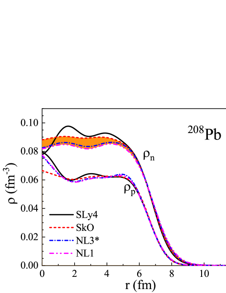
Figure 1: (Color online) Ground-state $\rho_{n}$ and $\rho_{p}$ for ²⁰⁸Pb calculated by the various models. The shaded part is shown to reproduce the experimental error bar of PREX-II data.

Besides the PVES experiment, the quasielastic ($p,n$) scattering is also sensitive to the nuclear isovector properties. Therefore, that scattering can be used to test $\Delta R_{np}$ Loc et al. (2014, 2017). Form Eqs. (15) and (16), one can see that $U_{\mathrm{IV}}$ is directly related to the $\Delta R_{np}$. However, the renormalization coefficients of the folded potential are undetermined in the calculation of scattering cross section. In the next part, we constrain the renormalization coefficients based on the $\Delta R_{np}$ of PREX-II results and the experimental data of the ($p,p$) and quasielastic ($p,n$) cross sections on ²⁰⁸Pb. With the fine-tuned folded potential, we further study the sensitivities of the ($p,p$) and ($p,n$) cross sections to the neutron density distribution $\rho_{n}$.

III.2 B. Complex folding model analysis

Next, we examine the ($p,p$) and ($p,n$) scattering cross sections within the complex folding model. The basic inputs for the folding model are the nuclear density distribution and the effective $NN$ interaction. The nuclear densities for Eqs. (15) and (16) are obtained from the mean-field models. For the effective $NN$ interaction, we choose the CDM3Y6 interaction Khoa et al. (2007a). The real part of the isoscalar density dependence of CDM3Y6 interaction $F_{\mathrm{IS}}^{\scriptscriptstyle V}(E,\rho)$ can be expressed as

$$F_{\mathrm{IS}}^{\scriptscriptstyle V}(E,\rho)=g(E)C_{0}\left[1+\alpha_{0}\exp\left(-\beta_{0}\rho\right)-\gamma_{0}\rho\right],$$ (22)

where the parameters combination $C_{0}$, $\alpha_{0}$, $\beta_{0}$ and $\gamma_{0}$ provides a nuclear incompressibility of $K\approx 252$ MeV Khoa et al. (2002). The energy dependence of $F_{\mathrm{IS}}^{\scriptscriptstyle V}(E,\rho)$ is contained in the factor $g$ changing linearly with energy $g(E)$$\approx 1-0.002E$. Given the successful application of such parametrized density dependence in numerous folding calculations, the imaginary part of such isoscalar density dependence $F_{\mathrm{IS}}^{\scriptscriptstyle W}(E,\rho)$ and isovector density dependence $F_{\mathrm{IV}}^{u}(E,\rho)$ are assumed to have the form inspired by $F_{\mathrm{IS}}^{\scriptscriptstyle V}(E,\rho)$

$$F_{\mathrm{IS}}^{\scriptscriptstyle W}(E,\rho)=C_{0}^{\scriptscriptstyle W}(E)\left[1+\alpha_{0}^{\scriptscriptstyle W}(E)\exp\left(-\beta_{0}^{\scriptscriptstyle W}(E)\rho\right)-\gamma_{0}^{\scriptscriptstyle W}(E)\rho\right],$$ (23)

$$F_{\mathrm{IV}}^{u}(E,\rho)=C_{1}^{u}(E)\left[1+\alpha_{1}^{u}(E)\exp\left(-\beta_{1}^{u}(E)\rho\right)-\gamma_{1}^{u}(E)\rho\right],$$ (24)

in which the parameters of $F_{\mathrm{IS}}^{\scriptscriptstyle W}(E,\rho)$ and $F_{\mathrm{IV}}^{u}(E,\rho)$ are assumed to be energy-dependent and are adjusted at each incident energy $E$. In Eqs. (15) and (16), the radial shapes of direct and exchange parts $v^{\mathrm{D(EX)}}$ of CDM3Y6 interaction are taken from the M3Y-Paris interaction as a combination of three Yukawa terms Anantaraman et al. (1983)

$$v_{\mathrm{IS(IV)}}^{\mathrm{D}(\mathrm{EX})}(s)=\sum_{v=1}^{3}Y_{\mathrm{IS(IV)}}^{\mathrm{D}(\mathrm{EX})}(v)\frac{\exp\left(-R_{v}s\right)}{R_{v}s},$$ (25)

where the Yukawa strengths can be found in Ref. Khoa et al. (2007a).

With Eqs. (22)-(25), the $V_{\mathrm{IS(IV)}}$ and $W_{\mathrm{IS(IV)}}$ of the folded potential in Eqs. (15) and (16) can be calculated explicitly and the $NA$ potential can be evaluated as

$$U_{\mathrm{N}}(R)=N_{V}\left[V_{\mathrm{IS}}(R)\pm N_{V1}V_{\mathrm{IV}}(R)\right]+iN_{W}\left[W_{\mathrm{IS}}(R)\pm W_{\mathrm{IV}}(R)\right],$$ (26)

where the ($+$) and ($-$) refer to neutrons and protons, respectively. The $N_{V(W)}$ and $N_{V1}$ are the renormalization coefficients established in this paper. The $N_{V(W)}$ and $N_{V1}$ are calibrated based on the experimental data for the ($p,p$) and ($p,n$) cross sections, assuming validity of the central $\Delta R_{np}$ value from PREX-II. The $N_{V1}$ is further tuned for different nuclei. The transition matrix element of Eq. (6) can be further expressed in terms of the folded potential $U_{\mathrm{IV}}$ as Khoa et al. (2014)

$$\langle n,Z+1|U(R)|p,Z\rangle =2\frac{\sqrt{|N-Z|}}{A}U_{1}(R)$$ (27)

$$=\frac{2}{\sqrt{|N-Z|}}U_{\mathrm{IV}}(R).$$

During the calibration process, $\rho_{n}$ is calculated using the NL3^∗ parameter set, because it gives a $\Delta R_{np}$ consistent with the central value of the PREX-II $\Delta R_{np}$ results. The best-fit renormalization coefficients at the incident energies of 35 MeV and 45 MeV are listed in Table 2. The corresponding parameters of CDM3Y6 interaction for incident energies at 35 MeV and 45 MeV are taken from Refs. Khoa et al. (2007a); com . Finally, the net scattering potential is obtained from the superposition of the $NA$ potential $U_{\mathrm{N}}$, the spin-orbital potential $U_{\mathrm{LS}}$ and the Coulomb potential $U_{\mathrm{C}}$.

Table 2: Renormalization coefficients $N_{V(W)}$ and $N_{V1}$ of the complex folded potential Eq. (26) at 35 MeV and 45 MeV, which are calibrated based on the experimental ($p,p$) and ($p,n$) cross sections, assuming that the central $\Delta R_{np}$ value from PREX-II is valid.

$E$			$N_{V}$			$N_{W}$			$N_{V1}$(48Ca)			$N_{V1}$(208Pb)
35			0.849			0.591			0.992			1.749
45			0.840			0.619			1.136			1.452

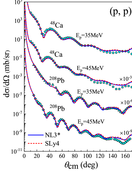
Figure 2: (Color online) Different ($p,p$) cross sections on ⁴⁸Ca and ²⁰⁸Pb targets at 35 MeV and 45 MeV from the calculations with the complex folded potential of Eq. (26), based on the nuclear densities calculated by the SHF and RMF models. The experimental data stem from Refs. McCamis et al. (1986); Van Oers et al. (1974).

The different ($p,p$) cross sections on ²⁰⁸Pb calculated with the complex folded potential of Eq. (26), at 35 MeV and 45 MeV, are shown in Fig. 2. It can be seen that the complex folded potential gives good ($p,p$) descriptions on cross section, which confirms the reliability of the complex folding model, especially here of its isoscalar component $U_{\mathrm{IS}}$. To provide insights, the ($p,p$) cross sections are obtained using both nuclear density distributions calculated with the NL3^∗ and SLy4 interaction. Note that $\Delta R_{np}$ calculated with these two interactions is different in Table 1, but the difference is hardly reflected in the ($p,p$) cross sections. This is because the ($p,p$) cross section is primarily related to the isoscalar net density, and only weakly to isovector density.

We further present the ($p,p$) cross sections on ⁴⁸Ca in Fig. 2, again using renormalization coefficients from Table 2. One can see that the theoretical results are in a reasonable agreement with experimental data. Importantly, the isoscalar renormalization coefficients used for ²⁰⁸Pb are reliable in calculating the ($p,p$) cross sections for the other nucleus. Similarly to ²⁰⁸Pb, little difference is observed when in the ($p,p$) cross sections of ⁴⁸Ca are calculated for different $\Delta R_{np}$. Concluding, while the ($p,p$) scattering can test the net density of the nucleus, it is not very sensitive to $\Delta R_{np}$.

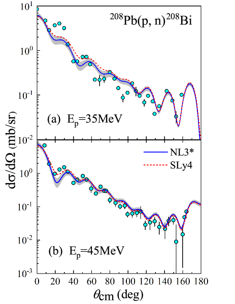
Figure 3: (Color online) Cross section for the quasielastic ²⁰⁸Pb($p,n$)²⁰⁸Bi reaction at 35 (a) and 45 (b) MeV. The experimental data from Ref. Doering et al. (1975) are represented by circles. DWBA calculations in the folding model of Eq. (26) are represented by lines, solid for the NL3^∗ interaction and dashed for SLy4. The shaded region represents the span of NL3^∗ results when the neutron radii corresponding to the nominal uncertainty in PREX-II.

The ($p,n$) cross sections on ²⁰⁸Pb obtained using NL3^∗ and SLy4 interactions at 35 MeV and 45 MeV are presented in Fig. 3. It can be seen that the calculations reproduce the general trend of the ($p,n$) experimental data, which demonstrates general validity of the isovector part $U_{\mathrm{IV}}$ of the $NA$ potential. There are evident differences between the predictions from these two models in the region $\theta=20^{\circ}\mbox{-}80^{\circ}$, which indicates that the effects of isovector density on ($p,n$) reaction are more obvious than on ($p,p$). This is because the ($p,n$) cross section is dominated by the $U_{\mathrm{IV}}$ component, which is connected to the nuclear isovector density and, thus, magnifies the effects of $\Delta R_{np}$.

As the $\Delta R_{np}$ calculated for NL3^∗ corresponds just to the central value of the $\Delta R_{np}$ result of PREX-II, we can explore the whole range of PREX-II uncertainty by stretching $\rho_{n}$ from NL3^∗ with a factor $\lambda$ Liu et al. (2013), i.e., carrying out transformation for the neutron density $\rho_{n}(r)\rightarrow\lambda^{-3}\rho_{n}\left(r/\lambda\right)$. With this method, the neutron radius is scaled by $\lambda$:

$$R_{n}^{\prime}=\sqrt{\int 4\pi r^{4}\frac{1}{\lambda^{3}}\rho_{n}\left(\frac{r}{\lambda}\right)dr}=\lambda\cdot R_{n}.$$

By choosing different $\lambda$, we can span the full range of nominal uncertainty for the PREX-II $R_{n}$ result, and the corresponding ($p,n$) cross sections are shown by the shaded areas in Fig. 3. One can see that the effects on ($p,n$) caused by the modifications of $\rho_{n}$ are significant over the uncertainty of PREX-II result.

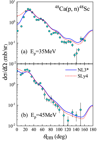
Figure 4: (Color online) Same as the Fig. 3, but for the quasielastic ⁴⁸Ca($p,n$)⁴⁸Sc reaction.

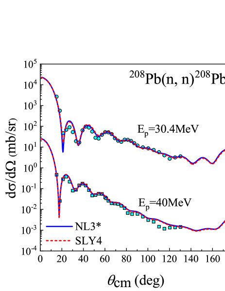
Figure 5: (Color online) Different ($n,n$) cross sections on ²⁰⁸Pb targets at 30.4 MeV and 40 MeV from the calculations with the complex folded potential of Eq. (26), based on the nuclear densities calculated by the SHF and RMF models. The experimental data stem from Ref. DeVito et al. (2012).

Besides the ²⁰⁸Pb target, the theoretical cross sections for the ⁴⁸Ca($p,n$)⁴⁸Sc reaction are also presented in Fig. 4, using the renormalization coefficients in Table 2. In the figure, one can again see that the general trend of theoretical results agrees with the experiment data, which supports the use of the renormalization coefficients. A further comparative study in Fig. 4 indicates that the NL3^∗ results agree better with the ($p,n$) data than SLy4, especially in the forward direction. However, the renormalization coefficients are primarily based on the experimental result from PREX-II in the current paper. After the experimental $\Delta R_{np}$ result of ⁴⁸Ca is updated, more universal renormalization coefficients can be obtained, which are helpful for the analyses in this paper.

With the exception of the ($p,p$) and ($p,n$) scattering, the elastic neutron ($n,n$) scattering is also considered to prove the consistency of the folded potential. The elastic neutron ($n,n$) cross sections on ²⁰⁸Pb at 30.4 MeV and 40 MeV are shown in Fig. 5. In analogy with the ($p,p$) scattering, the complex folded potential of Eq. (26) is renormalized at different incident energies to obtain $N_{V}\approx 0.80$ and $N_{W}\approx 0.65\mbox{-}0.75$. From Fig. 5, it can be seen that the complex folded potential of Eq. (26) gives good ($n,n$) descriptions on cross section, which indicate the validity of the complex folded potential on ($n,n$) scattering. Therefore, our results demonstrate the consistency among the charge-exchange effective interaction, the proton and the neutron folded potential in our calculations.

The theoretical results in Figs. 3 and 4 together illustrate that the complex folded potential can reflect differences in $\rho_{n}$ on the ($p,n$) cross section. However, the renormalization coefficient $N_{V1}$ needs to be readjusted for different nuclei, which indicates that the complex folding model has some limitations as far as its universality is concerned.

III.3 C. Hybrid folding model analysis

The $N_{V1}$ factor of the complex folding model has been a function of the mass number $A$ of nucleus. To retreat in the renormalizations carried out from our side, we use the hybrid folded potential:

$$U_{\mathrm{N}}(R)=N_{V}\left[V_{\mathrm{IS}}(R)-N_{V1}V_{\mathrm{IV}}(R)\right]+i\left[W_{0}(R)-W_{1}(R)\right],$$ (28)

where the $V_{\mathrm{IS}}$ and $V_{\mathrm{IV}}$ terms retain the folded potential, and the imaginary part is replaced by that from a phenomenological optical model potential. Specifically in Eq. (28), the $W_{0}(R)$ and $W_{1}(R)$ are the isoscalar and isovector parts of the imaginary Koning-Delaroche (KD) potential Koning and Delaroche (2003), respectively. The KD global systematics covers a wide range of target masses and energies. Similar to the case of the complex folded potential, we calibrate $N_{V(V1)}$ of the hybrid folded potential on the experimental ($p,p$) and ($p,n$) cross sections on ²⁰⁸Pb, assuming validity of the central value of the $\Delta R_{np}$ PREX-II result, i.e., NL3^∗ densities. The calibrated $N_{V(V1)}$ at the incident energies of 35 MeV and 45 MeV are given in Table 3. In this way, the renormalization coefficients are universal for different nuclei, but depend on energy.

Table 3: Renormalization coefficients $N_{V}$ and $N_{V1}$ of the hybrid folded potential of Eq. (28) at 35 MeV and 45 MeV, which are calibrated based on the experimental ($p,p$) and ($p,n$) cross sections, assuming the validity of the central value of $\Delta R_{np}$ from PREX-II.

			$E$									$N_{V}$									$N_{V1}$
			35									0.902									0.908
			45									0.936									1.105

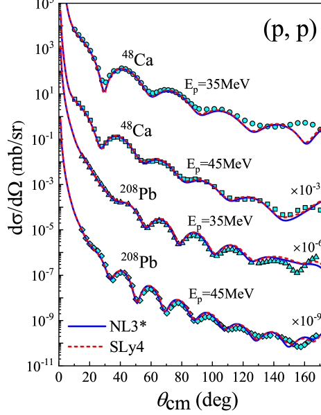
Figure 6: (Color online) Same as the Fig. 2, but with calculations in the hybrid folded potential Eq. (28).

The ($p,p$) cross sections on ⁴⁸Ca and ²⁰⁸Pb, calculated with the hybrid folded potential Eq. (28) and the renormalization coefficients in Table 3 using NL3^∗ and SLy4 interactions, are presented in Fig. 6. The theoretical cross sections are in good agreement with the experimental data, which validates the use of the hybrid folding model with the calibrated renormalization coefficients. From Fig. 6 one can see that the effects of different $\rho_{n}$ on ($p,p$) cross sections are rather minute. This can be attributed to the fact that the impact of $V_{\mathrm{IV}}$ on the ($p,p$) cross sections is relatively small. In comparing the results in Fig. 2 and Fig. 6, one can observe clear differences between the ($p,p$) cross sections calculated with the complex folded potential and hybrid folded potential, especially in the backward region. These are due to the surface term of the imaginary part of isoscalar potential $U_{\mathrm{IS}}$. Notably, while the real part of the hybrid folded potential is quite close in shape and strength to the real KD potential, the imaginary part is quite different.

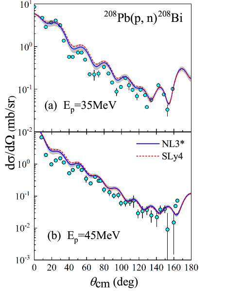
Figure 7: (Color online) Same as Fig. 3, but for the hybrid folded potential of Eq. (28).

With the renormalization coefficients of Table 3, the theoretical ($p,n$) scattering cross sections on ²⁰⁸Pb have been again calculated and are presented in Fig. 7. By stretching neutron density $\rho_{n}$, the uncertainty in $R_{n}$ in the PREX-II measurement is again mapped onto the shaded areas. In comparing Fig. 3 and Fig. 7, one can see that the hybrid folded potential gives better descriptions of the ($p,n$) data than the complex folded potential, which can be attributed to the surface term of the hybrid folded potential. Specifically, the imaginary KD potential can be represented by a combination of volume and surface terms. The imaginary folded potential only exhibits the volume character, since it is constructed based on the nucleon optical potential calculated by the nuclear matter. Therefore, the imaginary folded potential cannot appropriately explain the surface absorption of the transfer reactions caused by inelastic scattering and reflects only the nature of the volume Khoa et al. (2007a). However, all phenomenological potentials have a surface-peaked form at low energies, which slowly changes to a volume form as the energy increases. In the range of incident energies studied in this paper, the surface absorption is still very strong. Thus, the ($p,n$) cross section given by the hybrid folded potential of Eq. (28) is more accurate for the probe of the neutron density distribution.

In comparing the theoretical results from the NL3^∗ and SLy4 interactions in Fig. 7, it may be seen that the ($p,n$) cross sections predicted by the hybrid folded potential are also sensitive to $\rho_{n}$. This is because the transition strength of the ($p,n$) reaction to IAS is determined entirely by the isovector part in hybrid folded potential, although only the real part of isovector potential is now calculated from the derived nuclear density distribution. Therefore, even the hybrid folding model can also be used to study neutron density distribution $\rho_{n}$. Besides, the hybrid folding model may be viewed as a more objective inference method, since the renormalization coefficients are the same for different target nucleus. In the following, we progress to using the hybrid folding model in testing the impacts of the neutron properties of ⁴⁸Ca.

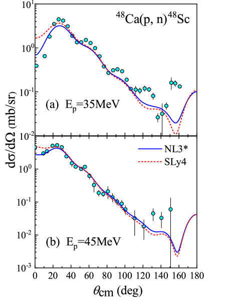
Figure 8: (Color online) Same as Fig. 4, but for the hybrid folded potential of Eq. (28).

In Fig. 8, we present the ($p,n$) cross sections on ⁴⁸Ca obtained in the hybrid folded potential at 35 MeV and 45 MeV, using the renormalization coefficients. It can be observed in this figure that the results from the hybrid folded potential provide good description of the ⁴⁸Ca($p,n$)⁴⁸Sc quasielastic reaction data, which supports the universality of the renormalization coefficients in Table 3. In addition, we find that the ($p,n$) cross sections calculated with the NL3^∗ and SLy4 interactions significantly differ in the regions $\theta=0^{\circ}\mbox{-}40^{\circ}$ and $\theta=80^{\circ}\mbox{-}160^{\circ}$. Therefore, we can effectively constrain the neutron properties following the hybrid folding model. In Fig. 8, one can see that the results of NL3^∗ parameter set are generally closer to the ($p,n$) data, especially in the forward and backward angles. This finding is consistent with the conclusions of the complex folding model analysis.

IV IV. Conclusion

The neutron skin thickness $\Delta R_{np}$ and the neutron density distribution $\rho_{n}$ are fundamental nuclear properties, which attracted increased attention recently. Relying on the relation between $\rho_{n}$ and the quasielastic ($p,n$) cross section in this paper, we have investigated the impact of neutron properties in the context of the available experimental values.

In calculating the neutron properties in the RMF and SHF models, we found that the $\Delta R_{np}$ and $\rho_{n}$ can differ significantly among different parameter sets. The elastic ($p,p$) and quasielastic ($p,n$) cross sections of ²⁰⁸Pb have been investigated in the combination of the DWBA method and the folding model. The renormalization coefficients for the folded potential have been calibrated using the experimental ($p,p$) and ($p,n$) data assuming central value of the neutron skin thickness $\Delta R_{np}$ of ²⁰⁸Pb in the PREX-II measurement. The isovector potential determines the transition strength of the initial state to IAS in charge-exchange ($p,n$) reactions. Therefore, the accurate measurement of the ($p,n$) cross sections can serve as a sensitive probe of the neutron skin thickness $\Delta R_{np}$ and the nuclear isovector density. Results in this paper also indicate that the ($p,n$) cross section is sensitive to the nuclear neutron density distribution $\rho_{n}$. By further comparing the results of the complex and hybrid folding model, we found that the ($p,n$) reaction can be more reasonable described by introducing the surface term into the folded potential.

With the renormalization coefficients calibrated in this paper, the ($p,n$) cross sections of ⁴⁸Ca have also been calculated in the folding model for different neutron density distribution $\rho_{n}$. Theoretical quasielastic ($p,n$) cross sections have been compared with the experimental data. It has been observed that the results of NL3* parameter set are consistent with the experimental data. The results of this paper can provide counter reference for the CREX experiment. Besides, our investigations on charge exchange reactions are also helpful for other fields of nuclear structure and nuclear reactions.

References

- Danielewicz et al. (2002) P. Danielewicz, R. Lacey, and W. G. Lynch, Science 298, 1592 (2002).
- Centelles et al. (2009) M. Centelles, X. Roca-Maza, X. Viñas, and M. Warda, Phys. Rev. Lett. 102, 122502 (2009).
- Steiner et al. (2013) A. W. Steiner, J. M. Lattimer, and E. F. Brown, Astrophys. J. Lett. 765, L5 (2013).
- Tsang et al. (2020) C. Y. Tsang, M. B. Tsang, P. Danielewicz, W. G. Lynch, and F. J. Fattoyev, Phys. Rev. C 102, 045808 (2020).
- Tsang et al. (2012) M. B. Tsang, J. R. Stone, F. Camera, P. Danielewicz, S. Gandolfi, K. Hebeler, C. J. Horowitz, J. Lee, W. G. Lynch, and Z. Kohley et al., Phys. Rev. C 86, 015803 (2012).
- Giacalone (2020) G. Giacalone, Phys. Rev. C 102, 024901 (2020).
- Patton et al. (2012) K. Patton, J. Engel, G. C. McLaughlin, and N. Schunck, Phys. Rev. C 86, 024612 (2012).
- Tagami et al. (2021) S. Tagami, T. Wakasa, J. Matsui, M. Yahiro, and M. Takechi, Phys. Rev. C 104, 024606 (2021).
- Trzcińska et al. (2001) A. Trzcińska, J. Jastrzȩbski, P. Lubiński, F. J. Hartmann, R. Schmidt, T. von Egidy, and B. Kłos, Phys. Rev. Lett. 87, 082501 (2001).
- Brown et al. (2007) B. A. Brown, G. Shen, G. C. Hillhouse, J. Meng, and A. Trzcińska, Phys. Rev. C 76, 034305 (2007).
- Kłos et al. (2007) B. Kłos, A. Trzcińska, J. Jastrzȩbski, T. Czosnyka, M. Kisieliński, P. Lubiński, P. Napiorkowski, L. Pieńkowski, F. J. Hartmann, and B. Ketzer et al., Phys. Rev. C 76, 014311 (2007).
- Abrahamyan et al. (2012) (PREX Collaboration) S. Abrahamyan et al. (PREX Collaboration), Phys. Rev. Lett. 108, 112502 (2012).
- Fattoyev et al. (2018) F. J. Fattoyev, J. Piekarewicz, and C. J. Horowitz, Phys. Rev. Lett. 120, 172702 (2018).
- Adhikari et al. (2021) (PREX Collaboration) D. Adhikari et al. (PREX Collaboration), Phys. Rev. Lett. 126, 172502 (2021).
- Reed et al. (2021) B. T. Reed, F. J. Fattoyev, C. J. Horowitz, and J. Piekarewicz, Phys. Rev. Lett. 126, 172503 (2021).
- Androić et al. (2022) D. Androić, D. S. Armstrong, K. Bartlett, R. S. Beminiwattha, J. Benesch, F. Benmokhtar, J. Birchall, R. D. Carlini, J. C. Cornejo, and S. C. Dusa et al., Phys. Rev. Lett. 128, 132501 (2022).
- Adhikari et al. (2022) D. Adhikari, H. Albataineh, D. Androic, K. Aniol, D. S. Armstrong, T. Averett, C. A. Gayoso, S. Barcus, V. Bellini, and R. S. Beminiwattha et al., Phys. Rev. Lett. 128, 142501 (2022).
- Zegers et al. (2003) R. G. T. Zegers, H. Abend, H. Akimune, A. M. van den Berg, H. Fujimura, and H. Fujita et al., Phys. Rev. Lett. 90, 202501 (2003).
- Zegers et al. (2006) R. G. T. Zegers, H. Akimune, S. M. Austin, D. Bazin, A. M. van den Berg, and G. P. A. Berg et al., Phys. Rev. C 74, 024309 (2006).
- Loc et al. (2014) B. M. Loc, D. T. Khoa, and R. G. T. Zegers, Phys. Rev. C 89, 024317 (2014).
- Loc et al. (2017) B. M. Loc, N. Auerbach, and D. T. Khoa, Phys. Rev. C 96, 014311 (2017).
- Satchler (1983) G. R. Satchler, Direct Nuclear Reactions (Clarendon, Oxford, 1983).
- Phan Nhut Huan et al. (2021) Phan Nhut Huan, Nguyen Le Anh, Bui Minh Loc, and I. Vidaña, Phys. Rev. C 103, 024601 (2021).
- Khoa et al. (2007a) D. T. Khoa, H. S. Than, and D. C. Cuong, Phys. Rev. C 76, 014603 (2007a).
- Varner et al. (1991) R. L. Varner, W. J. Thompson, T. L. McAbee, E. J. Ludwig, and T. B. Clegg, Phys. Rep. 201, 57 (1991).
- Koning and Delaroche (2003) A. J. Koning and J. P. Delaroche, Nucl. Phys. A 713, 231 (2003).
- Satchler and Love (1979) G. R. Satchler and W. G. Love, Phys. Rep. 55, 183 (1979).
- Wiringa et al. (1995) R. B. Wiringa, V. G. J. Stoks, and R. Schiavilla, Phys. Rev. C 51, 38 (1995).
- Somasundaram et al. (2021) R. Somasundaram, C. Drischler, I. Tews, and J. Margueron, Phys. Rev. C 103, 045803 (2021).
- Stoks et al. (1994) V. G. J. Stoks, R. A. M. Klomp, C. P. F. Terheggen, and J. J. deSwart, Phys. Rev. C 49, 2950 (1994).
- Khoa et al. (2002) D. T. Khoa, E. Khan, G. Colò, and N. Van Giai, Nucl. Phys. A 706, 61 (2002).
- Khoa et al. (2007b) D. T. Khoa, W. von Oertzen, H. G. Bohlen, and S. Ohkubo, J. Phys. G: Nucl. Part. Phys. 34, R111 (2007b).
- Deng and Ren (2017) D. Deng and Z. Ren, Phys. Rev. C 96, 064306 (2017).
- Hamada (2018) S. Hamada, Phys. Part. Nucl. Lett. 15, 143 (2018).
- Durant et al. (2020) V. Durant, P. Capel, and A. Schwenk, Phys. Rev. C 102, 014622 (2020).
- Khoa et al. (2016) D. T. Khoa, N. H. Phuc, D. T. Loan, and B. M. Loc, Phys. Rev. C 94, 034612 (2016).
- Kurasawa and Suzuki (2019) H. Kurasawa and T. Suzuki, Prog. Theor. Exp. Phys. 2019, 113D01 (2019).
- Naito et al. (2021) T. Naito, G. Colò, H. Liang, and X. Roca-Maza, Phys. Rev. C 104, 024316 (2021).
- Wang et al. (2021a) X. Wang, Q. Niu, J. Zhang, M. Lyu, J. Liu, C. Xu, and Z. Ren, Sci. China Phys. Mech. Astron. 64, 292011 (2021a).
- Niu et al. (2022) Q. Niu, J. Liu, Y. Guo, C. Xu, M. Lyu, and Z. Ren, Phys. Rev. C 105, L051602 (2022).
- Meucci et al. (2014) A. Meucci, M. Vorabbi, C. Giusti, and P. Finelli, Phys. Rev. C 90, 027301 (2014).
- Liu et al. (2017a) J. Liu, C. Xu, and Z. Ren, Phys. Rev. C 95, 044318 (2017a).
- Wang et al. (2020) L. Wang, J. Liu, T. Liang, Z. Ren, C. Xu, and S. Wang, J. Phys. G: Nucl. Part. Phys. 47, 025105 (2020).
- Wang et al. (2021b) L. Wang, J. Liu, R. Wang, M. Lyu, C. Xu, and Z. Ren, Phys. Rev. C 103, 054307 (2021b).
- Roca-Maza et al. (2011) X. Roca-Maza, M. Centelles, X. Viñas, and M. Warda, Phys. Rev. Lett. 106, 252501 (2011).
- Fröbrich and Lipperheide (1996) P. Fröbrich and R. Lipperheide, Theory of nuclear reactions (Oxford University Press, New York, 1996).
- Horowitz et al. (2014) C. J. Horowitz, K. S. Kumar, and R. Michaels, Eur. Phys. J. A 50, 48 (2014).
- Xu et al. (2008) C. Xu, Z. Ren, and Y. Guo, Phys. Rev. C 78, 044329 (2008).
- Deng et al. (2019) D. Deng, Z. Ren, and N. Wang, Phys. Lett. B 795, 554 (2019).
- Xu and Li (2010) C. Xu and B. A. Li, Phys. Rev. C 81, 064612 (2010).
- Khoa et al. (2014) D. T. Khoa, B. M. Loc, and D. N. Thang, Eur. Phys. J. A 50, 34 (2014).
- Bertulani and Danielewicz (2004) C. A. Bertulani and P. Danielewicz, Introduction to Nuclear Reactions (Institute of Physics Publishing, London, 2004).
- Danielewicz and Kurata-Nishimura (2022) P. Danielewicz and M. Kurata-Nishimura, Phys. Rev. C 105, 034608 (2022).
- Danielewicz et al. (2017) P. Danielewicz, P. Singh, and J. Lee, Nucl. Phys. A 958, 147 (2017).
- Tan et al. (2021) N. H. Tan, D. T. Khoa, and D. T. Loan, Eur. Phys. J. A 57, 1 (2021).
- Loan et al. (2020) D. T. Loan, D. T. Khoa, and N. H. Phuc, J. Phys. G: Nucl. Part. Phys. 47, 035106 (2020).
- Anantaraman et al. (1983) N. Anantaraman, H. Toki, and G. F. Bertsch, Nucl. Phys. A 398, 269 (1983).
- Stoitsov et al. (2007) M. V. Stoitsov, J. Dobaczewski, R. Kirchner, W. Nazarewicz, and J. Terasaki, Phys. Rev. C 76, 014308 (2007).
- Todd-Rutel and Piekarewicz (2005) B. G. Todd-Rutel and J. Piekarewicz, Phys. Rev. Lett. 95, 122501 (2005).
- Liu et al. (2017b) J. Liu, C. Xu, S. Wang, and Z. Ren, Phys. Rev. C 96, 034314 (2017b).
- Angeli and Marinova (2013) I. Angeli and K. P. Marinova, At. Data Nucl. Data Tables 99, 69 (2013).
- Wang et al. (2021c) M. Wang, W. J. Huang, F. G. Kondev, G. Audi, and S. Naimi, Chin. Phys. C 45, 030003 (2021c).
- (63) Private communication with D. T. Khoa.
- McCamis et al. (1986) R. H. McCamis, T. N. Nasr, J. Birchall, N. E. Davison, W. T. H. Van Oers, P. J. T. Verheijen, R. F. Carlson, A. J. Cox, B. C. Clark, E. D. Cooper, S. Hama, and R. L. Mercer, Phys. Rev. C 33, 1624 (1986).
- Van Oers et al. (1974) W. T. H. Van Oers, H. Haw, N. E. Davison, A. Ingemarsson, B. Fagerström, and G. Tibell, Phys. Rev. C 10, 307 (1974).
- Doering et al. (1975) R. R. Doering, D. M. Patterson, and A. Galonsky, Phys. Rev. C 12, 378 (1975).
- Liu et al. (2013) J. Liu, Z. Ren, and T. Dong, Nucl. Phys. A 900, 1 (2013).
- DeVito et al. (2012) R. P. DeVito, D. T. Khoa, S. M. Austin, U. E. P. Berg, and B. M. Loc, Phys. Rev. C 85, 024619 (2012).