Position tracking of a varying number of sound sources with
sliding permutation invariant training

Tóm tắt nội dung

Machine-learning-based sound source localization (SSL) methods have shown strong performance in challenging acoustic scenarios. However, little work has been done on adapting such methods to track consistently multiple sources appearing and disappearing, as would occur in reality. In this paper, we present a new training strategy for deep learning SSL models with a straightforward implementation based on the mean squared error of the optimal association between estimated and reference positions in the preceding time frames. It optimizes the desired properties of a tracking system: handling a time-varying number of sources and ordering localization estimates according to their trajectories, minimizing identity switches (IDSs). Evaluation on simulated data of multiple reverberant moving sources and on two model architectures proves its effectiveness in reducing identity switches without compromising frame-wise localization accuracy.

Index Terms—  Sound source tracking (SST), deep learning, permutation invariant training (PIT)

1 Introduction

Machine-Learning-based sound source localization (SSL) using neural networks (NNs) has been an intensely active research field during the last years [1] but with a fair amount of problems still open. A major one is how to deal with the common real-world scenario that the number of active sources in the scene varies, as sources appear and disappear dynamically, with proposed solutions employing either simultaneous classification [2] or assigning temporal source activity probabilities for a fixed number of model outputs [3, 4]. Another closely related open problem is associating new location estimates to the appropriate model output in the case of multiple simultaneous sources, such that the same output provides a consistent sequence of locations tracking the trajectory of the same source. The above combined tracking objectives are essential in making deep-learning localizers useful in further downstream tasks, such as beamforming, source separation, or robot audition, that can utilize the location information of multiple sources in the scene.

Multi-source localization has been tackled in the literature mainly using a classification framework, e.g. [5, 6], indicating source presence probabilities on a grid of locations, which can naturally accommodate a time-varying number of sources but without providing assignment between detected spatial labels and source identities or trajectories. Proposals that localize multiple sources using regression follow mainly a simultaneous localization and detection framework (SELD) [7, 8] which naturally associates a source trajectory to temporal activity of a target class, but only in the case that there are no multiple sources of the same class active simultaneously. A few regression-based localization works have aimed to tackle that problem using a frame-wise permutation invariant training (PIT) strategy, either in a SELD context [9, 10] or in a pure SSL one [11, 12]. PIT allows effective training of regression-based multi-source localization, but without promoting the tracking objectives outlined above.

A recent attempt aiming to optimize directly tracking objectives for SSL models is presented in [4], where a NN is trained to infer the frame-wise assignments between estimated and ground truth directions-of-arrival (DOAs), which are further used to construct differentiable versions of multi-object-tracking metrics [13]. Based on those, tracking losses are back-propagated to the outputs of the localization model during its training. While the method is shown to be effective, using an auxiliary NN to compute the loss function adds implementation and training complexity, with harder-to-interpret gradients that are more prone to vanishing effects.

In this paper, we propose a modification to PIT that penalizes IDSs at each frame by considering the source permutation that minimizes the MSE over a number of preceding frames. Additionally, we show that if the SSL model provides DOAs in the activity-coupled DOA (ACCDOA) representation [8], which joins localization and detection information by scaling a DOA vector by its probability of belonging to an active source, then the proposed training also minimizes source misses and false positives. Hence, it makes the model reactive to variable source conditions and optimizes all the tracking objectives outlined earlier. This new PIT strategy is easy to implement, has a very similar computational cost to the standard PIT and, being based on backpropagating the MSE of one of the possible permutations of the estimated DOAs, it generates gradients that are strong and easy to interpret.

2 Permutation Invariant Training for sound source tracking

When we want to train a sound source tracking (SST) model in a supervised manner and we cannot apply any criteria to classify and order the sources, we have to face the permutation invariance of the sources; i.e., we cannot directly compare the m-th trajectory estimated by the model $\hat{\mathbf{y}}_{m}(t)$ with the m-th trajectory of our ground-truth dataset $\mathbf{y}_{m}(t)$ since the model cannot infer the ground-truth order of the trajectories. This is a well-known issue in the speech separation field, where permutation invariant training (PIT) was first proposed [14].

All the PIT strategies propose finding a permutation $\sigma:m\rightarrow\sigma_{m},\;\forall m\in\{0,...,M-1\}$ according to certain optimization criteria to reorder the outputs of the neural network and then use it to compare the estimated and ground-truth trajectories. When using ACCDOA vectors to represent the DOA and the activity of the sources, we can use the mean squared error (MSE) as the loss function to train our models:

$$L_{PIT}=\frac{1}{TM}\sum_{t=0}^{T-1}\sum_{m=0}^{M-1}\lVert\mathbf{y}_{m}(t)-\hat{\mathbf{y}}_{{\sigma}_{m}(t)}(t)\rVert^{2}$$ (1)

where $M$ is the maximum number of trajectories that the model can estimate, $T$ is the number of time frames in the scene, and $\rVert\cdot\rVert$ is the Euclidean norm operator. In the case of having a number of ground-truth trajectories lower than $M$, we can just add as many 0-norm padding trajectories.

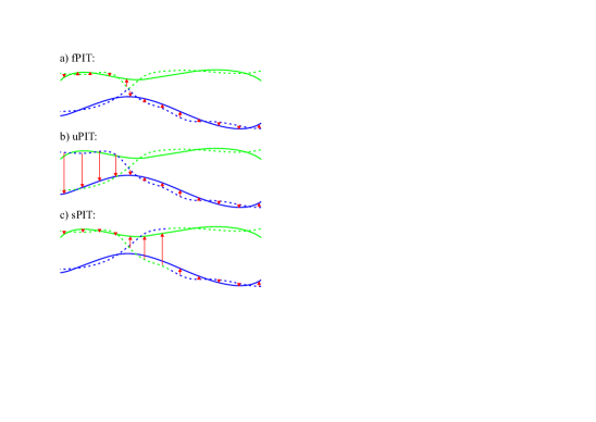
Fig. 1: Examples of 1D trajectories and the result of applying the different PIT strategies. The dashed lines represent the estimates and their color how every PIT pair them with the ground-truth trajectories (solid lines). The red arrows represent the gradients of the MSE of every pairing w.r.t. the first estimated trajectory.

2.1 Frame-level Permutation Invariant Training (fPIT)

The original PIT [14] applied to SSL [11, 12], which we will call frame-level PIT (fPIT), finds the permutation of the estimated sources that minimizes the matching error between the estimated and the ground-truth DOAs for every time frame:

$$\sigma^{f}(t)=\operatorname*{arg\,min}_{\sigma\in\Pi_{M}}\sum_{m=0}^{M-1}\lVert\mathbf{y}_{m}(t)-\hat{\mathbf{y}}_{\sigma_{m}}(t)\rVert$$ (2)

where $\Pi_{M}$ is the set of all the permutations $\sigma:i\rightarrow\sigma_{i}$ of $M$ elements. This optimization problem can be solved by computing the $M\times M$ distance matrices $\mathbf{D}(t)$ with elements $d_{ij}(t)=\lVert\mathbf{y}_{i}(t)-\hat{\mathbf{y}}_{j}(t)\rVert$ and applying the Hungarian algorithm over them to find the optimal permutation for every time frame.

Using $\sigma^{f}(t)$ in (1) allows us to solve the permutation invariance problem but, as we can see in Fig. 1a, fPIT does not penalize at all the IDSs. Instead, its gradients push the model to do these switches as fast as possible so that estimations are close to a ground-truth trajectory at all time frames. Therefore, if we want to keep the identity of every output stable during tracking, we need to add post-processing stages to fix the IDSs.

2.2 Utterance-level Permutation Invariant Training (uPIT)

In order to penalize the IDSs, utterance-level PIT (uPIT) [15] proposes finding the permutation that minimizes the error for a whole speech utterance or some other longer recording unit of interest, instead of a different one for every time frame:

$$\sigma^{u}=\operatorname*{arg\,min}_{\sigma\in\Pi_{M}}\sum_{t=0}^{T-1}\sum_{m=0}^{M-1}\lVert\mathbf{y}_{m}(t)-\hat{\mathbf{y}}_{\sigma_{m}}(t)\rVert$$ (3)

where $T$ is the number of time frames of the acoustic scene. In this case, we only need to apply the Hungarian algorithm once per acoustic scene after computing the time average of the matrices $\mathbf{D}(t)$.

Replacing $\sigma^{f}(t)$ by $\sigma^{u}$ in (1) indeed penalizes the presence of IDSs since all the frames where the output ACCDOAs do not follow the main identity assignment count as completely wrong estimations. However, as we can see in Fig. 1b, this penalization is excessive, being able to penalize situations that can not be solved by causal systems or generating gradients too much time after the IDS when, in most situations, it would be preferred to focus and keep tracking on the new identities rather than switching them again. Our experiments in using uPIT for multi-source tracking showed that it can easily generate a wide local minimum in the loss function that corresponds to estimating all DOAs in the middle of the active sources. That effect makes effective model training impossible, especially for long scenes of variable multiple sources.

3 Sliding Permutation Invariant Training (sPIT)

To overcome the limitations of both fPIT and uPIT, we propose a new PIT strategy that we call sliding PIT (sPIT) which consists in choosing, for every time frame, the optimal permutation for the last $T_{avg}$ frames, i.e., for a causal sliding window of length $T_{avg}$:

$$\sigma^{s}(t)=\operatorname*{arg\,min}_{\sigma\in\Pi_{M}}\sum_{k=0}^{T_{avg}-1}\sum_{m=0}^{M-1}\lVert\mathbf{y}_{m}(t-k)-\hat{\mathbf{y}}_{\sigma_{m}}(t-k)\rVert$$ (4)

In order to obtain $\sigma^{s}(t)$ for every time frame, we can follow the same procedure as in the fPIT but applying a causal moving average of length $T_{avg}$ over the elements of $\mathbf{D}(t)$ before computing the Hungarian algorithm, so the computational complexity is virtually the same. It is worth mentioning that, in the case of training non-causal trackers, we could replace the causal moving window in (4) by a centered window.

As shown in Fig. 1c, the sPIT penalizes an estimation if it does not follow the main source assignment of the last $T_{avg}$, while it stops penalizing an IDS after a maximum of $T_{avg}$ frames and focuses on maintaining the new identities. Hence, the global minimum of the loss function corresponds to a solution without any IDSs that also avoids the training converging to the useless local minima generated by uPIT, estimating all DOAs in the middle point of the active sources.

In addition, when used over ACCDOA vectors, if the number of estimated sources is lower than the actual number, one of the estimated ACCDOA vectors whose norm is lower than the detection threshold will be paired with the ground-truth ACCDOA vector of the missed source and the gradients of (1) will pull that estimated ACCDOA towards it. In a similar manner, in the case of a false positive, the gradients will pull the false-positive ACCDOA towards 0. Hence, sPIT is able to optimize both source detections and consistent source assignments that we expect from a competent SST system.

4 Evaluation

4.1 Experiment design

To evaluate sPIT, we have trained and evaluated a fully convolutional model and a convolutional model with recurrent layers at its end using simulated scenarios with up to three active sources at the same time. We trained the models using fPIT, uPIT, and sPIT, but we do not include the uPIT results since it did not converge to any proper solution.

We have used a synthetic dataset similar to the one used in [16], but with the number of sources varying during each $20\text{\,}\mathrm{s}$ scene. Every $200\text{\,}\mathrm{ms}$ new sources could birth with a rate of 0.06, 0.04, or 0.02 depending on whether there are already 0, 1, or 2 active sources. Once they are born, they could have a minimum duration of $2\text{\,}\mathrm{s}$ and, after that, every $200\text{\,}\mathrm{ms}$ they could die with a probability of 0.02.

For each trajectory, we randomly chose a starting and ending point and connect them using sinusoidal functions in the three Cartesian coordinates and simulate the room acoustics in a reverberation range from $T_{60}=$ 0.2 to $1.3\text{\,}\mathrm{s}$ using the Image Source Method [17] with utterances from the LibriSpeech dataset [18] as source signals and a 12-microphone array designed to be mounted over a NAO robot head [19] as receiver.

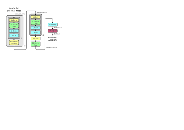
Fig. 2: Architecture of the icoCNN used for evaluation. B is the batch size, T is the number of temporal frames of the acoustic scenes, $H=2^{r}=8$ and $W=2^{r+1}=16$ are the height and the width of the projections of the icosahedral grid.

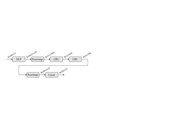
Fig. 3: Architecture of the RNN used after the icoCNN for evaluation.

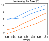
(a)

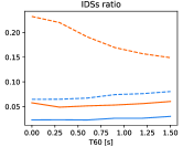
(b)

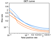
(c)

(d)

Fig. 4: Evaluation metrics obtained using fPIT and sPIT to train the two analyzed models.

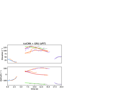
(a)

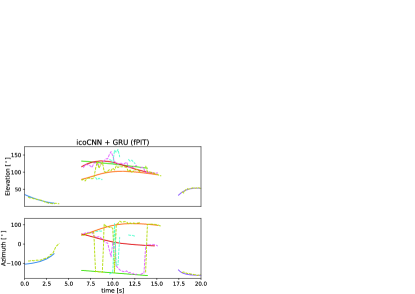
(b)

Fig. 5: Example of an evaluation acoustic scene and output of the icoCNN + GRU model trained with sPIT and fPIT. The solid lines represent the ground-truth trajectories and the dashed lines the estimations.

For the fully convolutional model, we have modified the model presented in [16] to make it work in multi-source scenarios. The original model computed SRP-PHAT power maps defined on a tessellated icosahedron using frames of 4096 samples with a sampling rate of $16\text{\,}\mathrm{kHz}$ and analyzed them with an icosahedral CNN (icoCNN) [20] using 1D temporal convolutions for tracking. The icoCNN transformed the power maps into an icosahedral probability distribution whose expected value, computed with a Soft-ArgMax layer, corresponded to the estimated DOA. In order to adapt the model to handle the multi-source case, we just increased the number of channels of the last convolutional layer from 1 to $M$. The general architecture of this model is represented in Fig. 2, with all the convolutions having 128 channels except for the last temporal convolution having $M$. We used input maps of resolution $r=3$ (i.e., with 630 grid points) and temporal convolutions with kernels of size 5, so the model had a temporal receptive field of $7.17\text{\,}\mathrm{s}$.

Since most of the SST models in the literature include recurrent layers after their CNNs [2, 6, 4, 8, 11], we also evaluate the same model adding the RNN depicted in Fig. 3 at its end. It uses a multi-layer perceptron (MLP) to expand the 3D ACCDOA vectors generated by the convolutional model to a space of 128 dimensions. It then concatenates the $M$ representations of every trajectory and applies two gated recurrent units (GRUs) to finally split the output of the last GRU again into $M$ elements representing every tracked trajectory. Finally, a linear projection layer is used to obtain the 3D ACCDOA vectors of every source. With this model, apart from the evaluated PIT over the final ACCDOAs, we also included a fPIT loss over the ACCDOAs generated by the convolutional part in order to facilitate its training.

We trained models using the AdamW algorithm [21] with gradient clipping during 100 epochs. We used $M=10$ as the number of ACCDOA outputs of all our models since we observed that it was beneficial to use a higher number than the maximum possible number of active sources in the dataset (i.e., 3). All the results shown in this paper were obtained using $T_{avg}=10$ frames (i.e., $2\text{\,}\mathrm{s}$). No large changes were observed for windows in the range $T_{avg}\in[5,20]$. We also tried to train the models using the dMOT approach proposed in [4], but we could not train their Hungarian network to solve the assignment problem with $M=10$. Still, it is worth saying that this might be possible with other network architectures [22].

4.2 Results

Fig. 4 shows the evaluation results in terms of the mean angular error (MAE) of the true positives (TP), the ratio between the number of IDSs and the number of ground-truth objects, and the relation between the miss and false positive (FP) ratios when tuning the value of the detection threshold. The MAE and the IDSs ratio were computed using 0.5 as the detection threshold on the norm of the output ACCDOA vectors and any estimate with a localization error higher than $30\mathrm{°}$ was considered a FP and a miss rather than a TP with high error.

For the localization accuracy, we can see how both models have a similar MAE with both training strategies. For the fully convolutional model, the sPIT degrades the MAE by about $2\mathrm{°}$ and in the model using GRUs only by $1\mathrm{°}$. Similarly, we do not observe big differences in the DET curves, with the models trained with sPIT having slightly higher miss ratios for the same level of FPs. However, we can observe big differences in terms of IDSs, with sPIT reducing the IDSs ratio by more than a factor of 2 in the model using recurrent layers. Even with the fully convolutional network that does tracking with only convolution operations over the previous $7.17\text{\,}\mathrm{s}$ of the trajectory, sPIT is able to keep the IDSs ratio under 0.1. Finally, Fig. 5 shows an example of an acoustic scene and the tracking obtained using sPIT and fPIT. Even if it still has some IDSs when 3 sources are simultaneously active, the model trained with sPIT has much fewer IDSs than the one trained with fPIT.

5 Conclusions

We have presented a sliding PIT strategy that is able to strongly reduce the number of IDS of the SST models sacrificing just a small deterioration of the precision in the localization and of the compromise between precision and recall. The proposed sliding PIT will allow the training of SST models whose output can be used as tracking estimates without needing to add any post-processing steps such as assignment algorithms to avoid IDSs or peak-picking algorithms over classification outputs to choose the correct DOAs.

- [1] P.-A. Grumiaux, S. Kitić, L. Girin, and A. Guérin, “A survey of sound source localization with deep learning methods,” J. Ac. Soc. America, vol. 152, pp. 107–151, 2022.
- [2] S. Adavanne, A. Politis, J. Nikunen, and T. Virtanen, “Sound event localization & detection of overlapping sources using convolutional recurrent neural networks,” IEEE J. Sel. Topics Sig. Proc., vol. 13, pp. 34–48, 2019.
- [3] C. Schymura et al., “Exploiting attention-based sequence-to-sequence architectures for sound event localization,” in 28th Eur. Sig. Proc. Conf. (EUSIPCO), 2021, pp. 231–235.
- [4] S. Adavanne, A. Politis, and T. Virtanen, “Differentiable Tracking-Based Training of Deep Learning Sound Source Localizers,” in IEEE Work. on Appl. of Sig. Proc. to Audio and Acoustics (WASPAA), 2021, pp. 211–215.
- [5] S. Chakrabarty and E. A. P. Habets, “Multi-Speaker DOA Estimation Using Deep Convolutional Networks Trained With Noise Signals,” IEEE J. Sel. Topics Sig. Proc., vol. 13, pp. 8–21, 2019.
- [6] L. Perotin, R. Serizel, E. Vincent, and A. Guérin, “CRNN-Based Multiple DoA Estimation Using Acoustic Intensity Features for Ambisonics Recordings,” IEEE J. Sel. Topics Sig. Proc., vol. 13, pp. 22–33, 2019.
- [7] A. Politis, A. Mesaros, S. Adavanne, T. Heittola, and T. Virtanen, “Overview & evaluation of sound event localization & detection in DCASE 2019,” IEEE/ACM Trans. Audio, Speech, and Lang. Proc., vol. 29, pp. 684–698, 2020.
- [8] K. Shimada, Y. Koyama, N. Takahashi, S. Takahashi, and Y. Mitsufuji, “ACCDOA: Activity-coupled cartesian direction of arrival representation for sound event localization and detection,” in IEEE Int. Conf. on Acoustics, Speech and Sig. Proc. (ICASSP), 2021, pp. 915–919.
- [9] Y. Cao et al., “An improved event-independent network for polyphonic sound event localization and detection,” in IEEE Int. Conf. Acoustics, Speech and Sig. Proc. (ICASSP), 2021, pp. 885–889.
- [10] K. Shimada et al., “Multi-ACCDOA: Localizing and detecting overlapping sounds from the same class with auxiliary duplicating permutation invariant training,” in IEEE Int. Conf. on Acoustics, Speech and Sig. Proc. (ICASSP), 2022, pp. 316–320.
- [11] D. Krause, A. Politis, and K. Kowalczyk, “Data diversity for improving DNN-based localization of concurrent sound events,” in 29th Eur. Sig. Proc. Conf. (EUSIPCO), 2021, pp. 236–240.
- [12] A. S. Subramanian et al., “Deep learning based multi-source localization with source splitting and its effectiveness in multi-talker speech recognition,” Computer Speech & Lang., vol. 75, p. 101360, 2022.
- [13] K. Bernardin and R. Stiefelhagen, “Evaluating Multiple Object Tracking Performance: The CLEAR MOT Metrics,” EURASIP Journal on Image and Video Processing, vol. 2008, pp. 1–10, Dec. 2008.
- [14] D. Yu, M. Kolbæk, Z.-H. Tan, and J. Jensen, “Permutation invariant training of deep models for speaker-independent multi-talker speech separation,” in IEEE Int. Conf. on Acoustics, Speech and Sig. Proc. (ICASSP), 2017, pp. 241–245.
- [15] M. Kolbæk, D. Yu, Z.-H. Tan, and J. Jensen, “Multitalker Speech Separation With Utterance-Level Permutation Invariant Training of Deep Recurrent Neural Networks,” IEEE/ACM Trans. Audio, Speech, and Language Proc., vol. 25, no. 10, pp. 1901–1913, Oct. 2017.
- [16] D. Diaz-Guerra, A. Miguel, and J. R. Beltran, “Direction of Arrival Estimation of Sound Sources Using Icosahedral CNNs,” IEEE/ACM Trans. Audio, Speech, and Lang. Proc., vol. 31, pp. 313–321, 2023.
- [17] J. B. Allen and D. A. Berkley, “Image method for efficiently simulating small-room acoustics,” J. Ac. Soc. America, vol. 65, no. 4, pp. 943–950, Apr. 1979.
- [18] V. Panayotov, G. Chen, D. Povey, and S. Khudanpur, “Librispeech: An ASR corpus based on public domain audio books,” in IEEE Int. Conf. on Acoustics, Speech and Sig. Proc. (ICASSP), 2015, pp. 5206–5210.
- [19] H. Löllmann et al., “The LOCATA Challenge Data Corpus for Acoustic Source Localization & Tracking,” in IEEE Sensor Array and Multich. Sig. Proc. Workshop (SAM), 2018, pp. 410–414.
- [20] T. Cohen, M. Weiler, B. Kicanaoglu, and M. Welling, “Gauge Equivariant Convolutional Networks and the Icosahedral CNN,” in 36th Int. Conf. on Machine Learning (ICML), 2019, pp. 1321–1330.
- [21] I. Loshchilov and F. Hutter, “Decoupled Weight Decay Regularization,” in 6th Int. Conf. on Learning Representations (ICLR), 2018.
- [22] H. Kameoka, S. Seki, L. Li, and C. Watanabe, “Attentionpit: Soft Permutation Invariant Training for Audio Source Separation with Attention Mechanism,” in IEEE Int. Conf. on Acoustics, Speech and Sig. Proc. (ICASSP), 2022, pp. 706–710.