Two-stage dimensional emotion recognition by fusing predictions of acoustic and text networks using SVM

Abstract

Automatic speech emotion recognition (SER) by a computer is a critical component for more natural human-machine interaction. As in human-human interaction, the capability to perceive emotion correctly is essential to take further steps in a particular situation. One issue in SER is whether it is necessary to combine acoustic features with other data, such as facial expressions, text, and motion capture. This research proposes to combine acoustic and text information by applying a late-fusion approach consisting of two steps. First, acoustic and text features are trained separately in deep learning systems. Second, the prediction results from the deep learning systems are fed into a support vector machine (SVM) to predict the final regression score. Furthermore, the task in this research is dimensional emotion modeling, because it can enable a deeper analysis of affective states. Experimental results show that this two-stage, late-fusion approach obtains higher performance than that of any one-stage processing, with a linear correlation from one-stage to two-stage processing. This late-fusion approach improves previous early fusion results measured in concordance correlation coefficients score.

1 Introduction

Understanding human emotion is important for responding properly in a particular situation for both human-human communication and future machine-human communication. Emotion can be recognized from many modalities: facial expressions, speech, and motion of body parts. In the absence of visual features, speech is the only way to recognize emotion, as in the case of a telephone call or a call-center application (Petrushin, 1999). By identifying caller emotions automatically from a system, appropriate feedback can be applied quickly and precisely.

Speech is a modality in which both acoustic and verbal information can be extracted to recognize human emotion. Unfortunately, most speech emotion recognition (SER) systems use only acoustic features for predicting categorical emotions. In contrast, this research proposes to use both acoustic and text features to improve dimensional SER performance. Text can be extracted from speech, and it may contribute to emotion recognition. For example, an interlocutor can perceive emotion not only from prosodic information but also from semantics. Grice (2002) stated in his implicature theory that what is implied derives from what is said. For example, if someone says that he is angry but looks happy, then the implication is that he is indeed angry. Hence, it is necessary to use linguistic information to determine expressed emotion from speech. A fusion of acoustic and linguistic information from speech is viable since (spoken) text can be obtained from speech-to-text technology. This bimodal features fusion strategy may improve the performance of SER over acoustic-only SER.

Besides the categorical approach, emotion can also be analyzed via a dimensional approach. In dimensional emotion, affective states are lines in a continuous space. Some researchers have used a two-dimensional (2D) space comprising valance (positive or negative) and arousal (excited or apathetic). Other researchers have proposed a 3D emotional space by adding either dominance (degree of power over emotion) or liking/disliking. Although it is rare, a 4D emotional space has also been studied by adding expectancy or naturalness. While some researchers, e.g., Russell (1980), argue that a 2D emotion model is enough to characterize all categorical emotions, in this research, we choose a 3D emotion model with valence, arousal, and dominance as the emotion dimensions/attributes.

Darwin argued that the biological category of a species, like emotion categories, does not have an essence due to the high variability of individuals (Charles et al., 1872). Mehrabian and Russell (1974) developed a pleasure, arousal, and dominance (PAD) model to assess environmental perception, experience, and psychological responses, as an alternative to categorical emotion. The latter, also called as dimensional emotion, may represent human emotion better than categorical emotion. This dimensional emotion view is also known as the circumplex model of affect, and the pleasure dimension is often replaced by valence for the same meaning (the VAD model). Although most research used the 2D model (valence and arousal), recent research shows four dimensions needed to represent the meaning of emotion words (Fontaine et al., 2017). However, current datasets lack the availability of the fourth dimension label (i.e., expectancy). We evaluate the VAD emotion model since the datasets also present the labels in 3D space.

Deep neural networks (DNN) have recently gained more interest in modeling human cognitive processing for several tasks. Fayek et al. (2017) evaluated some DNN architectures for categorical SER. They found fully connected (FC) networks and recurrent neural networks (RNN) worked well for SER tasks using acoustic features only. In neuropsychological science, the neural mechanism that integrates acoustic (verbal) and linguistic (non-verbal) information remains unclear (Berckmoes and Vingerhoets, 2004). The paper also stated that “the various parameters of prosody [acoustics] are processed separately in specific brain areas” while no information is given for linguistic processing. In this understanding, separation of acoustic and linguistic/text processing is better modeled by a late fusion than an early fusion. This research makes use of a support vector machine (SVM) for a late-fusion prediction from DNN-based acoustic and linguistic emotion recognitions. The small remaining test data after used by DNNs is a reason to use SVM over DNN.

This study aims to evaluate the combination of acoustic and text features to improve the performance of dimensional automatic SER by using two-stage processing. Current research on pattern recognition has also shown that the use of multimodal features from audio, visual, and motion-capture data increases performance as compared to using a single modality (Hu and Flaxman, 2018; Yoon et al., 2018; Tripathi and Beigi, 2018). Meanwhile, research on big data has revealed that the use of more data will improve performance for results from the same algorithm (Halevy et al., 2009). By using both acoustic and text features, SER should obtain improved performance over acoustic-only and text-only recognition. This assumption is also motivated by the fact that human emotion perception uses multimodal sensing, peculiarly verbal and non-verbal information. Many technologies, such as human-robot interaction, can potentially benefit from such improvement in emotion recognition.

The main contributions of this study then are: (1) a proposal of two-stage processing for dimensional emotion recognition from acoustic and text features using LSTM and SVM, and a comparison of the results with unimodal results and another fusion method on the same metric and dataset scenario; (2) an evaluation of different acoustic and text features to find the best pair of acoustic-text pair based on evaluated features, including a frame-based acoustic feature and utterance-based statistical functions with and without silent pause features; (3) evaluation of speaker-dependent vs. speaker-independent scenarios in dimensional speech emotion recognition from text features; and (4) evaluation of using text features on a dataset that originally contains target sentences but removed to avoid the effect of these target sentences.

The rest of this paper is organized as follows. “Related work” reviews closely related work to this research, including the difference between this study and previous research, “Datasets and features” outlines the datasets and feature sets used in this research, “Two-stage bimodal emotion recognition” explains the method to achieve the results, “Results and discussion” shows the results and its discussion, and finally “Conclusions” concludes this study and proposes future work.

2 Related work

Speech emotion recognition (SER) began to be seriously researched as part of human-computer interaction with the work by e.g., Kleine-cosack (2006). The amount of research has grown as datasets have become publicly available, including the Berlin EMO-DB, IEMOCAP, MSP-IMPROV, and RAVDESS datasets. To enable the analysis and comparison with previous research, we include the following literature reviews of related work. We focus on comparing previous work that used the same or similar datasets as this work does (specifically, IEMOCAP, MSP-IMPROV, or both), and especially on research that focused on dimensional rather than categorical emotion. While the focus here is on bimodal emotion recognition using both acoustic and text data, some work on speech-only or text-only emotion recognition is briefly described.

2.1 Acoustic emotion recognition

Recognition of emotion within speech signals has been actively developed since the success of recognizing emotion via facial expressions. From categorical emotion detection, the paradigm of SER has shifted to predicting degrees of emotion attributes or dimensional emotions. One of the earliest papers on (categorical) SER (Petrushin, 1999) explored how well humans and computers recognize emotion in speech. Since then, research on categorical emotion recognition has grown following the development of affective research in psychology.

Jin and Wang (2005) reported a first trial on SER in categorical and two-dimensional (2D) spaces. They found that acoustic features are helpful in describing and distinguishing emotion through the concept of emotion modeling (2D space). In 2009, Giannakopoulos et al. (2009) re-investigated the association of speech signals with an emotion wheel (continuous space). They proposed a method to estimate the degrees of valence and arousal. Their method, including a proposed feature set, could estimate both valence and arousal, with an error close to that of average human annotation. Grimm et al. (2007) used a fuzzy-logic estimator and a rule base derived from acoustic features in speech, such as pitch, energy, speaking rate, and spectral characteristics, to describe emotion primitives (valence, arousal, and dominance). They obtained a moderate to high correlation (0.42 < r <0.85) between their method and human annotation.

Using the IEMOCAP dataset, Parthasarathy and Busso tried to train a neural network system to predict valence, arousal, and dominance simultaneously (Parthasarathy and Busso, 2017). They proposed a multitask learning (MTL) system based on the mean squared error (MSE) to balance the prediction of the three emotion dimensions. They found that by combining a shared layer and an independent layer, the MTL system’s best performance exceeded that of the traditional single-task learning (STL) method.

AbdelWahab and Busso (2018) proposed using a domain-adversarial neural network (DANN) to solve the problem of mismatch between training and test data in dimensional SER. Using the DANN, they obtained performance that significantly improved that of a source-trained DNN. Thus, they addressed the importance of minimizing the mismatch between the source (training) and target (test) data. Furthermore, using the DANN showed that creating a flexible, discriminant feature representation can reduce the gap in the feature space between the source and target domains.

Some of the above results on dimensional SER showed that recognizing valence is more difficult than recognizing arousal. To overcome this issue, Sridhar et al. (2018) used higher regularization (dropout) for valence than for the other dimensions when training SER through a DNN. Their system analysis showed that a higher dropout is needed for predicting valence. By using higher regularization, models could identify more general acoustic patterns that were observed across speakers. Elbarougy and Akagi (2014) used a three-layer model based on human perception for the same purpose. Li and Akagi (2019) improved on that work by combining acoustic features for multilingual emotion recognition.

Although some improvements have been achieved, El Ayadi et al. (2011) addressed the SER issue of whether it suffices to use acoustic features for modeling emotions or it is necessary to combine them with other types of features, such as linguistic discourse information or facial features. Text features can be obtained through automatic speech recognition (ASR) and may be helpful in significantly improving SER performance. In particular, text features are expected to improve the performance of valence recognition, for which acoustic features have typically failed to achieve high performance. Moreover, text features are commonly used for sentiment analysis, which is similar to valence prediction.

2.2 Text emotion recognition

As mentioned above, one area of research on text processing focuses on sentiment analysis. This area is closely related to recognizing valence, i.e., the polarity or semantic orientation of an event, object, or situation (Jurafsky and Martin, 2017). Although early research sought to recognize sentiment in text, extension to recognize categorical and dimensional emotion has been attempted in recent years. As in other areas of research on pattern recognition, some researchers in text processing have used unsupervised learning to detect emotion in text (Mäntylä et al., 2016; Mohammad, 2016), while others have used supervised learning based on machine learning (Alm et al., 2005; Yang et al., 2016).

Alm et al. (2005) used a bag-of-words (BoW) model and other text features from text datasets to predict emotion within those datasets. Using a multiclass linear classifier, they obtained encouraging results that suggest a potential direction for future research. Their proposed method could predict basic emotion from text with an accuracy close to 70%.

Kim et al. (2010) used unsupervised learning to predict categorical emotion from three different datasets: SemEval, ISEAR, and Fairy Tales. Using three different techniques, they found that the best performance was achieved with categorical classification based on non-negative matrix factorization (NMF). Atmaja and Akagi (2019) used a deep-learning-based classification model and improved the precision, recall, and F-score results for the ISEAR dataset from 0.528, 0.417, and 0.372 to 0.56, 0.54, and 0.54, respectively. They showed the effectiveness of the deep-learning-based method for categorical emotion recognition on a larger dataset, while on a smaller dataset, the unsupervised approach achieved better results. Apart from categorical emotion recognition, Atmaja and Akagi (2019) also performed dimensional emotion recognition on the same dataset used for the categorical task. Similar to the categorical task, the results showed fewer errors when the size of the training set was increased.

Mäntylä et al. (2016) used emotion words from an affective lexicon to mine valence, arousal, and dominance in text communication. Specifically, they used text communication data from a software development situation, including issues and comments captured through issue repository technology. They used the measure of valence, arousal, and dominance (VAD) to detect the productivity and burnout of the software developers. The results showed that increased emotions in terms of VAD correlated with increased productivity. Their results also complemented previous results showing that VAD can be measured from text, though at first, only the sentiment (valence) was used in text processing.

Research on text emotion recognition has usually used written language (from chats, Twitter, forum threads, etc.), which differs from spoken language. Also, most such work on text processing has detected only the valence, i.e., only one emotion dimension. Because speech transcription converts spoken language to a written form, it should contain more emotional information than written plain text. Evaluation of the other emotion dimensions (arousal and dominance) is also necessary to determine the impact on those dimensions, along with evaluation of the combination with acoustic features for that purpose.

2.3 Bimodal emotion recognition

Using bimodal or multimodal features for emotion recognition is not new. Among many modalities, audio and visual features are the most used for extracting emotion information. When only speech is conveyed, however, two types of information can be extracted: acoustic and text features. Among many research papers, the reports by Eyben et al. (2010), Karadogan and Larsen (2012), Ye and Fan (2014), Jin et al. (2015), Aldeneh et al. (2017), Yoon et al. (2018), Atmaja et al. (2019), and Zhang et al. (2019) are the most related to this paper.

Eyben et al. (2010) proposed an online method to detect not only valence and arousal but also the time when those emotion attributes are detected. They used a recurrent neural network (RNN) based on long short-term memory (LSTM) to recognize a framewise valence-arousal continuum with time. By adding a keyword spotter, they were able to improve the performance by using regression analysis. The results were measured in Pearson correlation coefficient (PCC). They also found that keywords like “again,” “angry,” “assertive,” and “very” were related to activation, while typical keywords correlated to valence were “good,” “great,” “lovely,” and “totally.” Similar to that idea, Karadogan and Larsen (2012) used affective words from Affective Norms for English Words (ANEW) to determine a valence-arousal value and combine it with a result from acoustic features. The latter paper also obtained similar improvement over using a single modality.

Ye and Fan (2014) used bimodal features from acoustic and text information to recognize emotion within speech. The acoustic features were trained in two parallel classifiers: an SVM and a backpropagation network. The text features were trained in two serial classifiers, which were both Naive Bayes classifiers. The second classifier acted as a filter for unreliable parts from the first classifier. Decision-level fusion (late fusion) was then implemented by combining the acoustic and text features with tree-weighting factors for the SVM, backpropagation network, and text classifiers. The resulting fusion method obtained 93% accuracy, as compared to 83% from the acoustic features only and 89% from the text features only. The task was categorical emotion detection from a Chinese database. Similar to that approach for a categorical task, Jin et al. (2015) used the IEMOCAP dataset to test combinations of acoustic and text features for SER. The novelty of their method was the use of an emotion vector for lexical features, which improved the accuracy in four-class emotion recognition from 53.5% (acoustic) and 57.4% (text) to 69.2% (acoustic + text).

Aldeneh et al. (2017) used acoustic and lexical features to detect the degree of valence from speech. They used 40 mel-filterbanks (MFBs) as acoustic features and word vectors as text features. Continuous valence values were then converted to three categorical classes: negative, neutral, and positive. Using that approach, they improved the weighted accuracy from 64.5% (text) and 58.9% (acoustic) to 69.2% (acoustic + text).

Yoon et al. (2018) used audio and text networks to predict emotion classes from the IEMOCAP dataset. Both networks used RNNs with inputs of mel-frequency cepstral coefficients (MFCCs) for audio and word vectors for text. The proposed multimodal dual recurrent encoder (MDRE) improved on the single-modality RNNs from 54.6% (audio) and 63.5% (text) to 71.8% (audio + text). Atmaja et al. (2019) obtained a better result by using 34 acoustic features after silence removal and combining them with word embeddings. With LSTM used for the text and dense networks for speech, the latter paper obtained an accuracy of 75.49% on the same dataset and task.

Instead of using lexical features, Zhang et al. (2019) used phonemes and combined them with acoustic features to recognize valence in speech. They used 39 unique phonemes from the IEMOCAP and MSP-IMPROV datasets and a 40-dimensional log-scale MFB energy for the acoustic features. Using a scaled version of valence, converted from a 5-point scale to three categorical classes, they showed that their multistage fusion model outperformed all other models on both IEMOCAP and MSP-IMPROV.

2.4 Multimodal emotion recognition

The term multimodal used in this subsection refers to the use of three or more modalities for emotion recognition. These modalities are usually visual, audio, text, gesture, and eye gaze. In a recent survey (Yang and Hirschberg, 2018), it is confirmed that the use of multimodal classifiers can outperform unimodal classifiers. Motivated by human multimodal experiences, multimodal processing not only applies to emotion recognition but also for other applications, e.g., audio-visual speech recognition, event detection, and media summarization.

Zadeh et al. (2017) used audio, visual, and text for sentiment analysis. They proposed a model, termed a tensor fusion network (TFN), by posing intra-modality and inter-modality dynamics of multimodalities. The proposed method represents interactions between unimodal, bimodal, and trimodal features. The experiment on the publicly available CMU-MOSI dataset produced state-of-the-art results for sentiment analysis.

Tripathi and Beigi (2018) used audio, text, and motion capture (mocap) to identify the categorical emotion of the IEMOCAP dataset. Using unimodal features, they obtained an accuracy of 55.65%, 64.78%, and 51.11% for audio, text, and mocap, respectively. Using multimodal features, they improved the accuracy of 71.04%. They concatenated different classifiers (LSTM for text and audio, CNN for mocap) to obtain the final categorical emotion prediction.

The lack of multimodal emotion recognition itself is the necessity of several modalities, mainly audio and video. In some cases, only audio data are available, e.g., telephone calls, voice assistants, and audio messages. Due to privacy and other reasons, the use of videos and other modalities may limit obtained data for predicting emotional states. In the case of speech, acoustic and linguistic features can be extracted back to obtain bimodal features.

Apart from the advantages and disadvantages of bimodal/multimodal recognition over using a single modality, there is a need to develop a new method for SER. The reasons are (1) some prior research did not predict all emotional attributes (Eyben et al., 2010; Karadogan and Larsen, 2012; Zhang et al., 2019), while other studies predicted emotion categories instead of attributes; (2) instead of predicting continuous emotion attribute scores, some studies switched to a categorical task for simplicity (Zhang et al., 2019; Aldeneh et al., 2017); and (3) some of the reported results are not up to date and showed low improvement (Eyben et al., 2010; Karadogan and Larsen, 2012).

Although we have limited our work to using both acoustic and text features, other researchers have already proposed another solution to solve the issues above, namely, using audiovisual emotion recognition. Nevertheless, there is still a need to propose and evaluate methods using both acoustic and text features because some target applications only involve speech data. In these voice-based applications, no visual or written-text information is acquired. To maximize the resources for extracting emotion within speech, this paper exploits both acoustic and text features (obtained via speech transcription) and combines them for dimensional emotion regression. By using both kinds of information in a two-stage process, we expect the proposed method’s performance to be close to or exceed the performance obtained by using visual information. Note here that visual information, particularly facial expressions, has been reported to have more influence on dimensional emotion than other modalities do (Fabien Ringeval et al., 2018).

3 Data and feature sets

3.1 Datasets

Datasets for investigating our proposal to use two-stage processing for dimensional SER must meet certain requirements. The requirements are that (1) the dataset has both speech data and text transcription (to speed up text data acquisition), (2) the dataset is already annotated with dimensional labels, and (3) the dataset is publicly available. The following two datasets satisfy these requirements.

1. IEMOCAP
IEMOCAP, which stands for interactive emotional dyadic motion capture database, contains recordings of dyadic conversations with markers on the face, head, and hands. The recordings thus provide detailed information about the actors’s facial expressions and hand movements during both scripted and spontaneous spoken communication scenarios (Busso et al., 2008). This research only uses the acoustic and text features because the goal is bimodal speech emotion recognition. The IEMOCAP dataset is freely available upon request, including its labels for categorical and dimensional emotion. We use the dimensional emotion labels, which are average scores for two evaluators because they enable deeper analysis of emotional states. The dimensional emotion scores, for valence, arousal, and dominance, are meant to range from 1 to 5 as a result of Self-Assessment Manikin (SAM) evaluation. We have found some labels with scores lower than 1 or higher than 5; however, we remove those data (seven samples). All labels are then converted from the 5-point scale to a floating-point values in range [-1, 1] when they are fed to a DNN system.

The total length of the IEMOCAP dataset is about 12 hours, or 10039 turns/utterances, from ten actors in five dyadic sessions (two actors each). The speech modality used to extract acoustic features is a set of files in the dataset with a single channel per sentence. The sampling rate of the speech data was 16 kHz. For text data, we use manual transcription in the dataset without additional preprocessing.

2. MSP-IMPROV
MSP-IMPROV, developed by the Multimodal Signal Processing (MSP) Lab at the University of Texas, Dallas, is a multimodal emotional database obtained by applying lexical and emotion control in the recording process while also promoting naturalness. The dataset provides audio and visual recordings, while text transcriptions are obtained via automatic speech recognition (ASR) provided by the authors. As with IEMOCAP, we use speech and text data with dimensional emotion labels. The annotation method for the recordings was the same as for IEMOCAP, i.e., SAM evaluation, with rating by at least five evaluators. We treat missing evaluations as neutral speech (i.e., a score of 3 for valence, arousal, and dominance). Also as with IEMOCAP, all labels are converted to floating-point values in a range [-1, 1] from the original 5-point scale.

The MSP-IMPROV dataset was designed within a dialogue framework to elicit target sentences that had the same semantic content but were produced with different emotional expressions. In one recording, the target sentences were produced ad lib; for another recording, the target sentences were read. These two recordings are referred to as “Target-improvised” and “Target-read”, respectively. For our purposes, since our goal is to examine the effect of both linguistic and acoustic information on emotional ratings, these recordings were not appropriate for our study. However, we were able to use two sets of recordings that did not have the same semantic content, which is called “Other-improvised” and “Natural-interaction”. The former included conversations of the actors during improvisation sessions; the latter included the exchanges during the breaks, while the actors were not acting, which also were being recorded. A similar protocol was used by Zhang et al. (2019), and we followed their lead in referring to this subset of the MSP-IMPROV dataset as MSP-I+N (MSP improvised and natural interaction), or MSPIN. In our work, we included the text transcriptions used by Zhang et al. (transcriptions are provided by the authors of the dataset); for the additional utterances not included in the Zang study, transcriptions were obtained using Mozilla’s DeepSpeech (Mozilla, 2019). We thus use 7166 utterances from a total of 8438. The speech data in the dataset was sampled in mono at 44.1 kHz, with one file per utterance/sentence.

We split each dataset into two partitions to observe any differences between a speaker-dependent (SD) partition and a speaker-independent partition made by leaving one session out (LOSO) for each dataset. For example, for the IEMOCAP dataset, the last session (i.e., session 5), which is recorded from two different actors (out of 10) is only used for testing. Similarly, for MSP-I+N, all utterances from session 6 (two speakers out of 12) are used for the test set. Our rule for data splitting is to divide between the training + development and test sets in a ratio close to 80:20. This rule is applied for both the SD and LOSO partitions. Then, of the training + development data, 80% is used for training and the remaining 20% is used for development, as shown in Figure 1. Both methods are evaluated with the same unseen test sets to compare the performance and measure the improvement. Note that we did not use cross validation (but instead divided into training and test data) for evaluation since the number of samples for both datasets is adequate (10039 and 7166 samples). This strategy is also utilized to keep the same test set for LSTM (one-stage processing) and SVM (two-stage processing) which is difficult if the samples are shuffled/cross-validated.

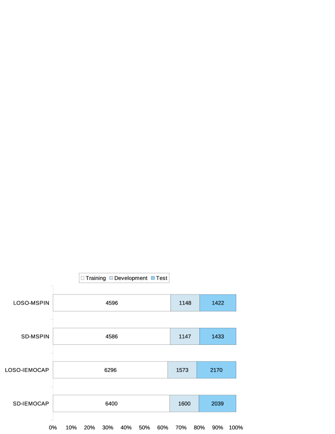
Figure 1: Proportions of data splitting for each partition of each dataset. In one-stage LSTM processing, the outputs of the model are both development and test data. In the second stage SVM processing, the input data is the prediction from the development set of the previous stage and the output is the prediction of test data.

3.2 Feature sets

Most research on SER, or generally on pattern classification, focuses on two main topics: feature extraction, as in Batliner et al. (2011), and classification/regression methods, as in Albornoz et al. (2011). While this research focuses on the second topic, we also evaluate state-of-the-art feature sets used for SER. For acoustic features, we evaluate three feature sets: the Geneva Minimalistic Acoustic Parameter Set (GeMAPS), statistical functions from GeMAPS, and the same functions from GeMAPS with a silence feature. For text features, aside from the original word vectors extracted from the text transcription, we also evaluate two word embeddings that are pretrained on a larger corpus: the Word2Vec embedding (Mikolov et al., 2013) and GloVe embedding (Pennington et al., 2014). These feature sets are explained below.

Acoustic features

The type of acoustic features extracted from a speech signal is the most important part of an SER system. GeMAPS is an effort to standardize the acoustic features used for voice research and affective computing (Eyben et al., 2016a). The feature set consists of 23 acoustic low-level descriptors (LLDs) such as fundamental frequency ($f_{0}$), jitter, shimmer, and formants, as listed in Table 1. As an extension of GeMAPS, eGeMAPS includes statistical functions derived from the LLDs, such as the minimum, maximum, mean, and other values. Since these features are extracted on frame-based processing, the feature size becomes large for one utterance (e.g., 3409 $\times$ 23 for IEMOCAP), which is suitable for deep learning methods like LSTM. Including the LLDs, the total number of features in eGeMAPS is 88. These statistical values are often called high-level statistical functions (HSF). Schmitt and Schuller (2018) found, however, that using only the mean and standard deviation (std) from the LLDs achieved a better result than using eGeMAPS and audiovisual features. These global features may represent more emotion information within speech than frame-based features. We thus coded these two statistical functions (47 values) from the LLDs as the HSF1 feature set. We also investigate the effect of including a silence feature in this SER research, as explained below. We define the combination of HSF1 with the silence feature as HSF2.

Silence, in this paper, is defined as the proportion of silent frames among all frames in an utterance. In human communication, the proportion of silence in speaking depends on the speaker’s emotion. For example, a happy speaker may have fewer silences (or pauses) than a sad speaker. The proportion of silence in an utterance can be calculated as

$$S=\frac{N_{s}}{N_{t}},$$ (1)

where $N_{s}$ is the number of frames categorized as silence (silent frames), and $N_{t}$ is the total number of frames. A frame is categorized as silent if it does not exceed a threshold value defined by multiplying a factor by a root mean square (RMS) energy, $X_{rms}$. Mathematically, this is formulated as

$$th=\alpha\times\overline{X_{rms}},$$ (2)

where $X_{rms}$ is defined as

$$X_{rms}=\sqrt{\frac{1}{n}\sum_{i=1}^{n}x[i]^{2}}.$$ (3)

This silence feature is similar to the disfluency feature proposed in Moore et al. (2014). In that paper, the author divided the total duration of disfluency by the total utterance length for $n$ words. Figure 2 illustrates the calculation of our silence feature. If $X_{rms}$ from a frame is below $th$, then it is categorized as silent, and the calculation of equation 1 is applied.

Table 1: Acoustic feature sets derived from the GeMAPS features by Eyben et al. (2016a) and the statistical functions used for dimensional SER in this research.

LLDs	HSF1	HSF2
intensity, alpha ratio, Hammarberg index, spectral slope 0-500 Hz, spectral slope 500-1500 Hz, spectral flux, 4 MFCCs, F0, jitter, shimmer, harmonics-to-noise ratio (HNR), harmonic difference H1-H2, harmonic difference H1-A3, F1, F1 bandwidth, F1 amplitude, F2, F2 amplitude, F3, and F3 amplitude.	mean (of LLDs), standard deviation (of LLDs)	mean (of LLDs), standard deviation (of LLDs), silence

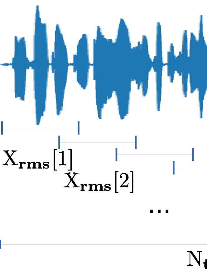
Figure 2: Moving frame to calculate the silence feature.

Text features

To process a word sequence in a computational model, the text must be converted to numerical values. The resulting text feature is commonly known as word embedding and is a vector representation of a word. Numerical values in the form of a vector are used to enable a computer to process text data, as it can only process numerical values. The values are points (numeric data) in a space whose number of dimensions is equal to the vocabulary size. The word representations embed those points in a feature space of lower dimension. In the original space, every word is represented by a one-hot vector, with a value of 1 for the corresponding word and 0 for other words. The element with a value of 1 is converted to a point in the range of the vocabulary size.

In addition to directly converting the text in the transcriptions of the datasets (IEMOCAP and MSP-I+N) to sequences, two pretrained word embeddings are used to weight the original word embeddings. As mentioned above, the two word-embedding models are Word2Vec (Mikolov et al., 2013) and GloVe (Pennington et al., 2014). Hence, we have three different text features for word embeddings: (1) a text sequence, or word embedding (WE), without any weighting, (2) a WE weighted by a pretrained Word2Vec model, and (3) a WE weighted by a pretrained GloVe embedding model. Word2Vec is trained on large datasets to model its vector representation by using either a continuous bag-of-words or a continuous skip-gram model. GloVe is another model to represent vector in words by analyzing linear direction by using a global log-bilinear regression method. All these features are fed into the same embedding layer in the text network.

4 Two-stage bimodal emotion recognition

4.1 Acoustic emotion recognition system

Most SER research uses only acoustic features. Our approach to acoustic SER is similar to that research. The contribution of our acoustic network is the evaluation of mean + std features at the utterance level and the use of a silence feature with the statistical functions to investigate any improvement. This evaluation is a continuation of (Tris Atmaja and Akagi, 2020) with extension on different feature sets and datasets. As explained in section 3.2, we evaluate three acoustic feature sets: LLDs, HSF1, and HSF2.

The LLD features are the 23 acoustic features listed in Table 1. For each frame (25 ms), these 23 acoustic features are extracted. With a hop size of 10 ms, the maximum number of sequences is 3409 for the IEMOCAP dataset and 3812 for the MSP-I+N dataset. Hence, the size of the input is 3409 $\times$ 23 for IEMOCAP and 3812 $\times$ 23 for MSP-I+N. The extraction process uses the openSMILE toolkit (Eyben et al., 2016b).

Figure 3 shows an overview of the acoustic network. LSTM is chosen because the number of training samples is adequate ($>5000$ samples) and it shows good results in the previous research (Schmitt and Schuller, 2018). Before entering the LSTM layers, the LLD features at the input layer are fed into a batch normalization layer to speed up the computation process. The three subsequent LSTM layers are stacked with 256 nodes in each layer, following one of the configurations in AbdelWahab and Busso (2018). Instead of returning the last output of the last LSTM layer, we designed the network to return the full sequence and flatten it before inputting it into three dense layers that represent valence, arousal, and dominance. The outputs of these last dense layers are then the predictions for those emotion attributes, i.e., the degrees of valence, arousal, and dominance in the range [-1, 1].

The tuning of hyper-parameters follows the previous research (Atmaja et al., 2019; Atmaja and Akagi, 2020). A batch size of 8 was used with a maximum of 50 epochs. An early stop criterion with ten patiences stops the training process if no improvement were made in 10 epochs (before the maximum epoch). The last highest-score model was used to predict the development data. An RMSprop optimizer was used with its default learning rate, i.e., $0.001$. Table 2 shows the setups on acoustic and text networks. These setups were obtained based on experiments with regard to the size of networks. For instance, the smaller acoustic networks with HSF features employed $\tanh$ output activation function and did not use the dropout rate, while the larger acoustic networks (with LLD) and text networks employed linear activation function and dropout rate.

Table 2: The hyper-parameter used in experiments

Hyper-parameter	Acoustic network	Text network
network type	LSTM	LSTM
number of layers	3	3
number of units	256	256
fourth layer	Flatten	Dense
hidden activation	linear	linear
output activation	linear (LLD) / tanh (HSF)	linear
dropout rate	0.3 (LLD) / 0 (HSF)	0.3
learning rate	0.001	0.001
batch size	8	8
maximum epochs	50	50
optimizer	RMSprop	RMSprop

For the HSF1 and HSF2 inputs on acoustic networks, the same setup applies. These two feature sets are very small as compared to the LLDs: HSF1 has a size of 1 $\times$ 46, while HSF2 has a size of 1 $\times$ 47. This big difference in input size (1:1800) leads to faster computation on HSF1 and HSF2 than on the LLDs. Note that although Figure 3 shows HSF2 as the input feature, the same architecture also applies to the LLDs and HSF1.

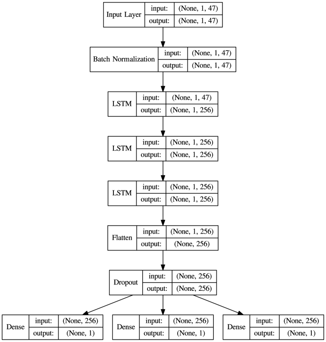
Figure 3: Structure of acoustic network to process acoustic features.

The idea of using LSTM is to hold the last output in memory and use that output as a successive step. For instance, LLD with ($3409,23$) feature size will process the first time step 1 to the last time step 3409. For HSF1 and HSF2, which contains a single time stamp, the data is processed only once ([1, 46] and [1, 47] for HSF1 and HSF2). Here, the only difference from multi-time steps is that the network performs three passes (forget gate, input gate, and output gate) instead of a single pass (see Eyben et al. (2010)). This information will include all information from the networks’ memory.

4.2 Text emotion recognition system

The text network, shown in Figure 4 for the MSP-I+N dataset, uses the same input size for the three different text features. The WE, WE with pretrained Word2Vec, and WE with pretrained GloVe embedding have 300 dimensions for each word. The longest sequence in the IEMOCAP dataset is 100 sequences (words), while for MSP-I+N, the longest is 300 sequences. Hence, the input feature sizes for the LSTM layers are 100 $\times$ 300 for IEMOCAP and 300 $\times$ 300 for MSP-I+N with its corresponding number of samples. The same three LSTM layers are stacked as in the acoustic network, but the last LSTM layer only returns the last output. A dense layer with a size of 128 nodes is added after the LSTM layers and before the last three dense layers. Between the dense layers is a dropout layer with the same probability of 0.3 to avoid overfitting.

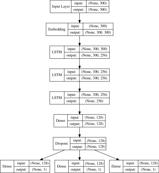
Figure 4: Structure of text network to process word embeddings/vectors.

4.3 Multitask learning

The task here in dimensional emotion recognition is to simultaneously predict the degrees of three emotion attributes, i.e., the degrees of valence, arousal, and dominance, for any given utterance. As the main target metric is the concordance correlation coefficient (CCC), the loss function is the CCC loss (CCCL). CCC also measures the performance of regression analyses by comparing gold standard labels and predictions. CCCL computes the score difference between the labels and predicted values for the three attributes. The CCC and CCCL are formulated as the following:

$$CCC =\dfrac{2\rho\sigma_{x}\sigma_{y}}{\sigma_{x}^{2}+\sigma_{y}^{2}+(\mu_{x}-\mu_{y})^{2}},$$ (4)

$$CCCL =1-CCC,$$ (5)

where $\rho$ is the Pearson correlation coefficient between the predicted emotion degree $x$ and the true emotion degree $y$, $\sigma^{2}$ is the variance, and $\mu$ is the mean. As the learning process minimizes three variables, we use the following multitask learning approach to optimize the CCC score:

$$CCCL_{tot}=\alpha CCCL_{V}+\beta CCCL_{A}+(1-\alpha-\beta)CCCL_{D},$$ (6)

where $\alpha$ and $\beta$ are respective CCCL parameters for valence (V) and arousal (A). The parameter for dominance (D) is obtained by subtracting $\alpha$ and $\beta$ from 1. The same parameter range [0, 1] with 0.1 steps is investigated for $\alpha$ and $\beta$ for both the acoustic and text networks, resulting in different optimal parameters, which are obtained by using linear search. Note that only positive values of $CCCL_{D}$’s parameters are used to investigate the optimal parameters.

4.4 SVM-based late fusion

We choose an SVM as the final classifier to fuse the outputs of the acoustic and text networks because of its effectiveness in handling smaller data (as compared to a DNN) and its computation speed. The datapoints produced by LSTM processing as the input of SVM are small; i.e., 1600, 1538, 1147, and 1148 for IEMOCAP-SD, IEMOCAP-LOSO, MSPIN-SD and MSPIN-LOS0, respectively. The SVM then applies a regression analysis to map them to the given labels. Figure 5 shows the architecture of this two-stage emotion recognition system using DNNs and an SVM. Each prediction from the acoustic and text networks is fed into the SVM. From two values (e.g., valence predictions from the acoustic and text networks), the SVM learns to generate a final predicted degree (e.g., for valence). The concept of using the SVM as the final classifier can be summarized as follows.

Suppose that two valence prediction outputs from the acoustic and text networks, $x_{i}=[x_{ser}[i],x_{ter}[i]]$, are generated by the DNNs, and that $y_{i}$ is the corresponding valence label. The problem in dimensional SER fusing acoustic and text results is to minimize the following:

$$\underset{w,b,\zeta,\zeta^{*}}{\text{min}} \frac{1}{2}w^{T}w+C\sum_{i=1}^{n}\zeta_{i}+C\sum_{i=1}^{n}\zeta_{i}^{*}$$ (7)

subject to $$w^{T}\phi(x_{i})+b-y_{i}\leq\epsilon+\zeta_{i},$$

$$y_{i}-w^{T}\phi(x_{i})-b\leq\epsilon+\zeta_{i}^{*},$$

$$\zeta_{i},\zeta_{i}^{*}\geq 0,i=1,\ldots,n,$$

where $w$ is a weighting vector, $C$ is a penalty parameter, $\zeta$ and $\zeta^{*}$ is the distance between misclassified points and the corresponding marginal boundary (above or below). Here, $\phi$ is the kernel function. We choose a radial basis function (RBF) kernel because of its flexibility in modeling a nonlinear process with a dimensional emotion model close to this kernel. The function $\phi$ for the RBF kernel is formulated as

$$K(x_{i},x_{j})=e^{\gamma(x_{i}-x_{j})^{2}},$$ (8)

where $\gamma$ defines how much influence a single training has on the model. All parameters in this SVM are obtained empirically via linear search in a specific range. Although the explanation above uses valence, the same also applies for arousal and dominance.

Figure 5: Proposed two-stage dimensional emotion recognition method using DNNs and an SVM. The inputs are acoustic features (af) and text features (tf); the outputs are valence (v), arousal (a), and dominance (d).

4.5 Reproducibility

The experimental code was written in Python, and, for the sake of research reproducibility, it is available in the following repository: https://github.com/bagustris/two-stage-ser. The DNN part was implemented using Keras by Chollet and Others (2015) and Tensorflow, while the SVM-based fusion was implemented using the scikit-learn toolkit by Pedregosa et al. (2011). To obtain consistent results for each run, some fixed numbers are initialized at the beginning, as can be found in the repository above.

5 Results and discussions

5.1 Results from single modality

Before presenting the bimodal feature-fusion results, it is important to show the results of unimodal emotion recognition. The goals here are (1) to observe the (relative) improvement of bimodal feature fusion over using a single modality, and (2) to observe the effects of different features on different emotion attributes.

Tables 3 and 4 list the single-modality results of dimensional emotion recognition from the acoustic and text networks, respectively. In general, acoustic-based SER gave better results than text-based SER in terms of the average CCC score. For particular emotion attributes, the text network gave a higher CCC score for valence prediction than those obtained by the acoustic network, except on the MSPIN datasets. This confirms the previous finding by Karadogan and Larsen (2012) that valence is better estimated by semantic features, while arousal is better predicted by acoustic features. In addition, we found that the dominance dimension was better predicted by acoustic features than by text features. This finding can be inferred from both tables, in which the CCC scores for the dominance dimension are frequently higher from the acoustic network than from the text network.

The exception of a higher valence score on the MSPIN-SD dataset by the acoustic network can be seen as the effect of either the DNN architecture or the dataset’s characteristics. In Chen et al. (2017), the obtained score was higher for valence than for arousal or liking (the third dimension, instead of dominance) with their strategy on acoustic features. In contrast, AbdelWahab and Busso (2018) obtained a lower score for valence than for arousal and dominance by using their proposed DANN method on the same MSP-IMPROV dataset (whole data, all four scenarios). Given this comparison, we conclude that the higher valence score obtained here was an effect of the DNN architecture because of the multitask learning. Our result on a single modality (acoustic network) outperformed the DANN result on MSP-IMPROV, where their highest CCC scores were (0.303, 0.176, 0.476) as compared to our scores of (0.404, 0.605, 0.517) for valence, arousal, and dominance, respectively.

Table 3: CCC score results of dimensional emotion recognition using an acoustic network. The best results on the test set are in bold. LLDs: low-level descriptors from GeMAPS (Eyben et al., 2016a); HSF1: mean + std of LLDs; HSF2: mean + std + silence.

Feature set	V	A	D	Mean
IEMOCAP-SD
LLD	0.153	0.522	0.534	0.403
HSF1	0.186	0.535	0.466	0.396
HSF2	0.192	0.539	0.469	0.400
MSPIN-SD
LLD	0.299	0.545	0.441	0.428
HSF1	0.400	0.603	0.506	0.503
HSF2	0.404	0.605	0.517	0.508
IEMOCAP-LOSO
LLD	0.168	0.486	0.442	0.365
HSF1	0.206	0.526	0.442	0.391
HSF2	0.204	0.543	0.442	0.396
MSPIN-LOSO
LLD	0.176	0.454	0.369	0.333
HSF1	0.201	0.506	0.357	0.355
HSF2	0.206	0.503	0.346	0.352

Table 4: CCC score results of dimensional emotion recognition using text networks; each score is an averaged score of 20 runs with its standard deviation. WE: word embedding; Word2Vec: WE weighted by pretrained word vector (Mikolov et al., 2013); GloVe: WE weighted by pretrained global vector (Pennington et al., 2014).

Feature set	V	A	D	Mean
IEMOCAP-SD
WE	0.389 $\pm$ 0.008	0.373 $\pm$ 0.010	0.398 $\pm$ 0.017	0.387 $\pm$ 0.010
Word2Vec	0.393 $\pm$ 0.012	0.371 $\pm$ 0.018	0.366 $\pm$ 0.024	0.377 $\pm$ 0.016
GloVe	0.410 $\pm$ 0.007	0.381 $\pm$ 0.013	0.393 $\pm$ 0.016	0.395 $\pm$ 0.010
MSPIN-SD
WE	0.120 $\pm$ 0.047	0.148 $\pm$ 0.023	0.084 $\pm$ 0.024	0.105 $\pm$ 0.026
Word2Vec	0.138 $\pm$ 0.031	0.108 $\pm$ 0.024	0.101 $\pm$ 0.024	0.116 $\pm$ 0.017
GloVe	0.147 $\pm$ 0.043	0.141 $\pm$ 0.019	0.098 $\pm$ 0.017	0.128 $\pm$ 0.015
IEMOCAP-LOSO
WE	0.376 $\pm$ 0.008	0.359 $\pm$ 0.018	0.370 $\pm$ 0.020	0.368 $\pm$ 0.013
Word2Vec	0.375 $\pm$ 0.058	0.357 $\pm$ 0.058	0.365 $\pm$ 0.065	0.366 $\pm$ 0.059
GloVe	0.405 $\pm$ 0.009	0.382 $\pm$ 0.020	0.378 $\pm$ 0.021	0.389 $\pm$ 0.014
MSPIN-LOSO
WE	0.076 $\pm$ 0.013	0.196 $\pm$ 0.011	0.136 $\pm$ 0.015	0.136 $\pm$ 0.009
Word2Vec	0.162 $\pm$ 0.008	0.202 $\pm$ 0.005	0.147 $\pm$ 0.003	0.170 $\pm$ 0.000
GloVe	0.192 $\pm$ 0.004	0.189 $\pm$ 0.007	0.129 $\pm$ 0.004	0.170 $\pm$ 0.003

To find the optimal parameter values for $\alpha$ and $\beta$, a linear search was performed on the scale [0.0, 1.0] with a step of 0.1. Using this conventional technique, we found four sets of optimal parameters for the acoustic and text networks. Note that while only the improvised and natural scenarios (MSP-I+N) were used to find the optimal text-network parameters for the MSP-IMPROV dataset, the whole dataset was used to find the optimal acoustic-network parameters. Table 5 lists the optimal parameter values for $\alpha$ and $\beta$.

Table 5: Optimal parameters for multitask learning.

Dataset	Modality	$\alpha$	$\beta$
IEMOCAP	acoustic	0.1	0.5
	text	0.7	0.2
MSP-IMPROV	acoustic	0.3	0.6
	text	0.1	0.6

To summarize the single-modality results, average CCC scores from three emotion dimensions can be used to justify which features perform better among others. The results show that HSF2 was the most useful of the acoustic feature sets (in two of four datasets), while the word embedding (WE) with pretrained GloVe embedding was the most useful of the text feature sets. The performance of dimensional emotion recognition in the speaker-independent (LOSO) case was lower than in the speaker-dependent (SD) case, as predicted. Note that both acoustic and text emotion networks used a fixed seed number to achieve the same result for each run; however, the text network resulted in different scores. Hence, standard deviations were given to measure fluctuation in 20 runs.

5.2 Results from SVM-based fusion

The main proposal of this research is the late-fusion approach combining the results from acoustic and text networks for dimensional emotion recognition. This subsection presents the results of the late-fusion approach, including the obtained performances, comparison with the single-modality results, which pairs of acoustic-text results performed better, and our overall findings.

For each dataset (IEMOCAP-SD, MSPIN-SD, IEMOCAP-LOSO, MSPIN-LOSO), nine combinations of acoustic-text result pairs could be fed to the SVM system. Tables 6, 7, 8, and 9 list the respective CCC results for these datasets. Generally, our proposed two-stage dimensional emotion recognition improved the CCC score from single-modality emotion recognition. The pair of results from HSF2 (acoustic) and Word2Vec (text) gave the highest CCC score on speaker-dependent scenarios.

On the speaker-independent IEMOCAP dataset (IEMOCAP-LOSO), the result from the pair of HSF2 and GloVe gave the highest CCC score. This result linearly correlated with the single-modality results for that dataset, in which HSF2 obtained the highest CCC score among the acoustic features, and GloVe was the best among the text features. On the four datasets, the results from HSF2 obtained the highest CCC score for two out of four datasets, while GloVe obtained the highest CCC score for all four datasets. Hence, we conclude that the highest result from a single modality, when paired with the highest result from another modality, will achieve the highest performance among possible pairs.

Table 6: CCC score results after late fusion using an SVM on the IEMOCAP-SD test set.

Inputs	V	A	D	Mean
LLD + WE	0.520	0.602	0.519	0.547
LLD + Word2Vec	0.552	0.613	0.524	0.563
LLD + GloVe	0.546	0.606	0.520	0.557
HSF1 + WE	0.578	0.575	0.490	0.548
HSF1 + Word2Vec	0.599	0.590	0.491	0.560
HSF1 + GloVe	0.595	0.582	0.495	0.557
HSF2 + WE	0.598	0.591	0.502	0.564
HSF2 + Word2Vec	0.595	0.601	0.499	0.565
HSF2 + GloVe	0.598	0.591	0.502	0.564

Table 7: CCC score results after late fusion using an SVM on the MSPIN-SD dataset.

Inputs	V	A	D	Mean
LLD + WE	0.344	0.591	0.447	0.461
LLD + Word2Vec	0.326	0.586	0.439	0.450
LLD + GloVe	0.344	0.585	0.439	0.456
HSF1 + WE	0.461	0.637	0.517	0.538
HSF1 + Word2Vec	0.464	0.634	0.518	0.539
HSF1 + GloVe	0.466	0.630	0.510	0.535
HSF2 + WE	0.475	0.640	0.522	0.546
HSF2 + Word2Vec	0.486	0.641	0.524	0.550
HSF2 + GloVe	0.485	0.638	0.523	0.549

Table 8: CCC score results after late fusion using an SVM on the IEMOCAP-LOSO test set.

Inputs	V	A	D	Mean
LLD + WE	0.537	0.583	0.431	0.517
LLD + Word2Vec	0.528	0.580	0.421	0.510
LLD + GloVe	0.539	0.587	0.430	0.518
HSF1 + WE	0.565	0.565	0.453	0.528
HSF1 + Word2Vec	0.536	0.559	0.434	0.510
HSF1 + GloVe	0.559	0.570	0.452	0.527
HSF2 + WE	0.524	0.566	0.452	0.514
HSF2 + Word2Vec	0.531	0.571	0.445	0.516
HSF2 + GloVe	0.553	0.579	0.465	0.532

Table 9: CCC score results after late fusion using an SVM on the MSPIN-LOSO test set.

Inputs	V	A	D	Mean
LLD + WE	0.204	0.485	0.387	0.358
LLD + Word2Vec	0.267	0.487	0.386	0.380
LLD + GloVe	0.269	0.482	0.375	0.376
HSF1 + WE	0.224	0.565	0.410	0.400
HSF1 + Word2Vec	0.286	0.558	0.411	0.418
HSF1 + GloVe	0.282	0.555	0.409	0.415
HSF2 + WE	0.232	0.566	0.421	0.406
HSF2 + Word2Vec	0.287	0.562	0.411	0.420
HSF2 + GloVe	0.291	0.570	0.405	0.422

To evaluate the improvement obtained by SVM-based late fusion, the average CCC scores again can be used as a single metric. The rightmost column in Tables 6, 7, 8, and 9 shows the average CCC scores obtained from the nine pairs of acoustic and text results on the four different datasets. Comparing these bimodal results to unimodal results (Table 3 and 4) shows the difference. All results from SVM improved unimodal results. In speaker-independent (LOSO) results (which are more appropriate for real-life analysis), the scores resulted by pairs of HSF with any word vector obtain remarkable improvements, particularly in the MSPIN-LOSO dataset. For any other pair involving LLDs, the obtained score was also lower as compared to other pairs. Considering all low scores involved LLD results, improving the performance of dimensional emotion recognition by using LLDs is more complicated than by using HSF1 and HSF2, apart from the larger feature size and the longer training time. The large network size created by an LLD input as a result of its much bigger feature dimension (e.g., 3409 $\times$ 23 on IEMOCAP) did not help either the single-modality or late-fusion performance. In contrast, the small sizes of the functional features (HSF1 and HSF2) enabled better performance on a single modality, which led to better performance for the late-fusion score. To obtain functional features, however, a set of LLD features must be obtained first. This problem is a challenging future research direction, especially for implementing dimensional emotion recognition with real-time processing.

Aside from the fact that a speaker-independent dataset is usually more difficult than a speaker-dependent dataset, the low score on MSPIN-LOSO was due to its low scores on a single modality. In other words, lower pair performance from a single modality will result in low performance in late fusion. In particular, these low results derive from low CCC scores from the text modality (Table 4). The average CCC score for the text modality on the MSPIN-LOSO dataset was less than 0.16, compared to an average score higher than 0.34 for the acoustic modality. All nine pairs in late-fusion approaches improved on the single-modality results because of the two-stage DNN and SVM regression analysis. Thus, out of 36 trials (9 pairs $\times$ 4 datasets), our proposed two-stage dimensional emotion recognition outperforms any single modality result (used in a pair).

The low score on MSPIN for the text modality can be tracked to the origin of the dataset; that is, there may have been a number of sentences semantically identical to the target sentences in the dataset we used. Although we chose sentences only from the improvised dialogues (minus the target sentence) and from the natural interactions (those sentences produced by the experimenters and subjects during the breaks), some of the sentences in this corpus were semantically identical to that of the target sentences in the “Target-Improvised” data set. This was confirmed retroactively by manually checking the provided transcription and our automatic transcription. Given the nature of the elicitation task in a dialogue framework, this is not surprising. A similarly low result for the text modality on this MSPIN dataset was also shown in Zhang et al. (2019). In general, compared to the IEMOCAP dataset, the MSPIN dataset suffers from low accuracy in recognizing the valence category by using acoustic and lexical properties. Interestingly, however, those authors also did not show improvement on the IEMOCAP scripted dataset, another text-based session in which lexical/text features do not contribute significantly.

To measure the improvement by our proposed two-stage late fusion, we calculated the relative improvement obtained by late fusion from the highest CCC scores for a single modality. For example, the pair of LLD + WE used the results from the LLDs in the acoustic network and the WE in the text network. We compared the result for LLD + WE with that for the LLDs, as it had a higher score than the WE did. Figure 6 thus shows the relative improvement for all nine pairs. All of 36 trials showed improvements ranging from 5.11% to 40.32%. Table 10 lists the statistics for the obtained relative improvement. Our results show higher relative accuracy improvement as compared to those obtained by Zhang et al. (2019) for valence prediction, which ranged from 6% to 9%. Nevertheless, their multistage fusion method also showed benefits over the multimodal and single-modality approaches. These findings confirm the benefits of using bimodal/multimodal fusion instead of single-modality processing for valence, arousal, and dominance prediction.

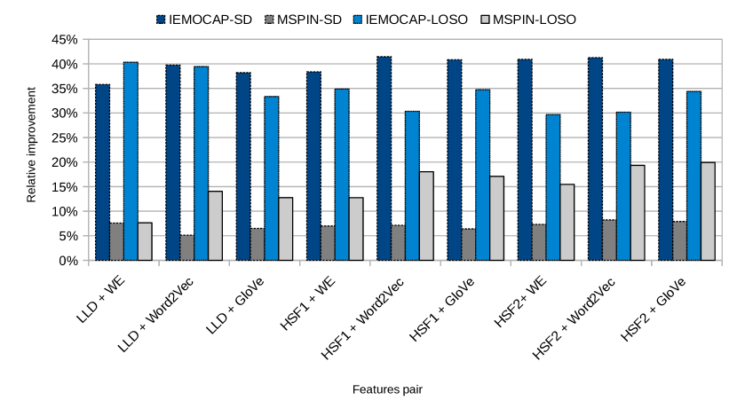
Figure 6: Relative improvement in average CCC scores from late fusion using an SVM as compared to the highest average CCC scores from a single modality.

Table 10: Statistics of relative improvement by late fusion using an SVM as compared to the highest scores for a single modality across datasets; the scores were extracted from the data shown in Figure 6.

Statistic	IEMOCAP-SD	MSPIN-SD	IEMOCAP-LOSO	MSPIN-LOSO
Average	39.73%	7.01%	34.15%	15.23%
Max	41.45%	8.22%	40.32%	19.93%
Min	35.80%	5.11%	29.69%	7.64%
Std	1.90%	0.93%	3.84%	3.90%

5.3 Speaker-dependent vs. speaker-independent text emotion recognition

While speech-based emotion recognition is performed with a fixed random seed to generate the same result for each run, text-based emotion recognition results in different scores for each run. The different results on text emotion recognition probably were caused by the initiation of weightings on embedding layers. In this case, statistical tests can be performed on text emotion results to observe the difference between speaker-dependent and speaker-independent scenario. In contrast, statistical tests cannot be performed between acoustic results and bimodal acoustic-text results due to differences in the data (deterministic vs. non-deterministic).

Table 11 shows if there is a significant difference between speaker-dependent and speaker-independent results on the same feature set. We set $p-$value = 0.05 with a two-tail paired t-test between mean scores of speaker-dependent and speaker-independent results. This paired t-test was based on the assumption that there are no outliers (after pre-processing) and two different inputs are fed into the same system. Only one result from text emotion recognition shows no significant difference on IEMOCAP dataset while all results on MSPIN dataset show a significant difference between speaker-dependent and speaker-independent results. This result reveals a tendency for a difference in evaluating speaker-dependent and speaker-independent data. The results from speaker-dependent data were different from those of speaker-independent data. In other words, results from speaker-dependent data cannot be used to justify speaker-independent or whole data.

Table 11: Significant difference between speaker-dependent and speaker-independent scenario on the same text feature set; statistical tests were performed using two-tail paired $t-$test with $p-$value = 0.005.

Feature	IEMOCAP	MSPIN
WE	Yes	Yes
Word2Vec	No	Yes
GloVe	Yes	Yes

5.4 Effect of removing target sentence from MSPIN dataset

Since the goal of this research is to evaluate the contribution of both acoustic and linguistic information in affective expressions, it is necessary to have sentences in the dataset that are free from any stimuli control. However, the original MSP-IMPROV dataset contains 20 “target” sentences; a sentence with the same linguistic content but produced with different emotions. These parts of MSP-IMPROV dataset are irrelevant to this study; hence, we remove it from the dataset (Target - improvised and Target - read parts). However, we found that the results show low CCC scores (Table 4, particularly on valence) indicating influence from target sentences. These results may be explained, as mentioned in section 5.2, that some utterances in the data analyzed in this study also inadvertently included sentences semantically the same as those in the improvised target sentences.

5.5 Final remarks

We tried to perform a benchmark between our results and others on the same datasets, scenarios, and metrics. Unfortunately, to the best of our knowledge, the only reference is the one reported by Atmaja and Akagi (2020), which reports an early fusion method on IEMOCAP dataset. We improve the average CCC score from $0.508$ to $0.532$. This higher result suggests that late fusion is better than early fusion in modeling how humans fuse multimodal information, which is in line with neuropsychological research. This late-fusion approach can be embedded with current speech technology, i.e., ASR, in which the text output can be processed to weigh emotion prediction from acoustic features.

AbdelWahab and Busso (2018) used MSP-Podcast (Lotfian and Busso, 2019) as a target corpora, which is not available for the public yet, and IEMOCAP with MSP-IMPROV as a source corpus to implement their DANN for cross-corpus speech emotion recognition. Although the goal is different, we observed similar patterns between theirs and our acoustic-only speech emotion recognition. First, we observed that the order of highest to lowest CCC scores is arousal, dominance, and valence. This pattern is also consistent when IEMOCAP is mixed with MSP-IMPROV as reported by Parthasarathy and Busso (2017) (in Table 2). Second, we observed that the CCC scores obtained in IEMOCAP are higher than those obtained in MSP-IMPROV; we believe that this lower score in MSP-IMPROV was due to the smaller size of the dataset.

Along with our SVM architecture, we also explored the parameters $C$ and $\gamma$, because both parameters are important for an RBF-kernel-based SVM architecture (Pedregosa et al., 2011). Linear search was used in the ranges of [$10^{-2},1,10^{2},2\times 10^{2},3\times 10^{2}$] for $C$ and [$10^{-2},10^{-1},1,10,10^{2}$] for $\gamma$ with a fixed value of $\epsilon$, i.e., 0.01. The best parameter values were $C=200$ and $\gamma=0.1$. The repository includes the detailed implementation of the SVM architecture.

Per our stated objective, we applied two-stage processing by using DNNs and an SVM for dimensional emotion recognition from acoustic and text features on four different datasets. We found that the combination of mean + std + silence from the acoustic features and word embeddings weighted by pretrained GloVe embeddings achieved the highest result among the nine pairs of acoustic-text results from DNNs trained with multitask learning. When the performance in obtaining one input to the SVM is very low, the resulting relative improvement due to the SVM is also low. For instance, the lowest improvement on MSPIN-LOSO was from LLD + WE features, in which WE obtained a low score ($\overline{CCC}=0.136$) on text network. This phenomenon suggests a challenging future research direction for dealing with minimal linguistic information in the fusion strategy. One strategy applied in this research was to use a pretrained GloVe embedding on text features with HSF2 on acoustic features, which improved the $\overline{CCC}$ score from 0.358 (relative improvement = 7.64%) to 0.422 (relative improvement = 19.93%). Other strategies should also be proposed, such as how to handle the data differently when the linguistically identical sentences elicit different emotions (i.e., the whole MSP-IMPROV dataset). In contrast, the currently evaluated word embeddings treat the same words to have the same representations, even when it conveys different emotions.

6 Conclusions

In conclusion, we summarize several findings. First, we found a linear correlation between the single-modality and late-fusion methods in dimensional emotion recognition. The best results from each modality, when they were paired, gave the best fusion result. In the same way, the worst results obtained from each network, when they were paired, gave the worst fusion results for bimodal emotion recognition. This finding differs from that reported in Atmaja et al. (2019), which used an early-fusion approach for categorical emotion recognition. In their work, the best pair differs from the best methods in single modalities.

Second, text features strongly influenced the score of dimensional SER on the valence dimension, while acoustic features strongly influenced arousal and dominance scores. Accordingly, the proposed two-stage processing can take advantage of text features that are commonly used in predicting sentiment (valence) for the dimensional emotion recognition task. The proposed fusion method improves all three emotion dimensions without attenuating the performance of any dimension. That is, the proposed method elevates the scores for valence, arousal, and dominance subsequently from the highest to the lowest gain.

Third, the combination of input pairs does not matter in the proposed fusion method, as indicated by the low deviation in relative improvement across the nine possible input pairs. What does matter is the performance of the input in the DNN stage. If the performance of a feature set in the DNN stage is low ($\overline{CCC}\leq 0.2$), it will also result in low performance when paired with another low-performance input in the SVM stage.

Finally, this bimodal approach can be extended to a multimodal approach. Both acoustic and text features can be combined with visual and motion-capture measurements that have advantages in specific emotion dimensions (liking or naturalness). The results can be benchmarked with current results to observe such improvements by adding more modalities. The SVM stage itself can be performed many times to obtain such improvements. These broad research directions are open challenges for researchers in human-computer interaction.