Imputation of missing values in multi-view data

Abstract

Data for which a set of objects is described by multiple distinct feature sets (called views) is known as multi-view data. When missing values occur in multi-view data, all features in a view are likely to be missing simultaneously. This leads to very large quantities of missing data which, especially when combined with high-dimensionality, makes the application of conditional imputation methods computationally infeasible. We introduce a new imputation method based on the existing stacked penalized logistic regression (StaPLR) algorithm for multi-view learning. It performs imputation in a dimension-reduced space to address computational challenges inherent to the multi-view context. We compare the performance of the new imputation method with several existing imputation algorithms in simulated data sets. The results show that the new imputation method leads to competitive results at a much lower computational cost, and makes the use of advanced imputation algorithms such as missForest and predictive mean matching possible in settings where they would otherwise be computationally infeasible.

keywords missing data, imputation, multi-view learning, stacked generalization, feature selection

1 Introduction

Multi-view data refers to any data set where the features have been divided into distinct feature sets [1, 2]. Such data sets are particularly common in the biomedical domain where these feature sets, commonly called views, often correspond to different data sources or modalities [3, 4, 5, 6]. Classification models of disease using information from multiple views generally lead to better performance than models using only a single view [7, 8, 9, 10, 11, 12]. Traditionally, information from different views is often combined using simple feature concatenation, where the features corresponding to different views are simply aggregated into a single feature matrix, so that traditional machine learning methods can be deployed [3]. More recently, dedicated multi-view machine learning techniques have been developed, which are specifically designed to handle the multi-view structure of the data [2, 3]. One such multi-view learning technique is stacked penalized logistic regression (StaPLR) [13]. In addition to improving classification performance, StaPLR can automatically select the views most relevant for prediction [13, 14, 15].

In practice, not all views may be observed for all subjects. When confronted with missing views, typical approaches are to remove any subjects with at least one missing value from the data set (called list-wise deletion or complete case analysis (CCA)), or to replace missing values by some substituted value, a process known as imputation. In biomedical studies, a single view may consist of thousands or even millions of features. With the traditional approach of feature concatenation, in the presence of missing views, CCA leads to a massive loss of information, while imputation may be computationally infeasible. In this article we propose a new method for dealing with missing views, based on the StaPLR algorithm. We show how this method requires much less computation by imputing missing values in a dimension-reduced space, rather than in the original feature space. We compare our proposed meta-level imputation method with imputation methods applied in the original feature space.

2 Methods

Missing values are often divided into three categories: missing completely at random (MCAR), missing at random (MAR), or missing not at random (MNAR) [16, 17]. Values are said to be MCAR if the causes of the missingness are unrelated to both missing and observed data [17]. Examples include random machine failure, or missingness introduced by analyzing a random sub-sample of the data. If the missingness is not completely random but depends only on observed data, the missing values are said to be MAR [17]. If the missingness instead depends on unobserved factors, the missing values are said to be MNAR [17]. Here, we will focus on MCAR missing values.

The simplest way of dealing with MCAR missing values is to discard observations with at least one missing value through complete case analysis. However, this approach is potentially very wasteful since a single missing value causes an entire observation to be removed from the data. CCA may therefore remove many more observed values from the data than the number of values initially missing, and drastically reduce the sample size, leading to increased variance and therefore less accurate predictions.

To prevent wasting observed data, missing values can be imputed. The simplest form of imputation is to simply replace each missing value by the unconditional mean of the feature, a procedure known as (unconditional) mean imputation (MI). If one is primarily interested in prediction, MI has some favorable properties: Its computational cost is extremely small, and it has been shown that MI is universally consistent for prediction even for MAR data, as long as the learning algorithm used is also universally consistent [18]. Here consistent means that, given an infinite amount of training data, the prediction function achieves the error rate of the best possible prediction function (i.e. the Bayes rate), while universal means that the procedure is consistent for all possible data distributions [18]. However, MI is often criticised because it is known to distort the data distribution by attenuating existing correlations between the features, underestimating the variance, and causing bias in almost any estimate other than the mean [17]. More sophisticated imputation methods include Bayesian linear regression, predictive mean matching (PMM) [17], and missForest (MF) [19]. These methods are multiple imputation methods, meaning multiple imputed data sets are formed so that correct variance estimates can be obtained [17].

It should be noted that other methods for handling missing data exist which do not explicitly impute missing values. These methods incorporate the missing data handling directly into the model fitting procedure and include likelihood-based methods such as full information maximum likelihood (FIML) [20, 21] for parametric regression models, and missingness incorporated in attributes (MIA) [22] for decision trees. However, these methods are less broadly applicable than imputation methods [21, 17, 18] and we do not consider them here.

The literature on the imputation of missing values is vast, and we do not aim to give a complete overview here. Instead, we divide the existing imputation methods in two broad classes: unconditional and conditional imputation. We define an unconditional imputation method as any method in which the imputation of a missing value is based solely on other observations of the same feature, that is, the imputation takes place within a single column of the feature matrix. The aforementioned mean imputation is a classical example of an unconditional imputation method. By contrast, a conditional imputation method is any method in which the imputation of a missing value is based, in part or completely, on observations of other features, that is, the imputation uses different columns of the feature matrix. Most sophisticated imputation methods, such as Bayesian multiple imputation and PMM, are conditional imputation methods. The distinction between unconditional and conditional imputation methods is of particular interest for feature selection. Unconditional imputation methods, such as mean substitution, use only the univariate distributions for imputation, so that the imputed feature remains in some sense “pure” and free from contamination from other features. However, as mentioned earlier, mean substitution is known to distort the data distribution by attenuating existing correlations between the features [17].

By contrast, some (but not all) conditional imputation methods preserve the correlations between features [17]. However, in this case the imputed values depend on other features in the data. In the event that a selected feature has a large number of imputed values, this may lead to difficulties in interpretation, since a large proportion of the selected feature is derived from other features. Nevertheless, a recent study on the effect of imputation methods on feature selection suggests sophisticated conditional imputation methods generally lead to better results than unconditional imputation [23]. Because it is not possible to both perform the imputation independent of other features and preserve the existing correlations, one has to choose between one or the other.

2.1 From Missing Features to Missing Views

In multi-view data, it is likely that missingness will occur at the view level, rather than at the feature level. Missing views may occur at random and/or by design. In a study where one of the views corresponds to features derived from a magnetic resonance imaging (MRI) scan, factors like the MRI scanner experiencing machine failure, a mistake in the scanning protocol by the researcher administering the scan, or a subject simply not making it to their appointment in time due to heavy traffic, would lead to all features of this view being simultaneously missing. Likewise, if one of the views corresponds to features derived from a sample of blood or cerebral spinal fluid (CSF), a lost or contaminated sample would lead to all derived features being simultaneously missing. Note that in these cases, although the missingness occurs at the view level, the underlying mechanism is still MCAR. Another common example of MCAR data occurs in the case of planned missingness, where the missing values are part of the study design. For example, it may be considered too expensive to administer an MRI scan to all study participants, so instead an MRI scan is administered only to a random sub-sample of the participants. Again the underlying mechanism is MCAR, but all features corresponding to the MRI scan will be missing simultaneously for the unmeasured sub-sample. Throughout the rest of this article we will assume that (1) for each observation, a view is either completely missing or completely observed, and (2) the missingness is completely at random (MCAR).

Conceptually, one could impute a missing view by first applying feature concatenation, and then simply applying a chosen imputation method on the concatenated feature set. However, in practice this may be impossible. For example, if the missing view is an MRI scan, there could be hundreds of thousands or even millions of missing values. Similar numbers of missing values may occur with views corresponding to other neuroimaging techniques, gene-expression arrays, or other omics-data. With such vast amounts of missing values, application of sophisticated multiple-imputation methods may be computationally infeasible. For example, multiple imputation by chained equations, a very popular method for handling missing data implemented in the R package mice [24] involves iteratively cycling through a procedure of model-fitting and generating imputed values from the fitted model. Such iterative approaches quickly become prohibitive with large numbers of predictor variables, where the computational load of even a single imputation will exceed that of fitting the final predictive model of interest. This process is further complicated by the small sample sizes and thus extreme high-dimensionality commonly seen in neuroimaging, which means that even in instances where the imputation would be computationally feasible, the obtained results may be of poor quality (see Appendix A for further explanation). However, by analyzing the multi-view data using the StaPLR algorithm, we will introduce a method of dealing with the missing views in a much less computationally intensive way.

2.2 The StaPLR Algorithm

The general StaPLR algorithm was proposed by van Loon et al. [13], and later extended to more than 2 levels of stacking [15]. For clarity, we will assume throughout this article that (1) there are only 2 levels of stacking, the base (feature) level, and the meta (view) level, and (2) there is only one base learning algorithm ($A_{\text{b}}$), which is the same for all views. Under these assumptions the StaPLR algorithm can be given by Algorithm 1, and displayed as a flow diagram as in Figure 1. For each view $\bm{X}^{(v)},v=1\dots V$, a trained classifier $\hat{f}_{v}$ is obtained by applying the base-learning algorithm $A_{\text{b}}$ to the pair $\bm{X}^{(v)},\bm{y}$. In our case $A_{\text{b}}$ is an $L_{2}$-penalized logistic regression learner including cross-validation for the tuning parameter, so that each $\hat{f}_{v}$ is a fully tuned logistic ridge regression classifier. For each of the base-classifiers $\hat{f}_{v},v=1\dots V$, $k$-fold cross-validation is performed to obtain a vector $\bm{z}^{(v)}$ of estimated out-of-sample predictions. These predictions take the form of predicted probabilities rather than hard class labels. The vectors $\bm{z}^{(v)},v=1\dots V$, are concatenated column-wise into the matrix $\bm{Z}$, which is then used together with outcome $\bm{y}$ to train the meta-learning algorithm $A_{\text{m}}$ and obtain the meta-classifier $\hat{f}_{\text{meta}}$. In our case, $A_{\text{m}}$ is an $L_{1}$-penalized nonnegative logistic regression learner including cross-validation for the tuning parameter, so that $\hat{f}_{\text{meta}}$ is a fully tuned logistic nonnegative lasso classifier. The final classifier is then given by $\hat{f}_{\text{stacked}}=\hat{f}_{\text{meta}}\circ(\hat{f}_{\text{1}}\dots\hat{f}_{\text{V}})$.

Data: Views $\bm{X}^{(1)},\dots,\bm{X}^{(V)}$ and outcomes $\bm{y}=(y_{1},\dots,y_{n})^{T}$.

1 foreach $v$ = 1 to $V$ do

2       $\hat{f}_{v}=A_{\text{b}}(\bm{X}^{(v)},\bm{y})$

3       foreach $k$ = 1 to $K$ do

4             $\hat{f}_{v,k}=A_{\text{b}}(\bm{X}^{(v)}_{i\notin S_{k}},\bm{y}_{i\notin S_{k}})$

5             $\bm{z}^{(v)}_{k}=\hat{f}_{v,k}(\bm{X}^{(v)}_{i\in S_{k}})$

6       end foreach

7      

8 end foreach

9$\bm{Z}=(\bm{z}^{(1)},\dots,\bm{z}^{(V)})$

10 $\hat{f}_{\text{meta}}=A_{\text{m}}(\bm{Z},\bm{y})$

$\hat{f}_{\text{stacked}}=\hat{f}_{\text{meta}}\circ(\hat{f}_{\text{1}}\dots\hat{f}_{\text{V}})$

Algorithm 1 The 2-level StaPLR algorithm, with a single base learner

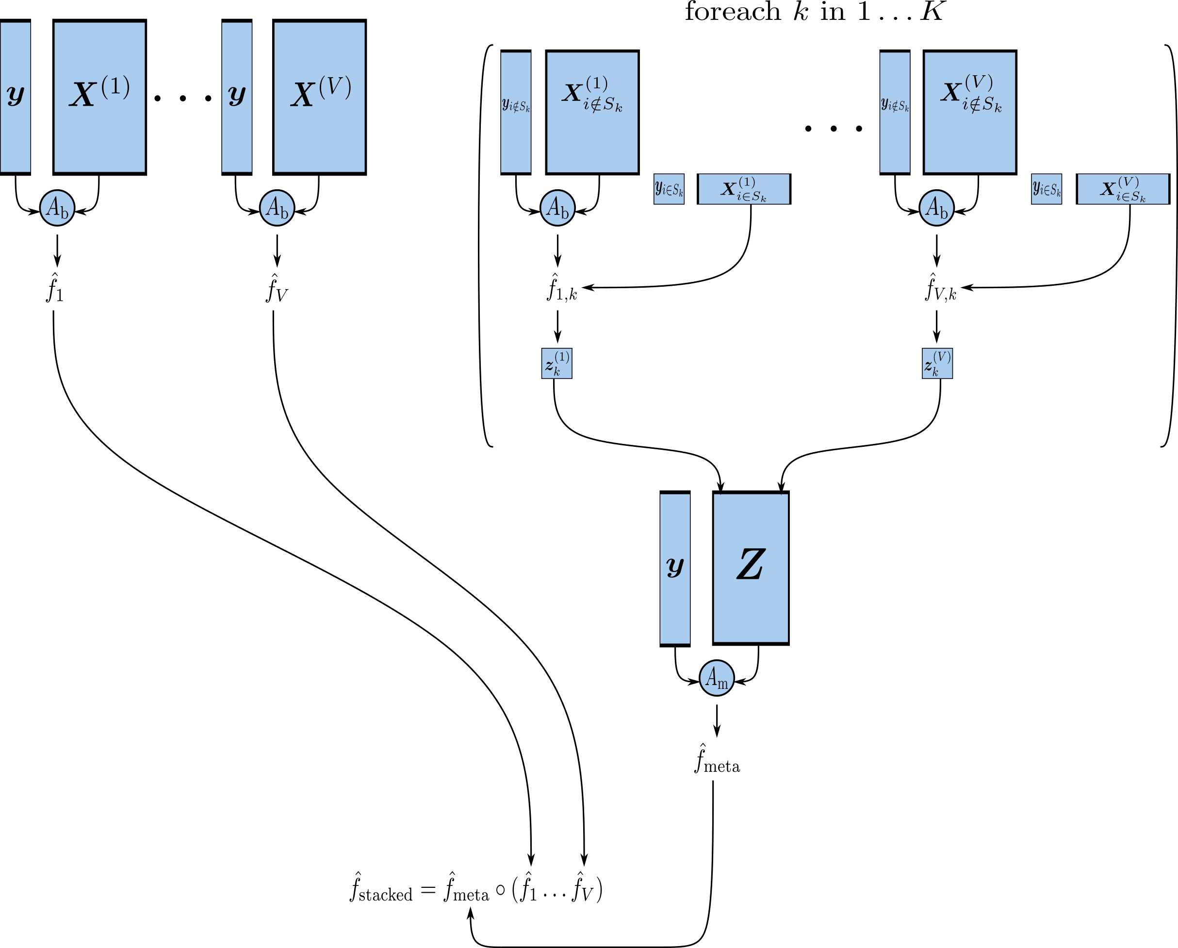
Figure 1: The 2-level StaPLR algorithm, with a single base learner, represented as a flow diagram.

2.3 Handling Missing Views Through Meta-Level Imputation with StaPLR

As shown in Algorithm 1 and Figure 1, StaPLR performs view selection through two steps: a dimension reduction step, and a feature selection step. First, a matrix of cross-validated predictions $\bm{Z}$ is constructed, in which each view is represented by a single column. The meta-learning algorithm then performs feature selection in this reduced space, which translates to view selection in the original feature space. Note that the reduction of dimensionality is generally very large: If the complete concatenated feature matrix $\bm{X}=(\bm{X}^{(1)},\dots,\bm{X}^{(V)})$ has dimensionality $n\times m$, then $\bm{Z}$ has dimensionality $n\times V$, and generally $V\ll m$. This further implies that, while the original data is usually very high dimensional, this is often not the case in the reduced space; see for example van Loon et al. [15] for an application of StaPLR where $n\ll m$, but $n>V$. Obviously, it is much less computationally intensive to fit models in the reduced space, than it is to fit them in the original space. It is therefore highly computationally attractive to perform any missing value imputation in this reduced space. Furthermore, as long as we assume $n>V$, imputation methods which would perform poorly in the high-dimensional feature space can instead be applied in the reduced space.

To apply the dimension reduction, the base-learning algorithm is trained on each view separately. Given that a view is either completely missing or completely observed, this means that within each application of the base learner there are no observations with partially observed data. Thus, the base learner can simply be trained on the set of complete cases for each view. A comparison of the proposed method for handling missing views in StaPLR and feature concatenation is shown in Figure 2.

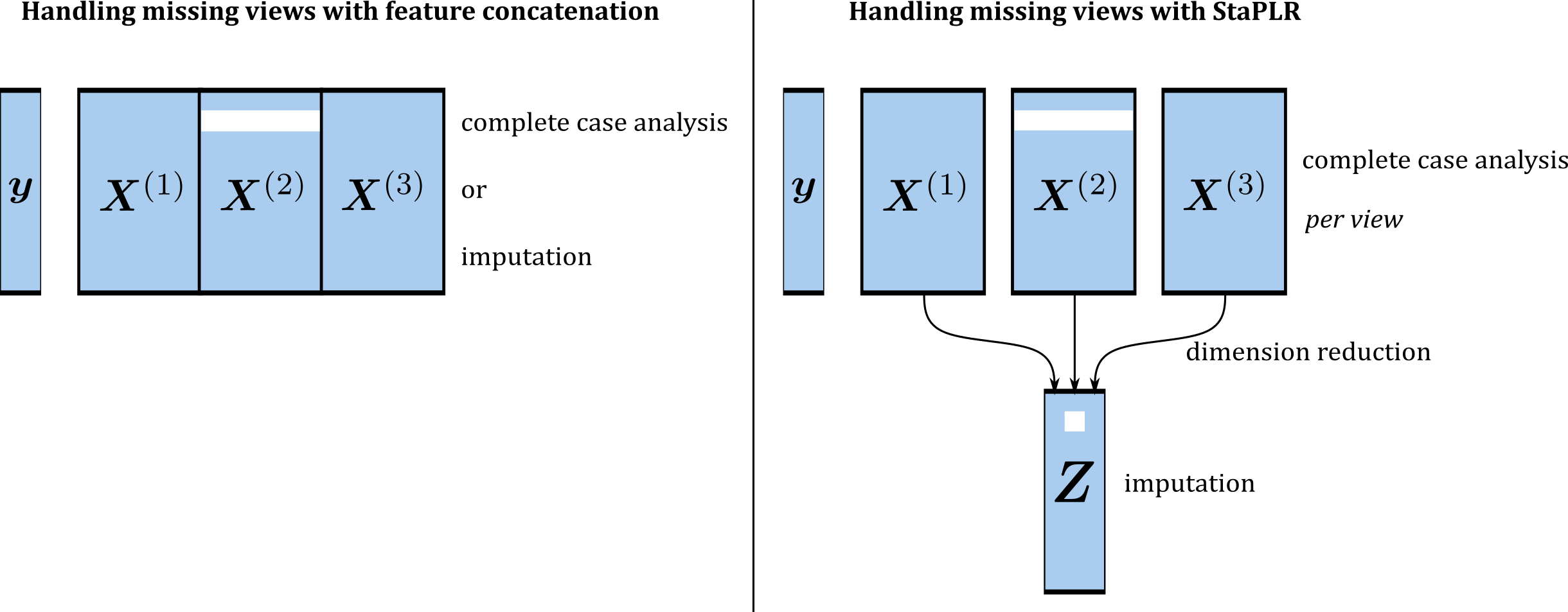
Figure 2: An example of how missing views can be handled through either classical feature concatenation (left), or through StaPLR (right). The blank areas in the data represent missing values. In this example, we assume there are three views, namely $\bm{X}^{(1)}$, $\bm{X}^{(2)}$, and $\bm{X}^{(3)}$. We denote the number of features in each view by $m_{1}$, $m_{2}$, and $m_{3}$, respectively. Assume that there are $l$ observations which have missing values on $\bm{X}^{(2)}$. In the case of feature concatenation, we would have to either impute $lm_{2}$ missing values, or entirely discard $l(m_{1}+m_{3})$ observed values. However, in the proposed missing data handling method for StaPLR, only $l$ values need to be imputed.

3 Empirical Evaluation

We evaluate the proposed meta-level imputation method by applying three popular imputation algorithms at the meta-level, and comparing the results with the application of those same algorithms at the feature level: The first imputation algorithm is simple unconditional mean imputation (MI), where each missing value is replaced by the mean of the observed values of the feature.

The second algorithm is predictive mean matching (PMM) [17], a state-of-the-art multiple imputation algorithm implemented as the default in the R package mice [24]. PMM is based on Bayesian imputation under the normal linear model [25, 26, 17], but instead of using a Bayesian draw of the regression coefficient to directly calculate an imputed value, it is used to find a set of $d$ candidate ‘donors’, which are the $d$ observations for which the predicted value under the imputation model is closest to the value drawn for the missing observation [17, 24]. The imputed value is then a random draw from the observed values of the donors. Advantages of PMM over direct Bayesian imputation include that the method allows for discrete target variables, the imputed values can never go outside the range of the observed data, and the method is more robust to model misspecification [17]. Disadvantages compared to other imputation methods include the fact that PMM tends to work poorly in high-dimensional settings, and that the required computation time is so large that we can only apply PMM at the meta-level, as feature-level imputation using PMM proved entirely infeasible (see Appendix A). When applying PMM, we use the default value of 5 for both the number of candidate donors and the number of imputations. With multiple imputation comes the need to somehow combine the results of the different imputed data sets. We evaluate two strategies for combining the different imputed data sets: The first strategy is to impute the matrix of cross-validated predictions $\bm{Z}$ 5 times, and then average the results before training the meta-learner. The second strategy is to generate the matrix $\bm{Z}$ 5 times, each time using different cross-validation folds, and then impute each matrix once before averaging the results. The benefit of the second strategy is that it also averages over different ways in which observations are allocated to cross-validation folds, but it is approximately 5 times more computationally expensive. To distinguish between the two strategies, we will refer to them as mPMM and cvPMM, respectively.

The third algorithm we consider is missForest (MF), an iterative imputation method based on random forests [19], as implemented in the R package missForest. MF can be used to impute both continuous and categorical data, and by averaging over many unpruned regression or classification trees it is intrinsically a multiple imputation method, while producing only a single completed data set [19]. When applying the MF algorithm, we use the default settings for the R package missForest, which constitutes growing 100 trees in each forest.

Finally, we also compare the results of the different imputation algorithms with complete case analysis (CCA), and with an application of StaPLR to the complete data before any missingness is generated, a process we will call complete data analysis (CDA). Note that for all the conditional imputation methods the outcome $y$ is also included in the imputation procedure, as is generally recommended in the missing value literature [27].

3.1 Simulation Design

We generate multi-view data consisting of $V=4$ disjoint views. Each view $v=1\dots V$ consists of $m_{v}=5\times 10^{v-1}$ random normally distributed features. The mean correlation between features within the same view is set to $\rho_{w}$ = 0.5. The mean correlation between features in different views is set to $\rho_{b}$ = 0.2. If view $v$ corresponds to signal, then each feature within that view has a regression coefficient of $2/\sqrt{m_{v}}$ or $-2/\sqrt{m_{v}}$, each with probability 0.5. If a view corresponds to noise, then each feature within that view has a regression coefficient of zero. The features and their respective coefficients together form a linear predictor (with an intercept equal to zero) to which the logistic function is applied to obtain probabilities. These probabilities are then used to draw the observations of the binary outcome $y$. This method for generating simulated data is similar to that used in earlier work on StaPLR [13, 14]. The following experimental factors are varied:

• Fraction of observations with a missing view: A single view is MCAR for either 50% or 90% of the observations.

• Size of the missing view: The missing view is either the smallest ($V_{1}$) or the largest ($V_{4}$) view.

• Size of the noise view: Either the smallest ($V_{1}$) or the largest ($V_{4}$) view corresponds to noise, while all other views correspond to signal.

This leads to a total of $2\times 2\times 2=8$ experimental conditions. For each experimental condition, 100 replications are performed. For each replication of each condition, we generate a training set of $n=1000$ observations in which the missingness occurs. All imputation and model fitting occurs in the training set. For each training set we generate a matching test set, also consisting of 1000 observations. There are no missing values in the test set, and the test set is only used for the calculation of certain outcome measures (Section 3.3).

3.2 Software

All simulations are performed in R (version 4.1.2) [28] on a high-performance computing cluster running Cent OS (Stream 8) with Slurm Workload Manager (version 20.11). All pseudo-random number generation is performed using the Mersenne Twister [29], R’s default algorithm. Imputation with the missForest algorithm is performed using the R package missForest (version 1.5) [19], while predictive mean matching is performed using mice (version 3.14) [24]. All StaPLR model fitting is performed using multiview (version 0.3.1) [30], with a glmnet (version 4.1-4) [31] back-end. Additional scripts, such as those used for mean imputation and data simulation, are included in the supplementary materials.

3.3 Outcome Measures

We compare the predictive performance of the trained stacked classifiers in terms of two outcome measures calculated on the test set. The first outcome measure is test accuracy, which we define as the proportion of correctly classified observations in the test set given a classification threshold of 0.5. The second outcome measure is the mean squared error of probabilities (MSEP), which we define as:

$$\text{MSEP}=\frac{1}{n}\sum_{i=1}^{n}(\hat{p}_{i}-p_{i})^{2},$$

where $p_{i}$ is the true class probability of test set observation $i$, and $\hat{p}_{i}$ is the value predicted by the classifier. Note that outside of simulation studies the true class probabilities would be unknown, and the MSEP cannot be calculated. However, replacing the true probabilities in the MSEP with the true class labels naturally leads to a well-known classification measure known as the Brier score [32]. Here we use the MSEP instead of the Brier score, as it is expected to be more sensitive to small changes in the data.

To assess view selection performance, we calculate four outcome measures. The first is simply the mean proportion of correctly selected views. The second outcome measure is the true positive rate (TPR), which is defined as the average proportion of views truly related to the outcome that were correctly selected by the meta-learner. The third outcome measure is the false positive rate (FPR), which is defined as the average proportion of views not related to the outcome that were incorrectly selected by the meta-learner. The fourth outcome measure is the false discovery rate, which is defined as the average proportion of incorrectly selected views among the set of selected views if at least one view is selected, and zero otherwise. In addition to classification and view selection performance, we also calculate the logarithm of the computation time in seconds for each procedure.

4 Results

Figures 3 and 4 show, respectively, the classification accuracy and MSEP of the different methods for handling missing data under 90% missingness. Figures 5 and 6 show the same outcome measures under 50% missingness. We will focus on the results under 90% missingness as they generally show the same patterns of how the different imputation methods behave, but in an emphasized manner. In terms of test accuracy, complete case analysis performs worse than all imputation methods, while the differences between the imputation methods are comparatively small, although when the noise view consists of many features, and the smallest view ($V_{1}$) is missing, mean imputation appears to perform slightly better than the other imputation methods.

As expected, the MSEP is more sensitive to changes in the imputed data than the test accuracy. Again CCA performs the worst, while CDA performs the best. Mean imputation performs as good as or better than the other imputation methods. Base-level missForest (MF) performs as good as, or better than meta-level missForest (mMF) or predictive mean matching (mPMM and cvPMM). When the noise view consists of a high number of features, mMF, mPMM and cvPMM have larger variance of the MSEP than the other prediction methods.

For the sake of completeness, we also calculated the binomial deviance. It supports the same general conclusions, lying in between the accuracy and MSEP in terms of sensitivity to the imputed data (see Appendix B).

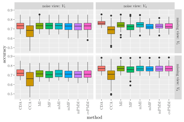
Figure 3: Test accuracy with 90% missingness. CDA = complete data analysis; CCA = complete case analysis; MI = feature-level mean imputation; MF = feature-level missForest; mMI = meta-level mean imputation; mMF = meta-level missForest; mPMM = meta-level predictive mean matching, generating $\bm{Z}$ once; cvPMM = meta-level predictive mean matching, generating $\bm{Z}$ five times. $V_{1}$ is the smallest view, consisting of 5 features. $V_{4}$ is the largest view, consisting of 5000 features.

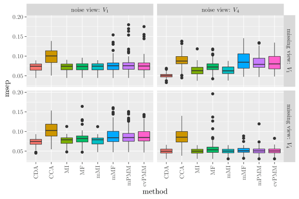
Figure 4: Mean squared error of probabilities (MSEP) with 90% missingness. CDA = complete data analysis; CCA = complete case analysis; MI = feature-level mean imputation; MF = feature-level missForest; mMI = meta-level mean imputation; mMF = meta-level missForest; mPMM = meta-level predictive mean matching, generating $\bm{Z}$ once; cvPMM = meta-level predictive mean matching, generating $\bm{Z}$ five times. $V_{1}$ is the smallest view, consisting of 5 features. $V_{4}$ is the largest view, consisting of 5000 features.

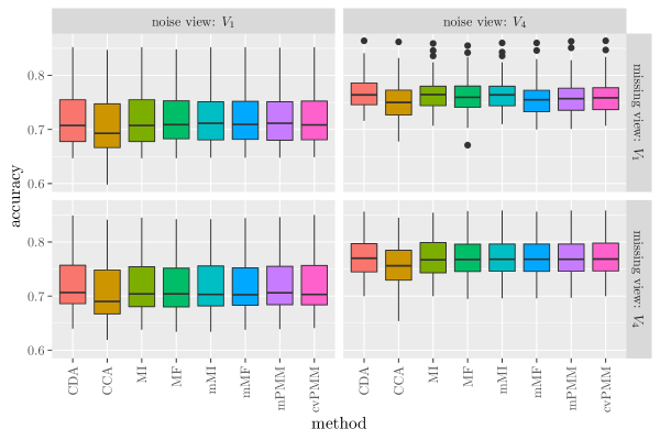
Figure 5: Test accuracy with 50% missingness. CDA = complete data analysis; CCA = complete case analysis; MI = feature-level mean imputation; MF = feature-level missForest; mMI = meta-level mean imputation; mMF = meta-level missForest; mPMM = meta-level predictive mean matching, generating $\bm{Z}$ once; cvPMM = meta-level predictive mean matching, generating $\bm{Z}$ five times. $V_{1}$ is the smallest view, consisting of 5 features. $V_{4}$ is the largest view, consisting of 5000 features.

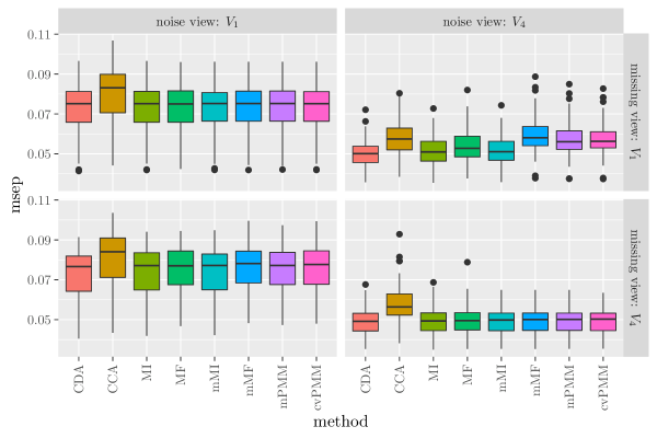
Figure 6: Mean squared error of probabilities (MSEP) with 50% missingness. CDA = complete data analysis; CCA = complete case analysis; MI = feature-level mean imputation; MF = feature-level missForest; mMI = meta-level mean imputation; mMF = meta-level missForest; mPMM = meta-level predictive mean matching, generating $\bm{Z}$ once; cvPMM = meta-level predictive mean matching, generating $\bm{Z}$ five times. $V_{1}$ is the smallest view, consisting of 5 features. $V_{4}$ is the largest view, consisting of 5000 features.

4.1 View Selection

In terms of the mean proportion of correctly selected views (Table 1), CCA again performs worse than all imputation methods. Among the imputation methods, a trend can be observed where mean imputation (both MI and mMI) performs well when the view to be imputed corresponds to noise, but performs poorly when the view to be imputed corresponds to signal. The mMF, mPMM and cvPMM methods all appear to perform similarly. mMF sometimes shows somewhat better performance than MF, particularly when the missing view has a large number of features, but the pattern of differences between the two methods is not entirely consistent.

In terms of the TPR (Table 2), CCA again performs worse than all imputation methods. Both MI and mMI perform well in terms of TPR when compared with the other imputation methods. The mMF, mPMM and cvPMM method again show similar performance. The observed differences between MF and mMF do not appear to follow a consistent pattern.

In terms of the FPR (Table 3), a pattern can be observed where mean imputation (MI and mMI) performs really well when the view to be imputed corresponds to noise, but performs poorly when the view to be imputed corresponds to signal. The performance of MF shows the opposite behavior: it performs better when the view to be imputed corresponds to signal than when it corresponds to noise. Similar behavior can be observed for its meta-level implementation mMF. Comparing MF and mMF shows that MF has a slightly lower FPR when the size of the missing view is 5, but has a considerably higher FPR than mMF when the size of the missing view is 5000. The observed differences in FPR between mMF and mPMM and cvPMM are small under 50% missingness. Under 90% missingness larger differences are observed when the signal view with 5 features is missing, and when the noise view with 5000 features is missing. In terms of FPR, CCA performs well when compared to the imputation methods.

The relative performance of the imputation methods in terms of FDR (Table 4) is similar to that in terms of FPR. CCA also performs fairly well in terms of FDR, just like it does in terms of FPR.

missingness	size of missing view	missing view is	CDA	CCA	MI	MF	mMI	mMF	mPMM	cvPMM
50%	5	noise	.903	.850	.900	.903	.908	.898	.898	.905
		signal	.960	.918	.943	.960	.925	.953	.953	.955
	5000	noise	.958	.908	.955	.910	.958	.950	.948	.943
		signal	.893	.845	.848	.868	.848	.875	.875	.875
90%	5	noise	.885	.625	.895	.865	.880	.858	.855	.873
		signal	.970	.703	.868	.873	.875	.895	.908	.918
	5000	noise	.965	.683	.983	.870	.978	.930	.953	.963
		signal	.908	.608	.785	.830	.788	.843	.830	.845

Table 1: Mean proportion of correctly selected views. CDA = complete data analysis; CCA = complete case analysis; MI = feature-level mean imputation; MF = feature-level missForest; mMI = meta-level mean imputation; mMF = meta-level missForest; mPMM = meta-level predictive mean matching, generating $\bm{Z}$ once; cvPMM = meta-level predictive mean matching, generating $\bm{Z}$ five times.

missingness	size of missing view	missing view is	CDA	CCA	MI	MF	mMI	mMF	mPMM	cvPMM
50%	5	noise	.877	.827	.880	.890	.887	.887	.887	.890
		signal	.963	.927	.970	.950	.963	.943	.943	.943
	5000	noise	.957	.900	.960	.960	.960	.960	.960	.953
		signal	.877	.810	.853	.880	.863	.850	.853	.850
90%	5	noise	.877	.533	.877	.873	.870	.867	.863	.873
		signal	.967	.627	.933	.833	.940	.877	.903	.923
	5000	noise	.967	.613	.977	.970	.973	.973	.973	.980
		signal	.900	.493	.807	.847	.810	.810	.797	.807

Table 2: True positive rate (TPR). CDA = complete data analysis; CCA = complete case analysis; MI = feature-level mean imputation; MF = feature-level missForest; mMI = meta-level mean imputation; mMF = meta-level missForest; mPMM = meta-level predictive mean matching, generating $\bm{Z}$ once; cvPMM = meta-level predictive mean matching, generating $\bm{Z}$ five times.

missingness	size of missing view	missing view is	CDA	CCA	MI	MF	mMI	mMF	mPMM	cvPMM
50%	5	noise	.02	.08	.04	.06	.03	.07	.07	.05
		signal	.05	.11	.14	.01	.19	.02	.02	.01
	5000	noise	.04	.07	.06	.24	.05	.08	.09	.09
		signal	.06	.05	.17	.17	.20	.05	.06	.05
90%	5	noise	.09	.10	.05	.16	.09	.17	.17	.13
		signal	.02	.07	.33	.01	.32	.05	.08	.10
	5000	noise	.04	.11	0	.43	.01	.20	.11	.09
		signal	.07	.05	.28	.22	.28	.06	.07	.04

Table 3: False positive rate (FPR). CDA = complete data analysis; CCA = complete case analysis; MI = feature-level mean imputation; MF = feature-level missForest; mMI = meta-level mean imputation; mMF = meta-level missForest; mPMM = meta-level predictive mean matching, generating $\bm{Z}$ once; cvPMM = meta-level predictive mean matching, generating $\bm{Z}$ five times.

missingness	size of missing view	missing view is	CDA	CCA	MI	MF	mMI	mMF	mPMM	cvPMM
50%	5	noise	.005	.022	.010	.015	.008	.018	.018	.013
		signal	.013	.029	.035	.003	.047	.005	.006	.003
	5000	noise	.011	.018	.015	.063	.013	.020	.023	.023
		signal	.016	.013	.044	.045	.053	.013	.016	.013
90%	5	noise	.023	.034	.013	.041	.024	.048	.047	.035
		signal	.005	.022	.084	.003	.08	.013	.021	.026
	5000	noise	.012	.031	0	.112	.003	.051	.028	.023
		signal	.018	.032	.073	.060	.073	.016	.020	.011

Table 4: False discovery rate (FDR). CDA = complete data analysis; CCA = complete case analysis; MI = feature-level mean imputation; MF = feature-level missForest; mMI = meta-level mean imputation; mMF = meta-level missForest; mPMM = meta-level predictive mean matching, generating $\bm{Z}$ once; cvPMM = meta-level predictive mean matching, generating $\bm{Z}$ five times.

4.2 Computation Time

Figure 7 shows the log computation time for all imputation methods, as well as CDA and CCA, with 90% missingness. Figure 8 shows the log computation time with 50% missingness. Note that the computation times reported here include the computations of both the model fitting and the imputation model. It can be observed that CCA has the lowest computation time across all plots, since it constitutes a reduction in the amount of observations in the training data. By comparing MI with mMI, and MF with mMF, it can be observed that meta-level imputation is faster than base-level imputation. This is particularly noticeable when the view to be imputed is large (i.e. when $V_{4}$ is missing), when MF is the slowest method by a large margin. cvPMM is considerably slower than mPMM, and is the slowest method when the view to be imputed is small (i.e. when $V_{1}$ is missing).

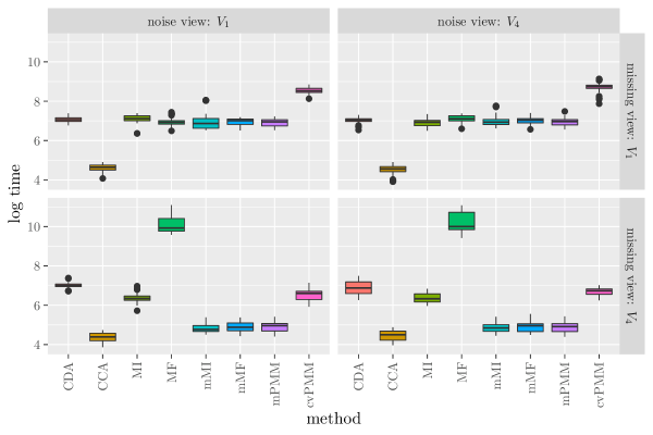
Figure 7: Logarithm of computation time (in seconds) with 90% missingness. CDA = complete data analysis; CCA = complete case analysis; MI = feature-level mean imputation; MF = feature-level missForest; mMI = meta-level mean imputation; mMF = meta-level missForest; mPMM = meta-level predictive mean matching, generating $\bm{Z}$ once; cvPMM = meta-level predictive mean matching, generating $\bm{Z}$ five times. $V_{1}$ is the smallest view, consisting of 5 features. $V_{4}$ is the largest view, consisting of 5000 features.

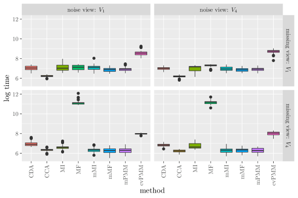
Figure 8: Logarithm of computation time (in seconds) with 50% missingness. CDA = complete data analysis; CCA = complete case analysis; MI = feature-level mean imputation; MF = feature-level missForest; mMI = meta-level mean imputation; mMF = meta-level missForest; mPMM = meta-level predictive mean matching, generating $\bm{Z}$ once; cvPMM = meta-level predictive mean matching, generating $\bm{Z}$ five times. $V_{1}$ is the smallest view, consisting of 5 features. $V_{4}$ is the largest view, consisting of 5000 features.

5 Discussion

Our results support four general conclusions: First, complete data analysis performs best. This is unsurprising, since, as Orchard and Woodbury [33, p. 697] noted, “the best way to treat missing data is not to have them.” Second, perhaps also unsurprising but more interesting, is that any form of imputation works better than complete case analysis. Third, which is likely more surprising and interesting, is that if the goal is solely to predict the outcome, the best form of imputation is unconditional mean imputation (MI or mMI): it is fast (particularly mMI) and performed well in terms of both test accuracy and MSEP across all experimental conditions. The idea that mean imputation can be useful for prediction is not new; Josse et al. [18] have shown that mean imputation is universally consistent for prediction as long as the employed learning algorithm is universally consistent. However, those conditions do not apply here, so it is interesting to see that mean imputation can also work well for prediction in a multi-view setting with a small sample size. If the aim is not just prediction but also view selection, then the performance of mean imputation depends on whether the view to be imputed corresponds to signal or to noise. If the view to be imputed corresponds to noise, MI performs well in all measures of view selection performance, but if the view to be imputed corresponds to signal, MI leads to the highest FPR and FDR of all imputation methods considered in this article. This difference in performance can be explained by considering MI as a form of regularization applied only to the view(s) in which missing values occur, since MI reduces the variance of any imputed features and attenuates the correlation with the outcome. Thus, if the view corresponds to noise, this regularization is beneficial as it reduces the probability that the view is picked up by the meta-learner. However, if the view corresponds to signal, then MI attenuates the signal, causing the meta-learner to include superfluous views. Obviously, a method which automatically selects views is primarily useful in a setting where the status of a view as signal or noise is unknown beforehand. Thus, although unconditional mean imputation works well for prediction, it should not be used if the aim of a study includes view selection. The finding that conditional imputation works better than unconditional imputation for view selection is consistent with earlier results on the effect of imputation on feature selection [23].

The fourth and final major conclusion is that meta-level imputation is much faster than feature-level imputation, but can still obtain good results. In fact, meta-level imputation allows the use of sophisticated imputation algorithms such as PMM which are infeasible to use at the feature level. In this article we have used a relatively simple simulation scheme with only a single missing view. However, since in practice the number of views is generally much smaller than the number of features, we expect that the advantages of meta-level imputation will generally increase in larger multi-view data sets with more than one missing view.

Our simulations show that feature-level MF sometimes performs better than mMF or mPMM/cvPMM in terms of MSEP, but these observed differences in terms of predicted probabilities did not affect classification performance. For view selection, the observed differences between MF and mMF/mPMM/cvPMM are not entirely consistent. However, it is worth noting that in some cases base level MF lead to considerably higher values of FPR and TPR than mMF. Consider the FPR: in those cases where a higher value of FPR is observed for mMF the differences are very small ($\leq 0.04$), but in those cases where a higher value of FPR is observed for MF, the differences are much larger ($\leq 0.23$). A similar pattern can be observed for the FDR. For additional context, it may be worth pointing out that in experiments which aim to control the FDR, a typical value at which to control the FDR is 0.05. Using this as a reference value, only mPMM and cvPMM show observed FDR values which are consistently below 0.05.

For the meta-level implementation of predictive mean matching, we used two different ways of combining the imputed data sets. The first one is generating the $\bm{Z}$ matrix once, imputing it 5 times, then averaging the imputed data sets and training the meta-learner on the averaged data set (mPMM). The second is generating the $\bm{Z}$ matrix 5 times, imputing each of these matrices once, and then averaging the imputed data sets and training the meta-learner on the averaged data set (cvPMM). The cvPMM approach is much more computationally expensive (Figures 8 and 7), but also averages over different allocations to the cross-validation folds, instead of just over different imputations. However, this approach did not lead to an improvement in classification performance, and only small differences in view selection performance, which makes mPMM preferable for use in practice. Of course, other methods of combining imputations are possible. For example, one could train the meta learner separately on each imputated data set, leading to 5 separate StaPLR models. However, this leads to additional questions in how to combine the separate models, and given the observed differences between mPMM and cvPMM, we would not expect this approach to cause large gains in performance.

Throughout this article we have assumed that while the number of features $m$ was larger than $n$, the number of views $V$ was always smaller. It is natural then to wonder how the meta-level imputation methods would perform if $n<V$ (i.e. if $\bm{Z}$ were high-dimensional). Given that missForest can handle high-dimensional data, as is evident by the performance of MF in this article, mMF could most likely be used without issue. The same cannot be said for mPMM or cvPMM, since standard PMM based on the linear model struggles even with small high-dimensional data sets (A). However, alternative approaches could be constructed. For example, an imputation method based on the lasso [34, 35] is included in mice [24], and appeared to work quite well for a small high-dimensional data set such as the one described in A (results not shown), although the associated computation time still made it infeasible to include as a base-level imputation method in this study. Nevertheless, since generally $V\ll m$, it has potential as a meta-level imputation method in cases where $\bm{Z}$ is high-dimensional.

In our simulations missingness occurred only in the training set, but in practical settings it is likely that missingness occurs also in the test set. In this case, Josse et al. [18] recommend that the same imputation model that was used to impute the training set is used to impute the test set. Unfortunately, this is not so easy to do in practice, since many implementations of imputation methods, including mice [24] and missForest [19], effectively work as ‘black boxes’ that do not separate the imputation model from its use to complete the data [18]. A possible solution that has been suggested for this problem is to take a semi-supervised approach [18], jointly imputing the train and test set [36], and then learning the prediction model on the training set only, but this does require that the training set is available at test time [18].

Throughout most of this article we assumed that the data was MCAR, and gave examples of why this is often a realistic assumption in the case of multi-view missing data. Nevertheless, in practice there will also be cases where the data is MAR or even MNAR. Multiple imputation methods such as MF and PMM are known to provide unbiased parameter estimates even under MAR. Of course, this is assuming the learning algorithm generates unbiased estimates in general, which is not the case for StaPLR, where the exact values of the parameter estimates are generally not of interest. How the theoretical knowledge about multiple imputation methods at the feature-level translates to imputation at the meta-level under MAR or MNAR, and how it affects view selection and classification accuracy in these settings is a topic for future research.

In summary, we have proposed a meta-level imputation method for missing values in multi-view data. We have evaluated the method with several imputation algorithms using simulations. The results show that meta-level imputation produces competitive results in terms of test accuracy and view selection at a much lower computational cost, and makes the use of advanced multiple imputation methods such as predictive mean matching possible in high-dimensional settings where they were previously computationally infeasible.

6 Declaration of Interest

This research was funded by Leiden University. The authors declare no conflicts of interest.

Appendix A Infeasibility of Predictive Mean Matching Using MICE

We first show empirically how predictive mean matching using mice leads to imputations of poor quality when the data is high-dimensional. We generate a high-dimensional, but comparatively small single-view data set with $n=200$ independent observations of $m=400$ normally distributed features and one binary outcome $y$. Only the first 50 values of the first feature are missing. Compared to the main simulations presented in this paper, this is a very easy missing data problem.

We generate an imputed data set with PMM using mice. Figure 9 shows that the imputed values (first 50 observations; triangles) of feature one are generally at the extreme end of the distribution of observed values, and their distribution is non-normal and very different from that of the observed values (last 150 observations; circles). R code to replicate this image is included in the supplementary materials. The likely cause of this behavior is that the linear model is not well-behaved under high-dimensionality, meaning some form of (ridge) regularization is required [17, 24], but the amount of regularization required to find a ‘good’ solution is not obvious. Recommended values for the penalty parameter in the range $10^{-6}$ to $10^{-4}$ do not produce good results, even in this relatively simple setting.

Even when good results could be obtained, two practical problems make calculations using mice infeasible for large high-dimensional problems. The first, and most important one, is time: Even for the simplest setting included in our experiments, a single iteration of a single imputation of a single variable took well over 24 hours to compute. The second, which was not directly relevant to our study but will be for larger problems, is memory handling: A test run of PMM with mice on a data set consisting of 200 observations of 75,000 variables (120 MB of data), which is small by medical imaging standards, already required 42 GB of RAM.

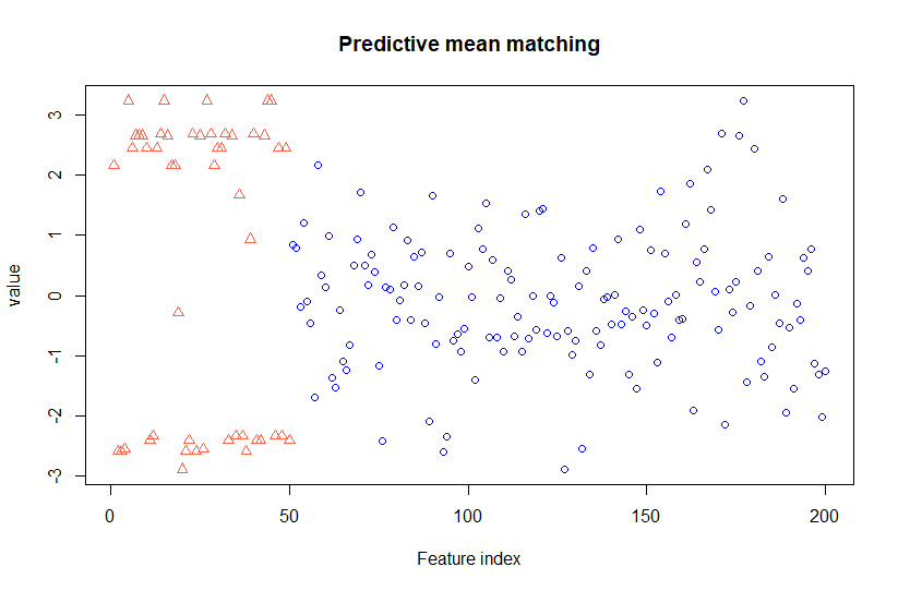
Figure 9: Imputed (red triangles) and observed (blue circles) values of feature 1 after imputing the missing values with PMM using mice.

Appendix B Binomial Deviance

The binomial deviance is defined as:

$$D=-2\sum_{i=1}^{n}y_{i}\log(\hat{p}_{i})+(1-y_{i})\log(1-\hat{p}_{i}),$$

where $y_{i}$ is the observed class label for test set observation $i$, and $\hat{p}_{i}$ is the predicted probability of belonging to class 1.

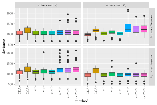
Figure 10: Binomial deviance with 90% missingness. CDA = complete data analysis; CCA = complete case analysis; MI = feature-level mean imputation; MF = feature-level missForest; mMI = meta-level mean imputation; mMF = meta-level missForest; mPMM = meta-level predictive mean matching, generating $\bm{Z}$ once; cvPMM = meta-level predictive mean matching, generating $\bm{Z}$ five times. $V_{1}$ is the smallest view, consisting of 5 features. $V_{4}$ is the largest view, consisting of 5000 features.

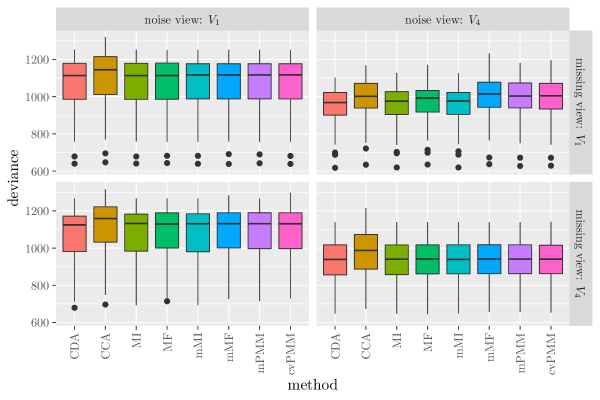
Figure 11: Binomial deviance with 50% missingness. CDA = complete data analysis; CCA = complete case analysis; MI = feature-level mean imputation; MF = feature-level missForest; mMI = meta-level mean imputation; mMF = meta-level missForest; mPMM = meta-level predictive mean matching, generating $\bm{Z}$ once; cvPMM = meta-level predictive mean matching, generating $\bm{Z}$ five times. $V_{1}$ is the smallest view, consisting of 5 features. $V_{4}$ is the largest view, consisting of 5000 features.

References

- Zhao et al. [2017] J. Zhao, X. Xie, X. Xu, and S. Sun, “Multi-view learning overview: recent progress and new challenges,” Information Fusion, vol. 38, pp. 43–54, 2017.
- Sun et al. [2019] S. Sun, L. Mao, Z. Dong, and L. Wu, Multiview Machine Learning. Springer, 2019.
- Li et al. [2018] Y. Li, F.-X. Wu, and A. Ngom, “A review on machine learning principles for multi-view biological data integration,” Briefings in Bioinformatics, vol. 19, no. 2, pp. 325–340, 2018.
- Sudlow et al. [2015] C. Sudlow, J. Gallacher, N. Allen, V. Beral, P. Burton, J. Danesh, P. Downey, P. Elliott, J. Green, M. Landray et al., “UK biobank: an open access resource for identifying the causes of a wide range of complex diseases of middle and old age,” PLoS Medicine, vol. 12, no. 3, p. e1001779, 2015.
- Littlejohns et al. [2020] T. J. Littlejohns, J. Holliday, L. M. Gibson, S. Garratt, N. Oesingmann, F. Alfaro-Almagro, J. D. Bell, C. Boultwood, R. Collins, M. C. Conroy et al., “The UK biobank imaging enhancement of 100,000 participants: rationale, data collection, management and future directions,” Nature Communications, vol. 11, no. 1, pp. 1–12, 2020.
- Mueller et al. [2005] S. G. Mueller, M. W. Weiner, L. J. Thal, R. C. Petersen, C. Jack, W. Jagust, J. Q. Trojanowski, A. W. Toga, and L. Beckett, “The Alzheimer’s disease neuroimaging initiative,” Neuroimaging Clinics of North America, vol. 15, no. 4, p. 869, 2005.
- Schouten et al. [2016] T. M. Schouten, M. Koini, F. De Vos, S. Seiler, J. van der Grond, A. Lechner, A. Hafkemeijer, C. Möller, R. Schmidt, M. de Rooij, and S. A. Rombouts, “Combining anatomical, diffusion, and resting state functional magnetic resonance imaging for individual classification of mild and moderate Alzheimer’s disease,” NeuroImage: Clinical, vol. 11, pp. 46–51, 2016.
- de Vos et al. [2016] F. de Vos, T. M. Schouten, A. Hafkemeijer, E. G. Dopper, J. C. van Swieten, M. de Rooij, J. van der Grond, and S. A. Rombouts, “Combining multiple anatomical MRI measures improves Alzheimer’s disease classification,” Human Brain Mapping, vol. 37, pp. 1920–1929, 2016.
- de Vos et al. [2017] F. de Vos, M. Koini, T. M. Schouten, S. Seiler, J. van der Grond, A. Lechner, R. Schmidt, M. de Rooij, and S. A. Rombouts, “A comprehensive analysis of resting state fMRI measures to classify individual patients with Alzheimer’s disease,” NeuroImage, vol. 167, pp. 62–72, 2017.
- Salvador et al. [2019] R. Salvador, E. Canales-Rodríguez, A. Guerrero-Pedraza, S. Sarró, D. Tordesillas-Gutiérrez, T. Maristany, B. Crespo-Facorro, P. McKenna, and E. Pomarol-Clotet, “Multimodal integration of brain images for MRI-based diagnosis in schizophrenia,” Frontiers in Neuroscience, vol. 13, no. 1203, pp. 1–9, 2019.
- Guggenmos et al. [2020] M. Guggenmos, K. Schmack, I. M. Veer, T. Lett, M. Sekutowicz, M. Sebold, M. Garbusow, C. Sommer, H.-U. Wittchen, U. S. Zimmermann, M. N. Smolka, H. Walter, A. Heinz, and P. Sterzer, “A multimodal neuroimaging classifier for alcohol dependence,” Scientific Reports, vol. 10, no. 298, pp. 1–12, 2020.
- Ali et al. [2021] L. Ali, Z. He, W. Cao, H. T. Rauf, Y. Imrana, and M. B. B. Heyat, “MMDD-ensemble: A multimodal data driven ensemble approach for Parkinson’s disease detection,” Frontiers in Neuroscience, vol. 15, no. 754058, pp. 1–11, 2021.
- van Loon et al. [2020a] W. van Loon, M. Fokkema, B. Szabo, and M. de Rooij, “Stacked penalized logistic regression for selecting views in multi-view learning,” Information Fusion, vol. 61, pp. 113–123, 2020.
- van Loon et al. [2020b] ——, “View selection in multi-view stacking: choosing the meta-learner,” arXiv preprint arXiv:2010.16271, 2020.
- van Loon et al. [2022] W. van Loon, F. de Vos, M. Fokkema, B. Szabo, M. Koini, R. Schmidt, and M. de Rooij, “Analyzing hierarchical multi-view MRI data with StaPLR: An application to Alzheimer’s disease classification,” Frontiers in Neuroscience, vol. 16, no. 83063, 2022.
- Rubin [1976] D. B. Rubin, “Inference and missing data,” Biometrika, vol. 63, no. 3, pp. 581–592, 1976.
- Van Buuren [2018] S. Van Buuren, Flexible imputation of missing data. CRC press, 2018.
- Josse et al. [2019] J. Josse, N. Prost, E. Scornet, and G. Varoquaux, “On the consistency of supervised learning with missing values,” arXiv preprint arXiv:1902.06931, 2019.
- Stekhoven and Bühlmann [2012] D. J. Stekhoven and P. Bühlmann, “MissForest — non-parametric missing value imputation for mixed-type data,” Bioinformatics, vol. 28, no. 1, pp. 112–118, 2012.
- Arbuckle [1996] J. Arbuckle, “Full information estimation in the presence of incomplete data,” in Advanced structural equation modeling: Issues and techniques (2009 reprint), G. A. Marcoulides and R. E. Schumacker, Eds. New York, NY: Psychology Press, 1996, ch. 9, pp. 243–277.
- Myrtveit et al. [2001] I. Myrtveit, E. Stensrud, and U. H. Olsson, “Analyzing data sets with missing data: An empirical evaluation of imputation methods and likelihood-based methods,” IEEE Transactions on Software Engineering, vol. 27, no. 11, pp. 999–1013, 2001.
- Twala et al. [2008] B. E. Twala, M. Jones, and D. J. Hand, “Good methods for coping with missing data in decision trees,” Pattern Recognition Letters, vol. 29, no. 7, pp. 950–956, 2008.
- Mera-Gaona et al. [2021] M. Mera-Gaona, U. Neumann, R. Vargas-Canas, and D. M. López, “Evaluating the impact of multivariate imputation by MICE in feature selection,” PLOS ONE, vol. 16, no. 7, p. e0254720, 2021.
- van Buuren and Groothuis-Oudshoorn [2011] S. van Buuren and K. Groothuis-Oudshoorn, “mice: Multivariate imputation by chained equations in R,” Journal of Statistical Software, vol. 45, no. 3, pp. 1–67, 2011.
- Rubin [1987] D. B. Rubin, Multiple Imputation for Nonresponse in Surveys. John Wiley & Sons, Inc., 1987.
- Schafer [1997] J. L. Schafer, Analysis of incomplete multivariate data. Chapman & Hall / CRC press, 1997.
- Sterne et al. [2009] J. A. Sterne, I. R. White, J. B. Carlin, M. Spratt, P. Royston, M. G. Kenward, A. M. Wood, and J. R. Carpenter, “Multiple imputation for missing data in epidemiological and clinical research: potential and pitfalls,” Bmj, vol. 338, 2009.
- Team [2017] R. C. Team, R: A Language and Environment for Statistical Computing, R Foundation for Statistical Computing, Vienna, Austria, 2017. [Online]. Available: https://www.R-project.org/
- Matsumoto and Nishimura [1998] M. Matsumoto and T. Nishimura, “Mersenne twister: a 623-dimensionally equidistributed uniform pseudo-random number generator,” ACM Transactions on Modeling and Computer Simulation, vol. 8, no. 1, pp. 3–30, 1998.
- van Loon [2021] W. van Loon, R package ‘multiview’ - Methods for high-dimensional multi-view learning (v0.3.1), Feb. 2021. [Online]. Available: https://doi.org/10.5281/zenodo.4630669
- Friedman et al. [2010] J. Friedman, T. Hastie, and R. Tibshirani, “Regularization paths for generalized linear models via coordinate descent,” Journal of Statistical Software, vol. 33, no. 1, pp. 1–22, 2010. [Online]. Available: http://www.jstatsoft.org/v33/i01/
- Brier [1950] G. W. Brier, “Verification of forecasts expressed in terms of probability,” Monthly Weather Review, vol. 78, no. 1, pp. 1–3, 1950.
- Orchard and Woodbury [1972] T. Orchard and M. A. Woodbury, “A missing information principle: theory and applications,” in Volume 1 Theory of Statistics. University of California Press, 1972, pp. 697–716.
- Zhao and Long [2016] Y. Zhao and Q. Long, “Multiple imputation in the presence of high-dimensional data,” Statistical Methods in Medical Research, vol. 25, no. 5, pp. 2021–2035, 2016.
- Deng et al. [2016] Y. Deng, C. Chang, M. S. Ido, and Q. Long, “Multiple imputation for general missing data patterns in the presence of high-dimensional data,” Scientific Reports, vol. 6, no. 1, pp. 1–10, 2016.
- Kapelner and Bleich [2015] A. Kapelner and J. Bleich, “Prediction with missing data via bayesian additive regression trees,” Canadian Journal of Statistics, vol. 43, no. 2, pp. 224–239, 2015.