Sinusoidal Frequency Estimation by Gradient Descent

Abstract

Sinusoidal parameter estimation is a fundamental task in applications from spectral analysis to time-series forecasting. Estimating the sinusoidal frequency parameter by gradient descent is, however, often impossible as the error function is non-convex and densely populated with local minima. The growing family of differentiable signal processing methods has therefore been unable to tune the frequency of oscillatory components, preventing their use in a broad range of applications. This work presents a technique for joint sinusoidal frequency and amplitude estimation using the Wirtinger derivatives of a complex exponential surrogate and any first order gradient-based optimizer, enabling end-to-end training of neural network controllers for unconstrained sinusoidal models.

Index Terms—  differentiable signal processing, machine learning, sinusoidal parameter estimation

1 Introduction

Estimating sinusoidal parameters from a signal is a crucial step in numerous signal processing algorithms, and a wealth of techniques have been proposed in both the single and multiple sinusoid formulations. Most seek the maximum likelihood (ML) estimate of sinusoidal model parameters in the presence of white Gaussian noise, the statistical properties of which are well established [1].

Estimators of sinusoidal frequency must circumvent the non-linearity of the model and non-convexity of the corresponding objective as a function of the frequency parameter. The most common approach is thus to apply a multi-stage algorithm in which an initial frequency estimate is obtained through search heuristics [2, 3, 4], spectral peak interpolation [5], discrete-time Fourier transform (DTFT) decorrelation [6], or other procedures [7, 8, 9], and then refined using an optimization method. Alternate approaches include iteratively updating a model-based relaxation of the problem [10, 8], linearizing the problem using delay operators [11, 12], or defining a surrogate model where an equivalence can be drawn between solutions [13].

Such methods achieve accurate estimates but are unsuitable for use in the context of end-to-end models fit by gradient descent, where integrating derivative-free operations or complex heuristics is challenging and often unstable. In particular, the recent proliferation of models applying differentiable digital signal processing (DDSP) [14] – a family of techniques which allow neural networks to directly control digital signal processors – highlights the need for a method for sinusoidal frequency estimation by gradient descent.

Applications of DDSP have included providing high level controls for harmonic-plus-noise synthesizers [14], controlling digital synthesis methods with neural networks [15, 16], modelling [17] and controlling [18] audio effects and direct filter design [19]. Yet, despite success at these complex tasks, DDSP-based models have so far been unable to predict sinusoidal frequency parameters. Aspects of the problem have been acknowledged in the literature. Turian & Henry [20] showed that frequency domain distances lack a stable and informative frequency gradient, whilst Engel et al. [21] used a parameter regression pretraining scheme to circumvent issues with local minima when optimizing sinusoidal frequencies. Caspe et al. [16] similarly note that gradient descent fails to tune the modulation frequencies of a differentiable FM synthesizer due to ripple in the error function.

In this work, we propose a simple surrogate to the sinusoidal oscillator with gradients that allow first-order gradient based optimization. With this approach, we take a first step towards end-to-end learning of neural network controllers for a broader family of differentiable audio synthesizers and signal processors.

2 Sinusoidal Frequency Estimation

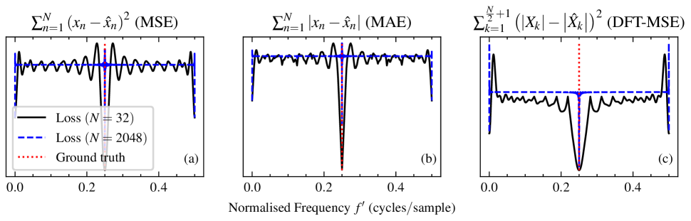
Fig. 1: The (a) mean squared error, (b) mean absolute error, and (c) DFT modulus mean squared error loss computed between two sinusoidal signals ($N=32$ and $N=2048$) as a function of the predicted frequency. Spectral leakage results in local minima across the full parameter range at lower $N$, while higher $N$ reveals the lack of informative frequency gradient, preventing effective first order optimization.

We are concerned with modelling the class of discrete-time signals that can be expressed as:

$$x_{n}=v_{n}+\sum_{k\in K}\alpha_{k}\cos\left(\omega_{k}n+\phi_{k}\right),$$ (1)

where $v_{n}\sim\mathcal{N}\left(0,\sigma^{2}\right)$, and $\alpha_{k},\omega_{k},\phi_{k}$ are the amplitude, frequency, and phase parameters, respectively, of unordered sinusoidal components with index set $K\subseteq\mathbb{N}$. Following the standard ML derivations, finding estimates $\hat{\alpha}_{k}$, $\hat{\omega}_{k}$, $\hat{\phi}_{k}$ is equivalent to minimizing the mean squared error of the model. In many applications of machine learning to audio, we are concerned with other formulations of the error. These can be accounted for by expressing the likelihood in terms of other signal representations, such as the discrete Fourier transform (DFT).

It is well established that when $\omega_{k}$ and $\phi_{k}$ are known, this problem is linear in $\alpha_{k}$ [22] – a property which, for example, allows DDSP models to directly predict harmonic amplitudes [14]. When $\phi$ is unknown, an optimal estimate can be found by evaluating the DTFT at the known frequencies $\omega_{k}$. In the case where frequency is unknown, however, the optimization problem is more challenging. Substituting Eqn. 1 into the mean squared error, for example, it is clear that the minimization objective is highly non-convex (as illustrated in Fig. 1), consisting of a sum of second order intermodulation products.

As only the global minimum represents a viable model fit, such a loss surface is problematic for gradient based optimizers: unless parameter estimates are initialized in the main basin of the function, optimization will converge on an incorrect solution. Further, as Turian & Henry [20] note, the gradient of audio loss functions is generally uninformative with respect to frequency. This is intuitive, considering the orthogonality of sinusoids on an infinite time horizon. As $N\to\infty$, the ripple reduces in magnitude until, in the limit, the loss is zero when $\hat{\omega}=\omega$ and constant for all other $\hat{\omega}$. The effect of increasing $N$ is illustrated in blue in Fig. 1.

2.1 Complex exponential surrogate

Our proposed technique circumvents these issues by defining a surrogate for a differentiable sinusoidal model. The surrogate produces an exponentially decaying sinusoid as the real part of an exponentiated complex number:

$$\mathfrak{s}_{n}(z_{k})\triangleq\mathfrak{Re}\left(z_{k}^{n}\right) =\left|z_{k}\right|^{n}\cos n\angle z_{k}$$ (2)

where $Z=\left\{z_{k}\in\mathbb{C}\mid k\in K\right\}$ is a set of specific surrogate parameters with index set $K$. As the surrogate maps $\mathfrak{s}_{n}\colon\mathbb{C}\to\mathbb{R}$ it does not have a complex derivative. However, its partial derivatives can be computed using Wirtinger’s calculus. A detailed explanation of these operators is beyond the scope of this paper, but we refer the interested reader to the work of Kreuz-Delgado [23] for an introduction. For present purposes, the conjugate Wirtinger derivative of the surrogate is:

$$\begin{split}\frac{\partial}{\partial\bar{z}}\mathfrak{s}_{n}(z)&=\frac{1}{2}\left(\frac{\partial}{\partial x}+j\frac{\partial}{\partial y}\right)\mathfrak{s}_{n}(z)=\frac{n}{2}\bar{z}^{n-1}\\ \end{split}$$ (3)

for $z=x+jy$. Where $\mathcal{L}$ is the loss between a signal produced by $\mathfrak{s}$ and a target, $-\frac{\partial\mathcal{L}}{\partial\bar{z}}$ is then the direction of steepest descent [23]. Unlike the frequency parameter of a real sinusoid, the surrogate parameter allows both the frequency and amplitude decay of the signal to be varied. As illustrated in Fig. 2, an optimizer can thus move the parameter inside the unit circle, creating an exponential amplitude decay, before moving it back out at the correct angle from the real line.

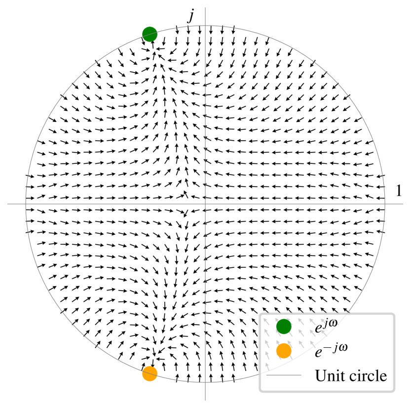
Fig. 2: Directions of negative Wirtinger conjugate derivatives $\frac{\partial\mathcal{L}_{\text{MSE}}}{\partial\bar{z}}$ displayed on the complex plane, where $\mathcal{L}_{\text{MSE}}$ is the mean-squared error taken with a single sinusoid of target frequency $\omega$. Arrows point in the direction of steepest descent. Our approach uses the Wirtinger differential operator with a complex exponential as a surrogate for a sinusoidal oscillator to allow frequency estimation in a differentiable signal processing framework.

The frequency estimate represented by the minimum is given by the complex argument of the surrogate parameter $\omega^{\ast}_{k}=\angle z_{k}^{\ast}$, where $Z^{\ast}=\left\{z_{k}^{\ast}\in\mathbb{C}\mid k\in K\right\}$ minimizes the loss:

$$Z^{\ast}=\arg\min_{Z}\sum_{n=1}^{N}\left(x_{n}-\sum_{k\in K}\mathfrak{s}_{n}\left(z_{k}\right)\right)^{2}$$ (4)

It follows that when target amplitudes $\alpha_{k}=1$, this gives $|z^{\ast}_{k}|=1$ and $\angle z^{\ast}_{k}=\omega_{k}$, which is equivalent to the ML estimate for frequency. In other cases, a linear amplitude parameter $\hat{\alpha}_{k}$ can be introduced to the surrogate, i.e. $\hat{\alpha}_{k}\mathfrak{s}_{n}\left(z_{k}\right)$. In this way, $\omega_{k}^{\ast}$ can give the ML estimate when $\alpha_{k}\neq 1$ and $\alpha_{k}$ is known, by simply setting $\hat{\alpha_{k}}=\alpha_{k}$. In the case where target amplitudes are unknown, $\hat{\alpha}_{k}$ can be learned jointly with surrogate parameters.

2.1.1 Amplitude estimation

Even when an amplitude coefficient is jointly learned, the complex exponential surrogate and the standard sinusoid may differ in the evolution of their amplitudes across time. However, assuming $z^{\ast}_{k}$ minimizes the least squares objective, we can recover an amplitude estimate by solving the opposite least squares problem. Specifically, to recover amplitudes from a surrogate model consisting of $|K|$ components $z_{k}$, we define $U\in\mathbb{R}^{N\times K}$ where $u_{nk}=\cos\angle z_{k}n$ and $\mathbf{v}\in\mathbb{R}^{N}$ where $\mathbf{v}=\sum_{k=1}^{K}\mathfrak{s}_{n}\left(z_{k}\right)$. For some linear signal representation $h\colon\mathbb{R}^{N}\to\mathbb{R}^{M}$, such as the identity mapping or a projection into a Fourier basis, the amplitude estimate is given by the ordinary least squares solution:

$$\mathbf{\alpha}^{\ast}=\left(H(U)^{T}H(U)\right)^{-1}H(U)^{T}h\left(\mathbf{v}\right),$$ (5)

where $H\colon\mathbb{R}^{N\times K}\to\mathbb{R}^{M\times K}$ applies $h$ to each column of a matrix. In practice, we may wish to select a nonlinear $h$ (e.g. the modulus of the DFT), leading to a nonlinear least squares problem. However, when the nonlinear solution is reasonably well approximated by the linear solution for values of $|z_{k}^{\ast}|$ close to $1$, jointly learning the amplitude factor and multiplying $\hat{\alpha}_{k}\alpha_{k}^{\ast}$ appears to yield acceptable estimates.

3 Evaluation

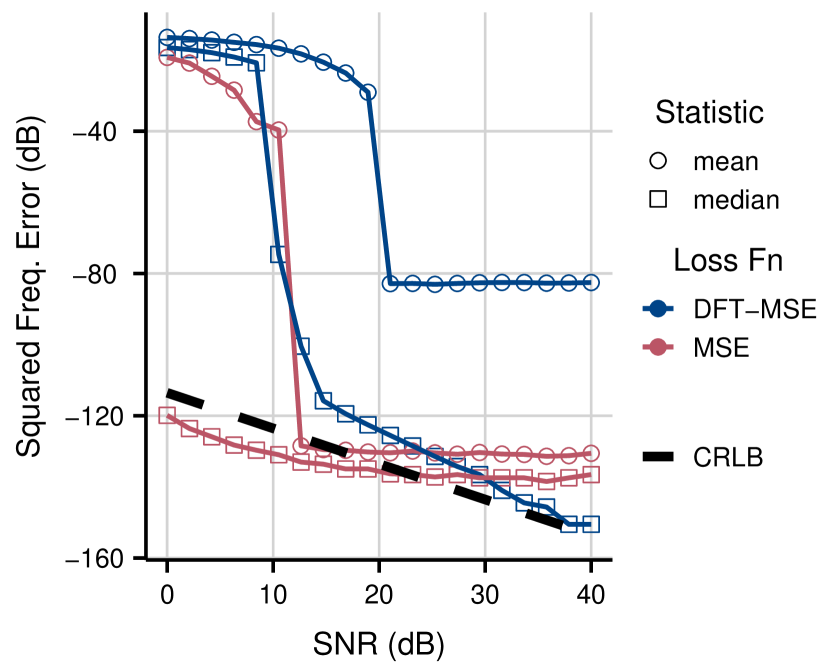
Fig. 3: The results of sinusoidal frequency estimation by gradient descent for a single sinusoid in Gaussian white noise, using both DFT magnitude mean squared error (DFT-MSE) and time-domain mean squared error (MSE). Both mean and median squared error are plotted for each experiment. Also plotted for reference is the Cramér-Rao lower bound (CRLB) on unbiased frequency estimators.

The performance of the surrogate model as a sinusoidal parameter estimator was evaluated by fitting the model to sinusoidal signals by gradient descent. All signals were of length $N=4096$.

3.1 Single sinusoid frequency estimation

In the single sinusoid case, we generated target signals with fixed amplitude $\alpha=1$ and initial phase $\phi=0$. The frequency parameter was sampled at 100 equal steps in the interval $[0.1\pi,0.9\pi]$, and the signal-to-noise ratio (SNR) at 20 steps in the interval $[0,40]$ dB, for a total of 2000 targets. The corresponding signals were synthesized using the real valued sinusoidal model in Eqn 1. A single starting parameter estimate was uniformly sampled from within the unit circle used for all 2000 targets, and the procedure was repeated with 10 different pseudo-random number generator seeds. Optimization proceeded for 50k steps using the Adam optimizer with a learning rate of $0.0001$ and the mean squared error loss on either the time-domain signal or DFT magnitude spectrum.

Fig. 3 displays the results of this experiment. The mean and median squared error between the predicted and ground truth frequency parameters are plotted on a decibel scale (i.e. $10\log_{10}(\text{MSE})$). The dotted black line plots the Cramér-Rao lower bound (CRLB) on variance for an unbiased estimator of sinusoidal frequency in Gaussian white noise, as given by Kay [1]. Whilst enquiry into the convergence properties of our method – and therefore the underlying bias of the estimator – is beyond the scope of this paper, this bound is representative of the performance of other sinusoidal parameter estimation algorithms. We thus plot it here to facilitate comparison and to illustrate that the surrogate model with time domain MSE loss is capable of achieving an error comparable with non-gradient based estimators.

We note that the mean squared error of the frequency domain loss (DFT-MSE) does not fall below roughly $-83$dB, but the median squared error continues to fall, implying an increasingly skewed error distribution as the SNR rises. We speculate that this occurs due to the loss of phase information in taking the modulus of the spectrum, and will investigate this hypothesis in future work.

3.2 Multi-sinusoid frequency and amplitude estimation

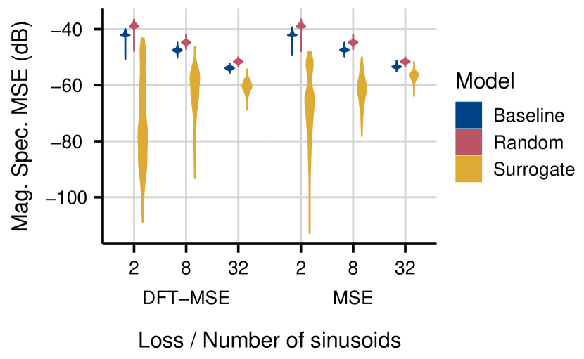
Fig. 4: Violin plots of the results of sinusoidal frequency and amplitude estimation by gradient descent for mixtures of $|K|\in\{2,8,32\}$ sinusoids, using both DFT magnitude (DFT-MSE) and time-domain (MSE) mean squared error losses. Plots represent the distribution of mean squared errors between magnitude spectra across 2000 runs.

In the multi-sinusoid case, targets were generated with phase $\phi_{k}=0$, and frequency and amplitude sampled from uniform distributions, $\omega_{k}\sim\mathcal{U}(0.1\pi,0.9\pi)$ and $\alpha_{k}\sim\mathcal{U}(0.1,1.0)$. 2000 sets of target parameters were sampled, and the corresponding signals synthesized using the real valued sinusoidal model. A random set of starting surrogate parameter estimates was uniformly sampled from the unit circle for each target, and linear amplitude was initialized for each component at $\hat{\alpha}_{k}=\frac{1}{|K|}$. The experiment was repeated for $|K|\in\left\{2,8,32\right\}$. Optimization ran for 100k steps using the same optimizer and losses. As a baseline, the same procedure was applied, using the same targets and starting estimates, to a differentiable real valued sinusoidal model.

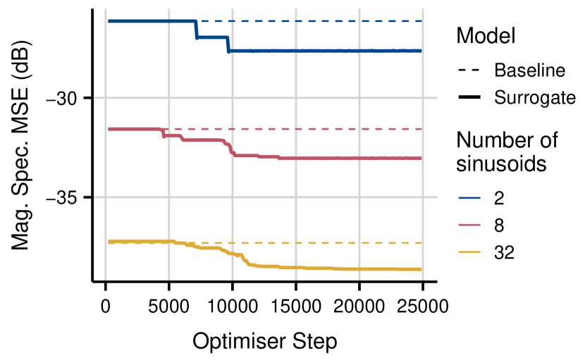
Fig. 5: The mean squared error between estimated and target magnitude spectra, evaluated at every 100th optimizer step for baseline and surrogate models trained with time-domain MSE loss with $|K|\in\{2,8,32\}$.

Fig. 4 displays the results of the experiment described in section 3.2. We plot the distributions of mean squared errors between target and predicted magnitude spectra using a dB scale for both our surrogate model and the real sinusoidal model baseline. For comparison, we also plot the errors achieved with randomly sampled sinusoidal parameters. Here, as expected, the surrogate clearly achieves superior performance, outperforming the baseline in all configurations.

We note that the performances of both the baseline and randomly sampled parameters improve as the number of components increases. We speculate that this effect is due to the proportionally smaller expected distance between each model component and any target component for higher values of $|K|$. Indeed, the decrease observed in the metric for both the baseline and random models is almost exactly proportional to the increase in the number of components – that is, on the decibel scale we observe a change of $10\log_{10}\frac{1}{4}\approx-6.02$ for a $4\times$ increase in components.

Conversely, the surrogate model’s performance slightly degrades as $|K|$ increases. Through informal observation of converged models, we hypothesize that this occurs due to a greater number of a specific class of local minimum, wherein multiple model components combine to match a single component in the target signal. We leave formal study of this behaviour to future work, but note that this phenomenon seems to predominantly occur only at the expense of quieter signal components.

To illustrate the optimization dynamics of the surrogate, Fig. 5 plots the evolution of the metric throughout optimization for both the surrogate and baseline model for a randomly selected set of target parameters. Here we see that the baseline metric either does not fall, or falls imperceptibly, as should be expected given the properties described in Section 2. The surrogate metric, however, does clearly fall before converging on a final value. It appears to solve the multi-sinusoid problem sequentially – that is, it seems to resolve each component one-by-one, causing the metric to fall to a series of plateaus. This observation may have implications for training strategies in DDSP deep learning tasks, where a plateau in a metric is typically taken as a signifier that a model has converged.

4 Conclusion

This work presented a technique for matching the frequency and amplitude parameters of a single- and multi-component sinusoidal model to a target signal by gradient descent. We evaluated the performance of our method on single and multiple sinusoid signals and demonstrated that it clearly outperforms a standard sinusoidal model in the multi-sinusoid case, whilst approaching the performance of other, non-gradient based estimators in the single sinusoid case.

This problem was previously intractable using differentiable signal processing techniques, preventing a variety of applications of this family of methods, including the modelling of inharmonic audio signals, unsupervised fundamental frequency detection, and more. Our approach now paves the way for these applications to be explored. In particular, we believe our surrogate model is suitable for use as a drop-in replacement for a differentiable sinusoidal model, and in future work will explore its capabilities in end-to-end learning with differentiable signal processing. We will also conduct further study into the surrogate model’s optimization characteristics.

References

- [1] Steven Kay, Fundamentals of Statistical Signal Processing: Estimation Theory, vol. 1, Pearson, 1st edition, May 1993.
- [2] P. Stoica, R.L. Moses, B. Friedlander, and T. Soderstrom, “Maximum likelihood estimation of the parameters of multiple sinusoids from noisy measurements,” IEEE Transactions on Acoustics, Speech, and Signal Processing, vol. 37, no. 3, pp. 378–392, Mar. 1989.
- [3] D. Rife and R. Boorstyn, “Single tone parameter estimation from discrete-time observations,” IEEE Transactions on Information Theory, vol. 20, no. 5, pp. 591–598, Sept. 1974.
- [4] T. Abatzoglou, “A fast maximum likelihood algorithm for frequency estimation of a sinusoid based on Newton’s method,” IEEE Transactions on Acoustics, Speech, and Signal Processing, vol. 33, no. 1, pp. 77–89, Feb. 1985.
- [5] D. C. Rife and R. R. Boorstyn, “Multiple Tone Parameter Estimation From Discrete-Time Observations,” Bell System Technical Journal, vol. 55, no. 9, pp. 1389–1410, Nov. 1976.
- [6] Saman S. Abeysekera, “Least-Squares Multiple Frequency Estimation using Recursive Regression Sum of Squares,” in 2018 IEEE International Symposium on Circuits and Systems (ISCAS), May 2018, pp. 1–5.
- [7] S. Parthasarathy and D.W. Tufts, “Maximum-likelihood estimation of parameters of exponentially damped sinusoids,” Proceedings of the IEEE, vol. 73, no. 10, pp. 1528–1530, 1985.
- [8] Fan-Shuo Tseng, Mantsawee Sanpayao, Tsang-Yi Wang, and Ming-Xian Zhong, “Low-Complexity High-Resolution Frequency Estimation of Multi-Sinusoidal Signals,” IEEE Transactions on Instrumentation and Measurement, vol. 71, pp. 1–12, 2022, Conference Name: IEEE Transactions on Instrumentation and Measurement.
- [9] P. Vishnu and C.S. Ramalingam, “An Improved LSF-based Algorithm for Sinusoidal Frequency Estimation that Achieves Maximum Likelihood Performance,” in 2020 International Conference on Signal Processing and Communications (SPCOM), Bangalore, India, July 2020, pp. 1–5, IEEE.
- [10] Y. Bresler and A. Macovski, “Exact maximum likelihood parameter estimation of superimposed exponential signals in noise,” IEEE Transactions on Acoustics, Speech, and Signal Processing, vol. 34, no. 5, pp. 1081–1089, Oct. 1986.
- [11] Vladislav S. Gromov, Alexey A. Vedyakov, Anastasiia O. Vediakova, Alexey A. Bobtsov, and Anton A. Pyrkin, “First-order frequency estimator for a pure sinusoidal signal,” in 2017 25th Mediterranean Conference on Control and Automation (MED), July 2017, pp. 7–11, ISSN: 2473-3504.
- [12] Anastasiia O. Vediakova, Alexey A. Vedyakov, Anton A. Pyrkin, Alexey A. Bobtsov, and Vladislav S. Gromov, “Finite Time Frequency Estimation for Multi-Sinusoidal Signals,” European Journal of Control, vol. 59, pp. 38–46, May 2021.
- [13] R. Kumaresan, L. Scharf, and A. Shaw, “An algorithm for pole-zero modeling and spectral analysis,” IEEE Transactions on Acoustics, Speech, and Signal Processing, vol. 34, no. 3, pp. 637–640, June 1986.
- [14] Jesse Engel, Lamtharn (Hanoi) Hantrakul, Chenjie Gu, and Adam Roberts, “DDSP: Differentiable Digital Signal Processing,” in 8th International Conference on Learning Representations, Addis Ababa, Ethiopia, Apr. 2020.
- [15] Ben Hayes, Charalampos Saitis, and György Fazekas, “Neural Waveshaping Synthesis,” in Proceedings of the 22nd International Society for Music Information Retrieval Conference, Online, Nov. 2021.
- [16] Franco Caspe, Andrew McPherson, and Mark Sandler, “DDX7: Differentiable FM Synthesis of Musical Instrument Sounds,” Aug. 2022, arXiv:2208.06169 [cs, eess].
- [17] Shahan Nercessian, Andy Sarroff, and Kurt James Werner, “Lightweight and Interpretable Neural Modeling of an Audio Distortion Effect Using Hyperconditioned Differentiable Biquads,” in ICASSP 2021 - 2021 IEEE International Conference on Acoustics, Speech and Signal Processing (ICASSP), Toronto, ON, Canada, June 2021, pp. 890–894, IEEE.
- [18] Christian J Steinmetz, Nicholas J Bryan, and Joshua D Reiss, “Style Transfer of Audio Effects with Differentiable Signal Processing,” J. Audio Eng. Soc., vol. 70, no. 9, pp. 14, 2022.
- [19] Joseph T. Colonel, Christian J. Steinmetz, Marcus Michelen, and Joshua D. Reiss, “Direct Design of Biquad Filter Cascades with Deep Learning by Sampling Random Polynomials,” in ICASSP 2022 - 2022 IEEE International Conference on Acoustics, Speech and Signal Processing (ICASSP), May 2022, pp. 3104–3108.
- [20] Joseph Turian and Max Henry, “I’m Sorry for Your Loss: Spectrally-Based Audio Distances Are Bad at Pitch,” arXiv:2012.04572 [cs, eess], Dec. 2020, arXiv: 2012.04572.
- [21] Jesse Engel, Rigel Swavely, and Adam Roberts, “Self-supervised Pitch Detection by Inverse Audio Synthesis,” in Proceedings of the International Conference on Machine Learning, 2020, p. 9.
- [22] Julius O. Smith, Spectral Audio Signal Processing, W3K Publishing, 2011.
- [23] Ken Kreutz-Delgado, “The Complex Gradient Operator and the CR-Calculus,” June 2009, arXiv:0906.4835 [math].