Redshift-evolutionary X-Ray and UV luminosity relation of quasars from Gaussian copula

Abstract

We construct a three-dimensional and redshift-evolutionary X-ray and ultraviolet ($L_{X}-L_{UV}$) luminosity relation for quasars from the powerful statistic tool called copula, and find that the constructed $L_{X}-L_{UV}$ relation from copula is more viable than the standard one and the observations favor the redshift-evolutionary relation more than $3\sigma$. The Akaike and Bayes information criterions indicate that the quasar data support strongly the three-dimensional $L_{X}-L_{UV}$ relation. Our results show that the quasars can be regarded as a reliable indicator of the cosmic distance if the $L_{X}-L_{UV}$ relation from copula is used to calibrate quasar data.

1 Introduction

Quasars (quasi-stellar objects, QSOs) are the extremely luminous persistent sources in the universe. They are found in the centers of some galaxies and powered by gas spiraling at high velocity into an extremely large black hole. The most powerful quasars have luminosities thousands of times greater than that of the Milky Way, and thus quasars can be visible at the very remote distance. The redshift of a quasar can reach $z>7$ (Mortlock et al., 2011; Bañados et al., 2018; Wang et al., 2021). Today, more than half a billion quasars have been identified by observations (Lyke et al., 2020). If quasars can be regarded as standard candles for probing the cosmic evolution, they can cover effectively the redshift desert of the cosmic observational data. Thus, quasars can help us to understand the properties of dark energy and the possible origin of the present Hubble constant ($H_{0}$) tension.

Properties of quasars have been proposed as probes to explore the cosmic expansion. These include quasar angular size measurements (Paragi et al., 1999; Chen & Ratra, 2003; Cao et al., 2017; Ryan et al., 2019; Cao et al., 2020, 2021), the anticorrelation between UV emission lines and luminosity (Baldwin, 1977; Osmer & Shields, 1999), the luminosity-mass relation in super-Eddington accreting quasars (Wang et al., 2014), the relation between luminosity and X-ray variability (La Franca et al., 2014) and the radius-luminosity relationship (Watson et al., 2011; Melia, 2014; Kilerci Eser et al., 2015).

The nonlinear relation between the X-ray luminosity and ultraviolet (UV) luminosity ($L_{X}-L_{UV}$) in quasars has been constructed to derive the distance of quasars and to build a quasar Hubble diagram up to $z\sim 7$ (Risaliti & Lusso, 2015, 2019; Lusso & Risaliti, 2016, 2017; Lusso et al., 2020). The $L_{X}-L_{UV}$ relation has been used widely in quasar cosmology (Lusso et al., 2019; Wei & Melia, 2020; Khadka & Ratra, 2020a, b, 2021; Lian et al., 2021; Li et al., 2021; Bargiacchi et al., 2021; Hu & Wang, 2022). Risaliti & Lusso (2019) found that there is a larger than 4$\sigma$ tension between the 1598 quasar data sets and the standard spatially-flat $\Lambda$CDM model with $\Omega_{\mathrm{m0}}=0.3$, where $\Omega_{\mathrm{m0}}$ is the present dimensionless matter density parameter. This may be a sign that quasars cannot be treated as the standard candle if the $L_{X}-L_{UV}$ relation is used (Khadka & Ratra, 2020b) and there have already been some discussions and controversies about this (Yang et al., 2020; Banerjee et al., 2021; Dainotti et al., 2022; Singal et al., 2022; Petrosian et al., 2022; Li et al., 2022). Furthermore, some data show evidence of redshift evolution of the X-ray and UV correlation (Khadka & Ratra, 2022), although recently Sacchi et al. (2022) found that this correlation still holds at $z>2.5$ by performing a one-by-one analysis of a sample of 130 quasars with high-quality X-ray and UV spectroscopic observations. Therefore, it remains interesting to research the possible redshift evolution of the $L_{X}-L_{UV}$ relation.

Copula is a powerful tool developed in modern statistics to describe the correlation between multivariate random variables (Nelsen, 2007)), and it has been used widely in various areas such as finance and hydrology. In recent years, copula has gradually been recognized by the astronomical community as an important tool to analyze data. For example, copula have been used to determine the luminosity function of the radio cores in the active galactic nucleus (Yuan et al., 2018), construct a period-mass function for extrasolar planets (Jiang et al., 2009), and build the correlation between the gamma ray burst (GRB) peak energy and the associated supernova peak brightness (Koen, 2009) and a new approximation for the low multipole likelihood of the cosmic microwave background (CMB) temperature (Benabed et al., 2009). Furthermore, copula has been introduced to research the convergence power spectrum from the weak lensing surveys (Sato et al., 2010, 2011), the gravitational-wave astronomy (Adamcewicz & Thrane, 2022), the galaxy luminosity functions (Takeuchi, 2010; Takeuchi et al., 2013; Takeuchi & Kono, 2020) and the large-scale structure fields of matter density (Scherrer et al., 2010; Qin et al., 2020). Recently, copula is used successfully in gamma ray burst (GRB) cosmology and gives an improved Amati correlation of GRBs (Liu et al., 2022a). Utilizing this improved Amati correlation to calibrate GRBs, the GRB data can give cosmological results, which are consistent with what were obtained from other popular data (Liu et al., 2022b).

Thus, we expect that copula may also play an important role in constructing the relations of quasars. In this work, we aim to construct, by using the powerful statistical tool copula, a three-dimensional $L_{X}-L_{UV}$ relation, which contains a redshift-dependent term. From the three-dimensional Gaussian copula, we obtain a three-dimensional and redshift-evolutionary $L_{X}-L_{UV}$ relation. Comparing it with the standard $L_{X}-L_{UV}$ relation by using the latest X-ray and UV flux measurements data (Lusso et al., 2020) that contain 2421 data sets of measurements, we find that the addition of the redshift-dependent term improves the viability of the $L_{X}-L_{UV}$ correlation significantly.

The rest of the Paper is organized as follows. In Section 2, we introduce the Gaussian copula and construct a three-dimensional $L_{X}-L_{UV}$ relation by using the copula function. The comparisons between the three-dimensional and standard $L_{X}-L_{UV}$ relations are made in Section 3. Finally, the conclusions are summarized in Section 4.

2 Three-dimensional $L_{X}-L_{UV}$ relation from copula

2.1 Copula

Copula is proposed to describe the intercorrelation between statistical variables (Nelsen, 2007). It can join or “couple” multivariate distribution functions with one-dimensional marginal distribution functions. Supposing that there are three variables $x_{1}$, $x_{2}$ and $x_{3}$ with the marginal cumulative distribution functions (CDFs) being $F_{1}(x_{1})$, $F_{2}(x_{2})$ and $F_{3}(x_{3})$, respectively, the joint distribution function of these three variables can be described by using copula function $C$:

$$H(x_{1},x_{2},x_{3})=C(F_{1}(x_{1}),F_{2}(x_{2}),F_{3}(x_{3}))\,.$$ (1)

The key point of Eq. (1) is that by using copula one can model the dependence structure and the marginal distribution separately. In the following, we set $u_{i}=F_{i}(x_{i})$ ($i=1,2,3$) for simplifying the expressions. The joint probability density function (PDF) $h(x_{1},x_{2},x_{3})$ of $H(x_{1},x_{2},x_{3})$ can be obtained through

$$h(x_{1},x_{2},x_{3}) = \frac{\partial^{3}H(x_{1},x_{2},x_{3})}{\partial x_{1}\partial x_{2}\partial x_{3}}$$ (2)

$$= \frac{\partial^{3}C(u_{1},u_{2},u_{3})}{\partial u_{1}\partial u_{2}\partial u_{3}}\frac{\partial u_{1}}{\partial x_{1}}\frac{\partial u_{2}}{\partial x_{2}}\frac{\partial u_{3}}{\partial x_{3}}$$

$$= c(u_{1},u_{2},u_{3})f_{1}(x_{1})f_{2}(x_{2})f_{3}(x_{3})\,,$$

where $f_{i}(x_{i})$ ($i=1,2,3$) are the marginal PDFs of $F_{i}(x_{i})$, and $c(u_{1},u_{2},u_{3})$ is the density function of $C(F_{1}(x_{1}),F_{2}(x_{2}),F_{3}(x_{3}))$.

Two main copula families are elliptic copulas and Archimedean copulas. The Gaussian copula belongs to a type of elliptic copulas and has a symmetric tail correlation. Since the Gaussian copula is the simplest and it can be analyzed analytically in many cases, we choose the Gaussian copula in our discussion and then we have

$$C(u_{1},u_{2},u_{3};\bm{\theta})=\Psi_{3}\left[\Psi_{1}^{-1}(u_{1}),\Psi_{1}^{-1}(u_{2}),\Psi_{1}^{-1}(u_{3});\bm{\theta}\right],$$ (3)

where $\bm{\theta}$ denotes the parameters of the copula function, and $\Psi_{3}$ and $\Psi_{1}$ are the standard three-dimensional and one-dimensional Gaussian CDFs, respectively, which are defined as

$$\Psi_{3}\left(\phi_{1},\phi_{2},\phi_{3};\bm{\theta}\right) = \int_{-\infty}^{\phi_{1}}\int_{-\infty}^{\phi_{2}}\int_{-\infty}^{\phi_{3}}\frac{1}{\sqrt{(2\pi)^{3}\mathrm{det}(\Sigma)}}$$ (4)

$$\times \exp\left\{-\frac{1}{2}\left[(\hat{\phi}_{1},\hat{\phi}_{2},\hat{\phi}_{3})^{T}\Sigma^{-1}(\hat{\phi}_{1},\hat{\phi}_{2},\hat{\phi}_{3})\right]\right\}\mathrm{d}\hat{\phi}_{1}\mathrm{d}\hat{\phi}_{2}\mathrm{d}\hat{\phi}_{3}\,,$$

and

$$\Psi_{1}\left(\phi\right) = \frac{1}{2}\mathrm{erfc}\left(-\frac{\phi}{\sqrt{2}}\right).$$ (5)

Here

$$\phi_{i}\equiv\Psi_{1}^{-1}(u_{i})=-\sqrt{2}\,\mathrm{erfc}^{-1}\left(2u_{i}\right),$$ (6)

$\Sigma$ is the covariance matrix, which relates to the correlation coefficients $\bm{\theta}=\{\rho_{12},\rho_{13},\rho_{23}\}$ ($\Sigma_{ij}=\Sigma_{ji}=\rho_{ij},\Sigma_{ii}=1$), and $\mathrm{erfc}$ and $\mathrm{erfc}^{-1}$ are complementary error function and its inverse, respectively.

The density function of the Gaussian copula can be calculated through

$$c(u_{1},u_{2},u_{3};\bm{\theta}) = \frac{\partial^{3}\Psi_{3}\left[\Psi_{1}^{-1}(u_{1}),\Psi_{1}^{-1}(u_{2}),\Psi_{1}^{-1}(u_{3});\bm{\theta}\right]}{\partial u_{1}\partial u_{2}\partial u_{3}}$$ (7)

$$= \frac{1}{\sqrt{\mathrm{det}(\Sigma)}}\exp\left\{-\frac{1}{2}\left[\bm{\Psi}^{-1^{T}}\left(\Sigma^{-1}-\mathbf{I}\right)\bm{\Psi}^{-1}\right]\right\},$$

where $\bm{\Psi^{-1}}\equiv\{\Psi_{1}^{-1}(u_{1}),\Psi_{1}^{-1}(u_{2}),\Psi_{1}^{-1}(u_{3})\}$. Then, the conditional PDF of $x_{1}$ denotes the probability of variable $x_{1}$ when $x_{2}$ and $x_{3}$ are fixed, which can be expressed as:

$$f_{x_{1}}(x_{1}|x_{2},x_{3};\bm{\theta})=\frac{c(u_{1},u_{2},u_{3};\bm{\theta})f_{1}(x_{1})f_{2}(x_{2})f_{3}(x_{3})}{c(u_{2},u_{3};\rho_{23})f_{2}(x_{2})f_{3}(x_{3})}=\frac{c(u_{1},u_{2},u_{3};\bm{\theta})}{c(u_{2},u_{3};\rho_{23})}f_{1}(x_{1})\,.$$ (8)

When the variable $x_{i}$ ($i=1,2,3$) obeys the Gaussian distribution with the mean value being $\mu_{i}$ and the standard deviation $\sigma_{i}$, its CDF $u_{i}$ can be expressed by

$$u_{i}=\frac{1}{2}\mathrm{erfc}\left(-\frac{x_{i}-\mu_{i}}{\sqrt{2}\sigma_{i}}\right).$$ (9)

Thus, from the Eq. (6), one can obtain

$$\Psi_{1}^{-1}\left(u_{i}\right)=-\sqrt{2}~{}\mathrm{erfc}^{-1}(2u_{i})=-\sqrt{2}~{}\mathrm{erfc}^{-1}\left[2\times\frac{1}{2}\mathrm{erfc}\left(-\frac{x_{i}-\mu_{i}}{\sqrt{2}\sigma_{i}}\right)\right]=\frac{x_{i}-\mu_{i}}{\sigma_{i}}\,.$$ (10)

Combining Eqs. (7), (8), and (10), we can obtain

$$f_{x_{1}}(x_{1}|x_{2},x_{3};\bm{\theta})=\frac{1}{\sqrt{2\pi}\sigma_{x_{1}\mid x_{2},x_{3}}}\exp\left[-\frac{1}{2}S(x_{1},x_{2},x_{3};\bm{\theta})\right],$$ (11)

where $\sigma_{x_{1}\mid x_{2},x_{3}}$ is the standard deviation of $f_{x_{1}}$, and

$$S(x_{1},x_{2},x_{3};\bm{\theta})=\frac{\left[\left(\rho_{23}^{2}-1\right)\hat{x}_{1}+\left(\rho_{12}-\rho_{13}\rho_{23}\right)\hat{x}_{2}+\left(\rho_{13}-\rho_{12}\rho_{23}\right)\hat{x}_{3}\right]^{2}}{\left(\rho_{23}^{2}-1\right)\left(\rho_{12}^{2}+\rho_{13}^{2}+\rho_{23}^{2}-2\rho_{13}\rho_{23}\rho_{12}-1\right)\sigma_{1}^{2}\sigma_{2}^{2}\sigma_{3}^{2}}$$ (12)

with $\hat{x}_{i}\equiv(x_{i}-\mu_{i})/\sigma_{i}$. Since $x_{1}$ follows the Gaussian distribution, the maximum probability of $x_{1}$ can be obtained from $S(x_{1},x_{2},x_{3};\bm{\theta})=0$. Thus, we can achieve the relation between variables $x_{1}$, $x_{2}$ and $x_{3}$ by solving $S(x_{1},x_{2},x_{3};\bm{\theta})=0$, and find that the relation can be simplified to be

$$x_{1}=a+bx_{2}+cx_{3}\,,$$ (13)

where

$$a = \frac{\mu_{3}\left(\rho_{13}-\rho_{12}\rho_{23}\right)\sigma_{1}\sigma_{2}+\mu_{2}\left(\rho_{12}-\rho_{13}\rho_{23}\right)\sigma_{1}\sigma_{3}}{\left(\rho_{23}^{2}-1\right)\sigma_{2}\sigma_{3}}+\mu_{1}\,,$$

$$b = \frac{\left(\rho_{13}\rho_{23}-\rho_{12}\right)\sigma_{1}}{\left(\rho_{23}^{2}-1\right)\sigma_{2}}\,,\quad c=\frac{\left(\rho_{12}\rho_{23}-\rho_{13}\right)\sigma_{1}}{\left(\rho_{23}^{2}-1\right)\sigma_{3}}\,.$$ (14)

2.2 Three-dimensional $L_{X}-L_{UV}$ relation

Risaliti & Lusso (2015) have found that there is a nonlinear relation between the X-ray luminosity $L_{X}$ and UV luminosity $L_{UV}$ in observational data of quasars. The $L_{X}-L_{UV}$ relation has the form

$$\log(L_{X})=\beta+\gamma\log(L_{UV})\,,$$ (15)

where $\beta$ and $\gamma$ are two free parameters to be determined from the data, and $\log\equiv\log_{10}$. Expressing the luminosity in terms of the flux, one can obtain

$$\log(F_{X})=\beta^{\prime}(z)+\gamma\log(F_{UV})\,,$$ (16)

where $F_{X}$ and $F_{UV}$ are the X-ray and UV fluxes, respectively, and $\beta^{\prime}(z)=2(\gamma-1)\log(d_{L})+\beta+(\gamma-1)\log(4\pi)$. Here $d_{L}$ is the luminosity distance. We can fit parameters $\gamma$ and $\beta$ by using the quasar data, if a concrete cosmological model is chosen.

Now, we will use the copula function to construct the correlation between $L_{X}$, $L_{UV}$ and the redshift. First, we assume that both $\log(L_{X})$ and $\log(L_{UV})$ follow Gaussian distributions with the distributional functions being

$$f(x)=\frac{1}{\sqrt{2\pi}\sigma_{x}}e^{-\frac{(x-\bar{a}_{x})^{2}}{2\sigma_{x}^{2}}}\,,\quad f(y)=\frac{1}{\sqrt{2\pi}\sigma_{y}}e^{-\frac{(y-\bar{a}_{y})^{2}}{2\sigma_{y}^{2}}}\,.$$ (17)

Here $x=\log(L_{UV})$, $y=\log(L_{X})$, $\bar{a}_{x}$ and $\bar{a}_{y}$ represent the mean values, and $\sigma_{x}$ and $\sigma_{y}$ are the standard deviations. We have checked that these assumptions are very reasonable by performing a statistical distribution test (Cramér-von Mises test (Cramér, 1928; Von Mises, 1928)) on $x$ and $y$ based on the $\Lambda$CDM model. Then, the redshift distribution of quasars is considered. In the upper panel of Fig. 1 we show the probability density distribution of 2421 quasar data points (Lusso et al., 2020) in the redshift $z$ space, which satisfies the gamma distribution apparently. The probability density distribution is plotted by requiring that the total area enclosed by the curve and the $z$ axis is normalized to one. Thus, if the value of the vertical axis is $P$ at redshift $z$, the probability of the data in the redshift region $(z-\delta z,z+\delta z)$ is $2P\delta z$, where $\delta z$ is a very small variation and thus the value of the vertical axis in the redshift region $(z-\delta z,z+\delta z)$ can be regarded as constant. Since the log-transformation is a common way to transform the non-Gaussian distribution into the Gaussian one, we consider the $z_{*}$ space, where $z_{*}\equiv\ln(\bar{a}+z)$ with $\bar{a}$ being a constant and $\ln\equiv\log_{e}$, and find that the distribution of quasars can be described approximately by using a Gaussian distribution $f(z_{*})$, which is shown in the down panel of Fig. 1. Thus, $f(z_{*})$ has the form

$$f(z_{*})=\frac{1}{\sqrt{2\pi}\sigma_{z_{*}}}e^{-\frac{(z_{*}-\bar{a})^{2}}{2\sigma_{z_{*}}^{2}}}\,.$$ (18)

We obtain that $\bar{a}=5$ is a very good set after choosing some different values of $\bar{a}$ for comparison since it can lead to very consistent fitting results in the following analysis.

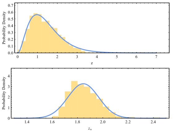
Figure 1: The histogram of 2421 quasar data points in the $z$ and $z_{*}$ spaces with the vertical axis representing the probability density. In the up and down panels, the solid lines represent the gamma distribution in the $z$ space and the Gaussian distribution in the $z_{*}$ space, respectively.

According to Eq. (13), we obtain the three-dimensional relation, which has the form

$$\log(L_{X})=\beta+\gamma\log(L_{UV})+\alpha\ln(\bar{a}+z)\,.$$ (19)

Apparently $\alpha$ is a new free parameter. Eq. (19) is different from the standard $L_{X}-L_{UV}$ relation (Eq. (15)) with the addition of a redshift-dependent term. When $\alpha=0$ the standard relation is recovered. When $\bar{a}=1$, our relation reduces to the one given in (Dainotti et al., 2022) obtained by assuming that the luminosities of quasars are corrected by a redshift dependent function $(1+z)^{\alpha}$. Converting the luminosity to the flux, one has

$$\log(F_{X}) = \Phi(\log(F_{UV}),d_{L})$$ (20)

$$= \beta^{\prime}+\gamma\log(F_{UV})+\alpha\ln(5+z)\,.$$

Eq. (20) is the main result of this Paper. In the following, we will discuss the viability of the three-dimensional $L_{X}-L_{UV}$ relation from copula.

3 relation test

In this section, we use two different methods (low-redshift calibration and simultaneous fitting) to test the viability of the three-dimensional $L_{X}-L_{UV}$ relation given in Eq. (20) and make a comparison between the three-dimensional and standard $L_{X}-L_{UV}$ relations.

3.1 Low-redshift calibration

Since $\beta^{\prime}$ is dependent on the luminosity distance $d_{L}$, we choose the fiducial cosmological model to give $d_{L}$. We consider two models: the specially flat $\Lambda$CDM with ($H_{0}=70~{}\mathrm{km~{}s^{-1}~{}Mpc^{-1}}$, $\Omega_{\mathrm{m0}}=0.3$) and with ($H_{0}=70~{}\mathrm{km~{}s^{-1}~{}Mpc^{-1}}$, $\Omega_{\mathrm{m0}}=0.4$), respectively. Since the furthest type Ia supernovae reaches to redshift $z\sim 2$ (Scolnic et al., 2018), we choose the quasar data within the low-redshift region $z<2$ to determine the values of the coefficients in the three-dimensional and standard $L_{X}-L_{UV}$ relations. Extrapolating these results to the high-redshift ($z>2$) data, we can obtain the Hubble diagram of high-redshift quasar data at $z\sim 7.5$. Finally, the high-redshift quasar data will be used to constrain the $\Lambda$CDM model. If the value of $\Omega_{\mathrm{m0}}$ assumed in the fiducial model is compatible with the one from the high-redshift data, the low-redshift and high-redshift data give consistent results and thus we regard this relation as viable and then the quasars can be taken as standard candles.

The data used in our analysis contain 2421 X-ray and UV flux measurements of quasars (Lusso et al., 2020), which cover the redshift range of $z\in[0.009,7.541]$. We use 1917 low-redshift data points for calibration. The values of the coefficients in the $L_{X}-L_{UV}$ relation can be obtained by minimizing $-\ln(\mathcal{L})$, where $\mathcal{L}$ is the D’Agostinis likelihood function (D’Agostini, 2005)

$$\mathcal{L} (\delta,\beta,\gamma,\alpha)\propto\prod_{i}\frac{1}{\sqrt{2\pi(\delta^{2}+\sigma_{i}^{2})}}\exp\left\{-\frac{[\log(F_{X})_{i}-\Phi(\log(F_{UV}),d_{L})_{i}]^{2}}{2\left(\delta^{2}+\sigma_{i}^{2}\right)}\right\}\,.$$ (21)

Here $\sigma_{i}$ represent the measurement errors in $\log(F_{X})$, $\delta$ is an intrinsic dispersion, function $\Phi$ is defined in Eq. (20), and $d_{L}$ is the luminosity distance predicted by the $\Lambda$CDM model, which is calculated as

$$d_{L}=(1+z)\frac{1}{H_{0}}\int_{0}^{z}{\frac{dz^{\prime}}{\sqrt{\Omega_{\mathrm{m0}}(1+z^{\prime})^{3}+(1-\Omega_{\mathrm{m0}})}}}\,.$$ (22)

In order to compare the three-dimensional $L_{X}-L_{UV}$ relation and the standard one, we use the Akaike information criterion (AIC) (Akaike, 1974, 1981) and the Bayes information criterion (BIC) (Schwarz, 1978), which are, respectively, defined as

$$\mathrm{AIC} = 2p-2\ln(\mathcal{L})\,,$$ (23)

$$\mathrm{BIC} = p\ln N-2\ln(\mathcal{L})\,,$$ (24)

where $p$ is the number of free parameters and $N$ is the number of data points. We need to calculate $\Delta$AIC(BIC) ($\Delta$AIC (BIC)$=$ AIC (BIC) $-$AIC_min (BIC_min)) of the two relations when comparing them. We have strong evidence against the relation that has a large AIC(BIC) if $\Delta\mathrm{AIC(BIC)}>10$ (Hu & Jeffreys, 1998).

The likelihood analysis is performed by using the Markov Chain Monte Carlo (MCMC) method as implemented in the $emcee$ package in $python$ 3.8 (Foreman-Mackey et al., 2013). Table 1 and Figure 2 show the results. From them, we can conclude that

• The value of $\alpha$ deviates from zero more than $3\sigma$, which indicates that the observational data support apparently the redshift-dependent luminosity relation.

• Since both $\Delta$AIC and $\Delta$BIC are larger than $20$, the three-dimensional relation from the copula function is favored strongly by the information criterions.

• The intrinsic dispersion has a negligible difference for all cases. And the values of $\beta$ are almost independent of the cosmological models.

Table 1: Marginalized one-dimensional best-fitting parameters with 1$\sigma$ confidence level from the low-redshift quasar data.

	$\Omega_{m0}$ = 0.3			$\Omega_{m0}$ = 0.4
	Standard	Three-Dimension		Standard	Three-Dimension
$\delta$	0.235(0.004)	0.232(0.004)		0.235(0.004)	0.232(0.004)
$\beta$	6.906(0.292)	7.502(0.302)		7.098(0.295)	7.606(0.305)
$\gamma$	0.645(0.010)	0.589(0.013)		0.638(0.010)	0.589(0.013)
$\alpha$	$-$	0.613(0.098)		$-$	0.544(0.096)
$-2\ln\mathcal{L}$	$-$32.483	$-$71.711		$-$39.661	$-$71.346
$\Delta$AIC	37.228	$-$		29.685	$-$
$\Delta$BIC	31.670	$-$		24.137	$-$

Note. — The values of $\sigma$ are in parentheses.

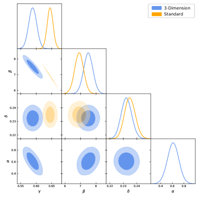
Figure 2: One-dimensional likelihood distributions and two-dimensional contours at 1$\sigma$ and 2$\sigma$ CLs. $\alpha$, $\beta$, and $\gamma$ are the coefficients of the luminosity relation and $\delta$ is the intrinsic dispersion. Left panel shows the result from the $\Lambda$CDM with $\Omega_{m0}=0.3$, and right panel shows the result from the $\Lambda$CDM with $\Omega_{m0}=0.4$. Blue and orange contours represent the three-dimensional and standard relations, respectively.

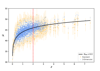
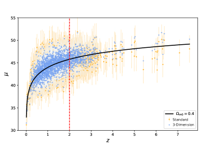
Figure 3: Hubble diagrams of quasars calibrated by low-redshift quasar data, which denotes the relation between the distance modulus $\mu$ and redshift $z$. The orange dots and the blue dots are derived from the standard relation and the three-dimensional and redshift-evolutionary one, respectively. The dashed red line corresponds to $z=2$.

Extrapolating the values of the coefficients of the luminosity relations and the intrinsic dispersion from the low-redshift data to the high-redshift samples, we can construct the Hubble diagram of quasars. The distance modulus and its errors are obtained from the formula given in the Appendix. In Fig. 3, the Hubble diagrams of quasars obtained from two different relations (standard and three dimension) and two different fiducial models are shown. Apparently, the distance modulus from the three-dimensional relation is closer to the theoretical curve than that from the standard relation.

We use the distance modulus of high-redshift quasars to constrain the $\Lambda$CDM model by minimizing $\chi^{2}$

$$\chi^{2}=\sum_{i=1}^{504}\left[\frac{\mu_{obs}\left(z_{i}\right)-\mu_{th}\left(z_{i}\right)}{\sigma_{\mu_{i}}^{obs}}\right]^{2}\,.$$ (25)

Here $\mu(z)=25+5\log\left[\frac{d_{L}(z)}{\mathrm{Mpc}}\right]$ is the distance modulus. The results are shown in Fig. 4 and summarized in Tab. 2. It is easy to see that the data from the three-dimensional relation can give a constraint on $\Omega_{\mathrm{m0}}$ consistent with that assumed in the fiducial model at the $1\sigma$ confidence level (CL), while the data from the standard relation cannot, and the deviations are larger than $3\sigma$. The AIC and BIC also favor strongly the three-dimensional relation. Therefore, we can conclude that the three-dimensional luminosity relation from copula is obviously superior to the standard relation. Using this three-dimensional relation, the quasars can be treated as the standard candle to probe the cosmic evolution.

To compare two relations with data more clearly, we plot the quasar data points in the $\log(L_{X})$-$\log(L_{UV})$ and $\log(L_{X})^{\prime}$-$\log(L_{UV})$ planes in Fig. 5, where $\log(L_{X})^{\prime}\equiv\log(L_{X})-\alpha\ln(z+5)$. The solid lines are luminosity relations calibrated by using the $\Lambda$CDM model with $\Omega_{m0}=0.3$ from the low-redshift data. It is easy to see that the three-dimensional and redshift-evolutionary relation is more consistent with the high-redshift data than the standard one.

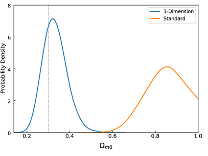
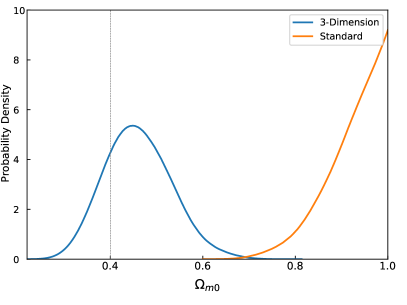
Figure 4: Constraint on $\Omega_{m0}$ of the $\Lambda$CDM model from the high-redshift quasar data. The vertical axis represents the probability density. The left and right panels represent the results from the $\Lambda$CDM model with $\Omega_{\mathrm{m0}}=0.3$ and $0.4$, respectively.

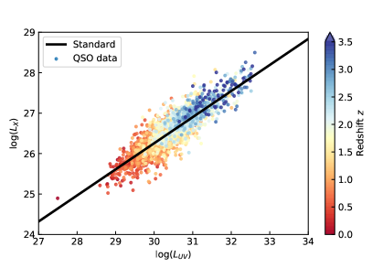
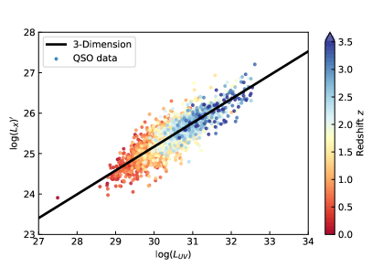
Figure 5: The comparison of the relations of $\log(L_{X})$-$\log(L_{UV})$ and $\log(L^{\prime}_{X})$-$\log(L_{UV})$ with quasar data points, where $\log(L_{X})^{\prime}=\log(L_{X})-\alpha\ln(z+5)$. The solid lines are luminosity relations calibrated by using the $\Lambda$CDM model with $\Omega_{m0}=0.3$ from the low-redshift quasar data.

Table 2: Marginalized one-dimensional best-fitting parameters with 1$\sigma$ CL from the high redshift quasar data.

Data set	Calibration	Relation	$\Omega_{m0}$	68%CL	$-2\ln\mathcal{L}$	$\Delta$AIC	$\Delta$BIC
High redshift	$\Omega_{m0}$ = 0.3	Standard	0.838	${}^{+0.110}_{-0.079}$	124.685	49.543	45.321
		Three-Dimension	0.326	${}^{+0.047}_{-0.063}$	73.142	$-$	$-$
	$\Omega_{m0}$ = 0.4	Standard	$>$0.902	$-$	123.011	48.399	44.177
		Three-Dimension	0.459	${}^{+0.063}_{-0.079}$	72.612	$-$	$-$

3.2 Simultaneous fitting

In the previous subsection, the fiducial cosmological model is used to study the reliability of the two different $L_{X}-L_{UV}$ relations. Here, we discard this condition. The coefficients of the relation and the cosmological parameters of $\Lambda$CDM model will be fitted simultaneously by minimizing the value of the D’Agostinis likelihood function (Eq. (21)).

Figure 6 shows one-dimensional probability density plots and contour plots of $\Omega_{\mathrm{m0}}$ and the coefficients of the two luminosity relations. The marginalized mean values with $1\sigma$ CL are summarized in Tab. 3. We find that the data favor apparently the redshift-evolutionary relation since $\alpha$ deviates from zero more than $3\sigma$. When the three-dimensional relation is used the quasar data can give an effective constraint on $\Omega_{\mathrm{m0}}$ ($\Omega_{\mathrm{m0}}=0.510^{+0.163}_{-0.254})$, which is consistent with what were given by the current popular data including type Ia supernova and the cosmic microwave background radiation and so on. However the quasar data only gives a lower bound limit on $\Omega_{\mathrm{m0}}$ for the standard relation. Furthermore, the AIC and BIC information criterions support strongly the three-dimensional relation since both $\Delta$AIC and $\Delta$BIC are larger than 50.

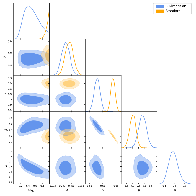
Figure 6: One-dimensional likelihood distributions and two-dimensional contours at 1$\sigma$ and 2$\sigma$ CLs from quasar data with the simultaneous fitting method. $\alpha$, $\beta$, and $\gamma$ are the coefficients of the luminosity relation, $\delta$ is the intrinsic dispersion and $\Omega_{m0}$ is the present dimensionless matter density parameter.

Table 3: Marginalized one-dimensional best-fitting parameters with 1$\sigma$ CL.

Relations	$\Omega_{m0}$	$\delta$	$\beta$	$\gamma$	$\alpha$	$-2\ln\mathcal{L}$	$\Delta$AIC	$\Delta$BIC
Standard	$>0.924$	$0.228^{+0.004}_{-0.004}$	$7.021^{+0.249}_{-0.249}$	$0.639^{+0.008}_{-0.008}$	$-$	$-109.566$	65.100	59.308
Three-Dimension	$0.510^{+0.163}_{-0.254}$	$0.225^{+0.004}_{-0.004}$	$7.825^{+0.316}_{-0.316}$	$0.579^{+0.011}_{-0.011}$	$0.580^{+0.084}_{-0.099}$	$-176.666$	$-$	$-$

4 Conclusions

Using the powerful statistic tool called copula, we construct a three-dimensional $L_{X}-L_{UV}$ relation of quasars, which contains an extra redshift-dependent term as opposed to the standard relation. We use two different methods to test the reliability of the relation from copula. One is to use the low-redshift quasar data to determine the values of relation coefficients after assuming the $\Lambda$CDM as the fiducial cosmological model, and extrapolate the results to the high-redshift data to give the Hubble diagram of quasars. Then these high-redshift data are used to constrain the $\Lambda$CDM model. By comparing the results from the high-redshift data with the ones given in the fiducial model, we can judge which relation is favored by quasar data. The other is to determine the coefficients of the luminosity relations and the cosmological parameters simultaneously from quasars. Two different methods give the same conclusion that the constraint on $\Omega_{\mathrm{m0}}$ from the three-dimensional $L_{X}-L_{UV}$ relation is more consistent with what was used in the fiducial cosmological model and obtained from other popular data than that from the standard relation. The observations favor a redshift-evolutionary $L_{X}-L_{UV}$ relation more than $3\sigma$. According to the AIC and BIC information criterions, we find that the quasar data support strongly the three-dimensional $L_{X}-L_{UV}$ relation. Our results indicate that quasars can be regarded as the reliable indicator of the cosmic distance if the three-dimensional $L_{X}-L_{UV}$ relation is used to calibrate quasar data.

Appendix A Distance modulus

The distance modulus $\mu(z)$ relates to the luminosity distance through

$$\mu(z)=25+5\log\left[\frac{d_{L}(z)}{\mathrm{Mpc}}\right]\,.$$ (A1)

Thus, if a cosmological model is assumed, the theoretical value of the distance modulus $\mu_{\mathrm{th}}(z)$ can be obtained easily. When the quasar data are considered, the observed value of the distance modulus $\mu_{\mathrm{obs}}(z)$ can be deduced from Eq (20) and Eq (A1) and has the form

$$\mu_{\mathrm{obs}}(z)=\frac{5}{2(\gamma-1)}\left[\log(F_{X})-\gamma\log(F_{UV})-\alpha\ln(5+z)-\beta^{\prime}\right]-97.447\,,$$ (A2)

where $\beta^{\prime}=\beta+(\gamma-1)\log(4\pi)$. Setting $y=\log(F_{X})$, $x=\log(F_{UV})$, one can get the error of the distance modulus by using the transfer formula

$$\sigma_{\mu}^{2} = \delta^{2}+\left(\frac{\partial\mu}{\partial\gamma}\right)^{2}\sigma_{\gamma}^{2}+\left(\frac{\partial\mu}{\partial\beta}\right)^{2}\sigma_{\beta}^{2}+\left(\frac{\partial\mu}{\partial\alpha}\right)^{2}\sigma_{\alpha}^{2}+\left(\frac{\partial\mu}{\partial y}\right)^{2}\sigma_{y}^{2}$$ (A3)

$$+ 2\sum_{i=1}^{4}\sum_{j=i+1}^{4}\left(\frac{\partial y(x;\bm{\bar{\theta}})}{\partial\bar{\theta}_{i}}\frac{\partial y(x;\bm{\bar{\theta}})}{\partial\bar{\theta}_{j}}\right)C_{ij}\,,$$

where $\bm{\bar{\theta}}=(\delta,\beta,\gamma,\alpha)$ and

$$\frac{\partial\mu}{\partial\gamma} = -\frac{\Gamma}{\gamma-1}\left[y-x-\alpha\ln(5+z)-\beta\right],$$

$$\frac{\partial\mu}{\partial\beta} = -\Gamma,\qquad\frac{\partial\mu}{\partial y}=\Gamma,\qquad\frac{\partial\mu}{\partial\alpha}=-\Gamma\ln(5+z)\,.$$ (A4)

Here $\Gamma=\frac{5}{2(\gamma-1)}$. In Eq. (A3), the covariance matrix can be approximately evaluated from

$$\left(C^{-1}\right)_{ij}\left(\bm{\bar{\theta}}\right)=\left.\frac{\partial^{2}\left[-\ln\mathcal{L}\left(\bm{\bar{\theta}}\right)\right]}{\partial\bar{\theta}_{i}\partial\bar{\theta}_{j}}\right|_{\bm{\bar{\theta}}=\bm{\bar{\theta}}_{0}}\,,$$ (A5)

where $\bm{\bar{\theta}}_{0}$ denote the best-fitted values. Substituting Eq. (A) into Eq. (A3), one has

$$\sigma_{\mu}^{2} = \delta^{2}+\left[\frac{\Gamma}{\gamma-1}\left(y-x-\alpha\ln(5+z)-\beta\right)\right]^{2}\sigma_{\gamma}^{2}+\Gamma^{2}\sigma_{\beta}^{2}+\Gamma^{2}\sigma_{y}^{2}$$ (A6)

$$+ \left[\Gamma\ln(5+z)\right]^{2}\sigma_{\alpha}^{2}+2\sum_{i=1}^{4}\sum_{j=i+1}^{4}\left(\frac{\partial y(x;\bm{\bar{\theta}})}{\partial\bar{\theta}_{i}}\frac{\partial y(x;\bm{\bar{\theta}})}{\partial\bar{\theta}_{j}}\right)C_{ij}\,.$$

References

- Adamcewicz & Thrane (2022) Adamcewicz, C. & Thrane, E. 2022, MNRAS, 517, 3928. doi: 10.1093/mnras/stac2961
- Akaike (1974) Akaike, H. 1974, ITAC, 19, 716
- Akaike (1981) Akaike, H. 1981, J. Eon., 16, 3, doi: 10.1016/0304-4076(81)90071-3
- Bañados et al. (2018) Bañados, E., Venemans, B. P., Mazzucchelli, C., et al. 2018, Nature, 553, 473, doi: 10.1038/nature25180
- Banerjee et al. (2021) Banerjee, A., Ó Colgáin, E., Sasaki, M., Sheikh-Jabbari, M, M., & Yang, T. 2021, Phys. Lett. B, 818, 136366, doi: 10.1016/j.physletb.2021.136366
- Baldwin (1977) Baldwin, J. A. 1977, ApJ, 214, 679, doi: 10.1086/155294
- Bargiacchi et al. (2021) Bargiacchi, G., Benetti, M., Capozziello, S., et al. 2022, MNRAS, 515, 1795. doi: 10.1093/mnras/stac1941
- Benabed et al. (2009) Benabed, K., Cardoso, J. F., Prunet, S., & Hivon, E. 2009, MNRAS, 400, 219, doi: 10.1111/j.1365-2966.2009.15202.x
- Cao et al. (2021) Cao, S., Ryan, J., Khadka, N., & Ratra, B. 2021, MNRAS, 501, 1520, doi: 10.1093/mnras/staa3748
- Cao et al. (2020) Cao, S., Ryan, J., & Ratra, B. 2020, MNRAS, 497, 3191, doi: 10.1093/mnras/staa2190
- Cao et al. (2017) Cao, S., Zheng, X., Biesiada, M., et al. 2017, A&A, 606, A15, doi: 10.1051/0004-6361/201730551
- Chen & Ratra (2003) Chen, G., & Ratra, B. 2003, ApJ, 582, 586, doi: 10.1086/344786
- Cramér (1928) Cramér, H. 1928, Scandinavian Actuarial Journal, 13, 74.
- D’Agostini (2005) D’Agostini, G. 2005, arXiv e-prints, physics/0511182. https://arxiv.org/abs/physics/0511182
- Dainotti et al. (2022) Dainotti, M. G., Bargiacchi, G., Lenart, A. Ł., et al. 2022, ApJ, 931, 106. doi: 10.3847/1538-4357/ac6593
- Foreman-Mackey et al. (2013) Foreman-Mackey, D., Conley, A., Meierjurgen Farr, W., et al. 2013, emcee: The MCMC Hammer, Astrophysics Source Code Library, record ascl:1303.002. http://ascl.net/1303.002
- Hu & Wang (2022) Hu, J. P. & Wang, F. Y. 2022, A&A, 661, A71. doi: 10.1051/0004-6361/202142162
- Hu & Jeffreys (1998) Jeffreys, H. 1998, The theory of probability (Oxford: Oxford Univ. Press)
- Jiang et al. (2009) Jiang, I.-G., Yeh, L.-C., Chang, Y.-C., & Hung, W.-L. 2009, AJ, 137, 329, doi: 10.1088/0004-6256/137/1/329
- Khadka & Ratra (2020a) Khadka, N., & Ratra, B. 2020a, MNRAS, 492, 4456, doi: 10.1093/mnras/staa101
- Khadka & Ratra (2020b) Khadka, N., & Ratra, B. 2020b, MNRAS, 497, 263, doi: 10.1093/mnras/staa1855
- Khadka & Ratra (2021) Khadka, N., & Ratra, B. 2021, MNRAS, 502, 6140, doi: 10.1093/mnras/stab486
- Khadka & Ratra (2022) Khadka, N., & Ratra, B. 2022, MNRAS, 510, 2753, doi: 10.1093/mnras/stab3678
- Kilerci Eser et al. (2015) Kilerci Eser, E., Vestergaard, M., Peterson, B. M., Denney, K. D., & Bentz, M. C. 2015, ApJ, 801, 8, doi: 10.1088/0004-637X/801/1/8
- Koen (2009) Koen, C. 2009, MNRAS, 393, 1370, doi: 10.1111/j.1365-2966.2008.14116.x
- La Franca et al. (2014) La Franca, F., Bianchi, S., Ponti, G., Branchini, E., & Matt, G. 2014, ApJ, 787, L12, doi: 10.1088/2041-8205/787/1/L12
- Li et al. (2021) Li, X., Keeley, R. E., Shafieloo, A., et al. 2021, MNRAS, 507, 919, doi: 10.1093/mnras/stab2154
- Li et al. (2022) Li, Z., Huang, L., & Wang, J. 2022, MNRAS, 517, 1901. doi: 10.1093/mnras/stac2735
- Lian et al. (2021) Lian, Y., Cao, S., Biesiada, M., et al. 2021, MNRAS, 505, 2111, doi: 10.1093/mnras/stab1373
- Liu et al. (2022a) Liu, Y., Chen, F., Liang, N., et al. 2022a, ApJ, 931, 50, doi: 10.3847/1538-4357/ac66d3
- Liu et al. (2022b) Liu, Y., Liang, N., Xie, X., et al. 2022b, ApJ, 935, 7, doi: 10.3847/1538-4357/ac7de5
- Lusso & Risaliti (2016) Lusso, E. & Risaliti, G. 2016, ApJ, 819, 154. doi: 10.3847/0004-637X/819/2/154
- Lusso & Risaliti (2017) Lusso, E. & Risaliti, G. 2017, A&A, 602, A79. doi: 10.1051/0004-6361/201630079
- Lusso et al. (2019) Lusso, E., Piedipalumbo, E., Risaliti, G., et al. 2019, A&A, 628, L4. doi: 10.1051/0004-6361/201936223
- Lusso et al. (2020) Lusso, E., Risaliti, G., Nardini, E., et al. 2020, A&A, 642, A150, doi: 10.1051/0004-6361/202038899
- Lyke et al. (2020) Lyke, B. W., Higley, A. N., McLane, J. N., et al. 2020, ApJS, 250, 8, doi: 10.3847/1538-4365/aba623
- Melia (2014) Melia, F. 2014, J. Cosmology Astropart. Phys, 2014, 027, doi: 10.1088/1475-7516/2014/01/027
- Mortlock et al. (2011) Mortlock, D. J., Warren, S. J., Venemans, B. P., et al. 2011, Nature, 474, 616, doi: 10.1038/nature10159
- Nelsen (2007) Nelsen, R. B. 2007, An introduction to copulas (New York: Springer)
- Osmer & Shields (1999) Osmer, P. S., & Shields, J. C. 1999, in Astronomical Society of the Pacific Conference Series, Vol. 162, Quasars and Cosmology, ed. G. Ferland & J. Baldwin, 235
- Paragi et al. (1999) Paragi, Z., Frey, S., Gurvits, L. I., et al. 1999, A&A, 344, 51. https://arxiv.org/abs/astro-ph/9901396
- Petrosian et al. (2022) Petrosian, V., Singal, J., & Mutchnick, S. 2022, ApJ, 935, L19. doi: 10.3847/2041-8213/ac85ac
- Qin et al. (2020) Qin, J., Yu, Y., & Zhang, P. 2020, ApJ, 897, 105. doi: 10.3847/1538-4357/ab952f
- Risaliti & Lusso (2015) Risaliti, G., & Lusso, E. 2015, ApJ, 815, 33, doi: 10.1088/0004-637X/815/1/33
- Risaliti & Lusso (2019) Risaliti, G., & Lusso, E. 2019, NatAs, 3, 272, doi: 10.1038/s41550-018-0657-z
- Ryan et al. (2019) Ryan, J., Chen, Y., & Ratra, B. 2019, MNRAS, 488, 3844, doi: 10.1093/mnras/stz1966
- Sacchi et al. (2022) Sacchi, A., Risaliti, G., Signorini, M., et al. 2022, A&A, 663, L7, doi: 10.1051/0004-6361/202243411
- Sato et al. (2010) Sato, M., Ichiki, K., & Takeuchi, T. T. 2010, Phys. Rev. Lett., 105, 251301. doi: 10.1103/PhysRevLett.105.251301
- Sato et al. (2011) Sato, M., Ichiki, K., & Takeuchi, T. T. 2011, Phys. Rev. D, 83, 023501. doi: 10.1103/PhysRevD.83.023501
- Scherrer et al. (2010) Scherrer, R. J., Berlind, A. A., Mao, Q., et al. 2010, ApJ, 708, L9. doi: 10.1088/2041-8205/708/1/L9
- Schwarz (1978) Schwarz, G. 1978, AnSta, 6, 461
- Scolnic et al. (2018) Scolnic, D. M., Jones, D. O., Rest, A., et al. 2018, ApJ, 859, 101
- Singal et al. (2022) Singal, J., Mutchnick, S., & Petrosian, V. 2022, ApJ, 932, 111. doi: 10.3847/1538-4357/ac6f06
- Takeuchi (2010) Takeuchi, T. T. 2010, MNRAS, 406, 1830. doi: 10.1111/j.1365-2966.2010.16778.x
- Takeuchi & Kono (2020) Takeuchi, T. T. & Kono, K. T. 2020, MNRAS, 498, 4365. doi: 10.1093/mnras/staa2558
- Takeuchi et al. (2013) Takeuchi, T. T., Sakurai, A., Yuan, F.-T., et al. 2013, EP&S, 65, 281. doi: 10.5047/eps.2012.06.008
- Von Mises (1928) Von Mises, R. 1928, Wahrscheinlichkeit, Statistik und Wahrheit (Wien: Springer)
- Wang et al. (2021) Wang, F., Yang, J., Fan, X., et al. 2021, ApJ, 907, L1, doi: 10.3847/2041-8213/abd8c6
- Wang et al. (2014) Wang, J.-M., Du, P., Hu, C., et al. 2014, ApJ, 793, 108, doi: 10.1088/0004-637X/793/2/108
- Watson et al. (2011) Watson, D., Denney, K. D., Vestergaard, M., & Davis, T. M. 2011, ApJ, 740, L49, doi: 10.1088/2041-8205/740/2/L49
- Wei & Melia (2020) Wei, J.-J. & Melia, F. 2020, ApJ, 888, 99, doi: 10.3847/1538-4357/ab5e7d
- Yang et al. (2020) Yang, T., Banerjee, A., & Ó Colgáin, E. 2020, Phys. Rev. D, 102, 123532, doi: 10.1103/PhysRevD.102.123532
- Yuan et al. (2018) Yuan, Z., Wang, J., Worrall, D. M., Zhang, B.-B., & Mao, J. 2018, ApJS, 239, 33, doi: 10.3847/1538-4365/aaed3b