Residual Back Projection With Untrained Neural Networks

Abstract

Background and Objective: The success of neural networks in a number of image processing tasks has motivated their application in image reconstruction problems in computed tomography (CT). While progress has been made in this area, the lack of stability and theoretical guarantees for accuracy, together with the scarcity of high-quality training data for specific imaging domains pose challenges for many CT applications. In this paper, we present a framework for iterative reconstruction (IR) in CT that leverages the hierarchical structure of neural networks, without the need for training. Our framework incorporates this structural information as a deep image prior (DIP), and uses a novel residual back projection (RBP) connection that forms the basis for our iterations.
Methods: We propose using an untrained U-net in conjunction with a novel residual back projection to minimize an objective function and achieve high-accuracy reconstruction. In each iteration, the weights of the untrained U-net are optimized, and the output of the U-net in the current iteration is used to update the input of the U-net in the next iteration through the aforementioned RBP connection.
Results: Experimental results demonstrate that the RBP-DIP framework offers improvements over other state-of-the-art conventional IR methods, as well as pre-trained and untrained models with similar network structures under multiple conditions. These improvements are particularly significant in the few-view, limited-angle, and low-dose imaging configurations.
Conclusions: Applying to both parallel and fan beam X-ray imaging, our framework shows significant improvement under multiple conditions. Furthermore, the proposed framework requires no training data and can be adjusted on-demand to adapt to different conditions (e.g. noise level, geometry, and imaged object).

1 Introduction

CT reconstruction algorithms are essential in a number of biomedical imaging applications. The traditional filtered back projection (FBP) algorithm is widely used in commercial scanners as it is computationally efficient. However, its image quality is heavily affected by deviations from ideal imaging conditions (e.g., low-dose, few-view, and limited-angle). To improve image quality in these imaging applications, iterative reconstruction (IR) methods leverage mathematical models for acquisition as well as image priors into an optimization process that forms the basis for image reconstruction [10]. They have been widely studied in CT imaging and are considered the gold standard, their performance in practical imaging applications, robustness, and image quality issues are well understood [35].

Neural network related methods have provided a new set of approaches in CT reconstruction. These methods can be used to improve image quality before (pre-processing, such as sinogram synthesis [18]), during (end-to-end reconstruction [46], plug in [23, 22]), or after (post processing, such as artifacts removal [39]) reconstruction. The successful application of neural network methods in CT reconstruction depends on the availability of high-quality training data and their ability to learn priors that can generalize to instances outside the training distribution. While deep learning methods have had a significant impact in CT imaging research [33], their application in reconstruction poses significant challenges as their lack of stability can lead to introduction of false structures (hallucinations) that may lead to detrimental effects in medical imaging [2, 6].

In this paper, a reconstruction framework that inherits the advantages of neural networks’ hierarchical structure and conventional IR methods is proposed. We leverage an untrained U-net, as a deep image prior (DIP), together with a novel residual back projection (RBP) connection that optimizes the weights to match the measurements. The input is updated iteratively by conventional IR algorithms through the newly introduced RBP connection during the reconstruction process. Since our RBP-DIP framework has no training process and does not require a training dataset, it eliminates the possibility of hallucinations. Furthermore, it benefits from the stability properties of traditional IR methods, facilitated by the introduction of the RBP connection. The experiments show that the RBP-DIP provides significant improvements over conventional methods and other neural network models (both untrained and pre-trained) with a similar network structure under both parallel-beam and fan-beam geometries. The observed improvements are most significant under few-view, limited-angle, and low-dose conditions.

The main advantages of the proposed RBP-DIP framework are as follows:

• No reliance on training data: the RBP-DIP algorithm employs an untrained neural network, thus deviates from conventional neural network methodologies. RBP-DIP aligns more closely with IR techniques as it directly minimizes the loss function on inference data. Consequently, the RBP-DIP algorithm needs no training data, therefore circumventing interferences commonly associated with training data and the training process.

• Integration of DIP and IR: Compared with conventional IR methods, the original DIP algorithm can generate better images when the corresponding inverse problem is highly ill-posed. However, such advantages diminish as the number of measurements increases. On the other hand, while IR algorithms suffer from severe artifacts under ill-posed conditions, their performance becomes stable with sufficient measurements. The RBP-DIP algorithm, through the RBP connection, seamlessly combines the strengths of both, achieving superior performance across various conditions.

The remainder of this paper is organized as follows: the details of the CT reconstruction problem and the related works are introduced in Section 2. The proposed framework is introduced in Section 3, and compared with conventional methods, pre-trained and untrained methods with a similar network structure on real CT images under various imaging conditions in Section 4. The results from our experiments are discussed in Section 5 followed by the conclusion Section 6.

2 Related Works

2.1 Iterative CT Reconstruction

IR approaches frame image reconstruction as an optimization problem, minimizing the inconsistency between the forward projection of the iterate and the measurements. X-ray physics, non-ideal effects, and image priors can be incorporated into the reconstruction algorithms by employing various constraints, regularizations, and forward models. The objective function for the CT optimization problem is often expressed by fidelity and regularization terms:

$$\boldsymbol{c}^{*}=\operatorname*{arg\,min}_{\boldsymbol{c}}||\boldsymbol{g}-\boldsymbol{A}\boldsymbol{c}||^{2}_{2}+\lambda R(\boldsymbol{c}),$$ (1)

where $\boldsymbol{c}$, $\boldsymbol{g}$, $\boldsymbol{A}$, and $R$ indicate the image coefficients, sinogram measurements, forward model, and regularization respectively. With accurate forward models [24, 25, 40] and effective priors [27, 16, 34, 11, 7, 42, 17], high-quality reconstruction imaging is possible under non-ideal conditions.

However, when the inverse problem is highly ill-posed (e.g., few-view and limited-angle), the generation of high-quality reconstruction results can be challenging when using hand-crafted priors such as sparsity-promoting regularizations, even in the absence of measurement noise. In that case, researchers proposed using application-specific priors that are learned from a sample of images to further improve the reconstruction accuracy. Multiple neural network related approaches are developed following this line of thought, and will be discussed in the next section.

2.2 CT Reconstruction Using Pre-Trained Neural Networks

The end-to-end approaches in image reconstruction learn a mapping from the acquisition data to the reconstructed images that can be employed in many imaging modalities as demonstrated by Zhu et al. [46]. However, the use of fully connected layers makes the computational costs necessary for reconstruction at practical resolutions unacceptable. To circumvent the use of fully connected layers, researchers proposed incorporating additional information into the input to simplify the task so that fully convolutional neural networks can be used for image reconstruction. This is demonstrated by Zhang et al. [41], Chen et al [8], and Ye et al. [37], who suggested utilizing back projections, filtered back projections, and single-view back projections as inputs for high-quality CT reconstruction, respectively.

Recently, more sophisticated models have been developed, which involve the collaboration of multiple neural networks working on various subtasks to achieve enhanced performance. Yin et al. [38] introduced an approach that employs two neural networks for denoising in both the sinogram and the image domain. Hu et al. [14] and Zhang et al. [43] extended this concept by incorporating three neural networks. In addition to the two denoising neural networks described in [38], an auxiliary image domain discriminator for real and reconstructed images was integrated to further refine the model. Similar architectures have also been explored in [36, 20].

To effectively leverage that many sub-networks, increasingly complex multi-loss functions are proposed. For instance, the multi-loss function in [43] contains five losses, four of which compare the differences between the denoised sinogram, FBP of the denoised sinogram, reconstructed image, sinogram of the reconstructed image, and their respective ground truth, while the fifth loss constitutes the loss function for the discriminator. Additional examples can be found in the works of Ma et al. [20] and Xie et al. [36]. The former employed three loss functions whereas the latter utilized four loss functions.

2.3 Challenges in Pre-Trained Neural Networks

Instability has been considered the greatest drawback for neural network image reconstruction. Neural network reconstruction algorithms are designed to learn the prior distribution of the imaged objects from training datasets implicitly or explicitly, so that high-quality reconstructions can be made even with limited and noisy measurements. However, the aforementioned circumstances are predicated upon the assumption that the inference data and training data follow the same distribution. This is particularly problematic for image reconstruction in the context of medical imaging as the learned network may omit patient-specific features and replace them with normal features learned from the training dataset. A number of studies have shown that deep learning reconstruction methods are inherently unstable, and features can be present in reconstructions that are hallucinated by the network, as investigated by Antun et al. [2] and Gottschling et al. [13].

Another problem is that current neural network related algorithms are difficult to implement on a large scale. On the one hand, practical neural networks are mostly challenging to train. For example, the multi-loss functions utilized in the aforementioned methods necessitate the introduction of additional hyperparameters, which consequently exacerbate the intricacy of the training process. Additionally, to achieve optimal performance, a network must be retrained to learn the best prior for each distinct setting (e.g. reconstruction resolution, detector spacings, noise level). On the other hand, analyzing and improving an existing neural network is also resource-intensive. The absence of a systematic and efficient approach to enhance the performance of a neural network when it fails to meet expectations also presents a challenge. The cascade of multiple sub-networks in the aforementioned methods [38, 14, 43, 36, 20] further complicates these challenges.

2.4 Neural Network Methods with Less Training Data

Multiple techniques have been proposed to overcome the aforementioned challenges, especially the constraints engendered by the training process. Some researchers advocate for the employment of transfer learning techniques, positing that pre-training on alternative datasets, such as ImageNet, may facilitate more effective feature extraction within neural networks [31, 5, 9]. However, the differences between CT images and natural images (e.g. streak artifacts, which do not exist in natural images) cannot be easily overlooked.

An alternative approach involves data augmentation techniques, which serve to substantially expand the dataset by incorporating slightly altered replicas of pre-existing data or synthesizing new data from existing data. Patch-based learning [8] can also be considered as a form of data augmentation, where multiple small patches can be extracted from a single image. Despite demonstrating favorable outcomes in image denoising and classification, their effects on CT reconstruction are more challenging. The reason is that existing augmentation methods have limited capacity to model the practical differences caused by the uniqueness of patients and other non-ideal factors such as CT artifacts.

The inverse generative adversarial network (inverse GAN) [1] methods can also be employed in this problem, where the latent vector $\boldsymbol{z}$ of a well-trained generator $G(\boldsymbol{z};\boldsymbol{w}^{*})$ is optimized by solving the problem:

$$\boldsymbol{z}^{*} =\operatorname*{arg\,min}_{\boldsymbol{z}}||\boldsymbol{g}-\boldsymbol{A}G(\boldsymbol{z};\boldsymbol{w}^{*})||^{2}_{2},$$ (2)

$$\boldsymbol{c}^{*} =G(\boldsymbol{z}^{*};\boldsymbol{w}^{*}).$$

This method guarantees that at least a local minimum of the objective function can be found in the space generated by $G$. However, a pre-trained model is still necessary for obtaining high-quality results.

2.5 CT Reconstruction Using Untrained Neural Networks

To avoid reliance on training data, some researchers proposed methods that require no training data. Ulyanov et al. [29] demonstrated that the hierarchical structure of convolutional networks inherently possesses the capability to capture abundant low-level image statistical priors, thereby enabling the generation of high-quality images. This property is often referred to as the deep image prior (DIP). Several researchers[32, 4, 26] leveraged the DIP property in their studies on inverse problems. These researchers advocated for minimizing the objective function by optimizing the weights of untrained networks during the reconstruction process. In doing so, the reconstruction is complete once the objective function is minimized. This method was further improved by Shu and Entezari [26], where the latent vector $\boldsymbol{z}$ is updated together with the weights to enhance the convergence speed and reconstruction accuracy. Additionally, they proposed detailed reconstruction instructions and extra regularizations to improve the performance of the method.

The primary challenge posed by these methods lies in their stability, given that the entire network is initialized randomly and can be trapped in a local minimum. Various strategies have been put forth to overcome this challenge. Venn et al. [32] proposed running the same algorithm multiple times and choosing the best result; Baguer et al. [4] recommended the incorporation of supplementary pre-trained neural networks for pre- and post-processing. However, the former approach relies on inefficient trial and error, while the latter reintroduces pre-trained models, contravening its initial objective.

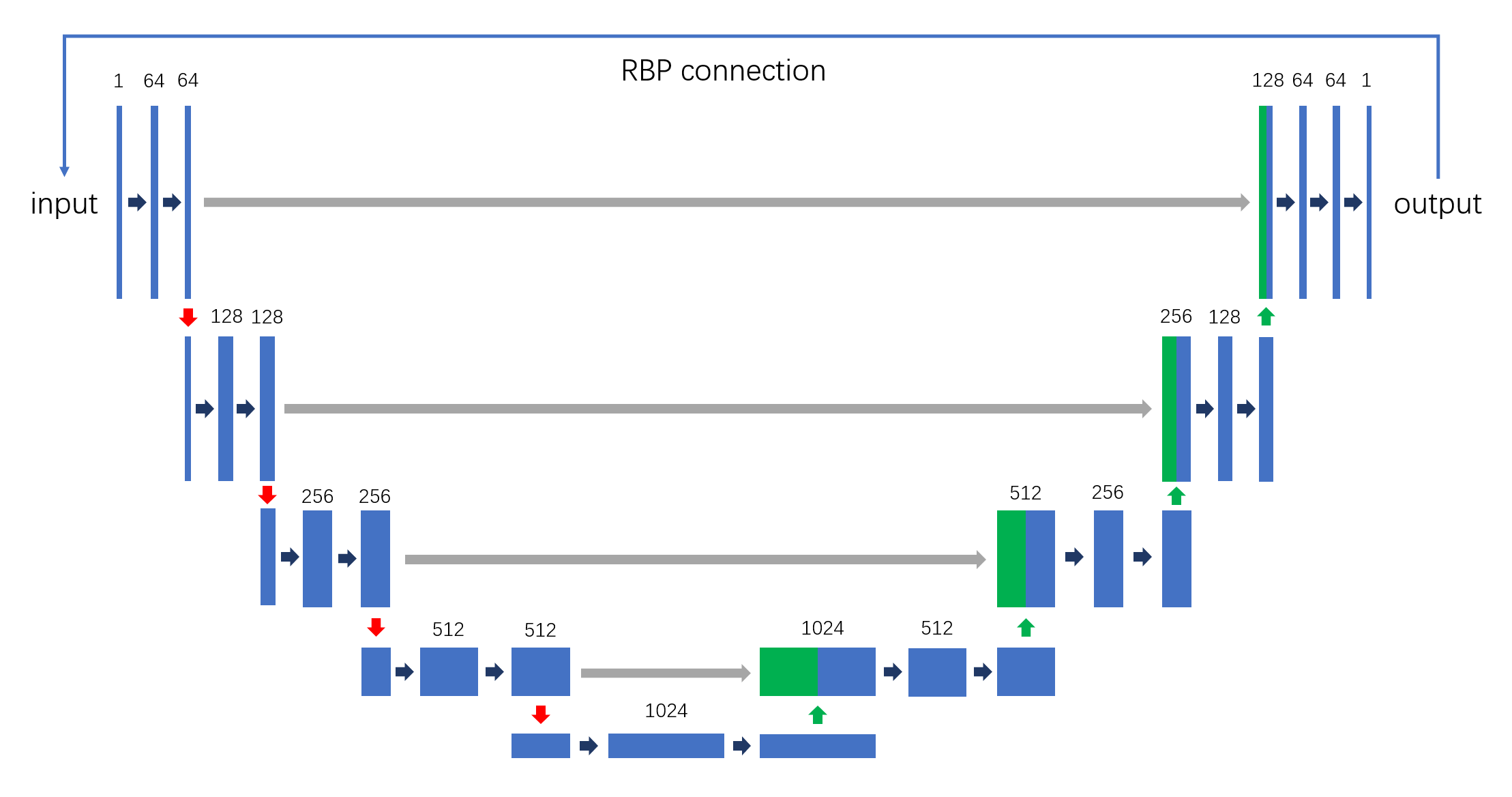
Fig. 1: The network architecture of the proposed framework.

3 Methods

3.1 CT Reconstruction with Deep Image Prior

As discussed before, conventional IR methods guarantee high-quality reconstruction by regularizing the solution of the inverse problem. The DIP [32] can be utilized to further improve its performance, especially when the inverse problem is highly ill-posed. This can be represented as:

$$\boldsymbol{w}^{*} =\operatorname*{arg\,min}_{\boldsymbol{w}}||\boldsymbol{g}-\boldsymbol{A}G(\boldsymbol{w};\boldsymbol{z})||^{2}_{2},$$ (3)

$$\boldsymbol{c}^{*} =G(\boldsymbol{w}^{*};\boldsymbol{z}),$$

where $G(\boldsymbol{w};\boldsymbol{z})$ represents an untrained convolutional neural network, it takes $\boldsymbol{z}$ as the input and is parameterized by the weights $\boldsymbol{w}$. Here $\boldsymbol{z}$ is a Gaussian vector that is randomly initialized and then fixed.

It is worth mentioning that although Equation 2 and Equation 3 share many similarities, inverse GAN and DIP are fundamentally distinct algorithms. In Equation 2, a well-trained neural network $G(\boldsymbol{z};\boldsymbol{w}^{*})$ is given. Therefore, inverse GAN aims to find the optimal results in the space spanned by the given model by optimizing its input vector $\boldsymbol{z}$. In contrast, the neural network $G(\boldsymbol{w};\boldsymbol{z})$ in Equation 3 is randomly initialized. It aims to solve the optimization problem by modifying the weights $\boldsymbol{w}$ of the network.

The key difference between the conventional IR method (Equation 1) and the DIP method (Equation 3) is that the DIP method uses the output of $G(\boldsymbol{w};\boldsymbol{z})$ to represent the reconstruction result $\boldsymbol{c}$. DIP related methods utilize the untrained neural network $G$ to minimize objective function by optimizing the network weights. In that case, the reconstruction result is constrained to lie in the range of images generated by that untrained neural network, so that the DIP property mostly ensures the generation of high-quality results, especially when the corresponding inverse problem is highly ill-posed. Furthermore, both DIP and IR methods minimize a similar loss function (regularizations can also be applied to Equation 3 [19]). This ensures that the results of DIP are not inferior to those of IR under similar loss conditions. This stands in contrast to pre-trained models, whose results are unpredictable. However, DIP related methods are susceptible to blurring and neural network specific artifacts. These shortcomings are demonstrated in Fig.7d, and Fig.8d. It is evident that the reconstruction results of the DIP method suffer from abnormal artifacts when the corresponding inverse problem is ill-posed (few-view and limited-angle CT reconstruction), and lack image details even when the problem is well-posed (full-view CT reconstruction).

3.2 Residual Back Projection with Deep Image Prior

Algorithm 1 RBP-DIP

Input: measure matrix $\boldsymbol{A}$, measurement $\boldsymbol{g}$, output $\boldsymbol{c}$ (zero at the beginning), input $\boldsymbol{z}$ (zero at the beginning), and step size $\beta$. The untrained model $G$ indicates the U-net in Fig.1 without the RBP connection.

1:$\boldsymbol{r}$ = $\boldsymbol{A}^{\rm T}\boldsymbol{g}-\boldsymbol{A}^{\rm T}\boldsymbol{A}\boldsymbol{c}$

2:$\boldsymbol{z}=\boldsymbol{z}+\frac{\boldsymbol{r}}{||\boldsymbol{r}||_{2}^{2}}$

3:$\boldsymbol{z}=\frac{\boldsymbol{z}}{||\boldsymbol{z}||_{2}^{2}}$

4:Repeat:

5: $\boldsymbol{c}=G(\boldsymbol{w};\boldsymbol{z})$

6: $\boldsymbol{r}$ = $\boldsymbol{A}^{\rm T}\boldsymbol{g}-\boldsymbol{A}^{\rm T}\boldsymbol{A}\boldsymbol{c}$

7: $\boldsymbol{z}=\boldsymbol{z}+\beta\frac{\boldsymbol{r}}{||\boldsymbol{r}||_{2}^{2}}$

8: $\boldsymbol{z}=\frac{\boldsymbol{z}}{||\boldsymbol{z}||_{2}^{2}}$

9: update $\boldsymbol{w}$ by using $||\boldsymbol{r}||_{2}^{2}$

10:Until: convergence, or some fixed number of iterations is reached.

11:Optional: apply IR algorithm on $\boldsymbol{c}$.

The architecture of our proposed framework, residual back projection with the deep image prior (RBP-DIP), is shown in Fig.1. It contains a U-net and an RBP connection. The U-net, which has demonstrated its efficacy in various image processing problems, is used to implement the standard DIP algorithm in our approach. In each iteration, the input of the U-net is iteratively updated using the residual between the sinogram of the current network output and the provided measurement via the RBP connection. This update incorporates the information from the conventional IR algorithm and can be used to enhance the output of the U-net. The RBP connection constitutes the primary distinction between our RBP-DIP model and the DIP model presented in [32, 26]. Notably, the RBP connection does not participate in the backpropagation process.

An intuitive explanation of RBP-DIP is that it uses a conventional IR method to update the input of the neural network, and uses the output of the neural network as the input of the conventional IR method. Such an architecture is designed to take advantage of both the conventional IR method and the DIP method.

The DIP property can help the untrained U-net generate high-quality images that are free from most artifacts existing in conventional IR methods, especially when the corresponding inverse problem is highly ill-posed. However, this method is always considered unstable and may generate neural network specific artifacts, as the whole neural network is randomly initialized and cannot be clearly explained. On the contrary, although the conventional IR methods are unable to generate accurate reconstruction results when the inverse problem is highly ill-posed, its convergence rate, stability, and robustness have already been well-analyzed. Thus, it can be used to guide the DIP method, correct the aforementioned network specific artifacts, fine-tune the reconstruction result, and increase the robustness of the whole framework. As a result, the integration of the RBP connection and DIP method can amalgamate the advantages of both methods and mitigate each other’s shortcomings.

The details of RBP-DIP are shown in Algorithm 1, where lines 1-3 and 6-8 correspond to the RBP connection. Lines 5, 6, and 9 correspond to the optimization of the untrained U-net. In the proposed framework, the output vector $\boldsymbol{c}$ is employed to update the input for the subsequent iteration through the RBP connection. It is postulated that the iteratively corrected vector $\boldsymbol{z}$ can more effectively guide the model since the correction primarily targets edge features and neural network-specific artifacts. In this paper, the RBP connection only back projects the sinogram residual for the sake of simplicity. However, it is evident that a more delicate IR update technique can also be utilized to further enhance its overall efficacy.

It is worth mentioning that substantial fluctuations in the input to the U-net could undermine its stability and overall performance. Consequently, we normalize the input $\boldsymbol{z}$ in lines 3 and 8 so that the input of the U-net is always a unit vector. Moreover, the magnitude of RBP updates necessitates regulation, as the RBP updates would otherwise dominate the reconstruction process and lead to artifacts commonly seen in conventional IR methods. In that case, the residual $\boldsymbol{r}$ is also normalized in lines 2 and 7. Together with the function $\beta$, the RBP update in line 7 is a summation of the previous unit vector $z$ and another vector of length $\beta$, which can be expressed as:

$$\beta=\frac{10^{-3}}{1+e^{-(\frac{n}{n_{s}}-n_{c})}},$$ (4)

where $n$ indicates the current number of iterations. $\beta$ is a sigmoid function centered at $n_{c}$ and stretched by the factor $n_{s}$. In the initial phase of the reconstruction procedure ($\frac{n}{n_{s}}\ll n_{c}$), the DIP property plays a crucial role in generating high-quality preliminary reconstruction outcomes. During this period, the RBP connection is suppressed by the factor $\beta$ to avoid introducing artifacts commonly associated with IR methods. As the reconstruction progresses and $\frac{n}{n_{s}}\gg n_{c}$, the RBP connection’s strength is augmented by the increasing $\beta$. In this later stage, the RBP connection serves to further refine the reconstruction without engendering additional artifacts, given that a high-quality preliminary reconstruction has already been generated. To achieve optimal performance, it is imperative for $n_{c}$ to be sufficiently large to yield a smooth function, preventing significant disruptions to the network stability caused by input updates. The selection of $n_{c}$ mainly depends on the nature of the inverse problem itself. In instances where the inverse problem is highly ill-posed, characterized by conditions such as few-view and limited-angle scenarios, conventional iterative reconstruction (IR) methods implemented in the proposed RBP connection may result in pronounced artifacts. In such cases, it is advisable to use a larger $n_{c}$. This adjustment gives the algorithm more time to leverage the properties of deep image priors (DIP) for obtaining a better initial guess. Conversely, if the inverse problem is closer to being well-posed or over-determined, a smaller $n_{c}$ enables the RBP to take in the optimization process more promptly. In our experiments, for simplicity, we have set the parameters to $n_{s}=500$, $n_{c}=10$, and the total number of iterations is $10000$. By employing these values, the RBP connection is suppressed during the first half of the reconstruction process and gradually augmented during the second half.

Since the core of the RBP-DIP algorithm is an untrained neural network, its convergence properties cannot be strictly proven. To mitigate potential adverse effects, we propose a conventional IR algorithm at line 11 as a post-processing step. This aims to ensure convergence and eliminate potential artifacts generated by the neural network. The procedure is optional, as numerous studies [29, 32, 4, 26, 21, 12] indicate that the algorithm converges and yields favorable outcomes with high possibility. In all subsequent experiments presented in this paper, we omit the post-processing step and still observed excellent results.

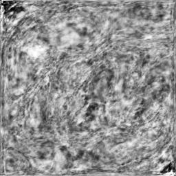
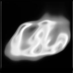
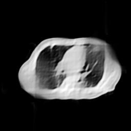
(a) 1st Iteration

(b) 10th Iteration

(c) 20th Iteration

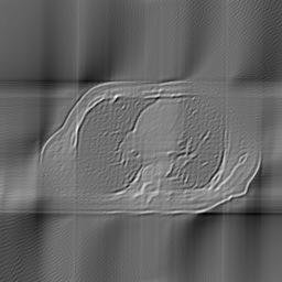
(d) 2000th Iteration

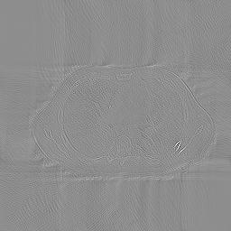
(e) 10000th Iteration

Fig. 2: The output (first row) and the corresponding input $\boldsymbol{z}$ (second row) at different iteration. The number of views is $90$, uniformly distributed from $0^{\circ}$ to $90^{\circ}$.

(a) Ground Truth

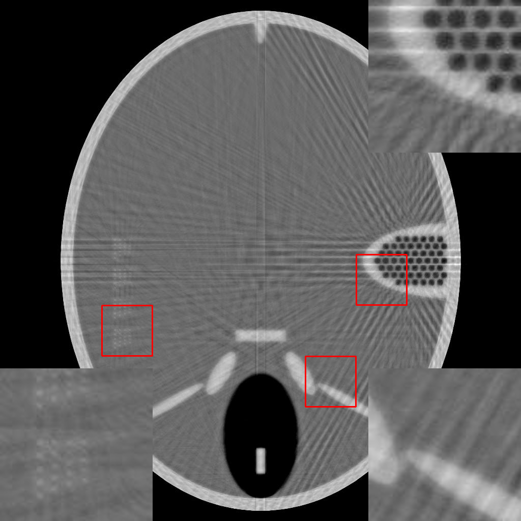
(b) 19.01dB

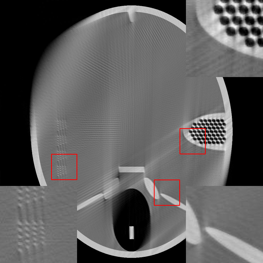
(e) 15.35dB

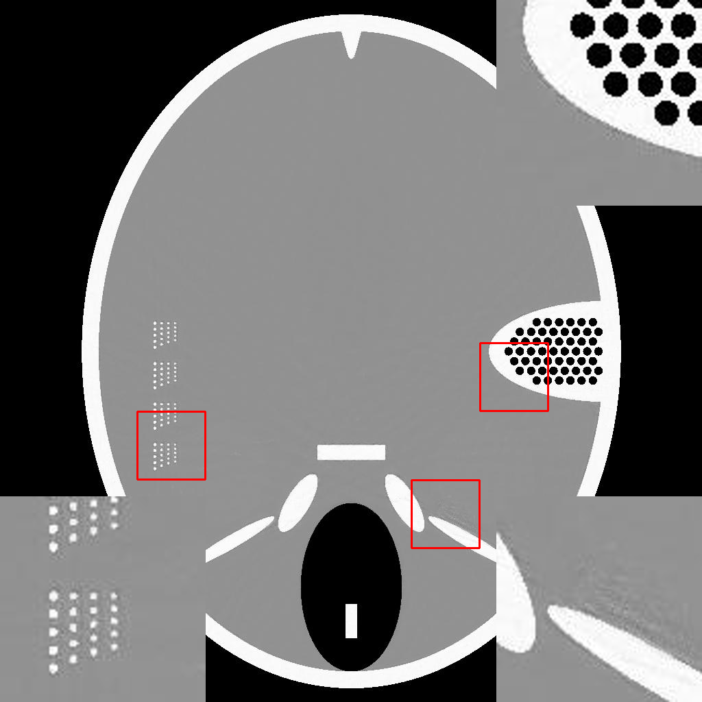
(c) 37.72dB

(f) 20.54dB

(d) 38.96dB

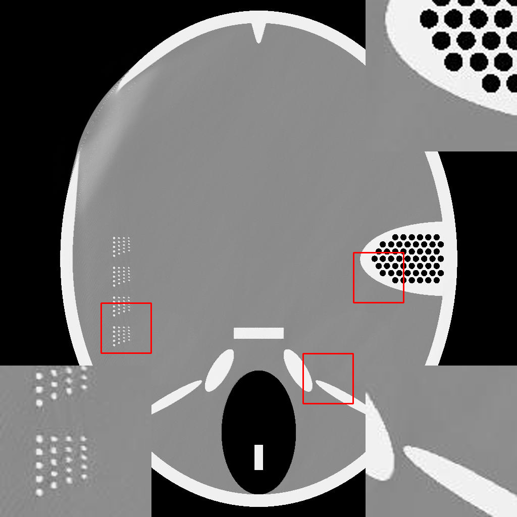
(g) 22.84dB

Fig. 3: The few-view (first row) and limited-angle (second row) reconstruction results of the Forbild phantom for ASD-POCS (second column), DIP (third column), and RBP-DIP (last column).

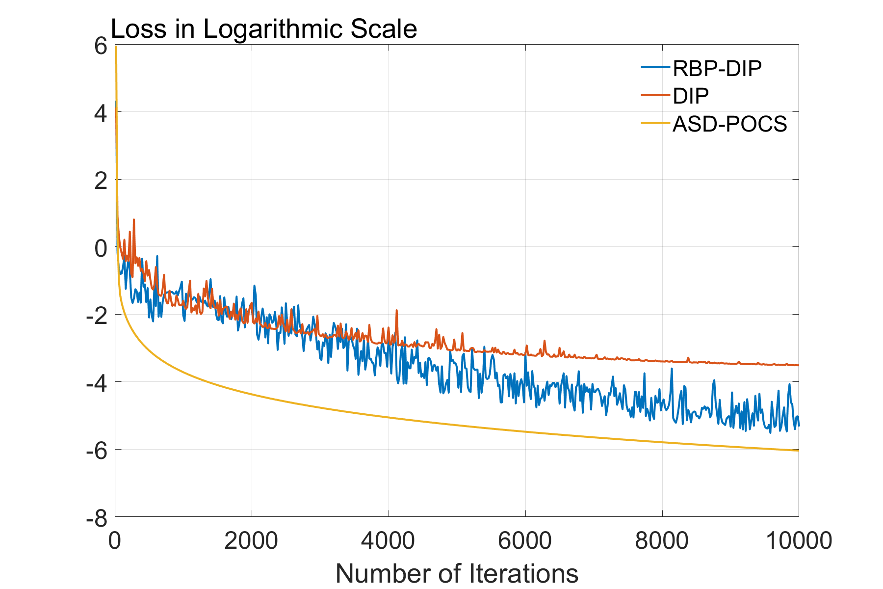
(a)

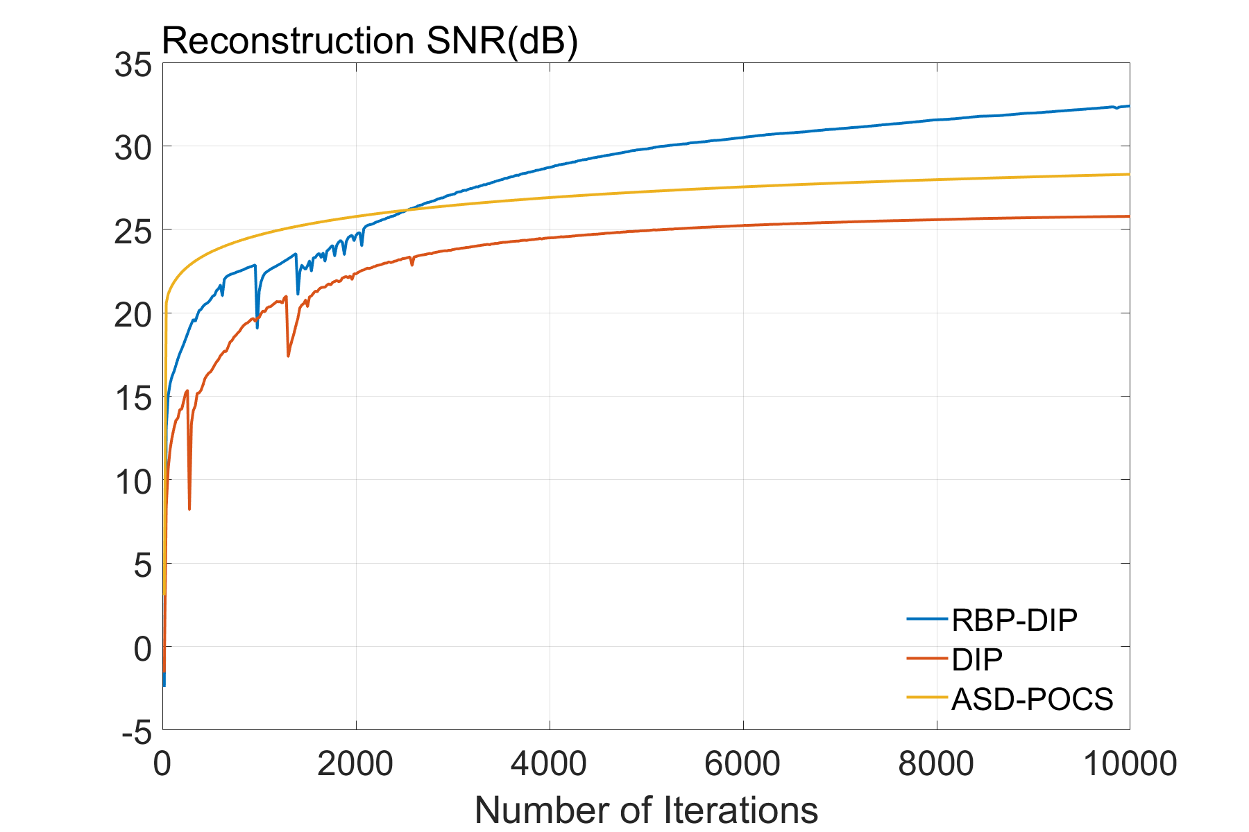
(b)

Fig. 4: The reconstruction loss ($l_{2}$ norm in logarithmic scale) and SNR (dB) of different methods under few-view condition (number of views is $90$, uniformly distributed from $0^{\circ}$ to $180^{\circ}$). RBP-DIP achieves higher SNR with a loss larger than ASD-POCS method.

4 Experiments and Results

In this section, we first conduct experiments showing the effect of the RBP connection. We also compare the differences between the proposed framework and the well-established IR algorithm ASD-POCS (adaptive steepest descent projection onto the convex set) [28] under multiple conditions. In that case, the effect of employing an untrained neural network for iterative reconstruction can be assessed. In addition, the proposed method is also compared with the state-of-the-art DIP model [4] as well as two widely recognized pre-trained models MED50 [15] and RED-CNN [8]. The structural similarities among these models show the merits of the proposed method while eliminating model complexity bias. The aforementioned methods are first tested under parallel-beam geometry. The Gram filtering method proposed by Shu and Entezari [25] is used to calculate the forward and back projection exactly and efficiently. Next, $512\times 512$ reconstructions under fan-beam geometry are conducted, where the ASTRA toolbox’s [30] line_fanflat projector is used for forward and back projection. To address potential issues related to inverse crime, sinogram data $\boldsymbol{g}$ is acquired from upsampled ($1024\times 1024$) ground truth images.

The aforementioned neural networks are implemented in Python with the PyTorch library. The RMSProp algorithm serves as the optimizer, with a learning rate set to $1\times 10^{-4}$, which decreases by a factor of $0.9$ every $500$ iterations. The hyperparameters utilized in the RBP-DIP framework are assigned the values $n_{s}=500$, and $n_{c}=10$. Images from LIDC-IDRI [3] (The Lung Image Database Consortium image collection) dataset are used in our experiments.

It is worth mentioning that each pre-trained model is retrained for different settings such as the number of views, and projection angular range. Moreover, during the training procedure, test images are employed for the direct assessment of the pre-trained models, while validation images are not utilized in this context. Although impractical in the real world, this ensures the attainment of optimal reconstruction outcomes for the test images.

4.1 Effect of Residual Back Projection in Reconstruction

In order to demonstrate the efficacy of the RBP connection and show the details of the RBP-DIP’s reconstruction process, the procedure of a limited-angle CT reconstruction is shown in Fig.2. Its first row shows the reconstruction outcomes of varying iterations, while the second row shows the corresponding input of the U-net, which has been updated through the RBP connection. Here, the number of views is set to $90$, uniformly distributed from $0^{\circ}$ to $90^{\circ}$. This scenario presents a challenging limited-angle CT reconstruction problem.

In the first iteration, as depicted in Fig.2a, the input image undergoes an update via the RBP connection prior to being fed to the U-net. Thus, this input is the normalized first iteration output of the implemented IR algorithm (normalized back projection image in our case). The output appears completely randomized since the entire neural network is randomly initialized.

In the 10th and 20th iterations (Fig.2b and Fig.2c), the DIP property effectively expedites the recovery of the object over its support. Of note are lack of artifacts commonly caused by having missing views in the data. The input images highlight the region which can be relatively accurately reconstructed by conventional IR methods. This can be used to guide the model in the later iteration. In our experiment, the model capitalizes on the input images more when reconstructing the top left and the bottom right parts of the image, while relying predominantly on the DIP property for the reconstruction of the top right and the bottom left parts.

In the 2000th iteration, as depicted in Fig.2d, the reconstruction result becomes relatively artifact-free. At this stage, the input image of the U-net primarily emphasizes the edges to help the method improve the supporting area. Moreover, the RBP connection can rectify artifacts specific to convolutional neural networks. Evidence of this can be observed in the second row of Fig.2c, Fig.2d, and Fig.2e, which display distinct horizontal and vertical patterns. These patterns are mainly caused by the convolution operation in the U-net. In other words, the DIP and RBP parts of the proposed framework are able to mutually rectify each other’s errors. Consequently, a high-quality reconstruction result is attainable, as shown in Fig.2e.

4.2 Effect of Residual Back Projection with Deep Image Prior

A direct comparison among the proposed RBP-DIP, the widely used IR method ASD-POCS, and the current untrained method [4] is made to show the advantages of the proposed framework. Given that the number of views is set to $90$, uniformly distributed from $0^{\circ}$ to $180^{\circ}$, the scenario presents a challenging few-view CT reconstruction problem. The reconstruction performance in terms of reconstruction loss and SNR is shown in Fig.4. From Fig.4a, it is evident that comparing to DIP, RBP-DIP can better minimize the objective function. Although the ASD-POCS method can further minimize the objective function, Fig.4b shows that RBP-DIP achieves the highest SNR. This indicates that when the problem is highly ill-posed, where multiple solutions can minimize the objective function, the result chosen by RBP-DIP is better than others. Another thing worth mentioning is that the loss of RBP-DIP shown in Fig.4a is fluctuating, which is in line with our analysis in Section 3.2. This implies that using the conventional IR method to fine-tune the output RBP-DIP can further improve its reconstruction results.

For a more direct comparison, the three aforementioned methods are tested on the Forbild phantom under few-view ($60$ views, uniformly distributed from $0^{\circ}$ to $360^{\circ}$), and limited-angle ($120$ views, uniformly distributed from $0^{\circ}$ to $120^{\circ}$). From Fig.3, it is clear that both the DIP and RBP-DIP exhibit superior performance compared to ASD-POCS, particularly in the reconstruction of detailed structures. The magnified views of these structures are available in the bottom left and top right corners of these images. In contrast to DIP, RBP-DIP is better at mitigating some neural network-specific artifacts, with the corresponding magnified view presented in the bottom right corner of these images.

It is worth mentioning that another significant factor contributing to the substantial advantage of DIP and RBP-DIP over ASD-POCS is the piece-wise constant nature of the Forbild phantom. Therefore, to better assess the performance of the proposed method in practical applications, multiple experiments using real CT images are conducted in the following sections.

4.3 Few-View CT Reconstruction

In this section, the reconstruction performance of our proposed framework under few-view conditions will be tested. For the parallel-beam and fan-beam geometry, the number of views increases from $30$ to $180$, uniformly distributing from $0^{\circ}$ to $180^{\circ}$ and $0^{\circ}$ to $360^{\circ}$ respectively. Such settings provide a complete benchmark of reconstruction performance, ranging from extremely sparse to relatively complete, full-view CT reconstruction. The experiment results are shown in Fig.5. Additionally, the ground truth, few-view ($30$ views), and full-view ($180$ views) CT reconstruction results of different methods are shown in the first and third rows of Fig.7 (parallel-beam, LIDC-IDRI dataset), and Fig.8 (fan-beam, LIDC-IDRI dataset).

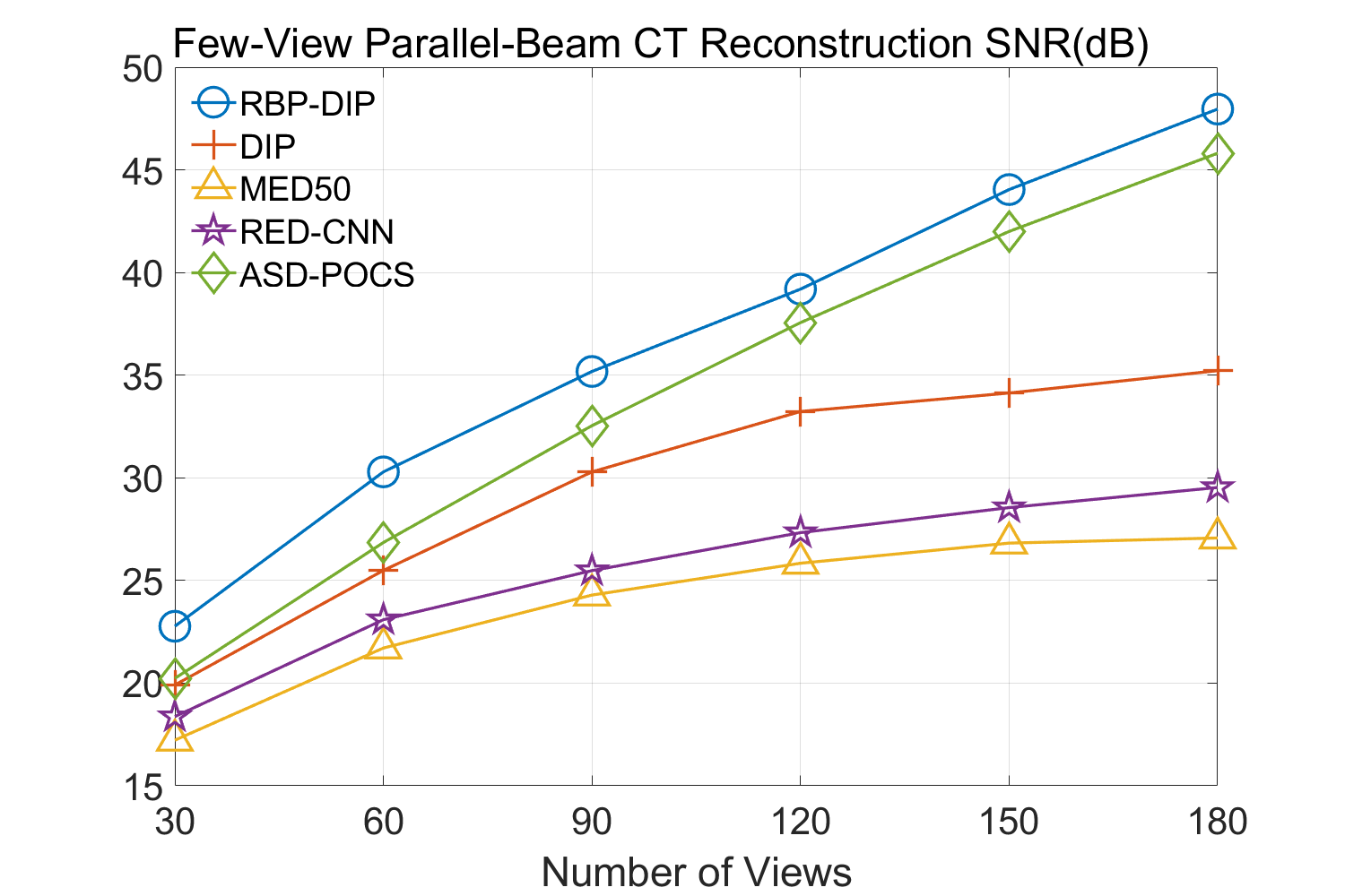
(a)

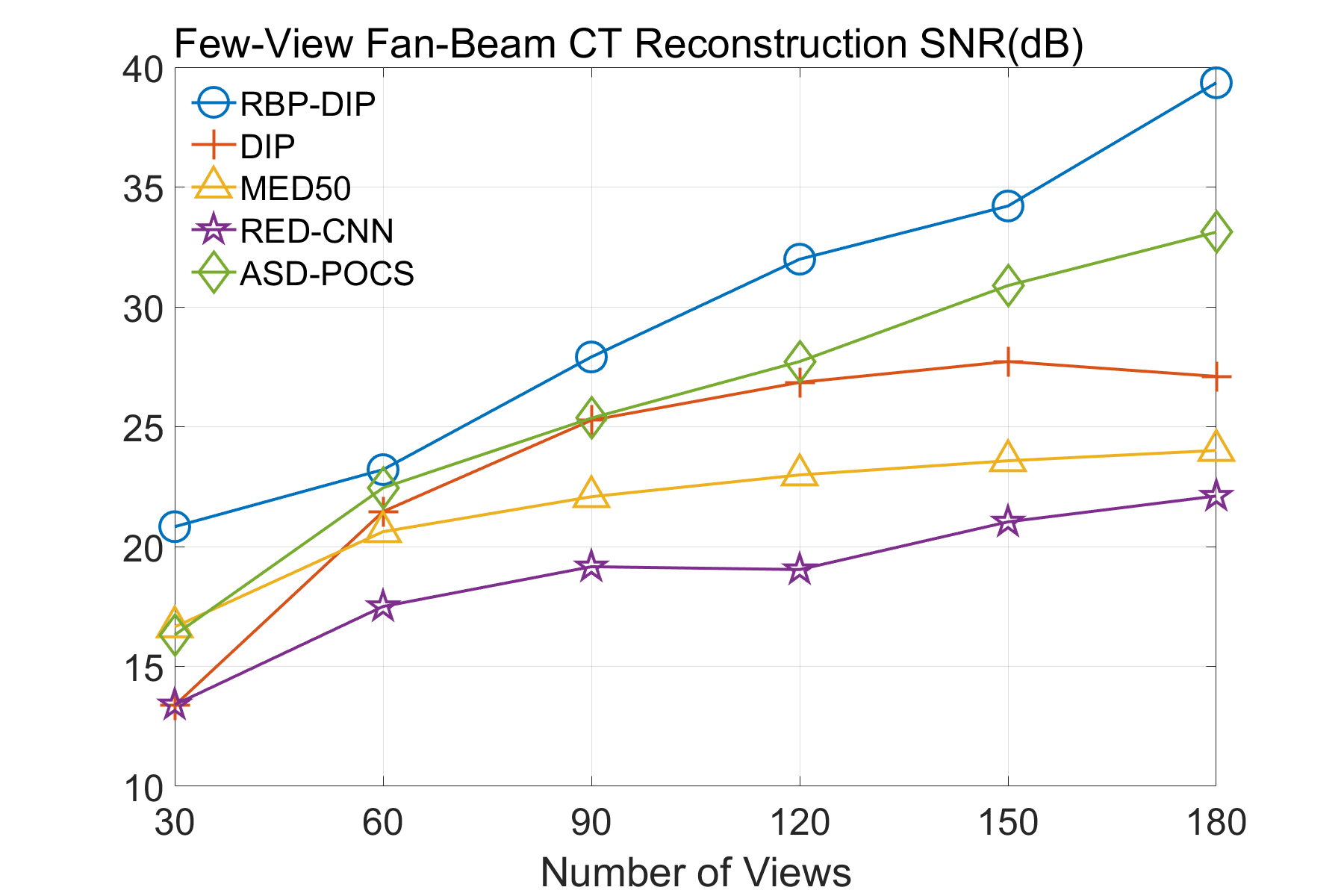
(b)

Fig. 5: The performance of few-view CT reconstruction for different methods under different numbers of views and geometries.

4.4 Limited-Angle CT Reconstruction

To test the proposed framework’s performance on limited-angle reconstruction, we redo the experiment in the above section with the angular range changing from $0^{\circ}-90^{\circ}$ to $0^{\circ}-165^{\circ}$ for parallel-beam geometry and $0^{\circ}-90^{\circ}$ to $0^{\circ}-180^{\circ}$ for fan-beam geometry, one projection per degree. The experiment results are shown in Fig.6. Also, the ground truth and the limited-angle CT reconstruction results of different methods are shown in the row of Fig.7 (parallel-beam, LIDC-IDRI dataset), and Fig.8 (fan-beam, LIDC-IDRI dataset).

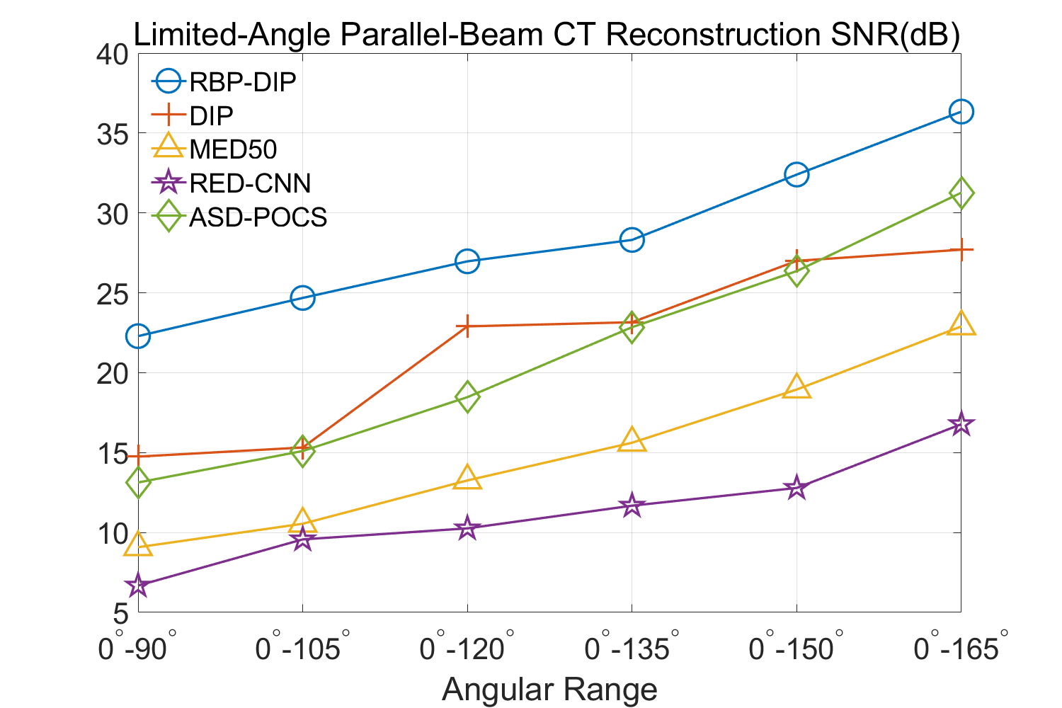
(a)

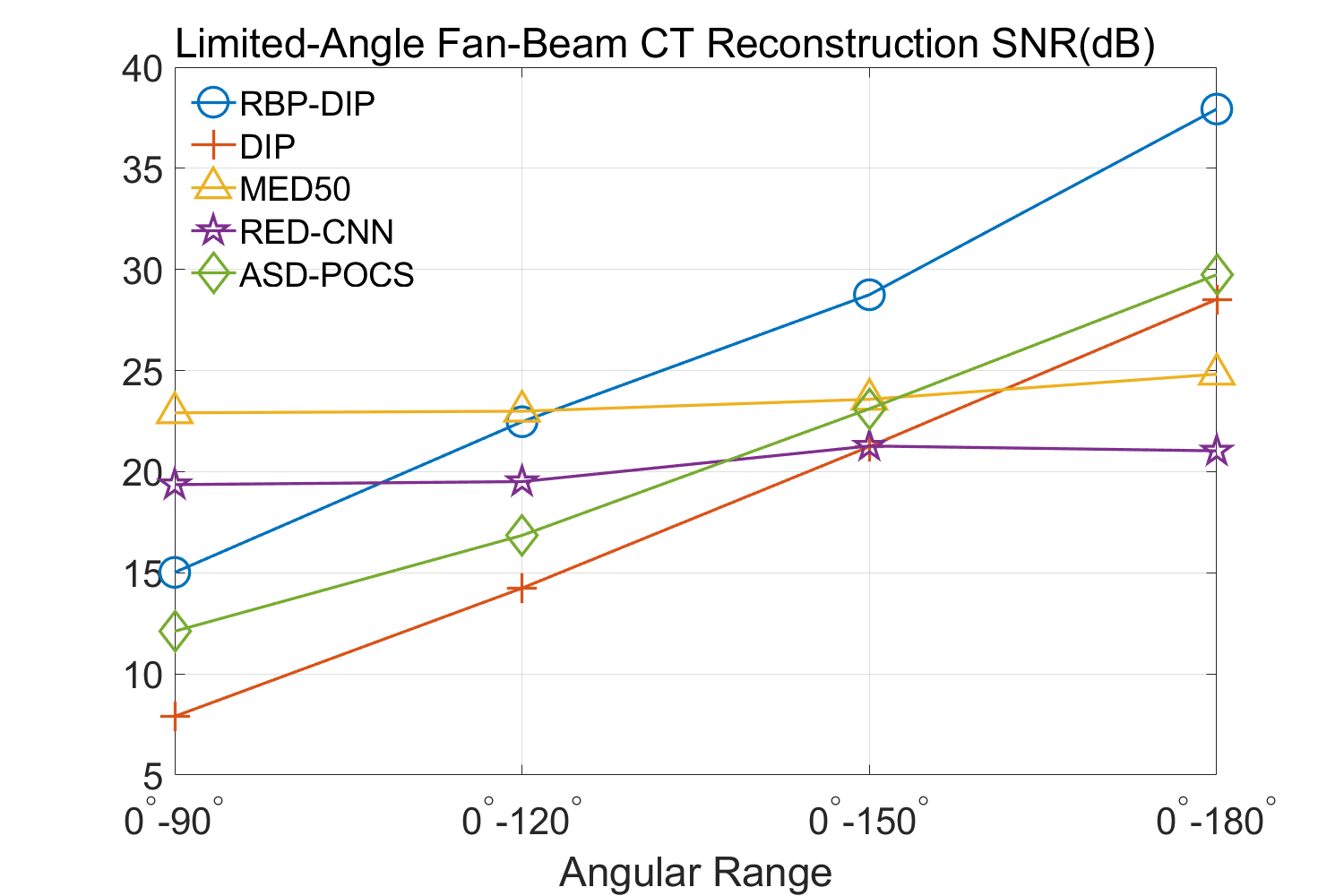
(b)

Fig. 6: The performance of limited-angle CT reconstruction for different methods under different angular ranges and geometries.

20.23dB

24.92dB

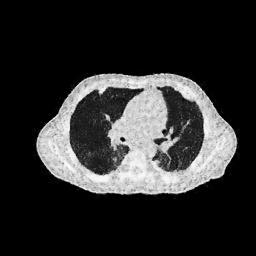
19.9dB

17.22dB

17.88dB

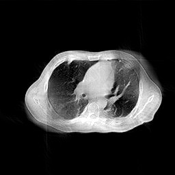
12.69dB

22.87dB

11.75dB

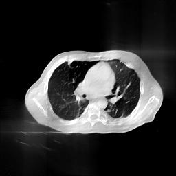
9.08dB

6.18dB

(a) Ground Truth

43.87dB

(b) ASD-POCS

47.96dB

(c) RBP-DIP

34.46dB

(d) DIP

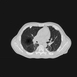
26.63dB

(e) MED50

29.03dB

(f) RED-CNN

Fig. 7: The parallel-beam reconstruction results of LIDC-IDRI dataset for different methods under few-view (first row, 30 projections distributed uniformly from $0^{\circ}$ to $180^{\circ}$), limited-angle (second row, 90 projections distributed uniformly from $0^{\circ}$ to $90^{\circ}$) and full-view (third row, 180 projections distributed uniformly from $0^{\circ}$ to $180^{\circ}$) conditions.

16.31dB

20.83dB

13.37dB

16.65dB

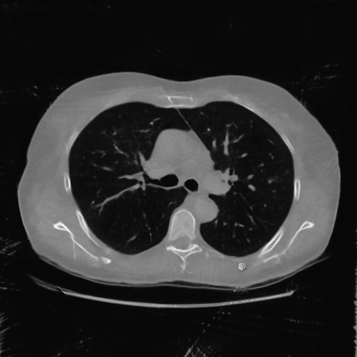
13.40dB

16.85dB

22.47dB

14.25dB

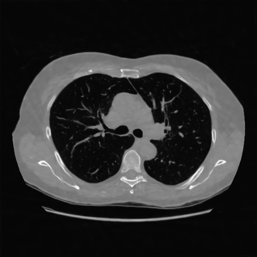
22.99dB

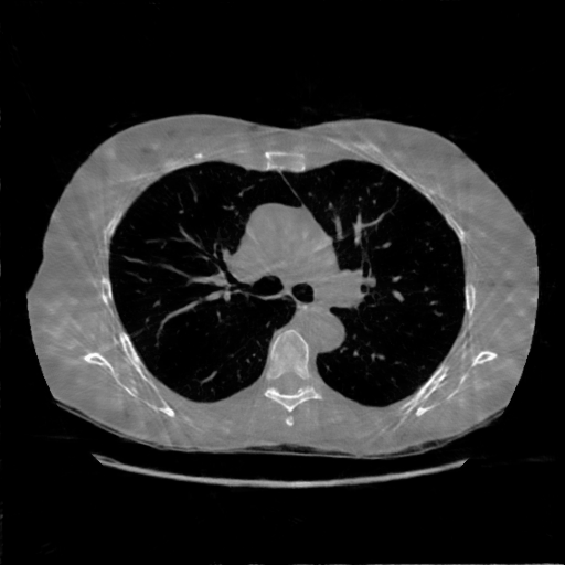
19.51dB

(a) Ground Truth

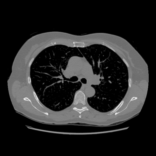
30.15dB

(b) ASD-POCS

39.35dB

(c) RBP-DIP

27.10dB

(d) DIP

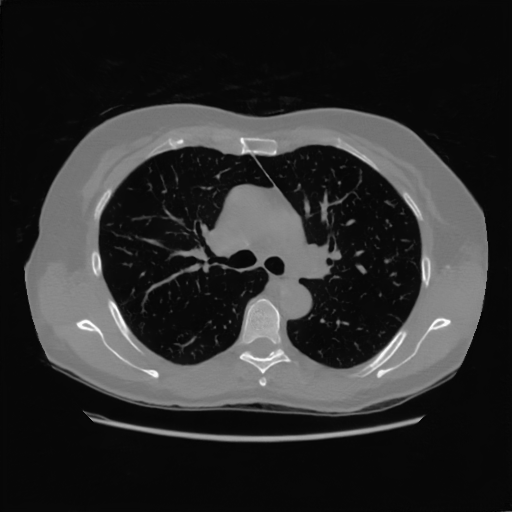
23.88dB

(e) MED50

20.59dB

(f) RED-CNN

Fig. 8: The fan-beam reconstruction results of LIDC-IDRI dataset for different methods under few-view (first row, 30 projections distributed uniformly from $0^{\circ}$ to $360^{\circ}$), limited-angle (second row, 120 projections distributed uniformly from $0^{\circ}$ to $120^{\circ}$) and dense-view (third row, 180 projections distributed uniformly from $0^{\circ}$ to $360^{\circ}$) conditions.

4.5 Non-Ideal Factors

As previously mentioned, one of the most significant advantages of our proposed method lies in the elimination of the training process. This advantage precludes any potential hindrances arising from an insufficient training procedure or inconsistencies between inference input and training dataset. To examine this assertion, experiments under multiple non-ideal conditions have been conducted.

4.5.1 Rotation

The few-view CT reconstruction experiment is replicated, utilizing an identical test image rotated by $30^{\circ}$ degrees to simulate a rudimentary pose alteration of the patient. The reconstruction performances are shown in Fig.9, and the reconstruction results corresponding to $30$ views are shown in Fig.10. A similar experiment is also conducted under the limited-angle condition, yielding similar results.

4.5.2 Quantum Noise

To test the proposed method’s performance under the low-dose condition, we repeat the aforementioned reconstruction experiments by using the sinogram data polluted with Poisson-distributed noise. The average number of X-ray photons received by the $i$th detector can be expressed as:

$$E_{i}=I_{0}e^{-g_{i}},$$

where $I_{0}>0$ is the blank measurement ($g_{i}=0$). It is worth mentioning that the sinogram measurements employed in this study are derived from simulations, as opposed to being sourced from an actual instrument. Thus, $I_{0}$ here is a parameter for relative measurement. Throughout the experiments, $I_{0}$ is assigned values ranging from $10^{2}$ to $10^{8}$, which correspond to sinogram SNR (dB) values of $25.6,35.6,...,85.6$. It is worth mentioning that analogous experiments were conducted under both few-view and limited-angle scenarios, with the proposed method demonstrating a marked superiority over other methods across all conditions. This enhancement, however, is primarily attributed to the exceptional performance of the proposed method under sparse-measurement circumstances, rather than an increased resistance to noise. To facilitate an equitable comparison, the results displayed in Fig.11 are solely derived from the full-view scenario, which encompasses an angular range of $0^{\circ}-180^{\circ}$ with one view per degree.

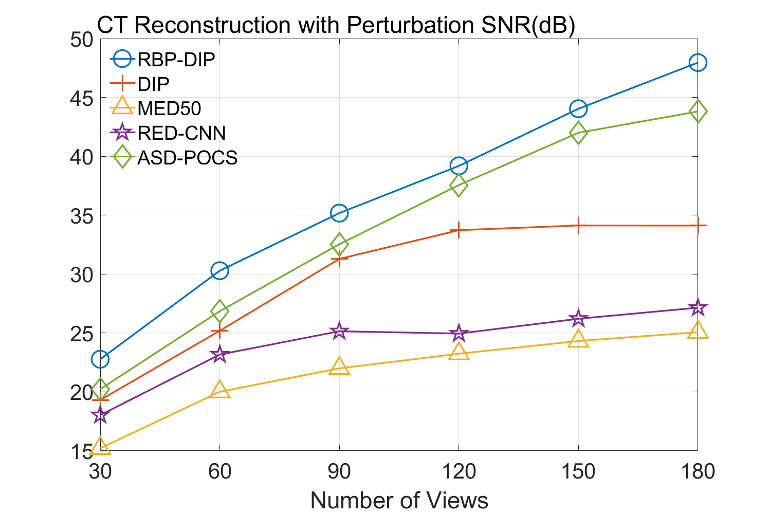
Fig. 9: The performance of few-view CT reconstruction with perturbation (rotated by $30^{\circ}$) for different methods.

(a) ASD-POCS (19.92dB)

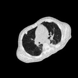
(b) RBP-DIP (23.82dB)

(c) DIP (21.88dB)

(d) MED50 (15.61dB)

Fig. 10: The few-view ($30$ views) CT reconstruction results with perturbation (rotate by $30^{\circ}$) of different methods.

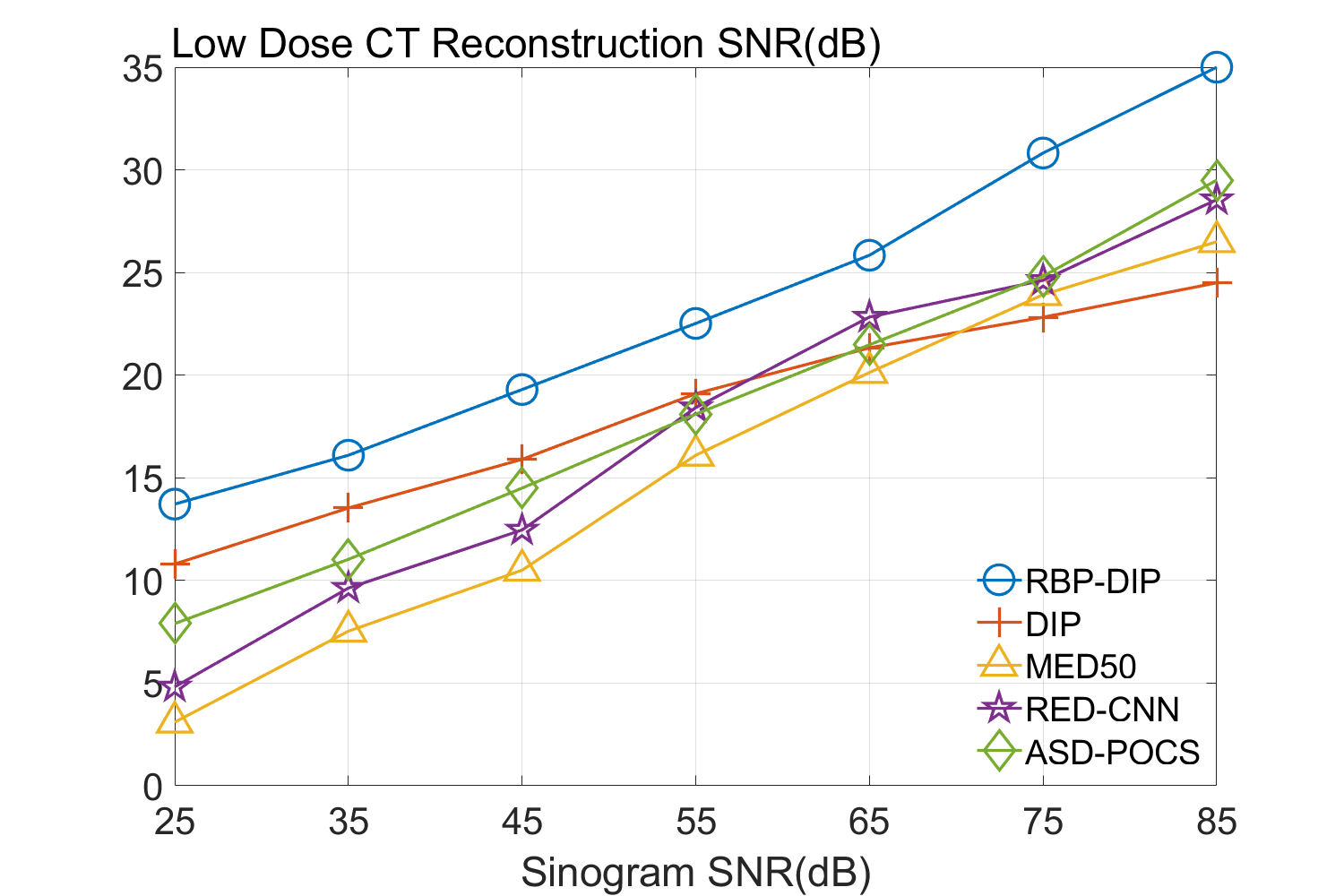
Fig. 11: Effect of quantum noise modeled by Poisson distribution in the sinogram on reconstruction SNR(dB).

5 Discussion

5.1 Comparisons on DIP, IR, and RBP-DIP

It is worth mentioning that both DIP and RBP-DIP are iterative reconstruction methods since all these methods reconstruct images by minimizing an objective function iteratively. This minimization process offers a dependable lower bound, ensuring that their performance does not fall below that of conventional IR methods. The distinction between conventional IR and DIP related methods lies in the use of an untrained convolutional neural network.

Conventional IR methods, even those with the help of regularizations such as total variation, are prone to artifacts when constrained by few-view and limited-angle conditions. However, as illustrated in the first and second rows of Fig.7b, and Fig.8b, these images still contain meaningful information which can be used to guide DIP related reconstruction methods, despite the presence of artifacts.

DIP related methods, which leverage the hierarchical structure of neural networks as a powerful prior, can better handle the aforementioned challenge. However, the original DIP method has its own limitations. It cannot generate detailed images or effectively enhance its accuracy as the number of measurements increases. For instance, in Fig.5a, the ASD-POCS algorithm achieves an approximate SNR gain of $25$dB when the number of views increases from $30$ to $180$, while the DIP method only attains an approximate $15$dB gain. This problem is also shown in the last row of Fig.7, and Fig.8. Moreover, the DIP method may produce neural network specific artifacts, as shown in Fig.7d, and Fig.8d. These artifacts are particularly problematic as they are often considered more undesirable than streak artifacts. Radiologists, with their professional experience, can interpret and account for streak artifacts, whereas network specific artifacts may prove more challenging to identify and address.

The proposed RBP-DIP framework combines the two approaches utilizing the newly devised RBP connection so that inherits the benefits of both methods. In Fig.4, the RBP-DIP method’s attainment of a 5dB SNR enhancement over the ASD-POCS method, despite exhibiting a larger loss, underscores the potency of the DIP. Subsequently, the improvement surpassing the original DIP method indicates the efficacy of the RBP connection. Moreover, by employing the RBP connection, neural network specific artifacts can be rectified effectively. As a result, substantial advancements can be shown in Fig.5, Fig.6, Fig.7, and Fig.8.

5.2 Comparing with Pre-Trained Models

We have also conducted comparative analyses with pre-trained models MED50 and RED-CNN under multiple conditions. These models share similar network structures and complexities with the RBP-DIP framework. We have opted not to examine models with more complicated networks, as the proposed method is untrained, necessitating a focus on the structural properties of the networks for equitable comparisons. Theoretically, pre-trained models should outperform the proposed framework in most cases, especially when the number of measurements is not enough, as they can acquire extra information from training datasets. However, as shown in Fig.5 and Fig.6, RBP-DIP outperforms the two pre-trained models in most cases, with the only exception being limited-angle fan-beam reconstruction where the angular range is $0^{\circ}-90^{\circ}$.

Pre-trained models’ low performances may be caused by the limited number of views. In the original research, the network inputs are high-quality FBP images (with 400 views), which possess sufficient projections and relatively minimal artifacts. In that case, the inconsistencies between the input and the corresponding output are relatively small, so that pre-trained models can learn the correct prior with limited training data. In our experiments, the FBP images always suffer from severe artifacts, and the aforementioned differences are relatively large. As a result, pre-trained models cannot be trained properly without a large, high-quality training dataset. In fact, some training instances in the current training dataset may even downgrade the performance of pre-trained models due to discrepancies in postures and CT slices, as illustrated in Fig.12.

Also, Fig.5 and Fig.6, particularly Fig.6b, show that an increasing number of views does not sufficiently lead to improved performance of pre-trained models. The reason is that pre-trained models aim to learn the mapping between the input and the corresponding output from training datasets, rather than actually solve the corresponding inverse problem. Increasing the number of views cannot directly strengthen this mapping. Conversely, the proposed RBP-DIP directly minimizes the inconsistency between the ground truth and reconstructed images under the same measurements. Increasing the number of views reduces the dimensions of the solution space and thus benefits both network optimization and the iterative reconstruction (IR) algorithms integrated in the RBP connection. This outcome is further verified in the last row of Fig.7, and Fig.8, where RBP-DIP considerably outperforms other methods.

Fig. 12: Training instances in LIDC-IDRI dataset. Some of the training instances may even downgrade the performance of pre-trained models, as they are different from the inference images due to the inconsistency in postures and CT slices.

5.3 Non-Ideal Factors

In practical applications, the imaged object might exhibit inconsistencies with the training dataset due to various non-ideal factors. The $30^{\circ}$ rotation operation in Section 4.5 serves as a simplified simulation of such discrepancies, which may arise from differing poses of patients. The impact on reconstruction accuracy is shown in Fig.9. The comparison between Fig.5b and Fig.9 reveals that the pre-trained MED50 method is predominantly affected by a considerable decline in SNR. The reconstruction results are also presented in Fig.10. In contrast to the first row of Fig.7, the MED50 reconstruction result lacks a completely black background and exhibits horizontal artifacts in the non-empty region. This observation suggests that MED50 cannot effectively handle the perturbations in the inference data.

Additionally, experiments were conducted under low-dose conditions, as demonstrated in Fig.11. MED50 was found to be the most vulnerable to sinogram noise, while RED-CNN exhibited relative insensitivity to perturbations due to its patch-based learning approach.

The proposed RBP-DIP framework does not necessitate any training images and attains the highest reconstruction accuracy in both experiments. Moreover, additional constraints or regularizations can be directly incorporated into the objective function or indirectly integrated into the RBP connection, enabling enhanced handling of various factors without retraining.

5.4 Future Works and Prospects

This study shows that the RBP-DIP framework shows improvements over other methods in the CT reconstruction problem for both parallel-beam and fan-beam geometries under multiple conditions. Also, the RBP-DIP framework has great potential for further improvement. The RBP connection in this paper is implemented by the steepest descent algorithm without additional constraints or regularizations. However, it is evident that RBP-DIP is compatible with all other IR methods, constraints, and regularizations. Notably, these techniques can be incorporated into both the objective function and the RBP connection. In contrast to pre-trained models, these adjustments can be adapted on demand (e.g., augmenting the total variation regularization’s weight when dealing with noisy input data). Moreover, the proposed framework employs a basic U-net structure, but more sophisticated models such as U-net++[45] and ResUnet[44] might be integrated for further improvement.

Like DIP, the primary challenge faced by the RBP-DIP algorithm is its long computing time. Unlike the inference process of pre-trained neural networks, where the network is initialized with learned weights, the RBP-DIP network starts from a random initialization. The process of minimizing the loss function is equivalent to training a neural network from scratch with a training set of size $1$. In that case, in our upcoming research, we will focus on accelerating the RBP-DIP algorithm without compromising its accuracy.

6 Conclusion

In this paper, we present an untrained neural network related framework, RBP-DIP, for X-ray CT reconstruction. Remarkable reconstruction results are achieved using RBP-DIP without any training process or extra regularization, particularly under few-view, limited-angle, and low-dose conditions. The improvements are primarily attributable to the employment of the untrained neural network and the RBP connection, which utilize the advantages of DIP and conventional IR algorithms, respectively.

In comparison with conventional IR methods, RBP-DIP attains a higher signal-to-noise ratio (SNR), especially when the corresponding inverse problem is highly ill-posed. In comparison with the original DIP method, RBP-DIP exhibits superior accuracy and is free from neural network specific artifacts. These findings suggest that our proposed methodology successfully utilizes the advantages of both IR and DIP methods.

Comprehensive comparisons are also conducted with pre-trained models possessing similar network structures to RBP-DIP. The results indicate that obtaining a well-trained model necessitates a substantial, high-quality training dataset. The experiment subjected to perturbations reveals that a pre-trained network is biased toward training data. Such a problem is even more severe in the field of medical imaging, as deviation from normal is the key to diagnosis. In contrast, our untrained RBP-DIP leverages the hierarchical properties of convolutional neural networks without capitalizing on what the training data deems normal. These significant improvements further substantiate the superiority of RBP-DIP.

The proposed framework can handle multiple geometries and non-ideal factors. Such versatility exists thanks to the U-net architecture’s widespread use in 2D and 3D images and the thorough analysis of IR algorithms in the RBP connection. In fact, the RBP-DIP framework is not limited to CT and has the potential to solve other reconstruction problems, as it only requires an untrained model for DIP image generation and a conventional IR method for residual back projection. Thanks to its concise architecture, further improvements such as employing more delicate IR methods and neural networks are also possible. Additional priors can also be incorporated as needed in both the RBP connection and the objective function.

In conclusion, the proposed framework constitutes a competitive option for CT reconstruction, particularly in cases involving sparse or noisy measurements, or when a high-quality training dataset is unattainable.

Declaration of Competing Interest

The authors declare that they have no known competing financial interests or personal relationships that could have appeared to influence the work reported in this paper.

References

- Anirudh et al. [2019] Anirudh, R., Kim, H., Thiagarajan, J.J., Mohan, K.A., Champley, K.M., 2019. Improving limited angle ct reconstruction with a robust gan prior. arXiv preprint arXiv:1910.01634 .
- Antun et al. [2020] Antun, V., Renna, F., Poon, C., Adcock, B., Hansen, A.C., 2020. On instabilities of deep learning in image reconstruction and the potential costs of ai. Proceedings of the National Academy of Sciences 117, 30088–30095.
- Armato III et al. [2011] Armato III, S.G., McLennan, G., Bidaut, L., McNitt-Gray, M.F., Meyer, C.R., Reeves, A.P., Zhao, B., Aberle, D.R., Henschke, C.I., Hoffman, E.A., et al., 2011. The lung image database consortium (lidc) and image database resource initiative (idri): a completed reference database of lung nodules on ct scans. Medical physics 38, 915–931.
- Baguer et al. [2020] Baguer, D.O., Leuschner, J., Schmidt, M., 2020. Computed tomography reconstruction using deep image prior and learned reconstruction methods. Inverse Problems 36, 094004.
- Bar et al. [2015] Bar, Y., Diamant, I., Wolf, L., Lieberman, S., Konen, E., Greenspan, H., 2015. Chest pathology detection using deep learning with non-medical training, in: 2015 IEEE 12th international symposium on biomedical imaging (ISBI), IEEE. pp. 294–297.
- Bhadra et al. [2021] Bhadra, S., Kelkar, V.A., Brooks, F.J., Anastasio, M.A., 2021. On hallucinations in tomographic image reconstruction. IEEE transactions on medical imaging 40, 3249–3260.
- Bouman and Sauer [1993] Bouman, C., Sauer, K., 1993. A generalized gaussian image model for edge-preserving map estimation. IEEE Transactions on image processing 2, 296–310.
- Chen et al. [2017] Chen, H., Zhang, Y., Zhang, W., Liao, P., Li, K., Zhou, J., Wang, G., 2017. Low-dose ct denoising with convolutional neural network, in: 2017 IEEE 14th International Symposium on Biomedical Imaging (ISBI 2017), IEEE. pp. 143–146.
- Ciompi et al. [2015] Ciompi, F., de Hoop, B., van Riel, S.J., Chung, K., Scholten, E.T., Oudkerk, M., de Jong, P.A., Prokop, M., van Ginneken, B., 2015. Automatic classification of pulmonary peri-fissural nodules in computed tomography using an ensemble of 2d views and a convolutional neural network out-of-the-box. Medical image analysis 26, 195–202.
- Fessler [2014] Fessler, J.A., 2014. Comprehensive Biomedical Physics, Vol. 2. Elsevier. chapter Fundamentals of CT reconstruction in 2D and 3D. pp. 263–95.
- Gong and Zeng [2020] Gong, C., Zeng, L., 2020. Self-guided limited-angle computed tomography reconstruction based on anisotropic relative total variation. IEEE Access 8, 70465–70476.
- Gong et al. [2018] Gong, K., Catana, C., Qi, J., Li, Q., 2018. Pet image reconstruction using deep image prior. IEEE transactions on medical imaging 38, 1655–1665.
- Gottschling et al. [2023] Gottschling, N.M., Antun, V., Hansen, A.C., Adcock, B., 2023. The troublesome kernel – on hallucinations, no free lunches and the accuracy-stability trade-off in inverse problems. arXiv:2001.01258.
- Hu et al. [2021] Hu, D., Zhang, Y., Liu, J., Du, C., Zhang, J., Luo, S., Quan, G., Liu, Q., Chen, Y., Luo, L., 2021. Special: single-shot projection error correction integrated adversarial learning for limited-angle ct. IEEE Transactions on Computational Imaging 7, 734--746.
- Jin et al. [2017] Jin, K.H., McCann, M.T., Froustey, E., Unser, M., 2017. Deep convolutional neural network for inverse problems in imaging. IEEE Transactions on Image Processing 26, 4509--4522.
- Jin et al. [2010] Jin, X., Li, L., Chen, Z., Zhang, L., Xing, Y., 2010. Anisotropic total variation for limited-angle ct reconstruction, in: IEEE Nuclear Science Symposuim & Medical Imaging Conference, IEEE. pp. 2232--2238.
- Kisner et al. [2012] Kisner, S.J., Haneda, E., Bouman, C.A., Skatter, S., Kourinny, M., Bedford, S., 2012. Model-based ct reconstruction from sparse views, in: Second International Conference on Image Formation in X-Ray Computed Tomography, pp. 444--447.
- Lee et al. [2018] Lee, H., Lee, J., Kim, H., Cho, B., Cho, S., 2018. Deep-neural-network-based sinogram synthesis for sparse-view ct image reconstruction. IEEE Transactions on Radiation and Plasma Medical Sciences 3, 109--119.
- Liu et al. [2019] Liu, J., Sun, Y., Xu, X., Kamilov, U.S., 2019. Image restoration using total variation regularized deep image prior, in: ICASSP 2019-2019 IEEE International Conference on Acoustics, Speech and Signal Processing (ICASSP), Ieee. pp. 7715--7719.
- Ma et al. [2020] Ma, Y., Wei, B., Feng, P., He, P., Guo, X., Wang, G., 2020. Low-dose ct image denoising using a generative adversarial network with a hybrid loss function for noise learning. IEEE Access 8, 67519--67529.
- Mataev et al. [2019] Mataev, G., Milanfar, P., Elad, M., 2019. Deepred: Deep image prior powered by red, in: Proceedings of the IEEE/CVF International Conference on Computer Vision Workshops, pp. 0--0.
- Shah and Hegde [2018] Shah, V., Hegde, C., 2018. Solving linear inverse problems using gan priors: An algorithm with provable guarantees, in: 2018 IEEE international conference on acoustics, speech and signal processing (ICASSP), IEEE. pp. 4609--4613.
- Shen et al. [2019] Shen, C., Ma, G., Jia, X., 2019. Low-dose ct reconstruction assisted by a global ct image manifold prior, in: 15th International Meeting on Fully Three-Dimensional Image Reconstruction in Radiology and Nuclear Medicine, International Society for Optics and Photonics. p. 1107205.
- Shu and Entezari [2020] Shu, Z., Entezari, A., 2020. Gram filtering and sinogram interpolation for pixel-basis in parallel-beam x-ray ct reconstruction, in: 2020 IEEE 17th International Symposium on Biomedical Imaging (ISBI), IEEE. pp. 624--628.
- Shu and Entezari [2022a] Shu, Z., Entezari, A., 2022a. Exact gram filtering and efficient backprojection for iterative ct reconstruction. Medical Physics 49, 3080--3092.
- Shu and Entezari [2022b] Shu, Z., Entezari, A., 2022b. Sparse-view and limited-angle ct reconstruction with untrained networks and deep image prior. Computer Methods and Programs in Biomedicine 226, 107167. URL: https://www.sciencedirect.com/science/article/pii/S016926072200548X, doi:https://doi.org/10.1016/j.cmpb.2022.107167.
- Sidky et al. [2006] Sidky, E.Y., Kao, C.M., Pan, X., 2006. Accurate image reconstruction from few-views and limited-angle data in divergent-beam ct. Journal of X-ray Science and Technology 14, 119--139.
- Sidky and Pan [2008] Sidky, E.Y., Pan, X., 2008. Image reconstruction in circular cone-beam computed tomography by constrained, total-variation minimization. Physics in Medicine & Biology 53, 4777.
- Ulyanov et al. [2018] Ulyanov, D., Vedaldi, A., Lempitsky, V., 2018. Deep image prior, in: Proceedings of the IEEE conference on computer vision and pattern recognition, pp. 9446--9454.
- Van Aarle et al. [2015] Van Aarle, W., Palenstijn, W.J., De Beenhouwer, J., Altantzis, T., Bals, S., Batenburg, K.J., Sijbers, J., 2015. The astra toolbox: A platform for advanced algorithm development in electron tomography. Ultramicroscopy 157, 35--47.
- Van Ginneken et al. [2015] Van Ginneken, B., Setio, A.A., Jacobs, C., Ciompi, F., 2015. Off-the-shelf convolutional neural network features for pulmonary nodule detection in computed tomography scans, in: 2015 IEEE 12th International symposium on biomedical imaging (ISBI), IEEE. pp. 286--289.
- Veen et al. [2018] Veen, D.V., Jalal, A., Soltanolkotabi, M., Price, E., Vishwanath, S., Dimakis, A.G., 2018. Compressed sensing with deep image prior and learned regularization. arXiv:1806.06438.
- Wang et al. [2018] Wang, G., Ye, J.C., Mueller, K., Fessler, J.A., 2018. Image reconstruction is a new frontier of machine learning. IEEE transactions on medical imaging 37, 1289--1296.
- Wang et al. [2017] Wang, T., Nakamoto, K., Zhang, H., Liu, H., 2017. Reweighted anisotropic total variation minimization for limited-angle ct reconstruction. IEEE Transactions on Nuclear Science 64, 2742--2760.
- Willemink and Noël [2019] Willemink, M.J., Noël, P.B., 2019. The evolution of image reconstruction for ct?from filtered back projection to artificial intelligence. European radiology 29, 2185--2195.
- Xie et al. [2020] Xie, H., Shan, H., Cong, W., Liu, C., Zhang, X., Liu, S., Ning, R., Wang, G., 2020. Deep efficient end-to-end reconstruction (deer) network for few-view breast ct image reconstruction. IEEE Access 8, 196633--196646.
- Ye et al. [2018] Ye, D.H., Buzzard, G.T., Ruby, M., Bouman, C.A., 2018. Deep back projection for sparse-view ct reconstruction, in: 2018 IEEE Global Conference on Signal and Information Processing (GlobalSIP), IEEE. pp. 1--5.
- Yin et al. [2019] Yin, X., Zhao, Q., Liu, J., Yang, W., Yang, J., Quan, G., Chen, Y., Shu, H., Luo, L., Coatrieux, J.L., 2019. Domain progressive 3d residual convolution network to improve low-dose ct imaging. IEEE transactions on medical imaging 38, 2903--2913.
- Zhang et al. [2016] Zhang, H., Li, L., Qiao, K., Wang, L., Yan, B., Li, L., Hu, G., 2016. Image prediction for limited-angle tomography via deep learning with convolutional neural network. arXiv:1607.08707.
- Zhang and Entezari [2019] Zhang, K., Entezari, A., 2019. A convolutional forward and back-projection model for fan-beam geometry. arXiv preprint arXiv:1907.10526 .
- Zhang et al. [2020] Zhang, Q., Gao, J., Ge, Y., Zhang, N., Yang, Y., Liu, X., Zheng, H., Liang, D., Hu, Z., 2020. Pet image reconstruction using a cascading back-projection neural network. IEEE Journal of Selected Topics in Signal Processing 14, 1100--1111.
- Zhang et al. [2013] Zhang, R., Bouman, C.A., Thibault, J.B., Sauer, K.D., 2013. Gaussian mixture markov random field for image denoising and reconstruction, in: 2013 IEEE Global Conference on Signal and Information Processing, IEEE. pp. 1089--1092.
- Zhang et al. [2021] Zhang, Y., Hu, D., Zhao, Q., Quan, G., Liu, J., Liu, Q., Zhang, Y., Coatrieux, G., Chen, Y., Yu, H., 2021. Clear: comprehensive learning enabled adversarial reconstruction for subtle structure enhanced low-dose ct imaging. IEEE Transactions on Medical Imaging 40, 3089--3101.
- Zhang et al. [2018] Zhang, Z., Liu, Q., Wang, Y., 2018. Road extraction by deep residual u-net. IEEE Geoscience and Remote Sensing Letters 15, 749--753.
- Zhou et al. [2018] Zhou, Z., Rahman Siddiquee, M.M., Tajbakhsh, N., Liang, J., 2018. Unet++: A nested u-net architecture for medical image segmentation, in: Deep learning in medical image analysis and multimodal learning for clinical decision support. Springer, pp. 3--11.
- Zhu et al. [2018] Zhu, B., Liu, J.Z., Cauley, S.F., Rosen, B.R., Rosen, M.S., 2018. Image reconstruction by domain-transform manifold learning. Nature 555, 487--492.