Abstract

Preferential sampling is a common feature in geostatistics and occurs when the locations to be sampled are chosen based on information about the phenomena under study. In this case, point pattern models are commonly used as the probability law for the distribution of the locations. However, analytic intractability of the point process likelihood prevents its direct calculation. Many Bayesian (and non-Bayesian) approaches in non-parametric model specifications handle this difficulty with approximation-based methods. These approximations involve errors that are difficult to quantify and can lead to biased inference. This paper presents an approach for performing exact Bayesian inference for this setting without the need for model approximation. A qualitatively minor change on the traditional model is proposed to circumvent the likelihood intractability. This change enables the use of an augmented model strategy. Recent work on Bayesian inference for point pattern models can be adapted to the geostatistics setting and renders computational tractability for exact inference for the proposed methodology. Estimation of model parameters and prediction of the response at unsampled locations can then be obtained from the joint posterior distribution of the augmented model. Simulated studies showed good quality of the proposed model for estimation and prediction in a variety of preferentiality scenarios. The performance of our approach is illustrated in the analysis of real datasets and compares favourably against approximation-based approaches. The paper is concluded with comments regarding extensions of and improvements to the proposed methodology.
Keywords: Bayesian inference; Data augmentation; Geostatistics; Point process; Prediction; Preferential sampling.

1 Introduction

Preferential sampling (PS) occurs when sampled locations are more likely to be chosen than others according to mechanisms that depend on the data generating process. In geostatistics, it is common to ignore the information of the sampling design in the inference step. This is not a problem in a non preferential sampling (NPS) context, where the sampling design is stochastically independent of the spatial process, but the use of the traditional model will provide biased inference and prediction when PS is present.

The NPS model has two main components: a Gaussian process that models the correlated structure of data and a observational specification based on a random observational noise added to the underlying Gaussian process. No information about the process that generated the pattern of the locations (other than their coordinates) is used, since this process is independent of the data process. When PS is present, the stochastic dependence of the point and the Gaussian processes must be both taken into account.

In this way, Diggle et al. (2010) proposed a class of models for dealing with PS in geostatistics. A component to explicitly describe the sampling design was included in the model in addition to the latent Gaussian process and the observational error process of the traditional model. This component consisted on a Cox process, ie, a spatial Poisson process with intensity based on the same Gaussian process that drives the data. The authors showed that the addition of this component to the model corrects the resulting inference. Many papers have been conducted after and based on their study. For example, Pati et al. (2011) presented theoretical results of the model in a Bayesian framework; Gelfand et al. (2012) analyzed the effect of PS on parameter estimation and prediction, also using a Bayesian approach; Shaddick and Zidek (2014) extended the model to the spatial-temporal context; Ferreira and Gamerman (2015) studied the effect of PS on the optimal design; Dinsdale and Salibian-Barrera (2019) proposed to use Laplace approximation for the likelihood function in a classic approach instead of the Monte Carlo approximation used by Diggle et al. (2010).

The work cited above had to deal with the likelihood function of the inhomogeneous Poisson process. It has no closed form and depends on a integral of the unknown intensity function over the entire continuous domain of the study region. Approximated methods were considered, based on discretizing the region under study (Møller and Waagepetersen, 2003). Usually in this approximation, a regular grid over the region is used and the real locations of data are approximated by the centroids of the cell that contains the sampled points. Accordingly, the Gaussian process is approximated by a multivariate Gaussian vector over the grid. Another option for the discretization is via approximation of the integral in the likelihood via quadrature rules (Butler and Moffitt, 1982; Karvonen and Särkkä, 2017).

Discretization is a relatively easy solution for the problem but can generate errors that are difficult to quantify and lead to biased estimation (Simpson et al., 2016). According to these authors, two main sources of errors are present in the discrete approach: the approximation of the Gaussian process in a discrete domain and the approximation of the real locations by the discrete ones. The last is the dominant source of error in lattice approximation because of the loss of the real information about the locations.

The likelihood function of the Poisson process is the component of the geostatistical model under PS that requires approximated methods. Its intractability impacts the inference and, as consequence, the capability of prediction with the model. Predicting the response variable at unobserved locations is usually the main goal in geostatistics (Diggle and Ribeiro, 2007). Thus, results are also compromised if the path to obtain prediction is compromised. This situation motivates the development of a methodology free from discretization errors.

Gonçalves and Gamerman (2018) proposed a methodology for performing exact inference for Cox processes where the intractability of the likelihood function was avoided. This was possible due to an augmentation data approach in which the inhomogeneous Poisson process was embedded as a part of a larger homogeneous Poisson process. As a result, the augmented likelihood function obtained in combination with a bounded link for the intensity leads to a completely tractable model. No approximation was used in their approach, leading to a better and correct inference for Cox processes.

Following this idea, a methodology to perform exact inference in geoestatistics under PS is proposed in this paper, by an adaptation of their results to the geostatistics setting. The proposed method involves the additional restriction of bounded intensity function of the point process. This is the only change required to the traditional PS model in geostatistics. This modification seems not only reasonable in many practical situations but also of minor relevance since most studies are carried out over a bounded region. Therefore, the intensity of interest is bounded to this study region and almost inevitably becomes bounded there even in the potentially unbounded intensity scenario of the traditional approach.

The approach leads to an easily computed likelihood function and requires no approximation of the model, either by discretization or by any other form of approximation. In this way, the methodology provides correct results for inference and prediction. Correct information about the sampled locations is used instead of approximated ones, potentially leading to better estimates of all model parameters. The improvement is also obtained for estimation of the dependence between locations since they depend on the actual sampled points. Also, the methodology works with a continuous spatial domain instead of a discretized one. A study of simulation in PS and NPS contexts will also be presented to compare results from the proposed model and the traditional model and to provide performance assessments.

Thus, the novelty of our contribution lies in: a) proposing a change in the intensity specification and showing how this change allows for exact model specification in the geostatistics setting, and 2) adapting the inference performed by Gonçalves and Gamerman (2018) over point processes for performing inference over the geostatistics setting under PS. The paper is organized as follows: Section 2 discusses background about the geostatistical model and presents the proposed novel methodology to the PS approach. A simulation study and their main findings are presented in Section 3. Section 4 illustrates the methodology in two real datasets. Finally, Section 5 presents our discussion and final remarks.

2 Context

This section presents a brief review of the geostatistical model under preferential sampling and shows the main difficulty with the existing methodology. Then, the proposed model to make exact inference in the preferential sampling context is presented.

2.1 Preliminaries

Let $B$ be a compact region in $\mathbb{R}^{m}$, $m\geq 1$, the region of study. A point $x$ in $B$ is denoted by $x=(b_{1},b_{2},...,b_{m})$. The traditional geostatistical model is defined by

$$Y_{i} = \mu(x_{i})+S(x_{i})+\epsilon_{i},\quad i=1,...n,$$ (1)

$$\mu(x_{i}) = \eta_{0}+\eta_{1}d_{1}(x_{i})+...+\eta_{p}d_{p}(x_{i}),$$

where $Y_{i}\equiv Y(x_{i})$ is the observed response at location $x_{i}$, $\mu(x_{i})$ is the deterministic component that represents the expected value of $Y_{i}$, ($\eta_{0},\eta_{1},...,\eta_{p}$) and ($d_{1}(.),...,d_{p}(.)$) are regression coefficients and their respective covariates, $S(.)$ is a stationary Gaussian process with zero mean, constant variance $\sigma^{2}$ and isotropic correlation function $\rho(x,x^{\prime})=\rho_{\phi}(h)$, where $h=|x-x^{\prime}|$ is the Euclidean distance between $x$ and $x^{\prime}$. This process is denoted $GP(0,\sigma^{2},\rho_{\phi})$ hereafter. The observation errors $\epsilon_{i}$’s are independent of $S$ and usually assumed to be independent Gaussian variables with zero mean and variance $\tau^{2}$. The model without covariates is a special case of equation (1), where $\mu(x)=\eta_{0}$.

Let $X$ be the spatial point process that models the sampled locations. In the non-preferential context, $S$ is independent of $X$ (denoted by $[X|S]=[X]$) and the distribution of $X$ is irrelevant for inference about $S$ and hence for prediction. In the preferential sampling context, $[X|S]\neq[X]$ and ignoring the dependence between $X$ and $S$ can lead to biased inference (Diggle et al., 2010). In this way, the complete distribution of S, X and Y must be informed. Usually the process $X|S$ is modeled by a Poisson process with intensity function

$$\lambda(x)=g(S(x)),$$ (2)

where $g$ is a monotonic function. Its likelihood function is given by

$$f(X|S)\propto\exp\left\{-\int_{B}\lambda(\xi)d\xi\right\}\left[\prod_{i=1}^{n}\lambda(x_{i})\right].$$ (3)

The main problem of dealing with the Poisson process is that equation (3) is intractable for intensity (2) when $S$ is unknown. Approximations are required to evaluate it. Such approximations are many times obtained by discretizing the region under study in a grid, in which the intensity is assumed to be constant within each grid cell (Møller and Waagepetersen, 2003). Diggle et al. (2010) used a log-Gaussian Cox Process (LGCP) to model $X$, with the link function in equation (2) given by $g(u)=\exp\{\alpha+\beta u\}$. This choice also leads to an intractable likelihood function.

Hereafter, methods with no model approximations are referred to as exact and the exact approach to solve the likelihood intractability is proposed in the next section.

2.2 Model specification

The model in this paper retains the basic geostatistical model (1) for the measurements $Y$ and also makes use of a Poisson process with intensity depending on the underlying process $S$ to describe the preferentiality of the locations $X$. However, the link for the relation of the intensity of $X$ with the latent process $S$ is rather a bounded function. This change is fundamental for achieving the exactness of our specification.

Hence, the following model is assumed

$$Y|X,S \sim N_{n}(D\eta+S(x),\tau^{2}I_{n}),$$ (4)

$$X|S,\lambda \sim PP(\lambda),$$ (5)

$$\lambda(x) = \lambda^{*}F(\beta S(x)/\sigma),$$ (6)

$$S|\sigma^{2},\phi \sim GP(0,\sigma^{2},\rho_{\phi}),$$ (7)

$$\theta \sim \pi(\theta),\quad\theta=(\lambda^{*},\eta,\tau^{2},\sigma^{2},\phi,\beta),$$ (8)

where PP means Poisson process, $I_{n}$ is the identity matrix of order $n$, $\rho_{\phi}$ is the correlation function indexed by parameter $\phi$, $F$ is a monotonic function restricted to the unit interval (e.g. a continuous distribution function) and $\lambda^{*}=\text{sup}\{\lambda(x)\}$. The probit link $\Phi$ is used for $F$ in the sequel but any other bounded function, such as the logistic distribution function, could be used in (6). These two choices are similar but the probit function is chosen because it is particularly useful for computational purposes.

The following augmented model approach can be used now due to the boundedness of the intensity. Let $W$ be a homogeneous Poisson process with intensity $\lambda^{*}$ and suppose that $X$ is obtained by applying Poisson thinning in $W$. Thus, the $W$ process can be split in the $X$ and $\tilde{X}$ process according to the thinning mechanism described below

$$X = \{({x},z_{{x}}):{x}\in W,z_{{x}}\sim Bernoulli(\Phi(\beta S({x})/\sigma)),z_{{x}}=1\},$$

$$\tilde{X} = \{(\tilde{{x}},z_{\tilde{{x}}}):\tilde{{x}}\in W,z_{\tilde{{x}}}\sim Bernoulli(\Phi(\beta S(\tilde{{x}})/\sigma)),z_{\tilde{{x}}}=0\}.$$

The number of points of $W$ is denoted by $k$, of $X$ by $n$ and of $\tilde{X}$ by $k-n$. $\tilde{X}$ represents the process of the discarded points of $W$ after thinning. The $X$ and $\tilde{X}$ processes are conditionally independent given the parameters and $\tilde{X}|\tilde{\lambda}\sim PP(\tilde{\lambda})$, with $\tilde{\lambda}=\lambda^{*}\ [1-\Phi(\beta S(\tilde{{x}})/\sigma)]=\lambda^{*}\ \Phi(-\beta S(\tilde{{x}})/\sigma)$.

The likelihood function of the augmented model is given by

$$l(S,{\theta};{y},{x},w)=\pi({y},{x},{w}|S,{\theta})=\pi({y}|S,{x},{\theta})\pi({x},{w}|S,{\theta}),$$ (9)

in which ${w}$ and ${x}$ are the observed locations of $W$ and $X$, respectively, and ${y}$ is the observed values of $Y$. Note that $W$ is partially observed with $X$ being its observed part and the remainder $\tilde{X}$ is missing data in the above specification.

The first term of right side of equation (9) is given by

$$\pi({y}|S,{x},{\theta})=\left(\dfrac{1}{2\pi\tau^{2}}\right)^{\frac{n}{2}}\text{exp}\left\{-\dfrac{1}{2\tau^{2}}(y-D\eta-S_{n})^{\prime}(y-D\eta-S_{n})\right\}.$$ (10)

Thus, this term depends on $S=({S}_{n},S_{-n})$ only through ${S}_{n}$, that represents $S$ at the $n$ observed locations, and $S_{-n}$ represents the values of process $S$ at all other locations.

The second term of equation (9) is given by $\pi({x},{w}|S,{\theta})$, which is equivalent to $P({x},{w},k|S,{\theta})$ as follows:

$$P({x},{w},k|S,{\theta}) = P({x}|{w},S,{\theta})P({w}|k)P(k|\lambda^{*}),$$ (11)

$$= \bigg{[}\prod_{i=1}^{n}\dfrac{\lambda(x_{i})}{\lambda^{*}}\bigg{]}\bigg{[}\prod_{i=n+1}^{k}1-\dfrac{\lambda(x_{i})}{\lambda^{*}}\bigg{]}\bigg{[}\prod_{i=1}^{n}\dfrac{1}{|B|}\bigg{]}\text{e}^{-\lambda^{*}|B|}\dfrac{(\lambda^{*}|B|)^{k}}{k!},$$

$$= \Phi_{n}\left(\dfrac{\beta}{\sigma}S_{n};{I}_{n}\right)\Phi_{k-n}\left(-\dfrac{\beta}{\sigma}S_{k-n};{I}_{k-n}\right)\text{e}^{-\lambda^{*}|B|}\dfrac{(\lambda^{*})^{k}}{k!},$$

where $\Phi_{k}(.;{I}_{k})$ is the cumulative distribution function of a $k$-dimensional Gaussian distribution with mean vector ${0}$ and covariance matrix ${I}_{k}$ and $|B|$ is the volume of region $B$.

Equation (11) is obtained because $P({x}|{w},S,{\theta})$ is given by the product of the independent selection (thinning) probabilities $\Phi(\beta S({x})/\sigma)$ for the $X$ locations whereas the probabilities for the discarded locations of $\tilde{X}$ are given by the complementary values $\Phi(-\beta S(\tilde{{x}})/\sigma)$. $P({w}|k)$ is given by a product of the $k$ independent uniform locations of the homogeneous process $W$ over the region of interest $B$ and thus each $w_{i}$ has density $1/|B|$. Finally, the distribution of the number $K$ of occurrences of the homogeneous process $W$ is $Poisson(\lambda^{*}|B|)$.

Thus, the likelihood function in (9) depends on $S=({S}_{k},S_{-k})$, only through ${S}_{k}$. In this way, the integral in (3) is avoided and the (augmented) likelihood can now be computed and there is no need for approximations. Note also that the $\tilde{X}$ process and its $k-n$ locations are unknown.

The posterior distribution of the unknown components of the model is given by

$$\pi(S,{\theta}|{y},{x}) \propto l({S},{\theta};{y},{x})\times\pi({S},{\theta}),$$ (12)

$$\propto \pi({y}|{S}_{n},{x},{\theta})\pi({x},{w},k|{S}_{k},{\theta})\pi(S_{-k}|S_{k},\theta)\pi({S}_{k}|{\theta})\pi({\theta})$$

$$\propto (\tau^{2})^{-n/2}\text{exp}\left\{-\dfrac{1}{2\tau^{2}}(y-D\eta-S_{n})^{\prime}(y-D\eta-S_{n})\right\}\times$$

$$\Phi_{n}\left(\dfrac{\beta}{\sigma}S_{n};{I}_{n}\right)\Phi_{k-n}\left(-\dfrac{\beta}{\sigma}S_{k-n};{I}_{k-n}\right)\text{e}^{-\lambda^{*}|B|}(\lambda^{*})^{k}\times$$

$$(\sigma^{2})^{-k/2}|{R}|^{-1/2}\text{exp}\left\{-\dfrac{1}{2\sigma^{2}}{S}_{k}^{\prime}{R}^{-1}{S}_{k}\right\}\pi(S_{-k}|S_{k},\theta)\pi({\theta}),$$

where $R$ is the correlation matrix for $S_{k}$ with elements given by the correlation function $\rho$ at each associated pair of locations and $\pi({\theta})$ is the prior distribution of ${\theta}$.

2.3 Computation

The posterior distribution of the unknowns from the exact, augmented model is provided (in 12) and can not be summarized analytically. Posterior summarization may be obtained via MCMC, with blocks mostly sampled via Gibbs steps. The full conditional distributions for each block can be obtained from (12) and are given by

$$\pi(\lambda^{*}|.) \propto e^{-\lambda^{*}|B|}(\lambda^{*})^{k}\pi(\lambda^{*}),$$ (13)

$$\pi(\tilde{X}|.) \sim PP(\tilde{\lambda}),$$ (14)

$$\pi({S}_{k}|.) \propto \Phi_{n}\left(\dfrac{\beta}{\sigma}{S}_{n};{I}_{n}\right)\Phi_{k-n}\left(-\dfrac{\beta}{\sigma}{S}_{k-n};{I}_{k-n}\right)\pi({y}|{S}_{n},{x},{\theta})\pi({S}_{k}|{w},{\theta}),\quad$$ (15)

$$\pi(\eta,\tau^{2}|.) \propto \pi(y|{S}_{n},{x},{\theta})\pi(\eta,\tau^{2}),$$ (16)

$$\pi(\sigma^{2}|.) \propto \Phi_{n}\left(\dfrac{\beta}{\sigma}{S}_{n};{I}_{n}\right)\Phi_{k-n}\left(-\dfrac{\beta}{\sigma}{S}_{k-n};{I}_{k-n}\right)\pi({S}_{k}|{w},{\theta})\pi(\sigma^{2}),$$ (17)

$$\pi(\phi|.) \propto \pi({S}_{k}|{w},{\theta})\pi(\phi),$$ (18)

$$\pi(\beta|.) \propto \Phi_{n}\left(\dfrac{\beta}{\sigma}{S}_{n};{I}_{n}\right)\Phi_{k-n}\left(-\dfrac{\beta}{\sigma}{S}_{k-n};{I}_{k-n}\right)\pi(\beta),\mbox{ and }$$ (19)

$$\pi(S_{-k}|.) \propto \pi(S_{-k}|S_{k},\theta).$$ (20)

The number $k-n$ and the locations of these $k-n$ ocurrences of $\tilde{X}$ are not known and hence become quantities that must be generated over $B$ in the MCMC scheme, which means the chain of the discarded points moves through the continuous domain of the region. The $k$ locations of the augmented process $W$ are obtained by merging the $n$ observed locations of process $X$ with the simulated locations of $\tilde{X}$. The Gaussian process $S$ may be simulated only on the $k$ points of $W$. The remaining parameters are sampled after the simulated values of ${x}_{k}$ and ${S}_{k}$ are obtained. Inference for $S_{-k}$ is made through its full conditional posterior based on the values of $S_{k}$, by retrospective sampling (Papaspiliopoulos and Roberts, 2008). Thus, the following steps shows how to sample from each of the full conditional distributions.

Step 1: $\lambda^{*}$. If a gamma prior $Gama(a_{\lambda^{*}},b_{\lambda^{*}})$ is chosen, then (13) will be a gamma distribution $Gama(a_{\lambda^{*}}+k,b_{\lambda^{*}}+|B|)$.

Step 2: $\tilde{X}$. The generation of the locations of the discarded process was made with the following algorithm:
1. simulate the number of points $k^{*}$ from $K^{*}\sim Pois(\lambda^{*}|B|)$, 2. distribute the $k^{*}$ uniformly over $B$, obtaining the locations $\{\tilde{{x}}_{1},...,\tilde{{x}}_{k^{*}}\}$, 3. simulate ${S}_{k^{*}}$ retrospectively from $\pi({S}_{k^{*}}|{S}_{k},{\theta})$, 4. apply a thinning operation with retention probabilities $\Phi(-\beta S(\tilde{{x}}_{j})/\sigma)$, $j=1,...,k^{*}$, 5. store the locations retained at step $4$.

Note that the simulation is performed from the conditional distribution of ${S}_{k^{*}}$ given ${S}_{k}=\{{S}_{n},{S}_{k-n}\}$ (and ${\theta}$), where ${S}_{k-n}$ denotes the Gaussian process simulated on the $k-n$ points of $\tilde{X}$ in the previous iteration.

Step 3: ${S}_{k}$. The full conditional distribution of ${S}_{k}$ can be written as the kernel of a skew normal distribution (SN) (for proof, see the supplementary material). The form of the SN distribution adopted here is described in the supplementary material. In this way, equation (15) can be written as

$$\pi({S}_{k}|.) \propto \phi_{k}({S}_{k};{\mu}^{*},{\Sigma^{*}})\Phi_{k}({G}{S}_{k};{I}_{K}),$$ (21)

where

$${\Sigma^{*}} = ({C}^{\prime}{{\Sigma}_{y}^{-1}}{C}+(\sigma^{2}{R})^{-1})^{-1},$$

$${\mu}^{*} = {\Sigma^{*}}C^{\prime}{{\Sigma}_{y}^{-1}}({y}-D\eta),$$

$${G} = (\beta/\sigma)*\text{diag}({I}_{n},-{I}_{k-n}),$$

${\Sigma}_{y}=\tau^{2}{I}_{N}$ and ${C}$ is the $n\times k$ matrix whose $i$th row consists of $n-1$ zeros and a single 1 identifying the $i$-th position in the ${S}_{k}$ vector, $i=1,...,n$. This is the kernel of a $SN({\mu}^{*},{\Sigma^{*}},{G})$ distribution that can be sampled by Algorithm 4 in Gonçalves and Gamerman (2018).

Step 4: ${\eta}$ and $\tau^{2}$. It was assumed that, a priori, ${\eta}$ is independent of $\tau^{2}$ and $\pi({\eta},\tau^{2})=\pi({\eta})\pi(\tau^{2})$, where $\eta\sim N_{p+1}(\eta^{\prime},\sigma^{2}_{\eta}I_{p+1})$, $\eta^{\prime}=(\eta^{\prime}_{0},\eta^{\prime}_{1},...,\eta^{\prime}_{p})$, and $\tau^{2}\sim IG(a_{\tau},b_{\tau})$, where $IG$ is the inverse Gamma distribution. In this way, the full conditional distribution of $\eta$ is given by $(\eta|.)\sim N_{p+1}(\mu^{*}_{\eta},\Sigma^{*}_{\eta})$, where

$$\mu^{*}_{\eta} = \Sigma^{*}_{\eta}\left(\dfrac{1}{\tau^{2}}D^{\prime}(y-S_{n})+\dfrac{1}{\sigma^{2}_{\eta}}\eta^{\prime}\right),$$

$$\Sigma^{*}_{\eta} = \left(\dfrac{1}{\tau^{2}}D^{\prime}D+\dfrac{1}{\sigma^{2}_{\eta}}I_{p+1}\right).$$

The full conditional distribution of $\tau^{2}$ is

$$(\tau^{2}|.) \sim GI\bigg{(}\dfrac{n}{2}+a_{\tau},\dfrac{\sum_{i=1}^{n}(y_{i}-S({x}_{i})-D\eta)^{2}}{2}+b_{\tau}\bigg{)}.$$

Step 5: $\sigma^{2}$. A MH step was implemented for sampling this parameter. If a prior distribution $IG(a_{\sigma},b_{\sigma})$ is assumed, the full conditional distribution is given by

$$\pi(\sigma^{2}|.) \propto \Phi_{n}\left(\dfrac{\beta}{\sigma}{S}_{n};{I}_{n}\right)\Phi_{k-n}\left(-\dfrac{\beta}{\sigma}{S}_{k-n};{I}_{k-n}\right)\times$$

$$\left(\dfrac{1}{\sigma^{2}}\right)^{k/2+a_{\sigma}+1}\text{exp}\left\{-\left(\dfrac{{S}_{k}^{\prime}{R}^{-1}{S}_{k}}{2}+b_{\sigma}\right)\dfrac{1}{\sigma^{2}}\right\}.$$

Considering the proposal distribution $q(\sigma^{2}_{p}|\sigma^{2}_{c})$ as $\text{Lognormal}(\text{log}(\sigma^{2}_{c});\delta_{\sigma^{2}})$, where $\sigma^{2}_{p}$ is the proposed value for $\sigma^{2}$ and $\sigma^{2}_{c}$ is the current value of the chain, the acceptance probability is $A_{\sigma}=\text{min}\{1,p_{\sigma}\}$, where

$$p_{\sigma}=\dfrac{\Phi_{k}\big{(}(\beta/\sigma_{p}){S}_{k}{I}_{k}^{*};{I}_{k}\big{)}}{\Phi_{k}\big{(}(\beta/\sigma_{c}){S}_{k}{I}_{k}^{*};{I}_{k}\big{)}}\left(\dfrac{\sigma^{2}_{p}}{\sigma^{2}_{c}}\right)^{-\frac{k}{2}-a_{\sigma}}\text{exp}\left\{-\left(\dfrac{{S}_{k}^{\prime}{R}^{-1}{S}_{k}}{2}+b_{\sigma}\right)\left(\dfrac{1}{\sigma^{2}_{p}}-\dfrac{1}{\sigma^{2}_{c}}\right)\right\}.$$

Step 6: $\phi$. A MH step was implemented for sampling this parameter. In the case is a univariate component, say the range, adopting a prior distribution $Gamma(a_{\phi},b_{\phi})$, the full conditional distribution is written as

$$\pi(\phi|.)\propto|{R}|^{-1/2}\phi^{a_{\phi}-1}\text{exp}\bigg{\{}-\dfrac{1}{2\sigma^{2}}{S}_{k}^{\prime}{R}^{-1}{S}_{k}-b_{\phi}\phi\bigg{\}}.$$

We considered a proposal distribution $q(\phi_{p}|\phi_{c})$ as $\text{Lognormal}(\text{log}(\phi_{c});\delta_{\phi})$, where $\phi_{p}$ is the proposed value for $\phi$ and $\phi_{c}$ is the current value. The acceptance probability is $A_{\phi}=\text{min}\{1,p_{\phi}\}$, where

$$p_{\phi}=\left(\dfrac{|{R}(\phi_{p})|}{|{R}(\phi_{c})|}\right)^{-1/2}\left(\dfrac{\phi_{p}}{\phi_{c}}\right)^{a_{\phi}}\text{exp}\bigg{\{}-\dfrac{1}{2\sigma^{2}}\Big{(}{S}_{k}^{\prime}({R}(\phi_{p})^{-1}-{R}(\phi_{c})^{-1}){S}_{k}\Big{)}-b_{\phi}(\phi_{p}-\phi_{c})\bigg{\}}.$$

Straightforward generalization is performed for muitivarite $\phi$ along the same lines as those detailed above.

Step 7: $\beta$. A MH step was implemented for sampling this parameter. Considering a prior distribution $N(\mu_{\beta},\sigma^{2}_{\beta})$, the full conditional distribution is given by

$$\pi(\beta|.) \propto \Phi_{n}\left(\dfrac{\beta}{\sigma}{S}_{n};{I}_{n}\right)\Phi_{k-n}\left(-\dfrac{\beta}{\sigma}{S}_{k-n};{I}_{k-n}\right)\phi(\beta;\mu_{\beta},\sigma^{2}_{\beta}).$$

Assuming the proposal distribution of $\beta_{p}|\beta_{c}$ as $N(\beta_{c},\delta_{\beta})$, where $\beta_{p}$ is the proposed value for $\beta$ and $\beta_{c}$ is the current value, the acceptance probability is $A_{\beta}=\text{min}\{1,p_{\beta}\}$, where

$$p_{\beta} = \dfrac{\Phi_{n}\left(\dfrac{\beta_{p}}{\sigma}{S}_{n};{I}_{n}\right)\Phi_{k-n}\left(-\dfrac{\beta_{p}}{\sigma}{S}_{k-n};{I}_{k-n}\right)\phi(\beta_{p};\mu_{\beta},\sigma^{2}_{\beta})}{\Phi_{n}\left(\dfrac{\beta_{c}}{\sigma}{S}_{n};{I}_{n}\right)\Phi_{k-n}\left(-\dfrac{\beta_{c}}{\sigma}S_{k-n};{I}_{k-n}\right)\phi(\beta_{c};\mu_{\beta},\sigma^{2}_{\beta})}.$$

Step 8: $S_{-k}$. Any finite subset of $S^{*}_{-k}$ at the $x^{*}$ locations is easily sampled by kriging. Note that since $S$ is a Gaussian process, the term $({S}^{*}_{-k},{S}_{k}|{\theta})$ is normally distributed with

$$({S}^{*}_{-k},{S}_{k}|{\theta})\sim N_{(n^{*}+k)}\left(\left(\begin{array}[]{c}{0}\\ {0}\end{array}\right),\sigma^{2}\left(\begin{array}[]{cc}{R}_{11}&{R}_{12}\\ {R}_{21}&{R}_{22}\\ \end{array}\right)\right),$$

in which $n^{*}$ is the number of elements of $S^{*}_{-k}$, ${R}_{11}$ is the covariance matrix of ${S}^{*}_{-k}$, ${R}_{22}$ is the covariance matrix of ${S}_{k}$, ${R}_{12}$ is the covariance matrix of ${S}^{*}_{-k}$ and ${S}_{k}$ and ${R}_{21}={R}^{\prime}_{12}$. In this way, $({S}^{*}_{-k}|{S}_{k},{\theta})\sim N_{n^{*}}({\mu}_{{S}^{*}_{-k}|{S}_{k}},$ $\sigma^{2}{R}_{{S}^{*}_{-k}|{S}_{k}})$, where ${\mu}_{{S}^{*}_{-k}|{S}_{k}}={R}_{12}{R}_{22}^{-1}{S}_{k}$ and ${R}_{{S}^{*}_{-k}|{S}_{k}}={R}_{11}-{R}_{12}{R}_{22}^{-1}{R}_{21}$.

The steps 1-7 will provide, after empirical convergence of the Markov chains, approximate samples of the posterior distribution of the unknown quantities of the model. From these samples, it is possible to make inference for the parameters of the model.

Prediction of the response $Y$ at unobserved locations is the primary goal of many geostatistical analyses. The next section will provide the algorithm for drawing samples of the response variable $Y$ at unobserved locations. Step 8 above is crucial for making prediction of the response at these locations and is used to obtain predictive samples.

2.4 Prediction

One of the main objectives of geostatistics is to make prediction for the variable of interest $Y$ at unobserved locations. In some geostatistical analysis, a regular grid is defined over the region $B$ for construction of maps. Let $x_{u}=(x_{u_{1}},x_{u_{2}},...,x_{u_{n_{u}}})$ be the vector of unobserved locations of interest, defined irrespective of whether the chosen grid is regular or irregular. Also, define $S_{u}$ and $Y_{u}$ as the values of $S$ and $Y$ at $x_{u}$.

The posterior predictive distribution of $Y_{u}$ is given by

$$\pi({Y}_{u}|{x},{y}) = \int\pi({Y}_{u},{S}_{u},{S}_{k},{\theta}|{x},{y})d{S}_{u}d{S}_{k}d{\theta}$$ (22)

$$= \int\pi({Y}_{u}|{S}_{u},{\theta})\pi({S}_{u}|{S}_{k},{\theta})\pi({S}_{k},{\theta}|{x},{y})d{S}_{u}d{S}_{k}d{\theta},$$

where $\pi({S}_{k},{\theta}|{x},{y})$ is the posterior distribution of $({S}_{k},{\theta})$. Note that the posterior distribution of $S_{u}$ given $S_{k}$ and $\theta$ is obtained by kriging, as described in the step 8 of the MCMC algorithm above and a sample of $S_{u}$ is easily drawn. Then, a sample of $Y_{u}$ is obtained by equation (4) of the model. Thus, any estimate of $Y_{u}$, say $\hat{Y}_{u}$, such as the mean or the median of the distribution can be calculated. It can also be approximated by Monte Carlo sampling.

Another interesting quantity to predict is the intensity function at the unobserved locations. Let $\lambda(x_{u})=(\lambda(x_{u_{1}}),\lambda(x_{u_{2}}),...,\lambda(x_{u_{n_{u}}}))^{\prime}$ be the vector of the values of the intensity function at $x_{u}$. A posterior sample of $\lambda(x_{u})$ is easly obtained by replacing samples of $S_{u}$, $\lambda^{*}$ and $\theta$ in (6). This task requires posterior samples of $S$ at $x_{u}$ and $\theta$. Thus, for each posterior sample of $(S_{k},\lambda^{*},\theta)$, $S_{u}$ is simulated via retrospective sampling and $\lambda(x_{u})$ can then be calculated.

2.5 Further information about the model

It is well known that the correlation parameters $\phi$ are difficult to estimate (Diggle and Ribeiro, 2007), even in the simple case of the exponential correlation function $\rho(h)=\exp\{-h/\phi\}$. In this way, an informative prior or even a fixed value are sometimes assumed. We rely on the study of Paez et al. (2005) where different priors for the correlation parameter were considered and compared. The parameter was mostly estimated with large uncertainty, but the best results were obtained with vaguely informative priors, with informed means (merely in terms of the order of magnitude) and large variances. This type of prior is adopted here.

An extension of the proposed model is the inclusion of an intercept in the link function of equation (6). The intensity function thus becomes

$$\lambda(x) = \lambda^{*}\Phi(\alpha+\beta S(x)/\sigma).$$ (23)

This specification generates an identifiability problem between $\lambda^{*}$ and $\alpha$ even tough it could provide more flexibility to the model. Both parameters are related to the number of points of the Poisson process and are associated with the overall magnitude of the intensity of the process. As a result, $\alpha$ is poorly estimated unless a highly informative prior is assumed. This issue is well discussed in Gonçalves and Gamerman (2018), and the authors propose possible alternatives to bring in identifiability. In the context of this paper, the model as initially proposed without the intercept $\alpha$ seems to provide model identification and does not restrict model capabilities. Possible lack of fit from removal of $\alpha$ is compensated by the remaining parameters. This strategy is retained here.

3 Simulation study

In this section, the results of a simulation study are presented in order to evaluate the performance of the proposed methodology. The main findings are shown below and the remainder is presented in the supplementary material. All computations were performed in the R software (R Core Team, 2020) integrated with the C++ language via Rcpp (Eddelbuettel and François, 2011).

3.1 Data with preferential sampling

Simulations were performed over the unit square $B=[0,1]^{2}\subset R^{2}$ as the region of interest and the true values of the parameters were assumed to be $(\lambda^{*},\mu,\tau^{2},\sigma^{2},\phi,\beta)=(150,4,0.10,3,0.15,2)$ and the exponential correlation function was assumed.

The following prior distributions were adopted: $\lambda^{*}\sim Gamma(0.001,0.001)$, $\mu\sim N(0,10^{6})$, $\tau^{2}\sim IG(0.001,0.001)$, $\sigma^{2}\sim IG(0.001,0.001)$, $\phi\sim Gamma(2,4)$, and $\beta\sim N(0,1)$. They are mostly providing little information about the parameters, as a representation of vague prior information.

Ten datasets were simulated and the parameters were estimated for each one of them. The sizes of the samples are showed in Table 1. As an example, Figure 1 presents the maps of the Gaussian process and the intensity function over $B$ for dataset 1.

Dataset	1	2	3	4	5	6	7	8	9	10
n	58	63	89	72	85	80	75	108	55	87

Table 1: Size of the simulated datasets with preferential sampling.

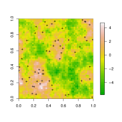
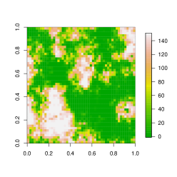
Figure 1: Maps of (a) the Gaussian process and (b) the intensity function of simulated dataset 1 considering a preferential sampling generating scheme.

The MCMC algorithm was run for 200,000 iterations with a burn-in of size 20,000. The posterior sample was constructed with a lag of 60, resulting in a 6,000 sample size. The convergence of the Markov chains was verified graphically through the posterior parameters trace plots (the plots are shown in the supplementary material). The exact model with preferential sampling will be denote by EPS, the discrete model with preferential sampling by DPS and the non preferential model by NPS.

Figure 2 shows the posterior densities of the parameters. Good parameter estimation is observed for most of the datasets, for all parameters, despite their modest sample sizes. The $\beta$ parameter was recovered well in half of the datasets and was underestimated in the rest, but showing a very substantial probability mass at positive values for all datasets. This means that the model was able to capture the sampling preferentiality present in the synthetic datasets.

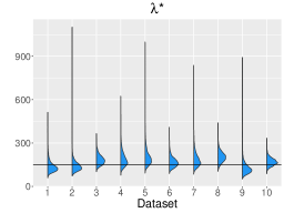
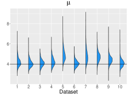
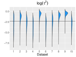
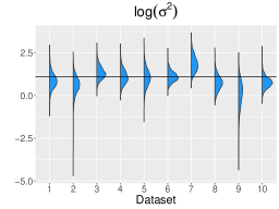
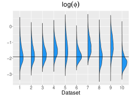
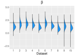
Figure 2: Posterior densities of the parameters of the EPS model for data simulated with preferential sampling. The horizontal line represents the true value of the parameter.

The parameters were also estimated using the non preferential model and results are showed in Figure 3. The mean parameter is overestimated in all datasets, as expected, to compensate for the lack of preferentiality in the model.

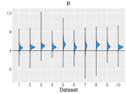
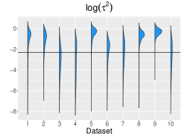
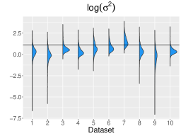
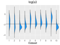
Figure 3: Posterior densities of the parameters of the NPS model for data simulated with preferential sampling. The horizontal line represents the true value of the parameter.

Two measures were considered to assess the predictive performance of the models: the mean absolute prediction error (MAPE) and the coverage ratio of credibility intervals (CRCI), given by

$$MAPE = \frac{1}{n_{p}}\sum_{i=1}^{n_{p}}|\hat{Y}(x_{i})-y(x_{i})|,$$

$$CRCI_{\alpha} = \frac{1}{n_{p}}\sum_{i=1}^{n_{p}}\mathbbm{1}\{y(x_{i})\in CI(Y(x_{i}),\alpha)\},$$

where $CI(Z,\alpha)$ stands for a $(1-\alpha)$ predictive credibility interval for $Z$, $\hat{Y}(x_{i})$ and $y(x_{i})$ are the respective mean of the predictive distribution and observed value of $Y$ at the unobserved location $x_{i}$ and $n_{p}$ is the size of the vector of unobserved locations for prediction, for $i=1,...,n_{p}$. Better models should present CRCI levels closer to the nominal level $1-\alpha$.

A regular grid of size $30\times 30$ was considered and prediction was performed for both models. Figure 4 shows the result and, as expected, the PS model presented better predictive performance. Results for CRCI were obtained with $\alpha=0.05$ but similar results were obtained with credibility intervals of 90% and 99% (graphs are presented in the supplementary material). Thus, the EPS model proves to be the adequate route when preferentiality is present in the data.

Figure 4: Quality measures of prediction for EPS (continuous line) and NPS (dashed line) models for simulated data with preferential sampling.

3.2 Data without preferential sampling

It has just been shown that the exact model provided good results in the preferentiality context. Now, the quality of the exact model is verified in a non preferential context. 10 datasets were simulated under the traditional scenario of non-preferentiality and the sample size of each one is presented in Table 2. The same prior distributions of Section 3.1 were adopted.

Dataset	1	2	3	4	5	6	7	8	9	10
n	67	70	77	87	73	70	78	80	66	70

Table 2: Size of the simulated datasets without preferentiality.

The posterior densities of the parameters estimated by the exact model are presented in Figure 5. As can be observed, good estimation was obtained for all parameters. The posterior distribution of $\beta$ has most densities around the true value 0, indicating that the model was able to capture the non-preferentiality of the data.

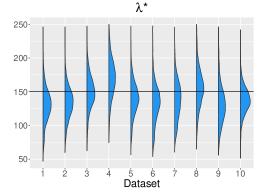
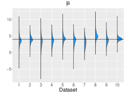
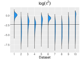
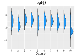
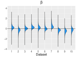
Figure 5: Posterior densities of the parameters of the EPS model for data simulated without preferential sampling. The horizontal line represents the true value of the parameter.

The quality of prediction was also compared for both models. It indicates that both models have similar performance in predicting data at unobserved locations when there is no preferential sampling (results are shown in the supplementary material).

These exercises suggest that little is lost by assuming preferentiality even when it is not present. Estimation and prediction results do not seem to suffer in the comparison. These results differ from those from the from previous section where wrongly assuming absence of preferentiality was shown to deteriorate the performance of the wrong model. In both cases, they show a robust performance of the EPS model in a variety of different scenarios.

3.3 Comparison of the exact and discrete models

The performance of the commonly used discretized approach was also assessed. A regular grid of size $15\times 15$ over the unit square was considered and the discrete model was constructed as in Ferreira and Gamerman (2015) (the description of the model can be viewed in the supplementary material). The datasets and prior distributions used here are the same of the Section 3.1.

Similar estimates were observed for $\lambda^{*}$, $\mu$ and $\beta$ in terms of parameter estimation. But better results for the variance and correlation parameters were obtained for the exact model (see the posterior densities in the supplementary material). Since the exact approach does not use approximations, the actual observed locations are used and simulations of points are made over the continuous region, providing better results.

The approaches were also compared in terms of prediction. Figure 6 shows those measures calculated for both models. The exact model provided better prediction measures in most of the datasets, which evidences the better performance of the exact methodology. Similar results of CRCI considering 90% and 99% are presented in the supplementary material, and basically confirm the results shown here.

Figure 6: Graphs of prediction quality measures of the process $Y$ performed by the EPS (continuous line) and the DPS (dashed line) models considering the simulated datasets with preferential sampling.

4 Application

In this section, two real datasets are analyzed to illustrate the findings of the present work. The first one is the radiation data in Germany, well known in the geostatistics literature as a dataset that does not present preferentiality (Dubois, 2005; Ingram et al., 2007). This data set is a good test for assessing the effectiveness of the exact preferential model in a context where no preferentiality was verified. The second one is the Galicia moss data, another well known dataset in literature that presents preferentiality in sampling (Fernández et al., 2000; Diggle et al., 2010; Dinsdale and Salibian-Barrera, 2019). This data is also analyzed with the discretized model, which enables the verification of the possible benefits of the exact approach over the approximated discretization.

4.1 Germany radiation data

The Radioactivity Environmental Monitoring (REM) developed a data platform with the aim to make data of radioactive monitoring available for researchers. The automatic mapping from updated data becomes useful since its information updates occurs almost in real time. Then, the REM group managed an web exercise, the Spatial Interpolation Comparison (SIC) of 2004, in which participants could predict data using part of a real dataset. For further information, see Dubois and Galmarini (2005). The data contain measures of mean rates of gamma radiation in Germany and consists in 1008 monitoring locations, in which only 200 chosen randomly location were provided. The competition participants should perform prediction for the remaining 808 sites.

The variogram in Figure 7 presents points out of the simulated envelope (this was made by random permutations of data fixing its locations), indicating the presence of spatial correlation. The exponential correlation function was considered and its range is equal to 3$\phi$ (Diggle and Ribeiro, 2007). Thus, through the empirical range (about 6) indicated in the variogram, the correlation parameter $\phi$ was fixed to be equal 2.

Figure 7: Omnidirecional variogram and simulated envelope for radiation data in Germany.

Data was analyzed with EPS and NPS models. The $\lambda^{*}$ parameter was truncated in $500/|B|$, $B$ is the window considered of the region, indicating that the maximum mean number of points of the $W$ process was set to 500. The following prior distributions were assumed: $\lambda^{*}\sim Gamma(0.001,0.001)$, $\mu\sim N(0,10^{6})$, $\tau^{2}\sim IG(0.001,0.001)$, $\sigma^{2}\sim IG(0.001,0.001)$ and $\beta\sim N(0,1)$. The convergence of the Markov chains was verified through graphical analysis (see supplementary material).

Table 3 shows summary measures of the posterior densities of parameter for both models. The estimation of parameters that are common to both models is similar, as expected. This is also confirmed with the $\beta$ estimation, with its estimated value near 0 and the 95% credibility intervals containing 0. In Figure 8, all posterior densities are unimodal and they are similar for both models considering the common parameters.

Model	Parameter	Mean	Median	SE	CI(95%)
EPS	$\lambda^{*}$	17.012	17.004	1.479	[ 14.026 ; 20.015 ]
	$\mu$	94.670	94.571	7.795	[ 80.165 ; 110.662 ]
	$\tau^{2}$	75.979	75.294	12.848	[ 53.320 ; 104.075 ]
	$\sigma^{2}$	261.953	256.650	69.170	[ 148.104 ; 418.897 ]
	$\beta$	-0.084	-0.082	0.111	[ -0.315 ; 0.130 ]
NPS	$\mu$	94.669	94.437	8.496	[ 78.233 ; 112.714 ]
	$\tau^{2}$	76.194	75.960	12.378	[ 53.181 ; 101.849 ]
	$\sigma^{2}$	259.590	251.229	67.085	[ 155.017 ; 403.486 ]

Table 3: Summary measures of the posterior density distributions of the parameters of the EPS and NPS models for radiation data in Germany.

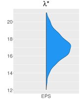
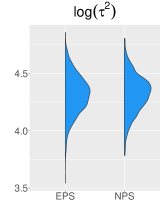
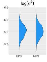
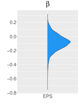
Figure 8: Posterior densities of model parameters for radiation data in Germany.

The process $Y$ was predicted at the 808 remaining sites of the dataset and MAPE was calculated. The MAPE values obtained for the EPS and NPS model were quite similar with respective values 9.073 and 9.075. The NPS model is more adequate since data does not shows preferentiality. But, the results indicates that the EPS model performs as well as the NPS model in this context. These results corroborate the findings from the previous section, which indicate that there is no substantial loss in performance by using the EPS model for non preferential data. Figure 9 shows the predicted maps of data over a $30\times 30$ regular grid and similar maps are observed between the models, with lower predicted errors corresponding to the EPS model. Thus, the exact model showed good performance even in the non preferential sampling context with a real dataset scenario.

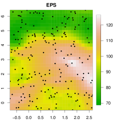
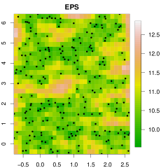
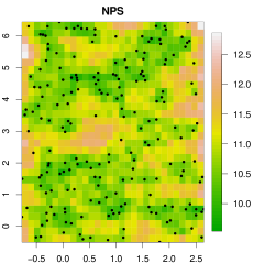
Figure 9: Predicted maps of $Y$ (first column) and predicted errors (second column) for radiation data in Germany.

4.2 Galicia moss data

The data consists of measures of lead concentrations in samples of moss in Galicia, northern Spain. The uptake of heavy metals in mosses occurs mainly from atmospheric deposition, which turns mosses into biomonitoring of pollution. The study was conducted over a number of years but here we concentraqted on the analysis of the data collected in October 1997. Figure 10 shows the sampling design. The choice of sampling locations was conducted more intensively in subregions where high lead concentration was expected, turning this sampling design potentially preferential. As a result, this data set is frequently used as an example of sampling preferentiality in the geostatistics literature.

Figure 10: Sampling locations of Galicia moss data.

Therefore, this data was analyzed only with the models that contemplate preferentiality EPS and DPS in order to assess the possible effect of taking an exact stand at preferentiality. A regular grid of $15\times 15$ was considered for the DPS model. The following prior distributions were adopted: $\lambda^{*}\sim Gamma(0.001,0.001)$, $\mu\sim N(0,10^{6})$, $\tau^{2}\sim IG(0.001,0.001)$, $\sigma^{2}\sim IG(0.001,0.001)$, $\phi\sim Gamma(2,4)$, and $\beta\sim N(0,1)$. The convergence of the Markov chains was verified through graphical analysis (see supplementary material).

Table 4 shows summary measures and Figure 11 presents the posterior densities of parameter for the models. Estimation of $\beta$ in both models indicated large concentration of posterior probability over negative values and basically not including 0. These results strongly indicate that there could be preferentiality in this survey, in line with previous analyses of this dataset. The estimation with the DPS model indicate higher values of the nugget effect and lower values for $\sigma^{2}$. The effect of the discretization can also be seen in the estimation of $\beta$. It is clearly different from 0 for both the exact and the discretized models, but with dampened values for the latter in comparison to the values obtained with the exact PS model.

Model	Parameter	Mean	Median	SE	CI(95%)
EPS	$\lambda^{*}$	64.843	59.330	24.640	[ 34.449 ; 128.702 ]
	$\mu$	1.576	1.580	0.177	[ 1.196 ; 1.917 ]
	$\tau^{2}$	0.135	0.133	0.048	[ 0.046 ; 0.237 ]
	$\sigma^{2}$	0.245	0.203	0.184	[ 0.031 ; 0.686 ]
	$\phi$	0.615	0.533	0.332	[ 0.212 ; 1.486 ]
	$\beta$	-1.458	-1.394	0.441	[ -2.495 ; -0.763 ]
DPS	$\lambda^{*}$	65.520	58.210	33.395	[ 25.093 ; 150.663 ]
	$\mu$	1.423	1.423	0.132	[ 1.159 ; 1.677 ]
	$\tau^{2}$	0.198	0.193	0.044	[ 0.128 ; 0.298 ]
	$\sigma^{2}$	0.081	0.052	0.093	[ 0.007 ; 0.331 ]
	$\phi$	0.992	0.944	0.402	[ 0.368 ; 1.932 ]
	$\beta$	-0.826	-0.803	0.347	[ -1.582 ; -0.229 ]

Table 4: Summary measures of the posterior densities of the parameters of EPS and DPS models for the Galicia moss data in 1997.

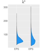
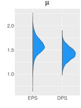
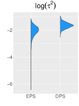
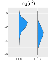
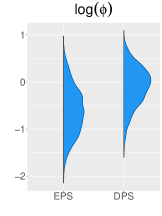
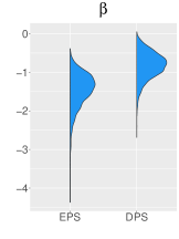
Figure 11: Posterior densities of model parameters for Galicia moss data in 1997.

Figure 12 shows the predicted maps in Galicia region over a regular grid of $30\times 30$. The DPS model provided a shorter range of predicted values and lower prediction in regions without observations in comparison to the EPS model.

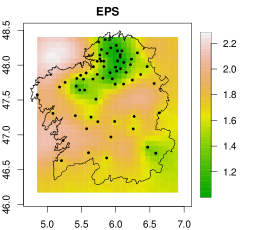
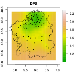
Figure 12: Predicted map of $Y$ of Galicia moss data in 1997 considering the EPS and DPS models.

A cross validation was performed to compare the quality of the predictions of the EPS and DPS models. Results are presented in Table 5. The PPD measure corresponds to the sum of the log posterior predicted densities at the true value of the removed observation, summed up for all observations. The EPS model provided better results in all measures, which evidences superior performance of the exact approach in relation to the discretized approach.

Model	MAPE	PPD	CRCI
			90%	95%	99%
EPS	0.388	-41.023	0.921	0.968	0.984
DPS	0.415	-45.170	0.937	0.984	1.000

Table 5: Results of the cross validation exercise to the Galicia moss data.

5 Discussion

It is well known that inference can be incorrect if sampling preferentiality is ignored in the analysis. Most proposals to address preferentiality in geostatistics make use of model approximation. This paper proposed a methodology to make exact inference for the geostatistical model under preferential sampling without model approximations.

Results showed that the exact model provided good parameter estimation and prediction in the preferential and non preferential sampling context. In all simulated datasets, the estimation values of the preferentiality parameter $\beta$ reflected the correct context of the data: values different from zero for the former and values around zero for the latter. It has also been shown that better results were obtained with the exact model in comparison against the approximated model.

The proposed model was tested in two real datasets. The first dataset is well known in the geostatistics literature as an example of non-preferential sampling. In this situation, results showed that the exact model provided similar estimation and the posterior distribution indicated that the model was able to identify the non-preferentiality of the data. Also, similar prediction results were obtained with the proposed model, which evidences the robustness of the exact approach even in the non-preferential context. The second dataset is also well known in the geostatistics literature but as an example of preferential sampling. Our results show that the models were capable to identify the preferentiality of the data but, more importantly, the exact model outperformed the discretized model, confirming results obtained with simulations.

All exercises were based on the exponential correlation function. Other functions can be easily accomodated with the appropriate modification of the corresponding step in the MCMC for sampling unknown hyperparameters of the correlation function.

Thus, there are strong reasons to believe that the proposed methodology can be used not only to correct the bias of the preferential sampling, but also to verify if it exists in the data under analysis. Moreover, generalizations of the model can be constructed to allow the analysis of non-Gaussian data. This can be done by changing the distribution of the latent process and/or the response process. Situations where outliers are present in data, for example, need distributions that are more robust than the Gaussian and this feature can be of interest.

The assumption of gaussianity of the response can be easily relaxed to allow for other sampling data distributions. This can be readily accommodated for a large number of distributions: scale mixtures of gaussian (including t-Student), bernoulli and Poisson are just a few examples. Different augmentation schemes around the gaussian specification were designed for each one of them (see for respective details Carlin et al. (1992), Albert and Chib (1993), Frühwirth-Schnatter and Wagner (2006)). All it takes is an additional, inexpensive draw associated with each observed response $Y$.

Finally, the methodology has substantial computational cost directly associated with handling high-dimensional multivariate normal distributions. Simulation of these distributions will be required and the computation becomes slow when the number of observed locations is large. This is a well known problem in the spatial statistics literature and substantial amount of work was generated to provide adequate solutions for these scenarios (see Banerjee et al. (2008); Kaufman et al. (2008); Lindgren et al. (2011); Datta et al. (2016)). Improving the computational efficiency of our methodology is an important extension of this work.
 

Supplementary Material

Supplementary material for the article Exact Bayesian Geostatistics under Preferential Sampling. This supplementary material provides proofs for some of the results and the remainder of the computational results of the simulated study and the application.

ACKNOWLEDGEMENTS

The authors acknowledge the partial financial support from CAPES-Brazil and CNPQ-Brazil. The work is based on the doctoral thesis of the first author, developed under supervision of the second author. Both authors thank the hospitality and the fruitful working environment of the Graduate Program in Statistics at UFMG.

References

- Albert and Chib (1993) Albert, J. H. and Chib, S. (1993), “Bayesian analysis of binary and polychotomous response data,” Journal of the American Statistical Association, 88, 669–679.
- Banerjee et al. (2008) Banerjee, S., Gelfand, A. E., Finley, A. O., and Sang, H. (2008), “Gaussian predictive process models for large spatial data sets,” Journal of the Royal Statistical Society: Series B, 70, 825–848.
- Butler and Moffitt (1982) Butler, J. S. and Moffitt, R. (1982), “A computationally efficient quadrature procedure for the one-factor multinomial Probit model,” Econometrica, 50, 761–764.
- Carlin et al. (1992) Carlin, B. P., Polson, N. G., and Stoffer, D. S. (1992), “A Monte Carlo approach to nonnormal and nonlinear state-space modeling,” Journal of the American Statistical Association, 87, 493–500.
- Datta et al. (2016) Datta, A., Banerjee, S., Finley, A. O., and Gelfand, A. E. (2016), “Hierarchical nearest-neighbor Gaussian process models for large geostatistical datasets,” Journal of the American Statistical Association, 111, 800–812.
- Diggle and Ribeiro (2007) Diggle, P. and Ribeiro, P. (2007), Model-based Geostatistics., Springer.
- Diggle et al. (2010) Diggle, P. J., Menezes, R., and Su, T. (2010), “Geostatistical inference under preferential sampling,” Journal of the Royal Statistical Society: Series C, 59, 191–232.
- Dinsdale and Salibian-Barrera (2019) Dinsdale, D. and Salibian-Barrera, M. (2019), “Methods for preferential sampling in geoestatistics,” Journal of the Royal Statistical Society: Series C, 68, 181–198.
- Dubois (2005) Dubois, G. (2005), “SIC2004: an exercise for automatic mapping in emergencies,” Geophysical Research Abstracts.
- Dubois and Galmarini (2005) Dubois, G. and Galmarini, S. (2005), “Introduction to the spatial interpolation comparison (SIC) 2004 exercise and presentation of the datasets,” Applied Gis, 1.
- Eddelbuettel and François (2011) Eddelbuettel, D. and François, R. (2011), “Rcpp: Seamless R and C++ integration,” Journal of Statistical Software, 40, 1–18.
- Fernández et al. (2000) Fernández, J., Rey, A., and Carballeira, A. (2000), “An extended study of heavy metal deposition in Galicia (NW Spain) based on moss analysis,” The Science of the Total Enviroment, 254, 31–44.
- Ferreira and Gamerman (2015) Ferreira, G. and Gamerman, D. (2015), “Optimal design in geostatistics under preferential sampling (with discussion),” Bayesian Analysis, 10, 711 – 735.
- Frühwirth-Schnatter and Wagner (2006) Frühwirth-Schnatter, S. and Wagner, H. (2006), “Auxiliary mixture sampling for parameter-driven models of time series of counts with applications to state space modelling,” Biometrika, 93, 827–841.
- Gelfand et al. (2012) Gelfand, A. E., Sahu, S. K., and Holland, D. M. (2012), “On the effect of preferential sampling in spatial prediction,” Environmetrics, 23, 565–578.