Stealthy Measurement-Aided Pole-Dynamics Attacks with Nominal Models

Abstract

When traditional pole-dynamics attacks (TPDAs) are implemented with nominal models, model mismatch between exact and nominal models often affects their stealthiness, or even makes the stealthiness lost. To solve this problem, our current paper presents a novel stealthy measurement-aided pole-dynamics attacks (MAPDAs) method with model mismatch. Firstly, the limitations of TPDAs using exact models are revealed, where exact models help ensure the stealthiness of TPDAs but model mismatch severely influences its stealthiness. Secondly, to handle model mismatch, the proposed MAPDAs method is designed by using a model reference adaptive control strategy, which can keep the stealthiness. Moreover, it is easier to implement as only the measurements are needed in comparison with the existing methods requiring both the measurements and control inputs. Thirdly, the performance of the proposed MAPDAs method is explored using convergence of multivariate measurements, and MAPDAs with model mismatch have the same stealthiness and similar destructiveness as TPDAs. Specifically, MAPDAs with adaptive gains will remain stealthy at an acceptable detection threshold till destructiveness occurs. Finally, experimental results from a networked inverted pendulum system confirm the feasibility and effectiveness of the proposed method.

, , , ,

1 Introduction

Networked control systems (NCSs) [Zhang et al., 2020], [Zhang & Peng, 2019], [Shen & Petersen, 2018] deploy communication networks to exchange information between physical entities such as plants, sensors and controllers. Compared with traditional control systems, NCSs eliminate unnecessary wiring, reduce system complexity and cost, and improve system performance. However, the usage of networks makes NCSs open to the outer space and thus be vulnerable to cyber attacks. Recently, there are several attack incidents (e.g., Stuxnet-like attacks on nuclear facilities [Tian et al., 2020] and Blackenergy on power grids [Saxena et al., 2021]). In this context, it is not surprising that seeking promising solutions to various attacks has attracted wide attention in the community.

The majority of efforts have been made to address a critical question: What degree of attacks can a system bear with the stealthiness before destructiveness is met? Destructiveness means that attacks intentionally drive system state to cross admissible limit, whilst the stealthiness indicates that attacks hide from detectors. There are many types of stealthy attacks, including model-free attacks (e.g., replay attacks [Xu et al., 2021], optimal linear attacks [Guo et al., 2017] and switching location attacks [Liu et al., 2017]) and model-based attacks (e.g., undetectable linear attacks [Song et al., 2019], feedback-loop covert attacks [Mikhaylenko & Zhang, 2021], zero-dynamic attacks [Teixeira et al., 2015] and pole-dynamics attacks [Kim et al., 2021]). Unlike model-free attacks, model-based attacks rely on a deliberate model to design attacks. A review of recent model-based attacks has been carried out in Section 1.1 of the supplementary materials [Du et al., 2022]. When an exact model has been known, model-based attacks can be of the stealthiness whether or not they engage the measurements, control inputs or both.

Table 1: Comparison between the existing construction methods of stealthy attacks and the proposed method.

References	Name	Type	Model Required	Type of Plant	MR1	CIR2
[Song et al., 2019]	ULAs3	MBAs4	Exact model	Arbitrary	✗5	✗
[Mikhaylenko & Zhang, 2021]	FLCAs6	MBAs	Exact model	Arbitrary	✗	✗
[Teixeira et al., 2015]	ZDAs7	MBAs	Exact model	Non-minimum phase	✗	✗
[Kim et al., 2021]	PDAs	MBAs	Exact model	Unstable pole-dynamics	✗	✗
[Li & Yang, 2018]	DFLCAs8	IMBAs9	No model	Arbitrary	✔10	✔
[Li et al., 2019]	TLCAs11	IMBAs	No model	Arbitrary	✔	✔
[Park et al., 2019]	RZDAs12	IMBAs	Nominal model	Non-minimum phase	✔	✔
[Jeon & Eun, 2019]	RPDAs13	IMBAs	Nominal model	Unstable pole-dynamics	✔	✔
The proposed method	MAPDAs	IMBAs	Nominal model	Unstable pole-dynamics	✔	✗
1Measurement required. 2Control input required. 3Undetectable linear attacks. 4Model-based attacks.
5Not required. 6Feedback-loop covert attacks. 7Zero-dynamics attacks.8Data-driven FLCA. 9Improved MBA.
10Required. 11Data-driven two-loop covert attacks. 12Robust ZDA. 13Robust PDA.

However, it is unrealistic to retrieve exact models used by the attacker or defender in many industrial control systems, leading to model mismatch between exact and nominal models. With nominal models, model-based attacks may lose their stealthiness. This brings a consequent question: Are model-based attacks helpless against model mismatch? The answer is no, and there actually are some improved model-based attacks methodologies, e.g., data-driven feedback-loop/two-loop covert attacks [Li & Yang, 2018], [Li et al., 2019], robust zero-dynamics attacks [Park et al., 2019] and robust PDAs [Jeon & Eun, 2019]. A review of the existing improved model-based attacks techniques will be carried out in Section 1.1 of the supplementary materials [Du et al., 2022].

Although the existing improved model-based attacks methods have provided promising performance, control inputs are indispensable to the outcome of these methods, e.g., both control inputs and the measurements are required to design the attack mechanisms. This brings a new question: Can improved model-based attacks methods without using control inputs be working against model mismatch between exact and nominal models? In a practical sense, there exist several vulnerable-sensor-network-only NCSs (especially Internet of Things applications [Lyu et al., 2018]) where a vulnerable wireless network may be used to link the sensors and the controller, and reliable cable networks may be used to connect the controller with the plant. Therefore, from the perspective of a defender, the above question is equivalent to this one: Are vulnerable-sensor-network-only NCSs safe enough from these stealthy attacks thanks to model mismatch between exact and nominal models?

Motivated by the above observations, the following challenges and difficulties will be addressed:

1. Traditional pole-dynamics attacks (TPDAs) are implemented with exact models, which is impractical for some attackers. They have no choice but to use nominal models to design attacks, however model mismatch between exact and nominal models may lead to decline or even loss of stealthiness. Therefore, how to reveal the limitations of TPDAs with nominal models is the first challenge.

2. Some popular techniques (e.g., robust control and data driven) can be employed to improve the stealthiness of TPDAs with nominal models requiring complete and accurate measurements and control inputs. It is difficult for the attacker to launch attacks by obtaining these signals especially in vulnerable-sensor-network-only NCSs. Therefore, how to propose a new attack method without control input is the second challenge.

3. The existing improved model-based attacks (e.g., robust zero-dynamics attacks and robust PDAs) have been mainly designed for single-input-single-output systems, which have rarely been implemented in multiple-input-multiple-output (MIMO) systems. When the above proposed attack method is employed in MIMO systems, identification of stealthiness and destructiveness is the third challenge.

To deal with the above challenges and difficulties, this paper presents a stealthy measurement-aided pole-dynamics attacks (MAPDAs) method with model mismatch for uncertain vulnerable-sensor-network-only NCSs. Comparative analysis between the existing methods and the proposed method is listed in Table 1. The existing methods are mainly based on an exact model or a nominal model but require complete and accurate control inputs, but this paper has revealed the limitations of TPDAs, proposed the new MAPDAs method with model mismatch, and provided the proof of stealthiness and destructiveness of MAPDAs. The main contributions of this paper are summarized as follows:

1. The limitations of TPDAs using exact models are revealed, where exact models can ensure the stealthiness of TPDAs but model mismatch between the exact and nominal models may cause TPDAs to lose the stealthiness.

2. To handle model mismatch, a new MAPDAs method is proposed using a model reference adaptive control strategy, which can keep the stealthiness. Moreover, it is easier to implement as only the measurements are needed in comparison with the existing methods requiring both the measurements and control inputs.

3. The stealthiness and destructiveness of the proposed MAPDAs in MIMO systems is explored by investigating the convergence of multivariate measurements, where MAPDAs with model mismatch have the same stealthiness and similar destructiveness as TPDAs. Specifically, MAPDAs with adaptive gains will remain stealthy at an acceptable detection threshold till destructiveness occurs.

The reminder of this paper is organized as follows. Section 2 is problem formation, where the limitations of TPDAs with model mismatch are discussed. Section 3 describes the proposed MAPDAs and analyzes the performance. Section 4 provides the experiments where TPDAs and MAPDAs are embedded in the practical networked inverted pendulum visual servo system (NIPVSS), followed by the conclusions made in Section 5.

Remark 1.

Due to space constraints, some necessary contents are placed in the supplementary materials [Du et al., 2022].

Notation. For a matrix $P$, $P>0$ denotes that $P$ is positive definite symmetric. The one vector (all elements are 1) is denoted by $\textbf{1}_{n}\in\mathbb{R}^{n}$. Table A.1 in Section 1.2 of supplementary materials [Du et al., 2022] summarizes the notations most frequently used throughout the rest of the paper.

2 Problem Formulation

2.1 NCSs under TPDAs with Exact Model

The framework of NCSs for TPDAs with exact auxiliary model (i.e., exact model) is shown in Fig. 1. Firstly, the sensor obtains the measurement $x(t)$ from the plant. Then, $x(t)$ will be transmitted to the estimator and controller via networks, becoming $x_{a}(t)$ due to injection of attack signals $a(t)$ from possible TPDAs with exact auxiliary model. Using $x_{a}(t)$, the controller calculates control input $u(t)$ that is sent to the actuator to stabilize the plant and the estimator judges whether or not there exists an attack, and if there is an attack, the alarm will be triggered.

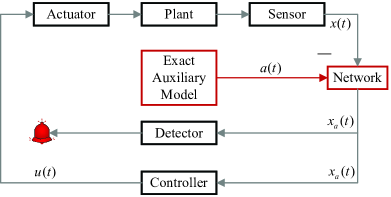
Figure 1: Framework of NCSs for TPDAs with exact auxiliary models.

Remark 2.

Fig. 1 shows the framework of NCSs for TPDAs with exact auxiliary model, where the construction of TPDAs adopts exact auxiliary model (3) that only needs the matrix $A$ of physical system (1) and does not use $x(t)$, see [Kim et al., 2021], [Jeon & Eun, 2019]. However, when there exists model mismatch between exact auxiliary model and nominal model (i.e., the attackers can not obtain exact auxiliary model), $x(t)$ and $u(t)$ have been applied to constructing model-based attacks for the stealthiness. Thus, $u(t)$ needs to be connected into exact auxiliary model box in this case, see [Li & Yang, 2018], [Li et al., 2019], [Park et al., 2019], [Jeon & Eun, 2019].

Consider continuous linear time-invariant (LTI) plant

$$\dot{x}(t) =Ax(t)+Bu(t),\hfill$$ (1)

$$z(t) =Cx(t),\hfill$$ (2)

where $x(t)\in\mathbb{R}^{p}$ is system state and the measurement, $u(t)\in\mathbb{R}^{m}$ is control input, $z(t)\in\mathbb{R}^{q}$ is controlled output, and $A$, $B$, and $C$ are constant matrices with appropriate dimensions. Without loss of generality, it is considered that (1) is controllable.

System state $x(t)$ will be transmitted to the controller of TPDAs via networks. TPDAs can maintain a continuous exact auxiliary model ${\mathcal{A}_{c,t}}(A)$ [Kim et al., 2021], [Jeon & Eun, 2019]:

$${{\dot{x}}_{\rm eam}}(t) =A{x_{\rm eam}}(t),\hfill$$ (3a)

$$a(t) ={x_{\rm eam}}(t),\hfill$$ (3b)

where $x_{\rm eam}(t)$ and $a(t)$ are the state and the output of $\mathcal{A}_{c,t}(A)$. In a network, $a(t)$ may be subtracted from $x(t)$, and thus the network output becomes

$$x_{a}(t)=x(t)-a(t).$$ (4)

Using $x_{a}(t)$, the controller calculates the control input

$$u(t)=Kx_{a}(t),$$ (5)

where $K$ is the controller gain and has been designed to make $\Phi:=A+BK$ stable (i.e., the eigenvalues of $\Phi$ are located on the closed left half-plane). Then, $u(t)$ will be sent to the actuator for stabilizing the plant.

To detect attacks, the common norm-based test is performed by the detector, i.e., if there is

$$\left\|{{x_{a}}(t)}\right\|<\epsilon,$$ (6)

where $\epsilon>0$ is a user-defined threshold, it means that there is no attack, otherwise, attacks emerge.

Remark 3.

The threshold $\epsilon$ of the detector (6) is the key to examine the validity of attack detection. The existing threshold selection methods generally include statistical analysis [Heydt & Graf, 2010], theoretical derivation [Mo & Sinopoli, 2009], machine learning [Zhao et al., 2020], etc. To determine the proper threshold, the method of statistical analysis is used in Section 4.

To analyse the performance of attacks, the definitions of stealthiness and destructiveness in time period $\mathcal{T}:=[t_{0},t_{f}]$ of attacks are given in the following, where $t_{0}$, $t_{f}$ are initial and finishing instants of attacks, respectively.

Definition 1 ($\epsilon$-stealthiness).

(cf. [Kung et al., 2017]) An attack is said to be with $\epsilon$-stealthiness on the detector in $\mathcal{T}$ when (6) for $t\in\mathcal{T}$ always holds.

Definition 2 ($\xi$-destructiveness).

(cf. [Park et al., 2019]) An attack is said to be with $\xi$-destructiveness on the controlled output $z(t_{f})$ if

$$\left\|z(t_{f})\right\|\geqslant\xi,$$ (7)

where $\xi$ is the admissible state limit. Specifically, $\left\|z(t)\right\|<\xi$ for $t\in\mathcal{T}$ will run under control and $\left\|z(t)\right\|\geqslant\xi$ for $t\in\mathcal{T}$ is actively out of control (e.g., takes active protection measures) to avoid possible severe accidents.

It is well believed that an ideal attack in $\mathcal{T}$ should be with both $\xi$-destructiveness and $\epsilon$-stealthiness. We may witness a more dangerous scenario where a quasi-ideal attack is with $\epsilon$-stealthiness and with no $\xi$-destructiveness in $\mathcal{T}$, but the controlled output is driven very close to $\xi$. A quasi-ideal attack could be on the synchronous machines [Endrejat & Pillay, 2011], where the attack will not make rotation rates of synchronous machines cross the admissible limit, but it pushes the rotation rate to be high. This will remarkably shorten the life of synchronous machines and even cause accidents. For simplicity, our current paper only focuses on ideal attacks.

2.2 Performance of TPDAs with Exact Auxiliary Models

Based on the above NCSs under TPDAs, the definitions and impact analysis of TPDAs with $\mathcal{A}_{c,t}(A)$ (3) in [Jeon & Eun, 2019], the stealthiness and destructiveness of TPDAs with $\mathcal{A}_{c,t}(A)$ (3) are presented in the following Theorem 1.

Theorem 1.

Considering system (1)-(5) under TPDAs with $\mathcal{A}_{c,t}(A)$ (3), if $\Phi$ is stable, $A$ is unstable (i.e., at least one of eigenvalues of $A$ is located on the open right half-plane), and $x_{eam}(t_{0})$ does not satisfy the item (i) or (ii) of Lemma A.1 in Section 2.1 of the supplementary materials [Du et al., 2022], then

$$\exists\epsilon,\left\|{{x_{a}}(t)}\right\|<\epsilon,t\in[{t_{0}},\infty).$$ (8)

The norm of system state becomes unbounded, i.e.,

$$\mathop{\lim}\limits_{t\to\infty}\left\|x(t)\right\|\to\infty.$$ (9)

The proof is given in Section 2.2 of the supplementary materials [Du et al., 2022].

Remark 4.

For Theorem 1, there possibly exist two cases for TPDAs with $\mathcal{A}_{c,t}(A)$ (3), i.e., $\epsilon>{\sup}_{\rm eam}\left\|{x_{a}}\right\|$ (${\sup}_{\rm eam}\left\|{x_{a}}\right\|$ represents the upper bound of $\left\|x_{a}(t)\right\|$ under TPDAs with $\mathcal{A}_{c,t}(A)$ (3)) and $\epsilon\leqslant{\sup}_{\rm eam}\left\|{x_{a}}\right\|$, which is shown in Fig. A.1(a) of Section 2.3 in the supplementary materials [Du et al., 2022]. Therefore, for a given $\epsilon$, when a small enough ${\sup}_{\rm eam}\left\|{x_{a}}\right\|$ is selected, TPDAs with $\mathcal{A}_{c,t}(A)$ (3) can be with $\xi$-destructiveness and $\epsilon$-stealthiness in $\mathcal{T}$.

Remark 5.

For Lemma A.1 in Section 2.1 of the supplementary materials [Du et al., 2022], we examine whether or not the initial value of ${x_{{\rm eam},i}}({t_{0}})$ [i.e., $x_{{\rm eam},i}(t_{0})$ corresponding to the $i^{th}$ eigenvalue $\lambda_{i}$ of the matrix $A$, $i=1,\ldots,p$] equals to zero. There are two cases for $x(t)$: (1) If $x_{\rm eam}(t_{0})$ satisfies the initial condition in Lemma A.1, $\mathop{\lim}\limits_{t\to\infty}{x_{{\text{eam}}}}(t)=0$ even if $A$ is unstable. Furthermore, according to (3), (4) and (A.3) in Section 2.2 of the supplementary materials [Du et al., 2022], $\mathop{\lim}\limits_{t\to\infty}x(t)=0$ so that (9) will not hold; (2) If $x_{\rm eam}(t_{0})$ does not satisfy the initial condition in Lemma A.1, $\mathop{\lim}\limits_{t\to\infty}\left\|{{x_{\rm eam}}(t)}\right\|\to\infty$ as $A$ is unstable. Furthermore, according to (3), (4) and (A.3), $\mathop{\lim}\limits_{t\to\infty}\left\|{x(t)}\right\|\to\infty$, and (9) in Theorem 1 holds.

2.3 Limitation of TPDAs with Nominal Models

Although the above stealthiness and destructiveness of TPDAs with $\mathcal{A}_{c,t}(A)$ (3) look promising, it is unrealistic to obtain the exact model for the attacker (even for the defender). When the attacker only knows the nominal model of uncertain NCSs (i.e., the nominal model $A_{n}$ of $A$), they have to perform TPDAs with a continuous nominal auxiliary model ${\mathcal{A}_{c,t}}({A_{n}})$

$${{\dot{x}}_{{\text{nam}}}}(t) ={A_{n}}{x_{{\text{nam}}}}(t),\hfill$$ (10a)

$$a(t) ={x_{{\text{nam}}}}(t),\hfill$$ (10b)

According to impact analysis of TPDAs with $\mathcal{A}_{c,t}(A)$ (3) in [Jeon & Eun, 2019], the limitation of TPDAs with $\mathcal{A}_{c,t}(A_{n})$ (10) is presented in the following Theorem 2.

Theorem 2.

Considering the system (1), (2), (4), (5) under TPDAs with $\mathcal{A}_{c,t}(A_{n})$ (10), if $\Phi$ is stable, $A_{n}$ is unstable, and $x_{\rm nam}(t_{0})$ does not satisfy the item (i) or (ii) of Lemma A.2 in Section 2.5 of the supplementary materials [Du et al., 2022], then

$$\mathop{\lim}\limits_{t\to\infty}\left\|x_{a}(t)\right\|\to\infty.$$ (11)

The norm of system state becomes unbounded, i.e., (9).

The proof is given in Section 2.4 of the supplementary materials [Du et al., 2022].

Remark 6.

For Theorem 2, there possibly exist two case for TPDAs with $\mathcal{A}_{c,t}(A_{n})$ (10), i.e., $\epsilon>\left\|{x_{a}(t_{f})}\right\|$ and $\epsilon\leqslant\left\|{x_{a}(t_{f})}\right\|$ ($t_{f}$ is finishing instant of attacks), which is shown in Fig. A.1(b) of Section 2.3 in the supplementary materials [Du et al., 2022]. Therefore, when a small $\epsilon$ is selected, TPDAs with $\mathcal{A}_{c,t}(A_{n})$ (10) are with $\xi$-destructiveness but with no $\epsilon$-stealthiness in $\mathcal{T}$.

Remark 7.

For Lemma A.2 in Section 2.5 of the supplementary materials [Du et al., 2022], we have analysed whether or not the initial value of $x_{{\rm nam},i}(t_{0})$ (i.e., $x_{{\rm nam},i}(t_{0})$ corresponding to the $i^{th}$ eigenvalue $\lambda_{n,i}$ of the matrix $A_{n}$) equals to zero. There are two cases for $x_{a}(t)$: (1) If $x_{\rm nam}(t_{0})$ satisfies the initial condition in Lemma A.2, $\mathop{\lim}\limits_{t\to\infty}{x_{\rm nam}}(t)=0$ even if $A_{n}$ is unstable. Furthermore, according to (10), (4) and (A.5) in Section 2.4 of the supplementary materials [Du et al., 2022], $\mathop{\lim}\limits_{t\to\infty}{{x_{a}}(t)}=0$ so that (11) will not hold; (2) If $x_{\rm nam}(t_{0})$ does not satisfy the initial condition in Lemma A.2, $\mathop{\lim}\limits_{t\to\infty}\left\|{{x_{\rm nam}}(t)}\right\|\to\infty$ because $A_{n}$ is unstable. Furthermore, according to (10), (4) and (A.5), $\mathop{\lim}\limits_{t\to\infty}\left\|{{x_{a}}(t)}\right\|\to\infty$, and (11) in Theorem 2 holds.

Up to now, we understand the limitations of TPDAs with nominal models, i.e., TPDAs will be with $\xi$-destructiveness but with no $\epsilon$-stealthiness in $\mathcal{T}$. In the next section, to cope with this problem, we will present a measurements and adaptive control based method into the attacks.

3 Measurement-Aided Pole-Dynamics Attacks

We have analysed NCSs under TPDAs and the limitations of TPDAs with nominal models in the previosu sections. To solve the problem, a stealthy MAPDAs method using measurements and an adaptive auxiliary model will be designed and discussed.

3.1 Design of MAPDAs

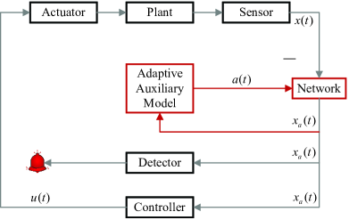
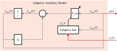
Figure 2: (a) Framework of NCSs under MAPDAs with an adaptive auxiliary model. (b) Framework of an adaptive auxiliary model.

The framework of NCSs under MAPDAs with an adaptive auxiliary model is shown in Fig. 2(a) and the framework of adaptive auxiliary model is shown in Fig. 2(b). Firstly, the sensor collects $x(t)$ from the plant. Then, $x(t)$ will be transmitted to the detector and controller via network, becoming $x_{a}(t)$ due to possible attacks. The attacker obtains $x_{a}(t)$ and uses it to construct adaptive auxiliary model with state $x_{\rm aam}(t)$ and output $a(t)$, where $x_{a}(t)$ and $x_{\rm aam}(t)$ are used to produce adaptive gain $F_{a}(t)$ based on the designed adaptive laws, and $F_{a}(t)$ is used to update $x_{\rm aam}(t)$ and $a(t)$. Using $x_{a}(t)$, the controller calculates $u(t)$ that is sent to the actuator to stabilize the plant and the estimator scrutinizes whether or not there is an attack, and if there is an attack, the alarm will be triggered.

Consider continuous LTI plant (1) and (2) and that the attacker has nominal models (i.e., $A_{n}$, $B_{n}$, $K_{n}$ of NCSs) and can obtain the data in the network. Motivated by the direct model reference adaptive control [Tao, 2014], [Kersting & Buss, 2017] (that is actually is simplified in this paper, and specifically the external command is zero and the reference model specifies the desired response with zero), they can perform MAPDAs with a continuous adaptive auxiliary model ${\mathcal{A}_{a,t}}({A_{n}},\Phi,x_{a})$:

$${\dot{x}_{\rm aam}}(t) =\left({A_{n}}+F_{a}(t)\right){x_{\rm aam}}(t),\hfill$$ (12a)

$$\dot{F}_{a}(t) =ZP{x_{a}}(t)x_{\rm aam}^{T}(t),\hfill$$ (12b)

$$a(t) ={x_{{\text{aam}}}}(t),\hfill$$ (12c)

$$-Q ={\Phi^{T}}P+P\Phi,\hfill$$ (12d)

where $x_{\rm aam}(t)$ and $a(t)$ are respectively state and output of $\mathcal{A}_{a,t}(A_{n},\Phi,x,x_{a})$, $F_{a}(t)$ is time-varying adaptive gain, $Z>0$, $P>0$, $Q>0$ are constant matrices, and $x_{a}(t)$ is the network output in (4). The control input is $u(t)$ in (5) and the detector with the test (6) is used to detect attacks.

Remark 8.

The goal of MAPDAs with ${\mathcal{A}_{a,t}}({A_{n}},\Phi,x_{a})$ (12) is to drive $x_{a}(t)$ to converge to 0 as that of TPDAs with ${\mathcal{A}_{c,t}}(A)$ (3). To achieve this goal, different from TPDAs with ${\mathcal{A}_{c,t}}(A_{n})$ (10), additional adaptive gain $F_{a}(t)$ and the measurement $x_{a}(t)$ are required for MAPDAs with ${\mathcal{A}_{a,t}}({A_{n}},\Phi,x_{a})$ (12). By using MAPDAs with ${\mathcal{A}_{a,t}}({A_{n}},\Phi,x_{a})$ (12) and considering the system (1), (2), (4), (5), the dynamics of $x_{a}(t)$ becomes

$${{\dot{x}}_{a}}(t) =\Phi{x_{a}}(t)+\left({A-{F_{a}}(t)-{A_{n}}}\right){x_{\rm aam}}(t).\hfill$$ (13)

In (13), $x_{a}(t)$ will be driven to asymptotically converge to 0, which is proved by using Lyapunov stability theory in the next subsection.

3.2 Performance of MAPDAs

MAPDAs with ${\mathcal{A}_{a,t}}({A_{n}},\Phi,x_{a})$ (12) have been designed above and its performance will be presented in the following Theorem 3.

Theorem 3.

Considering the systems (1), (2), (4), (5) under MAPDAs with ${\mathcal{A}_{a,t}}({A_{n}},\Phi,x_{a})$ (12), for $Q>0$ and $Z>0$, if $\Phi$ is stable, then

$$\mathop{\lim}\limits_{t\to\infty}{x_{a}}(t)=0.$$ (14)

The proof is given in Section 3.1 of the supplementary materials [Du et al., 2022].

Remark 9.

For Theorem 3, there possibly exist three types of MAPDAs, i.e., climbing type ($\epsilon<{\sup_{\rm aam}}\left\|{{x_{a}}}\right\|$, ${\sup_{\rm aam}}\left\|{{x_{a}}}\right\|$ represents the upper bound of $\left\|x_{a}(t)\right\|$ under the proposed MAPDAs), peak type ($\epsilon={\sup_{\rm aam}}\left\|{{x_{a}}}\right\|$) and descending type ($\epsilon>{\sup_{\rm aam}}\left\|{{x_{a}}}\right\|$), which is shown in Fig. A.2 of Section 3.2 in the supplementary materials [Du et al., 2022]. It can provide the guideline for the attacker and defender. For the view of the attacker, they can select the proper parameters of MAPDAs for small $\left\|{{x_{a}}}\right\|$ (good stealthiness). However, for the view of the defender, it is suggested not to select too big threshold $\epsilon$. This paper mainly focuses on the new stealthy MAPDAs method from the perspective of the attacker, so the discussion of these three types is valuable to help to select the proper parameters of MAPDAs.

Remark 10.

The selection of parameters $Q$ and $Z$ of the proposed MAPDAs with ${\mathcal{A}_{a,t}}({A_{n}},\Phi,x_{a})$ (12) will affect the dynamics of $x_{a}(t)$ and $x(t)$, i.e., the upper bound of $\left\|x_{a}(t)\right\|$ and the limit-crossing speed of $\left\|x(t)\right\|$. When $Q$ and $Z$ are selected improperly, the upper bound of $\left\|x_{a}(t)\right\|$ could be close to the threshold and with a high limit-crossing speed of $\left\|x(t)\right\|$. On the contrary, when $Q$ and $Z$ are selected properly, the upper bound of $\left\|x_{a}(t)\right\|$ could be far less than the threshold and with a low limit-crossing speed of $\left\|x(t)\right\|$. These two cases are shown in Section 4. The parameters $Q$ and $Z$ can be selected by using some popular methods such as trial-and-error method, optimization algorithm and so on.

However, the attackers cannot obtain $\Phi$ and thus they cannot calculate $P$ by (12d) and $F_{a}(t)$ in (12b), making MAPDAs with ${\mathcal{A}_{a,t}}({A_{n}},\Phi,{x_{a}})$ (12) unable to operate. To cope with this problem, the ideal ${\mathcal{A}_{a,t}}({A_{n}},\Phi,{x_{a}})$ (12) is slightly regulated into ${\mathcal{A}_{a,t}}({A_{n}},\Phi_{n},{x_{a}})$

$$\begin{gathered}\text{(\ref{eq4A1a})-(\ref{eq4A1c}),\ and}\hfill\\ -Q=\Phi_{n}^{T}P+P{\Phi_{n}},\hfill\\ \end{gathered}$$ (15)

where $\Phi_{n}:=A_{n}+B_{n}K_{n}$ is the nominal part of $\Phi$.

Corollary 1.

Considering the systems (1), (2), (4), (5) under MAPDAs with ${\mathcal{A}_{a,t}}({A_{n}},\Phi_{n},x,x_{a})$ (15), for $Q>0$ and $Z>0$, if $\Phi$ is stable and (12d) holds, then (14) will hold.

The proof is similar as that of Theorem 3, which is thus omitted.

Remark 11.

Corollary 1 indicates that after $Q$ has been selected, $P$ can be calculated by using (15). If the selected $Q$ and the calculated $P$ from (15) satisfies (12d), then (14) will hold, i.e., the stealthiness of MAPDAs is achieved. However, it is not easy to obtain exact auxiliary model for the attacker, so (12d) cannot be verified. Therefore, $Q$ needs to be selected by using some methods as discussed in the above Remark 10.

The problem of PDAs without control inputs against model mismatch is completely solved along the following line $(\ref{eq3A3})\to(\ref{eq3C1})\to(\ref{eq4A1})\to(\ref{eq4B2})$. Firstly, in spite of the promising performance given in Theorem 1, TPDAs with (3) are denied due to model mismatch. Secondly, the limitation of TPDAs with (10) against model mismatch is revealed in Theorem 2 from perspective of $\epsilon$-stealthiness and $\xi$-destructiveness. Then, to deal with the limitation, MAPDAs with (12) are designed by introducing the measurements and an adaptive control method, whose performance is given in Theorem 3. Finally, to further cast off the dependence on exact models, the regulated MAPDAs with (15) are developed. The experimental demonstration will be given in the next section.

Remark 12.

When the open-loop dynamic of the nominal system is stable (i.e., $A_{n}$ is stable), the proposed MAPDAs cannot ensure that system state is divergent, see the analysis in Section 3.3 of the supplementary materials [Du et al., 2022].

Remark 13.

When the considered NCSs is a digital system (e.g., both the sensors and controller are digitized with the sampling periods), the attacker can adopt discrete-time TPDAs (A.12) or (A.13) and MAPDAs (A.14) (see Section 3.4 of the supplementary materials [Du et al., 2022]) transformed from continuous TPDAs (3) or (10) and MAPDAs (12). The next aim is to analyse the effectiveness of discrete-time MAPDAs (A.14) (taken as an example) for the digital system. Considering that when the sensors and controller are digitized, the digital system becomes a sampled-data-based hybrid system. For this kind of hybrid system, referring to [Zhang et al., 2017], [Ling & Kravaris, 2019], it is commonly expressed as a time-delay system and stability criterions can be given. Therefore, a time-delay system is given, and its stability criterion on delay-induced continuous MAPDAs (A.16) to guarantee the stealthiness (14) has been proved by Theorem A.1 in Section 3.4 of the supplementary materials [Du et al., 2022]. According to (A.16) in Theorem A.1, a delay-induced discrete-time MAPDAs (A.22) is obtained. Note that there exists only one difference between discrete-time MAPDAs (A.14) and delay-induced discrete-time MPADAs (A.22), i.e., the last three items related to the square of the sampling period are additional in (A.22b). When the sampling period is small, discrete-time MAPDAs (A.14) is a proper approximation of delay-induced discrete-time MPADAs (A.22). Since discrete-time MPADAs (A.22) can guarantee the stealthiness (14), discrete-time MAPDAs (A.14) will be effective on guaranteeing the stealthiness (14) for the digital system.

4 Experimental Results and Discussion

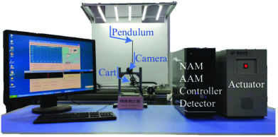
Figure 3: Experimental platform of NIPVSS. NAM: Nominal auxiliary model. AAM: Adaptive auxiliary model.

To validate the proposed MAPDAs, we consider the scenario when TPDAs [Jeon & Eun, 2019], MAPDAs, DFLCAs [Li & Yang, 2018], and TLCAs [Li et al., 2019] are embedded in a networked inverted pendulum visual servo system (NIPVSS) [Du et al., 2020] in Fig. 3.

4.1 Parameters of NIPVSS

The state of NIPVSS is set as $x(t)=[\alpha(t),\theta(t),\dot{\alpha}(t),\dot{\theta}(t)]$, where $\alpha(t)$ is the cart position, $\theta(t)$ is the pendulum angle, $\dot{\alpha}(t)$ and $\dot{\theta}(t)$ are the cart and angular velocity, respectively. The acceleration-as-control-input nonlinear differential equation of the inverted pendulum is

$$lmu\cos\theta+lmg\sin\theta=J\ddot{\theta},$$ (16)

where $l$ is the length from the pivot to the center of the pendulum, $m$ is the mass of the pendulum, $g$ is the acceleration of the gravity, $J$ is the moment of the inertia about the pivot of the pendulum, the values of $l$, $m$, $g$, $J$ can be found in [Du et al., 2020], and $u=\ddot{\alpha}$ is the control input. By linearizing (16) in $\left|{\theta}\right|\leqslant 0.2rad$ (i.e., $\cos\theta\approx 1$ and $\sin\theta\approx\theta$ in $\left|{\theta}\right|\leqslant 0.2rad$), the nominal model $A_{n}$ and $B_{n}$ of (16) is given by

$${A_{n}}=\left[{\begin{array}[]{*{20}{c}}0&0&1&0\\ 0&0&0&1\\ 0&0&0&0\\ 0&29.4311&0&0\end{array}}\right],{B_{n}}=\left[{\begin{array}[]{*{20}{c}}0\\ 0\\ 1\\ 3.0001\end{array}}\right].$$

Based on $A_{n}$, $B_{n}$ and using $H_{\infty}$ control [Du et al., 2020], the controller is designed as

$$K=K_{n}=[3.7569,-29.6225,4.0648,-5.4563].$$

The controlled outputs are $\alpha(t)$ and $\theta(t)$. The admissible limits are $\left|\alpha(t)\right|<0.3m$ and $\left|\theta(t)\right|<0.8rad$.

4.2 Threshold of the Detector

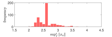
Figure 4: The frequency of different ${{{\sup}^{e}_{f}}\left\|{{x_{a}}}\right\|}$ from all 500 experiments.

To properly set the threshold $\epsilon$ of the detector, in terms of statistical analysis method [Heydt & Graf, 2010], 500 experiments of attack-free NIPVSS are operated (see Fig. A.3 and Table A.2 in Section 4.1 of the supplementary materials [Du et al., 2022]). The frequency of different ${{{\sup}^{e}_{f}}\left\|{{x_{a}}}\right\|}$ (i.e., the upper bound of attack-free $\left\|x_{a}(t)\right\|$) are shown in Fig. 4. It can be seen from Fig. A.3, Table A.2 and Fig. 4 that after the state of NIPVSS is stable, the threshold can be set as $\epsilon=3.1$ based on the 3$\sigma$ principle.

4.3 Performance of TPDAs and MAPDAs

For comparison, we construct two types of attacks with the values of $A_{n}$, $B_{n}$ and $K_{n}$. One is TPDAs [Jeon & Eun, 2019] with $\mathcal{A}_{c,t}(A_{n})$ (10) when $t\geqslant 0s$ (i.e., $k\geqslant 0$). Another is the proposed MAPDAs with ${\mathcal{A}_{a,t}}({A_{n}},\Phi_{n},x_{a})$ (15) when $t\geqslant 0s$ (i.e., $k\geqslant 0$), and their parameters are set as $Q=I$ and $Z=10000I$ in (15), and $P$ is calculated by using (15) as

$$P=\left[{\begin{array}[]{*{20}{c}}{1.7760}&{-2.0855}&{0.8362}&{-0.3231}\\ &{10.6948}&{-2.9413}&{1.4742}\\ &*&{1.0652}&{-0.4646}\\ &*&*&{0.2755}\end{array}}\right].$$

The initial condition is set to $x_{\rm nam}(0)=0.0001\textbf{1}$ in (10), and $x_{\rm aam}(0)=0.0001\textbf{1}$, $F_{a}(0)=I$ in (15). According to the condition of Theorem 2, it is verified in Section 4.2.1 of the supplementary materials [Du et al., 2022] that $x_{\rm nam}(0)=0.0001\textbf{1}$ does not satisfy the item (i) or (ii) of Lemma A.2 in Section 2.5 of the supplementary materials [Du et al., 2022]. Therefore, it satisfies the initial condition of Theorem 2.

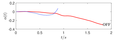
(a) $\alpha(t)$

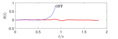
(b) $\theta(t)$

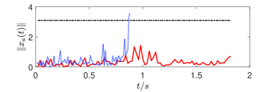
(c) $\left\|{x_{a}}(t)\right\|$

Figure 5: Controlled output and detection results of NIPVSS under TPDAs [Jeon & Eun, 2019] with $\mathcal{A}_{c,t}(A_{n})$ (10) or the proposed MAPDAs with ${\mathcal{A}_{a,t}}({A_{n}},\Phi_{n},x_{a})$ (15) of $Q=I$ and $Z=10000I$. Blue line: Under TPDAs with $\mathcal{A}_{c,t}(A_{n})$ (10). Red Line: Under MAPDAs with ${\mathcal{A}_{a,t}}({A_{n}},\Phi_{n},x_{a})$ (15). Black line in (c): The detection threshold $\epsilon=3.1$.

The experiments are operated using the above set parameters, and the experimental results of NIPVSS under TPDAs with $\mathcal{A}_{c,t}(A_{n})$ (10) and the proposed MAPDAs with ${\mathcal{A}_{a,t}}({A_{n}},\Phi_{n},x_{a})$ (15) are shown in Fig. 5. When there exists model mismatch, we observe that: (1) TPDAs with $\mathcal{A}_{c,t}(A_{n})$ (10) drive the pendulum angle of NIPVSS to cross the maximum allowable angle 0.8 rad shown by the blue line in Fig. 5(b), while the detector succeeds to detect them shown by the blue line in Fig. 5(c), and (2) MAPDAs with ${\mathcal{A}_{a,t}}({A_{n}},\Phi_{n},x_{a})$ (15) cannot be detected shown by the red line in Fig. 5(c) before driving the cart position to cross the allowable limit -0.3 m shown by red line in Fig. 5(a). It confirms that the proposed MAPDAs are not detectable before achieving successful destructiveness.

The above has presented rather good results for the proper parameters $Q$ and $Z$, however if the improper parameters $Q$ and $Z$ are chosen, it will produce less satisfactory experimental results of Figs. A.4 and A.5 in Section 4.2.2 of the supplementary materials [Du et al., 2022].

4.4 Performance of MAPDAs, DFLCAs and TLCAs

For further comparison with the existing methods, three types of attacks are constructed: DFLCAs [Li & Yang, 2018] using both the measurements and control input, TLCAs [Li et al., 2019] using both the measurements and control input (or using only the measurements) and the proposed MAPDAs using only the measurements.

The experimental results of NIPVSS under DFLCAs, TLCAs and MAPDAs with ${\mathcal{A}_{a,t}}({A_{n}},\Phi_{n},x_{a})$ (15) are shown in Fig. 6. When there exists model mismatch, we observe that: (1) DFLCAs drive the pendulum angle and cart position of NIPVSS to cross the allowable limit -0.8 rad and -0.3 m shown by the purple lines in Fig. 6(a) and (b) respectively, while the detector succeeds to detect them shown by the purple line in Fig. 6(c); (2) TLCAs drive the pendulum angle and cart position of NIPVSS to cross the allowable limit -0.8 rad and -0.3 m shown by the green lines in Fig. 6(a) and (b) respectively, while the detector fails to detect them shown by the green line in Fig. 6(c); it can be also seen from the blue line in Fig. 6(c) that once TLCAs do not use control input (i.e., cannot construct the covert agent), they will be detected by the detector; (3) MAPDAs with ${\mathcal{A}_{a,t}}({A_{n}},\Phi_{n},x_{a})$ (15) drive the cart position of NIPVSS to cross the allowable limit -0.3 m shown by the red line in Fig. 6(a), while the detector fails to detect them shown by the red line in Fig. 6(c). Therefore, compared with DFLCAs and TLCAs, the proposed MAPDAs method using only the measurements can bypass the detector, i.e., achieve successfully stealthy attack.

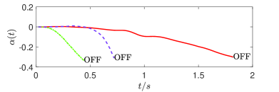
(a) $\alpha(t)$

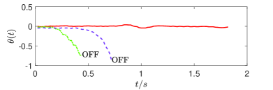
(b) $\theta(t)$

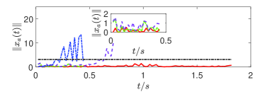
(c) $\left\|{x_{a}}(t)\right\|$

Figure 6: Controlled output and detection results of NIPVSS under DFLCAs [Li & Yang, 2018], TLCAs [Li et al., 2019] and the proposed MAPDAs with ${\mathcal{A}_{a,t}}({A_{n}},\Phi_{n},x_{a})$ (15). Purple line: Under DFLCAs. Green line: Under TLCAs. Blue line in (c): Detection result of TLCAs without using control input. Red Line: Under MAPDAs with ${\mathcal{A}_{a,t}}({A_{n}},\Phi_{n},x_{a})$ (15). Black line in (c): The detection threshold $\epsilon=3.1$.

5 Conclusion

We have shown in this paper that stealthy attacks on vulnerable-sensor-network-only NCSs are possible, particularly when the measurements and adaptive control methods are employed. As a prototype, a stealthy MAPDAs method has been designed by using the measurements and adaptive control methods, and its promising performance on stealthiness and destructiveness are analysed by using convergence of measurements. In the future, the current work can be further extended to quasi-ideal attacks.

The work was supported in part by the National Science Foundation of China under Grant Nos. 92067106, 61773253, 61803252, and 61833011, 111 Project under Grant No. D18003, and Project of Science and Technology Commission of Shanghai Municipality under Grant Nos. 20JC1414000, 19500712300, 19510750300, 21190780300.

References

- [Bjorck, 2015] Bjorck, A. (2015). Numerical Methods in Matrix Computations. Springer, Cham.
- [Du et al., 2022] Du, D., Zhang, C., Peng C., Fei, M., & H. Zhou. (2022). Stealthy measurement-aided pole-dynamics attacks with nominal models. arXiv preprint arXiv: 2210.14403.
- [Du et al., 2020] Du, D., Zhang, C., Song, Y., Zhou, H., Li, X., Fei, M., & Li W. (2020). Real-time control of networked inverted pendulum visual servo systems. IEEE Transactions on Cybernetics, 50(12), 5113–5126.
- [Endrejat & Pillay, 2011] Endrejat, F., & Pillay, P. (2011). Ride-through of medium voltage synchronous machine centrifugal compressor drives. IEEE Transactions on Industry Applications, 47(4), 1567–1577.
- [Heydt & Graf, 2010] Heydt, G. T., & Graf, T. J. (2010). Distribution system reliability evaluation using enhanced samples in a Monte Carlo approach. IEEE Transactions on Power Systems, 25(4), 2006–2008.
- [Guo et al., 2017] Guo, Z., Shi, D., Johansson, K. H., & Shi, L. (2017). Optimal linear cyber-attack on remote state estimation. IEEE Transactions on Control of Network Systems, 4(1), 4–13.
- [Hespanha, 2006] Hespanha, J. P. (2006). Linear Systems Theory. John Wiley & Sons, Ltd.
- [Jeon & Eun, 2019] Jeon, H., & Eun, Y. (2019). A stealthy sensor attack for uncertain cyber-physical systems. IEEE Internet of Things Journal, 6(4), 6345–6352.
- [Kersting & Buss, 2017] Kersting, S., & Buss, M. (2017). Direct and indirect model reference adaptive control for multivariable piecewise affine systems. IEEE Transactions on Automatic Control, 62(11), 5634–5649.
- [Kim et al., 2021] Kim, S., Eun, Y., & Park, K.-J. (2021). Stealthy sensor attack detection and real-time performance recovery for resilient CPS. IEEE Transactions on Industrial Informatics, 17(11), 7412–7422.
- [Kung et al., 2017] Kung, E., Dey, S., & Shi, L. (2017). The performance and limitations of - stealthy attacks on higher order systems. IEEE Transactions on Automatic Control, 62(2), 941-947.
- [Li et al., 2019] Li, W., Xie, L., & Wang, Z. (2019). Two-loop covert attacks against constant value control of industrial control systems. IEEE Transactions on Industrial Informatics, 15(2), 663–676.
- [Li & Yang, 2018] Li, Z., & Yang, G.-H. (2018). A data-driven covert attack strategy in the closed-loop cyber-physical systems. Journal of the Franklin Institute, 355(14), 6454–6468.
- [Ling & Kravaris, 2019] Ling, C., & Kravaris, C. (2019). Multirate sampled-data observer design based on a continuous-time design. IEEE Transactions on Automatic Control, 64(12), 5265–5272.
- [Liu et al., 2017] Liu, C., Wu, J., Long, C., & Wang, Y. (2017). Dynamic state recovery for cyber-physical systems under switching location attacks. IEEE Transactions on Control of Network Systems, 4(1), 14–22.
- [Lyu et al., 2018] Lyu, L., Chen, C., Zhu, S., Cheng, N., Yang, B., & Guan, X. (2018). Control performance aware cooperative transmission in multiloop wireless control systems for industrial IoT applications. IEEE Internet of Things Journal, 5(5), 3954–3966.