Brief introduction to the nonlinear stability of Kerr

Abstract

This a brief introduction to the sequence of works [63], [39], [61], [62] and [81] which establish the nonlinear stability of Kerr black holes with small angular momentum. We are delighted to dedicate this article to Demetrios Christodoulou for whom we both have great admiration. The first author would also like to thank Demetrios for the magic moments of friendship, discussions and collaboration he enjoyed together with him.

1 Kerr stability conjecture

1.1 Kerr spacetime

Let $({\mathcal{K}}(a,m),{\bf g}_{a,m})$ denote the family of Kerr spacetimes depending on the parameters $m$ (mass) and $a$ (with $J=am$ angular momentum). In Boyer-Lindquist coordinates the Kerr metric is given by

$${\bf g}_{a,m}=-\frac{q^{2}\Delta}{\Sigma^{2}}(dt)^{2}+\frac{\Sigma^{2}(\sin\theta)^{2}}{|q|^{2}}\left(d\phi-\frac{2amr}{\Sigma^{2}}dt\right)^{2}+\frac{|q|^{2}}{\Delta}(dr)^{2}+|q|^{2}(d\theta)^{2},$$ (1.1)

where

$$\begin{cases}&\Delta=r^{2}+a^{2}-2mr,\qquad q=r+ia\cos\theta,\\ &\Sigma^{2}=(r^{2}+a^{2})|q|^{2}+2mra^{2}(\sin\theta)^{2}=(r^{2}+a^{2})^{2}-a^{2}(\sin\theta)^{2}\Delta.\end{cases}$$ (1.2)

The asymptotically flat metrics ${\bf g}_{a,m}$ verify the Einstein vacuum equations

$$\mbox{Ric}({\bf g})=0,$$ (1.3)

are stationary and axially symmetric, possess well-defined event horizons $r=r_{+}$ (the largest root of $\Delta(r)=0$), domain of outer communication $r>r_{+}$ and smooth future null infinity ${\mathcal{I}}^{+}$ where $r=+\infty$. The metric can be extended smoothly inside the black hole region, see Figure 1. The boundary $r=r_{-}$ (the smallest root of $\Delta(r)=0$) inside the black hole region is a Cauchy horizon across which predictability fails.

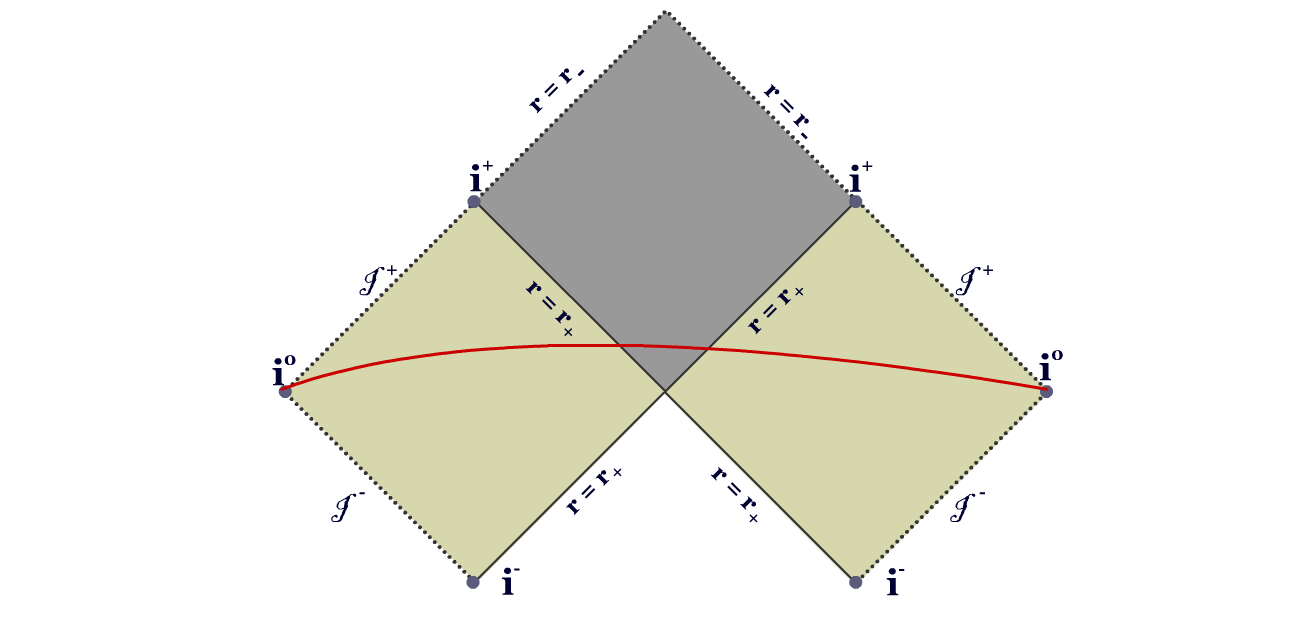
Figure 1: Penrose diagram of Kerr for $0<|a|<m$. The surface $r=r_{+}$, the larger root of $\Delta=0$, is the event horizon of the black hole, $r>r_{+}$ the domain of outer communication, ${\mathcal{I}}^{+}$ is the future null infinity, corresponding to $r=+\infty$.

Here are some of the most important properties of ${\mathcal{K}}(a,m)$:

• ${\mathcal{K}}(a,m)$ possesses a canonical family of null pairs, called principal null pairs, of the form $(\lambda e_{4},\lambda^{-1}e_{3})$, with $\lambda>0$ an arbitrary scalar function, and

  $$\begin{split}e_{4}&=\frac{r^{2}+a^{2}}{|q|^{2}}{\partial}_{t}+\frac{\Delta}{|q|^{2}}{\partial}_{r}+\frac{a}{|q|^{2}}{\partial}_{\phi},\qquad e_{3}=\frac{r^{2}+a^{2}}{\Delta}{\partial}_{t}-{\partial}_{r}+\frac{a}{\Delta}{\partial}_{\phi}.\end{split}$$ (1.4)

• The horizontal structure, perpendicular to $e_{3},e_{4}$, denoted ${\mathcal{H}}$, is spanned by the vectors

  $$e_{1}=\frac{1}{|q|}{\partial}_{\theta},\qquad e_{2}=\frac{a\sin\theta}{|q|}{\partial}_{t}+\frac{1}{|q|\sin\theta}{\partial}_{\phi}.$$ (1.5)

  The distribution generated by ${\mathcal{H}}$ is non-integrable for $a\neq 0$.

• The horizontal structure $(e_{3},e_{4},{\mathcal{H}})$ has the remarkable property that all components of the Riemann curvature tensor ${\bf R}$, decomposed relative to them, vanish with the exception of those which can be deduced from ${\bf R}(e_{a},e_{3},e_{b},e_{4}).$

• ${\mathcal{K}}(a,m)$ possesses the Killing vectorfields ${\bf T},{\bf Z}$ which, in BL coordinates, are given by ${\bf T}={\partial}_{t},{\bf Z}={\partial}_{\phi}$.

• In addition to the symmetries generated by ${\bf T},{\bf Z}$, ${\mathcal{K}}(a,m)$ possesses also a non-trivial Killing tensor, i.e. a symmetric 2-tensor ${\bf C}_{{\alpha}{\beta}}$ verifying the property ${\bf D}_{(\gamma}{\bf C}_{{\alpha}{\beta})}=0$. The tensor carries the name of its discoverer B. Carter, see [15], who made use of it to show that the geodesic flow in Kerr is integrable. Its presence, in addition to ${\bf T}$ and ${\bf Z}$, as a higher order symmetry, is at the heart of what Chandrasekhar, see [17], called the most striking feature of Kerr, “the separability of all the standard equations of mathematical physics in Kerr geometry”.

• The Carter tensor can be used to define the Carter operator

  $${\mathcal{C}}={\bf D}_{\alpha}({\bf C}^{{\alpha}{\beta}}{\bf D}_{\beta}),$$ (1.6)

  a second order operator which commutes with $\square_{a,m}$. This property plays a crucial role in the proof of our stability result, Theorem 1.1, more precisely in Part II of [39].

1.2 Kerr stability conjecture

The discovery of black holes, first as explicit solutions of EVE and later as possible explanations of astrophysical phenomena, has not only revolutionized our understanding of the universe, it also gave mathematicians a monumental task: to test the physical reality of these solutions. This may seem nonsensical since physics tests the reality of its objects by experiments and observations and, as such, needs mathematics to formulate the theory and make quantitative predictions, not to test it. The problem, in this case, is that black holes are by definition non-observable and thus no direct experiments are possible. Astrophysicists ascertain the presence of such objects through indirect observations and numerical experiments, but both are limited in scope to the range of possible observations or the specific initial conditions in which numerical simulations are conducted. One can rigorously check that the Kerr solutions have vanishing Ricci curvature, that is, their mathematical reality is undeniable. But to be real in a physical sense, they have to satisfy certain properties which, as it turns out, can be neatly formulated in unambiguous mathematical language. Chief among them is the problem of stability, that is, to show that if the precise initial data corresponding to Kerr are perturbed a bit, the basic features of the corresponding solutions do not change much.

Conjecture (Stability of Kerr conjecture).  Vacuum, asymptotically flat, initial data sets, sufficiently close to $Kerr(a,m)$, $|a|/m<1$, initial data, have maximal developments with complete future null infinity and with domain of outer communication which approaches (globally) a nearby Kerr solution.

1.3 Resolution of the conjecture for slowly rotating black holes

1.3.1 Statement of the main result

The goal of this article is to give a short introduction to our recent result in which we settle the conjecture in the case of slowly rotating Kerr black holes.

Theorem 1.1.

The future globally hyperbolic development of a general, asymptotically flat, initial data set, sufficiently close (in a suitable topology) to a $Kerr(a_{0},m_{0})$ initial data set, for sufficiently small $|a_{0}|/m_{0}$, has a complete future null infinity ${\mathcal{I}}^{+}$ and converges in its causal past ${\mathcal{J}}^{-1}({\mathcal{I}}^{+})$ to another nearby Kerr spacetime $Kerr(a_{f},m_{f})$ with parameters $(a_{f},m_{f})$ close to the initial ones $(a_{0},m_{0})$.

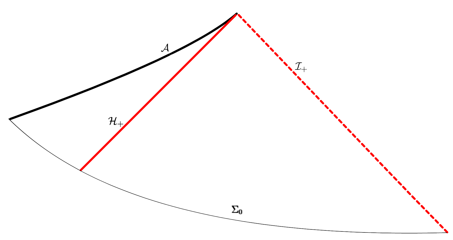
Figure 2: The Penrose diagram of the final space-time in Theorem 1.1 with initial hypersurface $\Sigma_{0}$, future space-like boundary ${\mathcal{A}}$, and ${\mathcal{I}}^{+}$ the complete future null infinity. The hypersurface ${\mathcal{H}}_{+}$ is the future event horizon of the final Kerr.

The precise version of the result, all the main features of the architecture of its proof, as well as detailed proofs for most of the main steps are to be found in [63]. The full proof relies also on our joint work [39] with E. Giorgi, our papers [61], [62] on GCM spheres, and the extension [81] to GCM hypersurfaces by D. Shen.

1.3.2 Brief comments on the proof

We will discuss the main ideas of the proof in more details in section 4. It pays however to give already a graphic sense of the main building blocks of our approach, which we call general covariant modulated(GCM), admissible spacetimes.

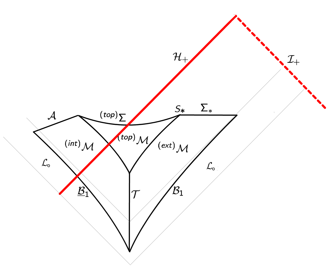
Figure 3: The Penrose diagram of a finite GCM admissible space-time ${\mathcal{M}}={\,{}^{(ext)}\mathcal{M}}\cup{\,{}^{(top)}{\mathcal{M}}}\cup{\,{}^{(int)}{\mathcal{M}}}$. The future boundary $\Sigma_{*}$ initiates at the GCM sphere $S_{*}$. The past boundary of ${\mathcal{M}}$, ${\mathcal{B}}_{1}\cup\underline{\mathcal{{\mathcal{B}}}}_{1}$, is included in the initial layer ${\mathcal{L}}_{0}$, in which the spacetime is assumed given.

The main features of these spacetimes ${\mathcal{M}}={\,{}^{(ext)}\mathcal{M}}\cup{\,{}^{(top)}{\mathcal{M}}}\cup{\,{}^{(int)}{\mathcal{M}}}$ are as follows:

• The capstone of the entire construction is the sphere $S_{*}$, on the future boundary $\Sigma_{*}$ of ${\,{}^{(ext)}\mathcal{M}}$, which verifies a set of specific extrinsic and intrinsic conditions denoted by the acronym GCM.

• The spacelike hypersurface $\Sigma_{*}$, initialized at $S_{*}$, verifies a set of additional GCM conditions.

• Once $\Sigma_{*}$ is specified the whole GCM admissible spacetime ${\mathcal{M}}$ is determined by a more conventional construction, based on geometric transport type equations.

• The construction, which also allows us to specify adapted null frames, is made possible by the covariance properties of the Einstein vacuum equations.

• The past boundary ${\mathcal{B}}_{1}\cup\underline{\mathcal{{\mathcal{B}}}}_{1}$ of ${\mathcal{M}}$, which is itself to be constructed, is included in the initial layer ${\mathcal{L}}_{0}$ in which the spacetime is assumed to be known, i.e. a small vacuum perturbation of a Kerr solution.

The proof of Theorem 1.1 is centered around a limiting argument for a continuous family of such spacetimes ${\mathcal{M}}$ together with a set of bootstrap assumptions (BA) for the connection and curvature coefficients, relative to the adapted frames. Assuming that a given finite, GCM admissible, spacetime ${\mathcal{M}}$ saturates BA we reach a contradiction as follows:

• First improve BA for some of the components of the curvature tensor with respect to the frame. These verify equations (called Teukolsky equations) which decouple, up to terms quadratic in the perturbation, and are treated by wave equations methods.

• Use the information provided by these curvature coefficients together with the gauge choice on ${\mathcal{M}}$, induced by the GCM condition on $\Sigma_{*}$, to improve BA for all other Ricci and curvature components.

• Use these improved estimates to extend ${\mathcal{M}}$ to a strictly larger spacetime ${\mathcal{M}}^{\prime}$ and then construct a new GCM sphere $S_{*}^{\prime}$, a new boundary $\Sigma_{*}^{\prime}$ which initiates on $S_{*}^{\prime}$, and a new GCM admissible spacetime ${\mathcal{M}}^{\prime}$, with $\Sigma_{*}^{\prime}$ as boundary, strictly larger than ${\mathcal{M}}$.

Remark 1.2.

The critical new feature of this argument is the fact that the new GCM sphere $S_{*}^{\prime}$ has to be constructed as a co-dimension 2 sphere in ${\mathcal{M}}^{\prime}$ with no reference to the initial conditions. This construction appears first in [60] in a polarized situation. The general construction appears in the GCM papers [61], [62]. The construction of $\Sigma_{*}^{\prime}$ from $S_{*}^{\prime}$ appears first in [60] in the polarized case. The general construction used in our work is due to D. Shen [81].

2 Linear and nonlinear stability

2.1 Notions of nonlinear stability

Consider a stationary solution $\phi_{0}$ of a nonlinear evolution equation

$${\mathcal{N}}[\phi]=0.$$ (2.1)

There are two distinct notions of stability, orbital stability, according to which small perturbations of $\phi_{0}$ lead to solutions $\phi$ which remain close for all time, and asymptotic stability (AS) according to which the perturbed solutions converge as $t\to\infty$ to $\phi_{0}$. In the case where $\phi_{0}$ is non trivial, there is a third notion, which we call asymptotic orbital stability (AOS), to describe the fact that the perturbed solutions may converge to a different stationary solution. This happens if $\phi_{0}$ belongs to a multi parameter smooth family of stationary solutions, or by applying a gauge transform to $\phi_{0}$ which keeps the equation invariant.

For quasilinear equations, such as EVE, a proof of stability means necessarily AS or AOS stability. Both require a detailed understanding of the decay properties of the linearized equation, i.e.

$${\mathcal{L}}[\phi_{0}]\psi=0,$$ (2.2)

with ${\mathcal{L}}[\phi_{0}]$ the Fréchet derivative ${\mathcal{N}}^{\prime}[\phi_{0}]$. This is, essentially, a linear hyperbolic system with variable coefficients which, typically, presents instabilities.

In the exceptional situation, when stability can ultimately be established, one can tie all the instability modes to the following properties of the nonlinear equation:

1. If $\phi_{\lambda}$ is a family of stationary solutions, near $\phi_{0}$, verifying ${\mathcal{N}}[\phi_{\lambda}]=0$. Then $\psi_{0}=(\frac{d}{d\lambda}\phi_{\lambda})_{\lambda=0}$ verifies ${\mathcal{N}}^{\prime}[\phi_{0}]\psi_{0}=0$, i.e. $\psi_{0}$ is a nontrivial, stationary, bound state of the linearized equations (2.2).

2. If $\Phi_{\lambda}$ is a smooth family of diffeomorphisms of the background manifold, $\Phi_{0}=I$, such that ${\mathcal{N}}[\Phi^{*}_{\lambda}(\phi_{0})]=0$. Then $\Psi_{0}=\big{(}\frac{d}{d\lambda}\Phi^{*}_{\lambda}(\phi_{0})\big{)}_{\lambda=0}$ verifies ${\mathcal{N}}^{\prime}[\phi_{0}]\Psi_{0}=0$, i.e. $\Psi_{0}$ is also a stationary bound state of the linearized equation (2.2).

These linear instabilities are responsible for the fact that a small perturbation of the fixed stationary solution $\phi_{0}$ may not converge to $\phi_{0}$ but to another nearby stationary solution.

To prove the asymptotic convergence of $\phi$ to a final state $\phi_{f}$, different form $\phi_{0}$, we need to establish sufficiently strong rates of decay for $\phi-\phi_{f}$. Rates of decay however are strongly coordinate dependent, i.e. dependent on the choice of the diffeomorphism (or gauge) $\Phi$ in which decay is measured. Thus, to prove a nonlinear stability, result we need to know both the final state $\phi_{f}$ and the coordinate system $\Phi_{f}$ in which sufficient decay, and thus convergence to $\phi_{f}$, can be established. The difficulty here is that neither $\phi_{f}$ nor $\Phi_{f}$ can be determined a-priori (from the initial perturbation), they have to emerge dynamically in the process of convergence. Moreover, in all examples involving nonlinear wave equations in $1+3$ dimensions, the nonlinear terms have to also cooperate, that is an appropriate version of the so called null condition has to be verified.

To summarize, given a nonlinear system ${\mathcal{N}}[\phi]=0$ which possesses both a smooth family of stationary solutions $\phi_{\lambda}$ and a smooth family of invariant diffeomorphisms a proof of the nonlinear stability of $\phi_{0}$ requires the following ingredients:

• The only non-decaying modes of the linearized equation ${\mathcal{L}}(\phi_{0})\psi=0$ are those due to the items M1–M2 above. In particular there are no exponentially growing modes.

• A dynamical construction of both the final state $\phi_{f}$ and the final gauge $\Phi_{f}$ in which convergence to the final state takes place.

• The nonlinear terms in the equation

  $${\mathcal{L}}[\phi_{f}]\psi=N(\psi)$$

  obtained by expanding the equation ${\mathcal{N}}[\phi]$ near $\phi_{f}$, in the gauge given by the diffeomorphism $\Phi_{f}$, has to verify an appropriate version of the null condition.

2.2 The case of the Kerr family

The issue of the stability of the Kerr family has been at the center of attention of GR physics and mathematical relativity for more than half a century, ever since their discovery by Kerr in [51]. In this case we have to deal not only with a $2$-parameter family of solutions, corresponding to the parameters $(a,m)$, but also with the entire group of diffeomorphisms of ${\mathcal{M}}$. In what follows we try to discuss the main difficulties of the problem. In doing that it helps to compare these to those arising in the simplest case when $a=m=0$, i.e. stability of Minkowski.

2.3 Stability of Minkowski space

Until very recently the only space-time for which full nonlinear stability had been established was the Minkowski space, see [25]. The proof is based on some important PDE advances of late last century:

1. Robust approach, based on the vectorfield method, to derive quantitative decay based on generalized energy estimates and commutation with (approximate) Killing and conformal Killing vectorfields.

2. The null condition identifying the deep mechanism for nonlinear stability, i.e. the specific structure of the nonlinear terms which enables stability despite the low decay of the perturbations.

3. Elaborate bootstrap argument according to which one makes educated assumptions about the behavior of solutions to nonlinear wave equations and then proceeds, by a long sequence of a-priori estimates, to show that they are in fact satisfied. This amounts to a conceptual linearization, i.e. a method by which the equations become, essentially, linear without actually linearizing them.

The main innovation in the proof in [25] is the choice of an appropriate gauge condition, readjusted dynamically through the convergence process, by a continuity argument, which allows one to separate the curvature estimates, treated by hyperbolic methods, from the estimates for the connection coefficients. The key point is that these latter verify transport or elliptic equations in which the curvature terms appear as sources. Thus both the curvature components and connection coefficients can be controlled by a bootstrap argument. The gauge condition is based on the constructive choice of a maximal time function $t$ and two outgoing optical functions ${}^{(int)}u$ and ${}^{(ext)}u$ covering the interior and exterior parts of the spacetime.

Another novelty of [25] was the reliance on null frames adapted to the $S$-foliations induced by the level surfaces of $t$ and $u$. These define integrable horizontal structures (in the language of part I of [39]), by contrast with the non-integrable ones used in the proof of Theorem 1.1 and discussed in section 4.3.2. The functions $t,u$ and this integrable horizontal structure can be used to define approximate Killing vectorfields used in estimating the curvature.

2.4 Main difficulties

There are a few major obstacles in passing from the stability of Minkowski to that of Kerr:

1. The first one was already discussed in section 2.1 in the general context of the stability of a stationary solution $\phi_{0}$. In the case when $\phi_{0}$ is trivial there are no nontrivial bound states for the linearized problem and thus we expect that the final state does actually coincide with $\phi_{0}$. This is precisely the case for the special member of the Kerr family $a=m=0$, i.e. the Minkowski space $({\mathbb{R}}^{1+3},m)$. On the other hand, in perturbations of Kerr, general covariance affects the entire construction of the spacetime. In the proof of Theorem 1.1 the crucial concept of a GCM admissible spacetime is meant to deal with both finding the final parameters and the gauge in which convergence to the final state takes place.

2. A fundamental insight in the stability of the Minkowski space was that the Bianchi identities decouple at first order from the null structure equations which allows one to control curvature first, as a Maxwell type system (see [24]), and then proceed with the rest of the solution. This cannot work for perturbations of Kerr due to the fact that some of the null components of the curvature tensor are non-trivial in Kerr.

3. Even if one succeeds in tackling the above mentioned issues, there are still major obstacles in understanding the decay properties of the solution. Indeed, when one considers the simplest, relevant, linear equation on a fixed Kerr background, i.e. the scalar wave equation $\square_{a,m}\psi=0$, one encounters serious difficulties to prove decay. Below is a very short description of these:

   • The problem of trapped null geodesics. This concerns the existence of null geodesics neither crossing the event horizon nor escaping to null infinity, along which solutions can concentrate for arbitrary long times. This leads to degenerate energy-Morawetz estimates which require a very delicate analysis.

   • The trapping properties of the horizon. The horizon itself is ruled by null geodesics, which do not communicate with null infinity and can thus concentrate energy. This problem was solved by understanding the so called red-shift effect associated to the event horizon, which counteracts this type of trapping.

   • The problem of superradiance. This is the failure of the stationary Killing field ${\bf T}=\partial_{t}$ to be everywhere timelike in the domain of outer communication, and thus, of the associated conserved energy to be positive. Note that this problem is absent in Schwarzschild and, in general, for axially symmetric solutions of EVE. In both cases however there still is a degeneracy along the horizon.

   • Superposition problem. This is the problem of combining the estimates in the near region, close to the horizon, (including the ergoregion and trapping) with estimates in the asymptotic region, where the spacetime is close to Minkowski.

4. Though, as seen above, the analysis of the scalar wave equation in Kerr presents formidable difficulties, it is itself just a vastly simplified model problem. A more realistic equation is the so called spin 2 wave equation, or Teukolsky equation, which presents many new challenges.

5. The full linearized system, whatever its formulation, presents many additional difficulties due to its complex tensorial structure and the huge gauge covariance of the equations. The crucial breakthrough in this regard is the observation, due to Teukolsky [89], that the extreme components of the linearized curvature tensor are both gauge invariant (see below in section 2.5) and verify decoupled spin 2 equations, that is the Teukolsky equations mentioned above.

6. A crucial simplification of the linear theory, by comparison to the full nonlinear case, is that one can separate the treatment of the gauge invariant extreme curvature components form all the other gauge invariant quantities. In the nonlinear case this separation is no longer true, all quantities need to be treated simultaneously. Moreover, methods based on separation of variables, developed to treat scalar and and spin 2 wave equations in Kerr, are incompatible with the nonlinear setting which requires, instead, robust methods to derive decay.

2.5 Linear stability

Linear stability for the vacuum equations is formulated in the following way. Given the Einstein tensor ${\bf G}_{{\alpha}{\beta}}={\bf R}_{{\alpha}{\beta}}-\frac{1}{2}{\bf R}{\bf g}_{{\alpha}{\beta}}$ and a stationary solution ${\bf g}_{0}$, i.e. a fixed Kerr metric, one has to solve the system of equations

$${\bf G}^{\prime}({\bf g}_{0})\,\delta{\bf g}=0.$$ (2.3)

The covariant properties of the Einstein equations, i.e. the equivalence between a solution ${\bf g}$ and $\Phi^{*}({\bf g})$, leads us to identify $\delta{\bf g}$ with $\delta{\bf g}+{\mathcal{L}}_{X}({\bf g}_{0})$ for arbitrary vectorfields $X$ in ${\mathcal{M}}$, i.e.

$$\delta{\bf g}\equiv\delta{\bf g}+{\mathcal{L}}_{X}({\bf g}_{0}).$$ (2.4)

We can now attempt to formulate a version of linear stability for (2.3), loosely related to the nonlinear stability of Kerr conjecture, as follows.

Definition 2.1.

By linear stability of the Kerr metric ${\bf g}_{0}$ we understand a result which achieves the following:

Given an appropriate initial data for a perturbation $\delta{\bf g}$, find a vectorfield $X$ such that, after projecting away the bound states generated by the parameters $a,m$ according to M1–M2 in section 2.1, all solutions of the form $\delta{\bf g}+{\mathcal{L}}_{X}{\bf g}_{0}$ to (2.3), decay, relative to an appropriate null frame of ${\mathcal{K}}(a_{0},m_{0})$, sufficiently fast in time.

Remark 2.2.

The definition above is necessarily vague. What is the meaning of sufficiently fast? In fact various components of the metric $\delta{\bf g}$, relative to the canonical null frame of ${\mathcal{K}}(a,m)$, are expected to decay at different polynomial rates, some of which are not even integrable. Unlike in the nonlinear context, where one needs precise rates of decay for components of the curvature tensor and Ricci coefficients, as well as their derivatives, to be able to control the nonlinear terms, in linear theory any type of nontrivial control of solutions may be regarded as satisfactory. Thus linear stability, as formulated above, can only be regarded as a vastly simplified model problem. Nevertheless the study of linear stability of the Kerr family has turned out to be useful in various ways, as we shall see below.

Historically, the following versions of linear stability have been considered.

• Metric Perturbations. At the level of the metric itself, i.e. as above in (2.3).

• Curvature Perturbations. Via the Newman-Penrose (NP) formalism, based on null frames.

The strategy followed in both cases is:

• Find components of the metric (in case (a)) or curvature tensor (in case (b)), invariant with respect to linearized gauge transformations 2.4 which verify simple, decoupled, wave equations. The main insight of this type was the discovery, by Teukolsky [89], in the context of (b) above, that the extreme components of the linearized curvature tensor verify both these properties.

• Analyze these components by showing one of the following:

  • There are no exponentially growing modes. This is known as mode stability.

  • Boundedness for all time.

  • Decay (sufficiently fast) in time.

• Find a linearized gauge condition, i.e. a vectorfield $X$, such that all remaining (gauge dependent) components (at the metric or curvature level) inherit the property mentioned above: no exponentially growing modes, boundedness, or decay in time. In the physics literature this is known as the problem of reconstruction.

2.5.1 Mode stability

All results on the linear stability of Kerr in the physics literature during the 10-15 years after Roy Kerr’s 1963 discovery, often called the “Golden Age of Black Hole Physics”, are based on mode decompositions. One makes use of the separability of the linearized equations, more precisely the Teukolsky equations, on a fixed Kerr background, to derive simple ODEs for the corresponding modes. One can then show, by ingenious methods, that these modes cannot exhibit exponential growth. The most complete result of this type is due to Bernard Whiting [93].

The obvious limitation of these results are as follows:

• They are far from even establishing the boundedness of general solutions to the Teukolsky equations, let alone to establish quantitative decay for the general solutions.

• Results based on mode decompositions depend strongly on the specific symmetries of Kerr which cannot be adapted to perturbations of Kerr.

Robust methods to deal with both issues have been developed in the mathematical community, based on the vectorfield method which we discuss below.

2.5.2 Classical vectorfield method

The vectorfield method, as an analytic tool to derive decay, was first developed in connection with the wave equation in Minkowski space. As well known, solutions of the wave equation $\square\psi=0$ in the Minkowski space ${\mathbb{R}}^{n+1}$ both conserve energy and decay uniformly in time like $t^{-\frac{n-1}{2}}$. While conservation of energy can be established by a simple integration by parts, and is thus robust to perturbations of the Minkowski metric, decay was first derived either using the Kirchhoff formula or by Fourier methods, which are manifestly not robust. An integrated version of local energy decay, based on an inspired integration by parts argument, was first derived by C. Morawetz [74], [75]. The first derivation of decay based on the commutations properties of $\square$ with Killing and conformal Killing vectorfields of Minkowski space together with energy conservation appear in [52] and [55]. The same method also provides precise information about the decay properties of derivatives of solutions with respect to the standard null frame of Minkowski space, an important motivating factor in the discovery of the null condition [53], [22] and [54].

The crucial feature of the methodology initiated by these papers, to which we refer as the classical vectorfield method, is that it can be easily adapted to perturbations of the Minkowski space. As such the method has had numerous applications to nonlinear wave equations and played an important role in the proof of the nonlinear stability of Minkowski space, as discussed in section 2.3. It has also been applied to later versions of the stability of Minkowski in [57]-[58], [67], [9], [66], [44], [43], [40], and extensions of it to Einstein equation coupled with various matter fields in [10], [34], [68], [11], [92], [65], [48].

2.5.3 New vectorfield method

To derive decay estimates for solutions of wave equations on a Kerr background one has to substantially refine the classical vectorfield method. The new vectorfield method is an extension of the classical method which compensates for the lack of enough Killing and conformal Killing vectorfields in Kerr by introducing, new, cleverly designed, vectorfields whose deformation tensors have coercive properties in different regions of spacetime, not necessarily causal. The method has emerged in the last 20 years in connection to the study of boundedness and decay for the scalar wave equation in Schwarzschild and Kerr, see section 3.2 for more details.

2.6 Model problems

To solve the stability of Kerr conjecture one has to deal simultaneously with all the difficulties mentioned above. This is, of course, beyond the abilities of mere humans. Instead the problem was tackled in a sequence of steps based on a variety of simplified model problems, in increasing order of difficulty. To start with we can classify model problems based on the following criteria:

1. Whether the result refers to Schwarzschild i.e. $a=0$, slowly rotating Kerr i.e. $|a|\ll m$ or full non-extremal Kerr $|a|<m$.

2. Whether the result refers to linear or nonlinear stability.

3. Whether the result, in linear theory, refers to scalar wave equation, i.e. spin $0$, Teukolsky equation, i.e. spin $2$, or the full linearized system.

4. Whether the stability result, in linear theory, is a mode stability result, a boundedness result or one that establishes quantitative decay.

3 Short survey of model problems

We give below a short outline of the main developments concerning linear and nonlinear model problems for the Kerr stability problem, paying special attention to those which had a measurable influence on our work.

3.1 Mode stability results

These are mode stability results, using the method of separation of variables, obtained in the physics community roughly during the period 1963-1990. They rely on what Chandrasekhar called the most striking feature of Kerr i.e. “the separability of all the standard equations of mathematical physics in Kerr geometry”.

1. Regge-Wheeler (1957). Even before the discovery of the Kerr solution physicists were interested in the mode stability of Schwarzschild space, i.e. ${\mathcal{K}}(0,m)$. The first important result goes back to T. Regge and J.A Wheeler [78], in which they analyzed linear, metric perturbations, of the Schwarzschild metric. They showed that in a suitable gauge, equation (2.3) decouples into even-parity and odd-parity perturbations, corresponding to axial and polar perturbations. The most important discovery in that paper is that of the master Regge-Wheeler equation, a wave equation with a favorable potential, verified by an invariant scalar component $\phi$ of the metric, i.e.

   $$\square_{m}\phi=V\phi,\qquad V=\frac{4}{r^{2}}\left(1-\frac{2m}{r}\right).$$ (3.1)

   where $\square_{m}$ denotes the wave operator of the Schwarzschild metric of mass $m$. The R-W study was completed by Vishveshwara [90] and Zerilli [94]. A gauge-invariant formulation of metric perturbations was then given by Moncrief [73].

2. Teukolsky (1973). The curvature perturbation approach, near Schwarzschild, based on the Newman-Penrose (NP) formalism was first undertaken by Bardeen-Press [8]. This approach was later extended to the Kerr family by Teukolsky [89], see also [77], who made the important discovery that the extreme curvature components, relative to a principal null frame, are gauge invariant and satisfy decoupled, separable, wave equations. The equations, bearing the name of Teukolsky, are roughly of the form

   $$\square_{a,m}\psi={\mathcal{L}}[\psi]$$ (3.2)

   where ${\mathcal{L}}[\psi]$ is a first order linear operator in $\psi$.

3. Chandrasekhar (1975). In [16] Chandrasekhar initiated a transformation theory relating the two approaches. He exhibited a transformation which connects the Teukolsky equations to a Regge-Wheeler type equation. In the particular case of Schwarzschild the transformation takes the Teukolsky equation to the Regge-Wheeler equation in (3.1). The Chandrasekhar transformation was further elucidated and extended by R. Wald [91] and recently by Aksteiner and al [1].

   Though originally it was meant only to unify the Regge-Wheeler approach with that of Teukolsky, the Chandrasekhar transformation, and various extensions of it, turn out to play an important role in the field.

4. Whiting (1989). As mentioned before the full mode stability, i.e. lack of exponentially growing modes, for the Teukolsky equation on Kerr is due to Whiting [93] (see also [83], in the case of the scalar wave equation, and [5] [88] for stronger quantitive versions).

5. Reconstruction. Once we know that the Teukolsky variables, i.e. the extreme components of the curvature tensor verify mode stability, i.e. there are no exponentially growing modes, it still remains to deal with the problem of reconstruction, i.e. to find a gauge relative to which all other components of the curvature and Ricci coefficients enjoy the same property. We refer the reader to Wald [91] and the references within for a treatment of this issue in the physics literature.

3.2 Quantitative decay for the scalar wave equation

As mentioned in section 2.5.1, mode stability is far from establishing even the boundedness of solutions. To achieve that and, more importantly, to derive realistic decay estimates, one needs an entirely different approach based on what we called the “new vectorfield method” in section 2.5.3. The method has emerged in connection to the study of boundedness and decay for the scalar wave equation in ${\mathcal{K}}(a,m)$,

$$\square_{a,m}\phi=0.$$ (3.3)

The starting and most demanding part of the new method, which appeared first in [12], is the derivation of a global, combined, Energy-Morawetz estimate which degenerates in the trapping region. Once an Energy-Morawetz estimate is established one can commute with the Killing vectorfields of the background manifold, and the so called red shift vectorfield introduced in [26], to derive uniform bounds for solutions. The most efficient way to also get decay, and solve the superposition problem (see section 2.4), originating in [27], is based on the presence of family of $r^{p}$-weighted, quasi-conformal vectorfields defined in the non-causal, far $r$ region of spacetime.

The first Energy-Morawetz type results for scalar wave equation (3.3) in Schwarzschild, i.e. $a=0$, are due to Soffer-Blue [12], [13] and Blue-Sterbenz [14], based on a modified version of the classical Morawetz integral energy decay estimate. Further developments appear in the works of Dafermos-Rodnianski, see [26], [27], and Marzuola-Metcalfe-Tataru-Tohaneanu [71]. The vectorfield method can also be extended to derive decay for axially symmetric solutions in Kerr, see [47] and [85], but it is known to fail for general solutions in Kerr, see Alinhac [2].

In the absence of axial symmetry the derivation of an Energy-Morawetz estimate in ${\mathcal{K}}(a,m)$ for $|a/m|\ll 1$ requires a more refined analysis involving both the vectorfield method and either micro-local methods or mode decompositions. The first full quantitative decay result, based on micro-local analysis techniques, is due to Tataru-Tohaneanu [87]. The derivation of such an estimate in the full sub-extremal case $|a|<m$ is even more subtle and was achieved by Dafermos-Rodnianski-Shlapentokh-Rothman [29] by combining the vectorfield method with a full separation of variables approach. A purely physical space proof of the Energy-Morawetz estimate for small $|a/m|$, which avoids both micro-local analysis and mode decompositions, was pioneered by Andersson-Blue in [4]. Their method, which extends the classical vectorfield method to include second order operators (in this case the Carter operator, see section 1.1), has the usual advantages of the classical vectorfield method, i.e it is robust with respect to perturbations. It is for this reasons that we rely on it in the proof of Theorem 1.1, more precisely in part II of [39].

3.3 Linear stability of Schwarzschild

A first quantitative proof of the linear stability of Schwarzschild spacetime was established by Dafermos-Holzegel-Rodnianski (DHR) in [30]. Notable in their analysis is the treatment of the Teukolsky equation in a fixed Schwarzschild background. While the Teukolsky equation is separable, and amenable to mode analysis, it is not variational and thus cannot be treated directly by energy type estimates. As mentioned earlier in section 3.1, Chandrasekhar was able to relate the Teukolsky equation to the Regge-Wheeler (RW) equation, which is both variational and coercive (the potential $V$ has a favorable sign). In [30] the authors rely on a physical space version of the Chandrasekhar transformation. Once decay estimates for the RW equation have been established, based on the technology developed earlier for the scalar wave equation in Schwarzschild, the authors recover the expected boundedness and decay for solutions to the original Teukolsky equation.

The remaining work in [30] is to derive similar control for the other curvature components and the linearized Ricci coefficients associated to the double null foliation. This last step requires carefully chosen gauge conditions, which the authors make within the framework of a double null foliation, initialized both on the initial hypersurface and the background Schwarzschild horizon. This gauge fixing from initial data leads to sub-optimal decay estimates for some of the metric coefficients and is thus inapplicable to the nonlinear case. This deficiency was fixed in the PhD thesis of E. Giorgi, in the context of the linear stability of Reissner-Nordström, see [38], by relying on a linearized version of the GCM construction in [60].

3.4 Linear stability of Kerr for small angular momentum

The first breakthrough result on the linear stability of Kerr, for $|a|/m\ll 1$, is due to Ma [69], see also [31]. Both results are based on a generalization of the Chandrasekhar transformation to Kerr which takes the Teukolsky equations, verified by the extreme curvature components, to generalized versions of the Regge-Wheeler (gRW) equation. Relying on separation of variables and vectorfield techniques, similar to those developed for the scalar wave equation in slowly rotating Kerr, the authors derive Energy-Morawetz and $r^{p}$ estimates for the solutions of the gRW equations. These results were recently partially extended to the full subextremal range in [84].

The first stability results for the full linearized Einstein vacuum equations near ${\mathcal{K}}(a,m)$, for $|a|/m\ll 1$, appeared in [6] and [41]. The first paper, based on the GHP formalism, see [37], builds on the results of [69] while the second paper is based on an adapted version of the metric formalism and builds on the seminal work of the authors on Kerr-de Sitter [42]. Though the ultimate relevance of these papers to nonlinear stability remains open, they are both remarkable results in so far as they deal with difficulties that looked insurmountable even ten years ago.

3.5 Nonlinear model problems

3.5.1 Nonlinear stability of Kerr-de Sitter

There is another important, simplified, nonlinear model problem which has drawn attention in recent years, due mainly to the striking achievement of Hintz and Vasy [42]. This is the problem of stability of Kerr-de Sitter concerning the Einstein vacuum equation with a strictly positive cosmological constant

$${\bf R}_{{\alpha}{\beta}}+\Lambda{\bf g}_{{\alpha}{\beta}}=0,\qquad\Lambda>0.$$ (3.4)

In their work, which relies in part on the important mode stability result of Kodama and Ishibashi [64], Hintz and Vasy were able prove the nonlinear stability of the stationary part of Kerr-de Sitter with small angular momentum, the first nonlinear stability result of any nontrivial stationary solutions for the Einstein equations. It is important to note that, despite the fact that, formally, the Einstein vacuum equation (1.3) is the limit of (3.4) as $\Lambda\to 0$, the global behavior of the corresponding solutions is radically different.

The main simplification in the case of stationary solutions of (3.4) is that the expected decay rates of perturbations near Kerr-de Sitter is exponential, while in the case $\Lambda=0$ the decay is lower degree polynomial, with various components of tensorial quantities decaying at different rates, and the slowest decaying rate being no better than $t^{-1}$. The Hintz-Vasy result was recently revisited in the work of A. Fang [35] [36] where he bridges the gap between the spectral methods of [42] and the vectorfield methods.

3.5.2 Nonlinear stability of Schwarzschild

The first nonlinear stability result of the Schwarzschild space was established in [60]. In its simplest version, the result states the following.

Theorem 3.1 (Klainerman-Szeftel [60]).

The future globally hyperbolic development of an axially symmetric, polarized, asymptotically flat initial data set, sufficiently close (in a specified topology) to a Schwarzschild initial data set of mass $m_{0}>0$, has a complete future null infinity ${\mathcal{I}}^{+}$ and converges in its causal past ${\mathcal{J}}^{-1}({\mathcal{I}}^{+})$ to another nearby Schwarzschild solution of mass $m_{f}$ close to $m_{0}$.

The restriction to axial polarized perturbations is the simplest assumption which insures that the final state is itself Schwarzschild and thus avoids the additional complications of the Kerr stability problem. We refer the reader to the introduction in [60] for a full discussion of the result.

The proof is based on a construction based on GCM admissible spacetimes similar to that briefly discussed in section 1.3 in the context of slowly rotating Kerr. There are however several important simplifications to be noted:

• The assumption of polarization makes the constructions of the GCM spheres $S_{*}$ and spacelike hypersurface $\Sigma_{*}$ significantly simpler, see Chapter 9 in [60], by comparison to the general case treated in [61], [62] and [81].

• The spacetime has only two components ${\mathcal{M}}={\,{}^{(ext)}\mathcal{M}}\cup{\,{}^{(int)}{\mathcal{M}}}$ and the null horizontal structures, defined on each component, are integrable.

• As in the case of the scaler wave equation on Schwarzschild space the main spin-2 Teukolsky wave equations can be treated by a vectorfield approach. This is no longer true in Kerr and even less so in perturbations of Kerr.

Figure 4: The GCM admissible space-time $\mathcal{M}$. By comparison to Figure 3, ${\mathcal{M}}$ does not have ${\,{}^{(top)}{\mathcal{M}}}$, the past boundaries ${\mathcal{C}}_{0}\cup\underline{\mathcal{C}}_{0}$ and future boundary $\underline{\mathcal{C}}\cup\underline{\mathcal{C}}_{*}$ are null and the horizontal structures (induced by geodesic foliations) are integrable. As in Theorem 1.1, the crucial GCM sphere $S_{*}$ is defined and constructed with no reference to the initial data.

Recently Dafermos-Holzegel-Rodnianski-Taylor [32] have extended the result of [60] by properly preparing a co-dimension 3 subset of the initial data such that the final state is still Schwarzschild. Like in [60], the starting point of [32] is to anchor the entire construction on a far away GCM type sphere $S_{*}$, in the sense of [61] [62], with no direct reference to the initial data. It also uses the same definition of the angular momentum as in (7.19) of [62]. Finally, the spacetime in [32] is separated in an exterior region ${\,{}^{(ext)}\mathcal{M}}$ and an interior region ${\,{}^{(int)}{\mathcal{M}}}$, with the ingoing foliation of ${\,{}^{(int)}{\mathcal{M}}}$, initialized based on the information induced by ${\,{}^{(ext)}\mathcal{M}}$, as in [60]. We note, however, that [32] does not use the geodesic foliation of [60], but instead both ${\,{}^{(int)}{\mathcal{M}}}$ and ${\,{}^{(ext)}\mathcal{M}}$ are foliated by double null foliations, and thus, the process of estimating the gauge dependent variables is somewhat different.

4 Main ideas in the proof of Theorem 1.1

4.1 The bootstrap region

As mentioned in section 1.3.2, the proof of Theorem 1.1 is centered around a limiting argument for a family of carefully constructed finite generally covariant modulated (GCM) admissible spacetimes ${\mathcal{M}}={\,{}^{(ext)}\mathcal{M}}\cup{\,{}^{(top)}{\mathcal{M}}}\cup{\,{}^{(int)}{\mathcal{M}}}$. As can be seen in Figure 5 below, the future boundary of the spacetime is given by ${\mathcal{A}}\cup{\,{}^{(top)}\Sigma}\cup\Sigma_{*}$ where $\Sigma_{*}$ is a spacelike, generally covariant modulated (GCM) hypersurface, that is a hypersurface verifying a set of crucial, well-specified, geometric conditions, essential to our proof of convergence to a final state.

Figure 5: The Penrose diagram of a finite GCM admissible space-time ${\mathcal{M}}={\,{}^{(ext)}\mathcal{M}}\cup{\,{}^{(top)}{\mathcal{M}}}\cup{\,{}^{(int)}{\mathcal{M}}}$. The spacetime is prescribed in the initial layer ${\mathcal{L}}_{0}$ and has ${\mathcal{A}}\cup{\,{}^{(top)}\Sigma}\cup\Sigma_{*}$ as future boundary, with $\Sigma_{*}$ a spacelike “generally covariant modulated (GCM)” hypersurface. Its past boundary, ${\mathcal{B}}_{1}\cup\underline{\mathcal{{\mathcal{B}}}}_{1}$, is itself part of the construction. ${\,{}^{(ext)}\mathcal{M}}$ is initialized by the GCM hypersurface $\Sigma_{*}$ while ${\,{}^{(int)}{\mathcal{M}}}$ is initialized on ${\mathcal{T}}$ by the foliation induced by ${\,{}^{(ext)}\mathcal{M}}$. The main inovation is the GCM sphere $S_{*}$, defined and constructed with no reference to the initial data prescribed in the initial data layer ${\mathcal{L}}_{0}$.

The capstone as well as the most original part of the entire construction is the sphere $S_{*}$, the future boundary of $\Sigma_{*}$, which verifies a set of rigid, extrinsic and intrinsic, conditions. Once $\Sigma_{*}$ is specified the whole GCM admissible spacetime ${\mathcal{M}}$ is determined by a more conventional construction, based on geometric transport type equations. More precisely ${\,{}^{(ext)}\mathcal{M}}$ can be determined from $\Sigma_{*}$ by a specified outgoing foliation terminating in the timelike boundary ${\mathcal{T}}$, ${\,{}^{(int)}{\mathcal{M}}}$ is determined from ${\mathcal{T}}$ by a specified incoming one, and ${\,{}^{(top)}{\mathcal{M}}}$ is a complement of ${\,{}^{(ext)}\mathcal{M}}\cup{\,{}^{(int)}{\mathcal{M}}}$ which makes ${\mathcal{M}}$ a causal domain. The past boundary ${\mathcal{B}}_{1}\cup\underline{\mathcal{{\mathcal{B}}}}_{1}$ of ${\mathcal{M}}$, which is itself to be constructed, is included in the initial layer ${\mathcal{L}}_{0}$ in which the spacetime is assumed to be known, i.e. a small perturbation of a Kerr solution. The passage from the initial data specified on $\Sigma_{0}$ to the initial layer spacetime ${\mathcal{L}}_{0}$ is justified by D. Shen in [82] by arguments similar to those of [57]-[58], based on the mathematical methods and techniques introduced in [25].

Each of the spacetime regions ${\,{}^{(ext)}\mathcal{M}},{\,{}^{(int)}{\mathcal{M}}},{\,{}^{(top)}{\mathcal{M}}}$ come equipped with specific geometric structure including specific choices of null frames and functions such as $r,u,\underline{u}$. These are first defined on $\Sigma_{*}$ and then transported to ${\,{}^{(ext)}\mathcal{M}},{\,{}^{(int)}{\mathcal{M}}},{\,{}^{(top)}{\mathcal{M}}}$.

4.2 Main intermediary results

The proof of Theorem 1.1 is divided in nine separate steps, Theorems M0–M8. These steps are briefly described below, see section 3.7 in [63] for the precise statements:

1. Theorem M0 (Control of the initial data in the bootstrap gauge). The smallness of the initial perturbation is given in the frame of the initial data layer ${\mathcal{L}}_{0}$. Theorem M0 transfers this control to the bootstrap gauge in the initial data layer.

2. Theorems M1–M2 (Decay estimates for ${\alpha}$ (Theorem M1) and $\underline{{\alpha}}$ (Theorem M2)). This is achieved using Teukolsky equations and a Chandrasekhar type transform in perturbations of Kerr.

3. Theorems M3–M5 (Decay estimates for all curvature, connection and metric components). This is done making use of the GCM conditions on $\Sigma_{*}$ as well as the control of ${\alpha}$ and $\underline{{\alpha}}$ established in Theorems M1 and M2. The proof proceeds in the following order:

   • Theorem M3 provides the crucial decay estimates on $\Sigma_{*}$,

   • Theorem M4 provides the decay estimates on ${}^{(ext)}{\mathcal{M}}$,

   • Theorem M5 provides the decay estimates on ${}^{(int)}{\mathcal{M}}$ and ${}^{(top)}{\mathcal{M}}$.

4. Theorems M6 (Existence of a bootstrap spacetime). This theorem shows that there exists a GCM admissible spacetime satisfying the bootstrap assumptions, hence initializing the bootstrap procedure.

5. Theorems M7 (Extension of the bootstrap region). This theorem shows the existence of a slightly larger GCM admissible spacetime satisfying estimates improving the bootstrap assumptions on decay.

6. Theorem M8 (Control of the top derivatives estimates). This is based on an induction argument relative to the number of derivatives, energy-Morawetz estimates and the Maxwell like character of the Bianchi identities.

The paper [63] provides the proof of Theorem M0, Theorems M3 to M7, and half of Theorem M8 (on the control of Ricci coefficients and metric components). The proof of Theorems M1 and M2, and of the other half of Theorem M8 (on the control of curvature components), based on nonlinear wave equations techniques, are provided in [39]. The construction of GCM spheres in [61] [62], and of GCM hypersurfaces in [81] are used in the proof of Theorems M6 and M7 to construct respectively the terminal GCM sphere $S_{*}$ and the last slice hypersurface $\Sigma_{*}$ from $S_{*}$.

4.3 Main new ideas of the proof

Here is a short description of the main new ideas in the proof of Theorem 1.1 and how they compare with ideas used in other nonlinear results.

4.3.1 GCM admissible spacetimes

• As mentioned already the crucial concept in the proof of Theorem 1.1 is that of a GCM admissible spacetime, whose construction is anchored by the GCM sphere $S_{*}$ in Figure 5. GCM spheres, are codimension 2 compact surfaces, unrelated to the initial conditions, on which specific geometric quantities take Schwarzschildian values (made possible by taking into account the full general covariance of the Einstein vacuum equations). In addition to these extrinsic conditions the sphere $S_{*}$ is endowed with a choice of “effective isothermal coordinates”, $(\theta,\varphi)$ verifying the following properties:

  • The metric on $S_{*}$ takes the form $g=e^{2\phi}r^{2}\big{(}(d\theta)^{2}+\sin^{2}\theta(d\varphi)^{2}\big{)}$.

  • The integrals on $S_{*}$ of the $\ell=1$ modes $J^{(0)}:=\cos\theta$, $J^{(-)}:=\sin\theta\sin\varphi$ and $J^{(+)}:=\sin\theta\cos\varphi$ vanish identically.

• Given the GCM sphere $S_{*}$ and the effective isothermal coordinates $(\theta,\varphi)$ on it, our GCM procedure allows us, in particular, to define the mass $m$, the angular momentum $a$ and a virtual axis of rotation which converge, in the limit, to the final parameters $a_{f},m_{f}$ and the axis of rotation of the final Kerr. We refer the reader to section 7.2 in [62] for our intrinsic definition of $a$ and of the virtual axis of symmetry on a GCM sphere.

• The boundary $\Sigma_{*}$, called a GCM hypersurface, is initialized at $S_{*}$ and verifies additional conditions. In the polarized setting the first such construction appears [60]. The general case needed for our theorem is treated in [81].

• The concepts of GCM spheres has appeared first in [60] in the context of polarized symmetry. The construction of GCM spheres, without any symmetries, in realistic perturbations of Kerr, is treated in [61], [62].

• The main novelty of the GCM approach is that it relies on gauge conditions initialized at a far away co-dimension $2$ sphere $S_{*}$, with no direct reference to the initial conditions. Previously known geometric constructions, such as in [25], [57] and [56], were based on codimension-1 foliations constructed on spacelike or null hypersurfaces and initialized on the initial hypersurface. Gauge conditions initialized from the future with no direct reference to the initial conditions, which was initiated in [60], have since been used in other works, see [38] [40] [32].

• The GCM construction introduces the following new important conceptual difficulty. The foliation on $\Sigma_{*}$, induced from the far away sphere $S_{*}$, needs to be connected, somehow, to the initial conditions (i.e. the initial layer ${\mathcal{L}}_{0}$ in Figure 5). This is achieved in both [60] and [63] by transporting the sphere $S_{*}$ to a sphere $S_{1}$ in the the initial layer and compare it, using the rigidity properties of the GCM conditions, to a sphere of the initial data layer. This induces a new foliation of the initial layer which differs substantially from the original one, due to a shift of the center of mass frame of the final black hole, known in the physics literature as a gravitational wave recoil.

4.3.2 Non integrability of the horizontal structure

As mentioned in section 1.1, the canonical horizontal structure induced by the principal null directions $(e_{3},e_{4})$ in (1.4) of Kerr are non integrable. The lack of integrability is dealt with by the Newman-Penrose (NP) formalism by general null frames $(e_{3},e_{4},e_{1},e_{2})$, with $e_{1},e_{2}$ a specified basis of the horizontal structure induced by the null pair $(e_{3},e_{4})$. It thus reduces all calculations to equations involving the Christoffel symbols of the frame, as scalar quantities. This un-geometric feature of the formalism makes it difficult to use it in the nonlinear setting of the Kerr stability problem. Indeed complex calculations depend on higher derivatives of all connection coefficients of the NP frame rather than only those which are geometrically significant. This seriously affects and complicates the structure of non-linear corrections and makes it difficult to avoid artificial gauge type singularities. This difficulty is avoided in [25] by working with a tensorial approach adapted to $S$-foliations, i.e. $\{e_{3},e_{4}\}^{\perp}$ coincides, at every point, with the tangent space to $S$.

In our work we extend, with minimal changes, the tensorial approach introduced in [25] to general non-integrable foliations. The idea is very simple: we define Ricci coefficients $\chi,{\underline{\chi}},\eta,{\underline{\eta}},\zeta,\xi,{\underline{\xi}},\omega,{\underline{\omega}}$ exactly as in [25], relative to an arbitrary basis of vectors $(e_{a})_{a=1,2}$ of ${\mathcal{H}}:=\{e_{3},e_{4}\}^{\perp}$. In particular, the null fundamental forms $\chi$ and ${\underline{\chi}}$, are given by

$${\underline{\chi}}_{ab} ={\bf g}({\bf D}_{a}e_{3},e_{b}),\qquad\quad\,\,\chi_{ab}={\bf g}({\bf D}_{a}e_{4},e_{b}).$$

Due to the lack of integrability of ${\mathcal{H}}$, the null fundamental forms $\chi$ and ${\underline{\chi}}$ are no longer symmetric. They can be both decomposed as follows

$$\chi_{ab}=\frac{1}{2}{\mbox{t}r}\,\chi\delta_{ab}+\frac{1}{2}\in_{ab}\,^{(a)}\mbox{tr}\chi+{\widehat{\chi}}_{ab},\qquad{\underline{\chi}}_{ab}=\frac{1}{2}{\mbox{tr}\,{\underline{\chi}}}\delta_{ab}+\frac{1}{2}\in_{ab}\,^{(a)}\mbox{tr}{\underline{\chi}}+{\underline{{\widehat{\chi}}}}_{ab},$$

where the new scalars $\,{}^{(a)}\mbox{tr}\chi$, $\,{}^{(a)}\mbox{tr}{\underline{\chi}}$ measure the lack of integrability of the horizontal structure. The null curvature components are also defined as in [25],

$${\alpha}_{ab}={\bf R}_{a4b4},\,\,\,\,{\beta}_{a}=\frac{1}{2}{\bf R}_{a434},\,\,\,\,{\underline{{\beta}}}_{a}=\frac{1}{2}{\bf R}_{a334},\,\,\,\,\underline{{\alpha}}_{ab}={\bf R}_{a3b3},\,\,\,\,\rho=\frac{1}{4}{\bf R}_{3434},\,\,\,\,\,{\,\,{}^{*}}\rho=\frac{1}{4}{\,\,{}^{*}}{\bf R}_{3434}.$$

The null structure and null Bianchi equations can then be derived as in the integrable case, see chapter 7 in [25]. The only new features are the presence of the scalars $\,{}^{(a)}\mbox{tr}\chi,\,^{(a)}\mbox{tr}{\underline{\chi}}$ in the equations. Finally we note that the equations acquire additional simplicity if we pass to complex notations,

$$\begin{split}A&:={\alpha}+i{\,\,{}^{*}}{\alpha},\quad B:={\beta}+i{\,\,{}^{*}}{\beta},\quad\,P:=\rho+i{\,\,{}^{*}}\rho,\quad\underline{B}:={\underline{{\beta}}}+i{\,\,{}^{*}}{\underline{{\beta}}},\quad\underline{A}:=\underline{{\alpha}}+i{\,\,{}^{*}}\underline{{\alpha}},\\ X&:=\chi+i{\,\,{}^{*}}\chi,\quad\underline{X}:={\underline{\chi}}+i{\,\,{}^{*}}{\underline{\chi}},\quad H:=\eta+i{\,\,{}^{*}}\eta,\quad\,\underline{H}:={\underline{\eta}}+i{\,\,{}^{*}}{\underline{\eta}},\quad Z:=\zeta+i{\,\,{}^{*}}\zeta.\end{split}$$ (4.1)

4.3.3 Frame transformations and choice of frames

Given an arbitrary perturbation of Kerr, there is no a-priori reason to prefer an horizontal structure to any other one obtained from the first by another perturbation of the same size. It is thus essential that we consider all possible frame transformations from one horizontal structure $(e_{4},e_{3},{\mathcal{H}})$ to another one $(e_{4}^{\prime},e_{3}^{\prime},{\mathcal{H}}^{\prime})$ together with the transformation formulas $\Gamma\to\Gamma^{\prime}$, $R\to R^{\prime}$ they generate. The most general transformation formulas between two null frames is given in Lemma 3.1 of [61]. It depends on two horizontal $1$-forms $f,\underline{f}$ and a real scalar function $\lambda$ and is given by

$$\begin{split}e_{4}^{\prime}&=\lambda\left(e_{4}+f^{b}e_{b}+\frac{1}{4}|f|^{2}e_{3}\right),\\ e_{a}^{\prime}&=\left(\delta_{a}^{b}+\frac{1}{2}\underline{f}_{a}f^{b}\right)e_{b}+\frac{1}{2}\underline{f}_{a}e_{4}+\left(\frac{1}{2}f_{a}+\frac{1}{8}|f|^{2}\underline{f}_{a}\right)e_{3},\\ e_{3}^{\prime}&=\lambda^{-1}\left(\left(1+\frac{1}{2}f\cdot\underline{f}+\frac{1}{16}|f|^{2}|\underline{f}|^{2}\right)e_{3}+\left(\underline{f}^{b}+\frac{1}{4}|\underline{f}|^{2}f^{b}\right)e_{b}+\frac{1}{4}|\underline{f}|^{2}e_{4}\right).\end{split}$$ (4.2)

The very important transformation formulas $\Gamma\to\Gamma^{\prime}$, $R\to R^{\prime}$ are given in Proposition 3.3 of [61].

The case of ${\mathcal{K}}(a,m)$, $a\neq 0$ presents an interesting new feature which can be described as follows:

• To capture the simplicity induced by the principle null directions in Kerr it is natural to work with non-integrable frames. We do in fact define all our main quantities relative to frames for which all quantities which vanish in Kerr are of the size of the perturbation.

• A crucial aspect of all important results in GR, based on integrable $S$- foliations, is that one can rely on elliptic Hodge theory on each $2$-surface $S$. This is no longer possible in context where our main quantities and the basic equations they verify are defined relative to non integrable frames. In our work we deal with this problem by passing back and forth, whenever needed, from the main non-integrable frame to a well chosen adapted integrable frame, according to the transformation formulas mentioned above.

4.3.4 Renormalization procedure and the canonical complex 1-form $\mathfrak{J}$

We first notice that our main complex quantities introduced in (4.1) take a particularly simple form in the principal null frame (1.4) of Kerr:

$$\begin{split}A&=\underline{A}=B=\underline{B}=0,\qquad P=-\frac{2m}{q^{3}},\\ \widehat{X}&=\widehat{\underline{X}}=0,\qquad\mbox{tr}X=\frac{2}{q}\frac{\Delta}{|q|^{2}},\qquad\mbox{tr}\underline{X}=-\frac{2}{\overline{q}},\\ Z&=\frac{aq}{|q|^{2}}\mathfrak{J},\qquad H=\frac{aq}{|q|^{2}}\mathfrak{J},\qquad\,\underline{H}=-\frac{a\overline{q}}{|q|^{2}}\mathfrak{J},\end{split}$$ (4.3)

where $q=r+ia\cos\theta$, and where the regular complex 1-form $\mathfrak{J}$ is given by

$$\mathfrak{J}_{1}=\frac{i\sin\theta}{|q|},\qquad\mathfrak{J}_{2}=\frac{\sin\theta}{|q|},$$ (4.4)

see sections 2.4.2 and 2.4.3 in [63]. In particular, the following holds for the complexified horizontal tensors of (4.1) in the principal null frame (1.4) of Kerr:

• the complex scalars $P$, $\mbox{tr}X$ and $\mbox{tr}\underline{X}$ are functions of $r$ and $\cos\theta$,

• the non vanishing complex 1-forms $H$, $\,\underline{H}$ and $Z$ consist of functions of $r$ and $\cos\theta$ multiplied by $\mathfrak{J}$,

• the traceless symmetric complex 2-tensors $A$, $\underline{A}$, $\widehat{X}$ and $\widehat{\underline{X}}$ vanish identically.

Based on that observation, for a given horizontal structure perturbing the one of Kerr, we can define a renormalization procedure by which, once we have suitable constants $(a,m)$, suitable scalar functions $(r,\theta)$, and a suitable complex 1-form $\mathfrak{J}$, and after subtracting the corresponding values in Kerr computed from $(a,m,r,\theta,\mathfrak{J})$ for all the Ricci and curvature coefficients, we obtain quantities which are first order in the perturbation.

More precisely, once $(a,m)$, $(r,\theta)$ and $\mathfrak{J}$ have been chosen, we renormalize the quantities in (4.1) that do not vanish in Kerr as follows:

$$\begin{split}\widecheck{P}&:=P+\frac{2m}{q^{3}},\qquad\widecheck{\mbox{tr}X}:=\mbox{tr}X-\frac{2}{q}\frac{\Delta}{|q|^{2}},\qquad\widecheck{\mbox{tr}\underline{X}}:=\mbox{tr}\underline{X}+\frac{2}{\overline{q}},\\ \widecheck{Z}&:=Z-\frac{aq}{|q|^{2}}\mathfrak{J},\qquad\widecheck{H}:=H-\frac{aq}{|q|^{2}}\mathfrak{J},\qquad\widecheck{\,\underline{H}}:=\,\underline{H}+\frac{a\overline{q}}{|q|^{2}}\mathfrak{J}.\end{split}$$ (4.5)

4.3.5 Principal Geodesic and Principal Temporal structures

In addition to the GCM gauge conditions on $\Sigma_{*}$, we need to construct a gauge on ${\mathcal{M}}$ which relates the non integrable horizontal structure to the scalars $(r,\theta)$ and the complex 1-form $\mathfrak{J}$. Two such gauges were introduced in [63]:

• Principal Geodesic (PG) structure, which is a generalization of the geodesic foliation to non-integrable horizontal structures,

• Principal Temporal (PT) structure, which favors transport equations along a null direction.

The PG structure is well suited for decay estimates, but fails to be well posed. Indeed, due to the lack of integrability of the horizontal structure, we cannot control the null structure equations without a loss of derivative. The PT structure, on the other hand, is designed so that the loss of derivatives in the null structure equations, in the incoming or outgoing direction, is completely avoided. Note however that the PT structure is not well suited to the derivation of decay estimates on ${\,{}^{(ext)}\mathcal{M}}$ where $r$ can take arbitrary large values. In [63] we work with both gauge conditions, depending on the goal we want to achieve, and rely on the transformation formulas (4.2) to pass from one to the other.

In the outgoing normalization both the outgoing PG and PT structures consist of a choice $(e_{3},e_{4},{\mathcal{H}})$, with $e_{4}$ null geodesic, together with a scalar functions $r,\theta$ and a complex $1$-form $\mathfrak{J}$ such that $e_{4}(r)=1$, $e_{4}(\theta)=0$, $\nabla_{4}(q\mathfrak{J})=0$ where $q=r+ia\cos\theta$. In addition:

1. In a PG structure the gradient of $r$, given by $N={\bf g}^{{\alpha}{\beta}}{\partial}_{\beta}r{\partial}_{\alpha}$, is perpendicular to ${\mathcal{H}}$,

2. In a PT structure $\,\underline{H}=-\frac{a\overline{q}}{|q|^{2}}\mathfrak{J}$, i.e. $\widecheck{\,\underline{H}}=0$ in view of (4.5).

A similar definition of incoming PG and PT structures is obtained by interchanging the roles of $e_{3},e_{4}$. Note that both structures still need to be initialized. The outgoing PG and PT structures of ${\,{}^{(ext)}\mathcal{M}}$ are both initialized on $\Sigma_{*}$ from the GCM frame of $\Sigma_{*}$, while the ingoing PT structures of ${\,{}^{(int)}{\mathcal{M}}}$ and ${\,{}^{(top)}{\mathcal{M}}}$ are initialized on the the timelike hypersurface ${\mathcal{T}}$, see Figure 5, using the data induced by the outgoing structures.

4.3.6 Control of the extreme curvature components $A,\underline{A}$

It was already observed by Teukolsky that, in linear theory, the extreme components of the curvature are both gauge invariant and verify decoupled wave equations. In our nonlinear context this translates to the statement that the horizontal 2-tensors $A,\underline{A}$, defined relative to an $O(\epsilon)$ perturbation of the principal frame of Kerr, are $O(\epsilon^{2})$-invariant, relative to $O(\epsilon)$ frame transformations, and verify tensorial wave equations of the form

$$\dot{\square}_{2}A+L[A] = {\mbox{Err}}(\widecheck{\Gamma},\widecheck{R}),\qquad\dot{\square}_{2}\underline{A}+\underline{L}\,[\underline{A}]=\underline{{\mbox{Err}}}(\widecheck{\Gamma},\widecheck{R}).$$ (4.6)

Here $\dot{\square}_{2}$ denotes the wave operator on horizontal symmetric traceless 2-tensors, $L$ and $\underline{L}$ are linear first order operators and $\widecheck{\Gamma},\widecheck{R}$ denote the linearized Ricci and curvature coefficients. The error terms ${\mbox{Err}}(\widecheck{\Gamma},\widecheck{R}),\,\underline{{\mbox{Err}}}(\widecheck{\Gamma},\widecheck{R})$ are nonlinear expressions in $\widecheck{\Gamma},\widecheck{R}$.

In linear theory, i.e. when ${\bf g}$ is the Kerr metric and the error terms are not present, these equations have been treated by [30] in Schwarzschild and by [69] and [31] in slowly rotating Kerr, i.e. $|a|/m\ll 1$. More precisely both results derive realistic decay estimates for $A,\underline{A}$. The methods are however not robust. Indeed, a crucial ingredient in the proof, the Energy-Morawetz estimates, is based on separation of variables. The control of $A$ and $\underline{A}$ in perturbations of Kerr in [39] contains the following new features:

• Derivation of the gRW equation. The derivation of the generalized Regge-Wheeler equations in Kerr, in [69] and [31], is done starting with the complex, scalar, Teukolsky equations, derived via the NP, or GHP formalism, by applying a Chandrasekhar type transformation. In part I of [39] we extend their derivation, using our non-integrable horizontal formalism, to perturbations of Kerr. By contrast with [69], [31], we derive gRW equations for the horizontal symmetric traceless 2-tensors $\mathfrak{q},\underline{\mathfrak{q}}$, rather than for complex scalars. The main difficulty here is to make sure that the non-linear error terms verify a favorable structure.

• Nonlinear error terms. The control of the nonlinear terms and their associated null structure was already understood in perturbations of Schwarzschild in [60] and is extended to perturbations of Kerr in [39].

• Energy-Morawetz. To derive energy-morawetz estimates for $A,\underline{A}$ in Part II of [39] we vastly extend the pioneering idea of Andersson and Blue [4], based on commutations with ${\bf T},{\bf Z}$ and the second order Carter operator ${\mathcal{C}}$, developed in the context of the scalar wave equation in slowly rotating Kerr, to treat our tensorial Teukolsky and gRW equations in perturbations of Kerr.

4.3.7 Comment on the full sub-extremal range

Though the full sub-extremal range $|a|<m$ remains open we remark that a large part of our work does not require the smallness of $|a|/m$. This is the case for [61] [62] [81] and [63]. In fact the smallness assumption is only needed in [39], mostly in the derivation of the main energy-morawetz estimates in parts II and III.

References

- [1] S. Aksteiner, L. Andersson, T. Bäckdahl, A. G. Shah and B. F. Whiting, Gauge-invariant perturbations of Schwarzschild spacetime, arXiv.1611.08291.
- [2] S. Alinhac, Energy multipliers for perturbations of the Schwarzschild metric, Comm. Math. Phys. 288 (2009), 199–224.
- [3] X. An and Q. Han, Anisotropic dynamical horizons arising in gravitational collapse, arXiv:2010.12524, 51 pp.
- [4] L. Andersson and P. Blue, Hidden symmetries and decay for the wave equation on the Kerr spacetime. Ann. of Math. (2) 182 (2015), 787–853.
- [5] L. Andersson, S. Ma, C. Paganini and B. Whiting, Mode stability on the real axis, J. Math. Phys. 58 (2017).
- [6] L. Andersson, T. Bäckdahl, P. Blue and S. Ma, Stability for linearized gravity on the Kerr spacetime, arXiv:1903.03859.
- [7] Y. Angelopoulos, S. Aretakis and D. Gajic, A vector field approach to almost-sharp decay for the wave equation on spherically symmetric, stationary spacetimes, Ann. PDE 4 (2018), Art. 15, 120 pp.
- [8] J. M. Bardeen and W. H. Press, Radiation fields in the Schwarzschild background, J. Math. Phys. 14 (1973), 719.
- [9] L. Bieri, An extension of the stability theorem of the Minkowski space in general relativity, Thesis, ETH, 2007.
- [10] L. Bieri and N. Zipser, Extensions of the stability theorem of the Minkowski space in general relativity. AMS/IP Studies in Advanced Mathematics, 2009. xxiv+491 pp.
- [11] L. Bigorgne, D. Fajman, J. Joudioux and M. Thaller, Asymptotic stability of Minkowski spacetime with non-compactly massless Vlasov matter, ARMA 242 (2021), 1–147.
- [12] P. Blue and A. Soffer, Semilinear wave equations on the Schwarzschild manifold. I. Local decay estimates, Adv. Differential Equations 8 (2003), 595–614.
- [13] P. Blue and A. Soffer, Errata for “Global existence and scattering for the nonlinear Schrödinger equation on Schwarzschild manifolds” , “Semilinear wave equations on the Schwarzschild manifold I: Local Decay Estimates”, and “ The wave equation on the Schwarzschild metric II: Local Decay for the spin 2 Regge Wheeler equation” , gr-qc/0608073, 6 pages.
- [14] P. Blue and J. Sterbenz, Uniform decay of local energy and the semi-linear wave equation on Schwarzschild space, Comm. Math. Phys. 268 (2006), 481–504.
- [15] B. Carter, Global structure of the Kerr family of gravitational fields, Phys. Rev. 174 (1968), 1559–1571.
- [16] S. Chandrasekhar, On the equations governing the perturbations of the Schwarzschild black hole, P. Roy. Soc. Lond. A Mat. 343 (1975), 289–298.
- [17] S. Chandrasekhar, An introduction to the theory of the Kerr metric and its perturbations, in General Relativity, an Einstein centenary survey,” ed. S.W. Hawking and W. Israel, Cambridge University Press (1979).
- [18] S. Chandrasekhar, Truth and Beauty: Aesthetics and Motivations in Science, The University of Chicago Press (1987).
- [19] P.-N. Chen, M.-T. Wang and S.-T. Yau, Quasilocal angular momentum and center of mass in general relativity, Adv. Theor. Math. Phys. 20 (2016), 671–682.
- [20] P.-N. Chen, M.-T. Wang, Y.-K. Wang and S.-T. Yau, Supertranslation invariance of angular momentum, Adv. Theor. Math. Phys. 25 (2021), 777–789.
- [21] Y. Choquet-Bruhat, Théoréme d’existence pour certains systémes d’equations aux dérivées partielles non-linéaires., Acta Math. 88 (1952), 141–225.
- [22] D. Christodoulou, Global solutions of nonlinear hyperbolic equations for small initial data, Comm. Pure Appl. Math. 39 (1986), 267–282.
- [23] D. Christodoulou, The formation of Black Holes in General Relativity, EMS Monographs in Mathematics, 2009.
- [24] D. Christodoulou and S. Klainerman, Asymptotic properties of linear field theories in Minkowski space, Comm. Pure Appl. Math. 43 (1990), 137–199.
- [25] D. Christodoulou and S. Klainerman, The global nonlinear stability of the Minkowski space, Princeton University Press (1993).
- [26] M. Dafermos and I. Rodnianski, The red-shift effect and radiation decay on black hole spacetimes, Comm. Pure Appl. Math. 62 (2009), 859–919.
- [27] M. Dafermos and I. Rodnianski, A new physical-space approach to decay for the wave equation with applications to black hole spacetimes, XVIth International Congress on Mathematical Physics, World Sci. Publ., Hackensack, NJ, 2010, 421–432.
- [28] M. Dafermos and I. Rodnianski, A proof of the uniform boundedness of solutions to the wave equation on slowly rotating Kerr backgrounds, Invent. Math. 185 (2011), 467–559.
- [29] M. Dafermos, I. Rodnianski and Y. Shlapentokh-Rothman, Decay for solutions of the wave equation on Kerr exterior spacetimes : The full subextremal case , Ann. of Math. 183 (2016), 787–913.
- [30] M. Dafermos, G. Holzegel and I. Rodnianski, Linear stability of the Schwarzschild solution to gravitational perturbations, Acta Math. 222 (2019), 1–214.
- [31] M. Dafermos, G. Holzegel and I. Rodnianski, Boundedness and decay for the Teukolsky equation on Kerr spacetimes I: The case , Ann. PDE (2019), 118 pp.
- [32] M. Dafermos, G. Holzegel, I. Rodnianski and M. Taylor, The non-linear stability of the Schwarzschild family of black holes, arXiv:2104.0822.
- [33] R. Donninger, J. Krieger, J. Szeftel and W. Wong, Codimension one stability of the catenoid under the vanishing mean curvature flow in Minkowski space, Duke Math. Journal 165 (2016), 723–791.
- [34] D. Fajman, J. Joudioux and J. Smulevici, The stability of the Minkowski space for the Einstein-Vlasov system, Anal. PDE 14 (2021), 425–531.
- [35] A. J. Fang, Linear stability of the slowly-rotating Kerr-de Sitter family arXiv:2207.07902.
- [36] A. J. Fang, Nonlinear stability of the slowly-rotating Kerr-de Sitter family arXiv:2112.07183.
- [37] R. Geroch, A. Held and R. Penrose, A space-time calculus based on pairs of null directions, Journal of Mathematical Physics. 14 (1973), 874–881.
- [38] E. Giorgi, The linear stability of Reissner-Nordström spacetime for small charge, Ann. PDE 6, 8 (2020).
- [39] E. Giorgi, S. Klainerman and J. Szeftel, Wave equations estimates and the nonlinear stability of slowly rotating Kerr black holes, arXiv:2205.14808.
- [40] O. Graf, Global nonlinear stability of Minkowski space for spacelike-characteristic initial data, arXiv:2010.12434.
- [41] D. Häfner, P. Hintz and A. Vasy, Linear stability of slowly rotating Kerr black holes, Invent. Math., 223 (2021), 1227–1406.
- [42] P. Hintz and A. Vasy, The global non-linear stability of the Kerr-de Sitter family of black holes, Acta Math. 220 (2018), 1–206.
- [43] P. Hintz and A. Vasy, Stability of Minkowski space and polyhomogeneity of the metric, Ann. PDE 6, 2 (2020).
- [44] C. Huneau, Stability of Minkowski spacetime with a translation space-like Killing field, Ann. PDE 4 (2018), Art. 12, 147 pp.
- [45] P. K. Hung, J. Keller and M. T. Wang, Linear stability of Schwarzschild spacetime: decay of metric coefficients, J. Diff. Geom 116 (2020), 481–541.
- [46] A. Ionescu and S. Klainerman Rigidity results in General Relativity: A review, Surveys in Differential Geometry 20, 123–156, 2015.
- [47] A. Ionescu and S. Klainerman, On the global stability of the wave-map equation in Kerr spaces with small angular momentum, Ann. PDE 1 (2015), Art. 1, 78 pp.
- [48] A. Ionescu and B. Pausader, The Einstein-Klein-Gordon coupled system: global stability of the Minkowski solution, Annals of Math Studies, 213. Princeton University Press, Princeton NJ, 2022, xi+297 pp.
- [49] T. W. Johnson, The linear stability of the Schwarzschild solution to gravitational perturbations in the generalised wave gauge, Ann. PDE 5 (2019), no. 2, Art. 13, 92 pp.
- [50] B. S. Kay and R. M. Wald, Linear stability of Schwarzschild under perturbations which are non-vanishing on the bifurcation 2-sphere, Classical Quantum Gravity 4 (1987), 893–898.
- [51] R. P. Kerr, Gravitational field of a spinning mass as an example of algebraically special metrics, Physical Review Letters 11 (1963), 237.
- [52] S. Klainerman, Uniform decay estimates and the Lorentz invariance of the classical wave equations, Comm. Pure Appl. Math. 38 (1985), 321–332.
- [53] S. Klainerman, Long time behavior of solutions to nonlinear wave equations, Proceedings of the International Congress of Mathematicians, Vol. 1, 2 (Warsaw, 1983), 1209–1215, PWN, Warsaw, 1984.
- [54] S. Klainerman, The Null Condition and global existence to nonlinear wave equations, Lect. in Appl. Math. 23 (1986), 293–326.
- [55] S. Klainerman, Remarks on the global Sobolev inequalities, Comm. Pure Appl. Math. 40 (1987), 111–117.
- [56] S. Klainerman, J. Luk and I. Rodnianski A Fully Anisotropic Mechanism for Formation of Trapped Surfaces in Vacuum, Inventiones 198 (2014), 1–26.
- [57] S. Klainerman and F. Nicolo, The evolution problem in general relativity. Progress in Mathematical Physics 25, Birkhauser, Boston, 2003, +385 pp.
- [58] S. Klainerman and F. Nicolo, Peeling properties of asymptotic solutions to the Einstein vacuum equations, Class. Quantum Grav. 20 (2003), 3215–3257.
- [59] S. Klainerman and I. Rodnianski, On the break-down criterion in General Relativity, J. Amer. Math. Soc. 23 (2010), 345–382.
- [60] S. Klainerman and J. Szeftel, Global Non-Linear Stability of Schwarzschild Spacetime under Polarized Perturbations, Annals of Math Studies, 210. Princeton University Press, Princeton NJ, 2020, xviii+856 pp.
- [61] S. Klainerman and J. Szeftel, Construction of GCM spheres in perturbations of Kerr, Ann. PDE, 8, Art. 17, 153 pp., 2022.
- [62] S. Klainerman and J. Szeftel, Effective results in uniformization and intrinsic GCM spheres in perturbations of Kerr, Ann. PDE, 8, Art. 18, 89 pp., 2022.
- [63] S. Klainerman and J. Szeftel, Kerr stability for small angular momentum, arXiv:2104.11857.
- [64] H. Kodama and A. Ishibashi, A master equation for gravitational pertur bations of maximally symmetric black holes in higher dimensions. Progress of Theoretical Physics 110:701–722, 2003.
- [65] LeFloch and Y. Ma, The global nonlinear stability of Minkowski space for self-gravitating massive fields, Comm. Math. Phys. 346 (2016), 603–665.
- [66] H. Lindblad, On the asymptotic behavior of solutions to Einstein’s vacuum equa- tions in wave coordinates, Comm. Math. Phys. 353, (2017), 135–184.
- [67] H. Lindblad and I. Rodnianski, Global existence in the Einstein Vacuum equations in wave co-ordinates. Comm. Math. Phys. 256 (2005), 43–110.
- [68] H. Lindblad and M. Taylor, Global stability of Minkowski space for the Einstein–Vlasov system in the harmonic gauge, ARMA 235 (2020), 517–633.
- [69] S. Ma, Uniform energy bound and Morawetz estimate for extreme components of spin fields in the exterior of a slowly rotating Kerr black hole II: linearized gravity, Comm. Math. Phys. 377 (2020), 2489–2551.
- [70] Y. Martel and F. Merle, Asymptotic stability of solitons for subcritical generalized KdV equations, Arch. Ration. Mech. Anal. 157 (2001), 219–254.
- [71] J. Marzuola, J. Metcalfe, D. Tataru and M. Tohaneanu, Strichartz estimates on Schwarzschild black hole backgrounds, Comm. Math. Phys. 293 (2010), 37–83.
- [72] F. Merle and P. Raphaël, On universality of blow-up profile for critical nonlinear Schrödinger equation, Invent. Math. 156 (2004), 565–672.
- [73] V. Moncrief, Gravitational perturbations of spherically symmetric systems. I. The exterior problem, Ann. Phys. 88 (1975), 323–342.
- [74] C. Morawetz, Decay of solutions of the exterior initial boundary value problem for the wave equation. Comm. Pure and App. Math. 14 (1961), 561–568.
- [75] C. Morawetz, J. V. Ralston and W. A. Strauss, Decay of solutions of the wave equation outside non-trapping obstacles, Comm. Pure Appl. Math. 30 (1977), 447–508.
- [76] E. Newman and R. Penrose, An approach to gravitational radiation by a method of spin coefficients, J. Math. Phys. 3 (1962), 566–578.
- [77] W. Press and S. A. Teukolsky, Perturbations of a rotating black hole. II. Dynamical stability of the Kerr metric, Astrophys. J. 185 (1973), 649–673.
- [78] T. Regge and J. A. Wheeler, Stability of a Schwarzschild singularity, Phys. Rev. (2), 108:1063–1069, 1957.
- [79] A. Rizzi, Angular Momentum in General Relativity: A new Definition, Phys. Rev. Letters, vol 81, no6, 1150–1153, 1998.
- [80] V. Schlue, Decay of the Weyl curvature in expanding black hole cosmologies, Ann. PDE, 8, Art. 9, 125 pp., 2022.
- [81] D. Shen, Construction of GCM hypersurfaces in perturbations of Kerr, arXiv:2205.12336.
- [82] D. Shen, Kerr stability in external regions, in preparation.
- [83] Y. Shlapentokh-Rothman, Quantitative Mode Stability for the Wave Equation on the Kerr Spacetime, Ann. Henri Poincaré. 16 (2015), 289–345.
- [84] Y. Shlapentokh-Rothman and R. Teixeira da Costa, Boundedness and decay for the Teukolsky equation on Kerr in the full subextremal range : frequency space analysis, arXiv:2007.07211.
- [85] J. Stogin, Princeton PHD thesis, 2017.
- [86] L. B. Szabados, Quasi-Local Energy-Momentum and Angular Momentum in General Relativity, Living Rev. Relativity, 12, (2009), 4.
- [87] D. Tataru and M. Tohaneanu, A Local Energy Estimate on Kerr Black Hole Backgrounds, Int. Math. Res. Not., 2 (2011), 248–292.
- [88] R. Teixeira da Costa, Mode stability for the Teukolsky equation on extremal and subextremal Kerr spacetimes, Comm. Math. Phys. 378 (2020), 705–781.
- [89] S. A. Teukolsky, Perturbations of a rotating black hole. I. Fundamental equations for gravitational, electromagnetic, and neutrino-field perturbations, Astrophys. J. 185 (1973), 635–648.
- [90] C. V. Vishveshwara, Stability of the Schwarzschild metric, Phys. Rev. D, 1 (1970), 2870–2879.
- [91] R. M. Wald, Construction of solutions of gravitational, electromagnetic, or other perturbation equations from solutions of decoupled equations, Phys. Rev. Lett. 41 (1978), 203–206.
- [92] Q. Wang, An intrinsic hyperboloid approach for Einstein Klein-Gordon equations, J. Diff. Geom. 115 (2020), 27–109.
- [93] B. Whiting, Mode stability of the Kerr black hole, J. Math. Phys. 30 (1989), 1301–1305.
- [94] F. J. Zerilli, Effective potential for even-parity Regge-Wheeler gravitational perturbation equations, Phys. Rev. Lett. 24 (1970), 737–738.