Progressive Sentiment Analysis for Code-Switched Text Data

Abstract

Multilingual transformer language models have recently attracted much attention from researchers and are used in cross-lingual transfer learning for many NLP tasks such as text classification and named entity recognition. However, similar methods for transfer learning from monolingual text to code-switched text have not been extensively explored mainly due to the following challenges: (1) Code-switched corpus, unlike monolingual corpus, consists of more than one language and existing methods can’t be applied efficiently, (2) Code-switched corpus is usually made of resource-rich and low-resource languages and upon using multilingual pre-trained language models, the final model might bias towards resource-rich language. In this paper, we focus on code-switched sentiment analysis where we have a labelled resource-rich language dataset and unlabelled code-switched data. We propose a framework that takes the distinction between resource-rich and low-resource language into account. Instead of training on the entire code-switched corpus at once, we create buckets based on the fraction of words in the resource-rich language and progressively train from resource-rich language dominated samples to low-resource language dominated samples. Extensive experiments across multiple language pairs demonstrate that progressive training helps low-resource language dominated samples.

1 Introduction

Code-switching is the phenomena where the speaker alternates between two or more languages in a conversation. The lack of annotated data and diverse combinations of languages with which this phenomenon can be observed, makes it difficult to progress in NLP tasks on code-switched data. And also, the prevalance of different languages is different, making annotations expensive and difficult.

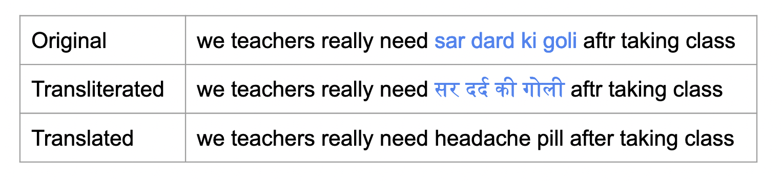
Figure 1: An example of code-switched text where words in both the languages together represent the sentiment. A code-switched text generally contains phrases from multiple languages in a single sentence. The text in blue are words in Hindi that have been written in the Latin script.

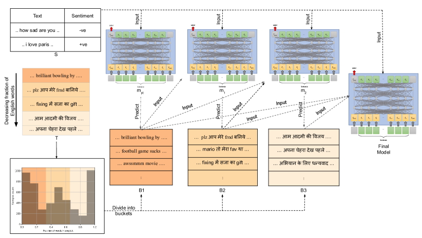
Figure 2: A visualization of the progressive training strategy. The source labelled dataset $S$ in resource rich language should be easily available. Using $S$, a classifier is trained, say $m_{pt}$. Unlabelled code-switched dataset $T$ is divided into buckets using the fraction of English words as the metric. The leftmost bucket B1 has samples dominated by resource-rich language and as we move towards right, the samples in the buckets are dominated by low-resource language. $m_{pt}$ is used to generate pseudo-labels for unlabelled texts in bucket B1. We use texts from B1 along with their pseudo-labels and the dataset $S$ to train a second text classifier $m_{1}$. Then, $m_{1}$ is used to get the pseudo-labels for texts in bucket B2. We keep repeating this until we obtain the final model which is used for predictions.

Intuitively, multilingual language models like mBERT (Devlin et al., 2019) can be used for code-switched text since a single model learns multilingual representations. Although the idea seems straightforward, there are multiple issues. Firstly, mBERT performs differently on different languages depending on their script, prevalence and predominance. mBERT performs well in medium-resource to high-resource languages, but is outperformed by non-contextual subword embeddings in a low-resource setting (Heinzerling and Strube, 2019). Moreover, the performance is highly dependent on the script Pires et al. (2019a). Secondly, pre-trained language models have only seen monolingual sentences during the unsupervised pretraining, however code-switched text contains phrases from both the languages in a single sentence as shown in Figure 1, thus making it an entirely new scenario for the language models. Thirdly, there is difference in the languages based on the amount of unsupervised corpus that is used during pretraining. For e.g., mBERT is trained on the wikipedia corpus. English has $\sim$ 6.3 million articles, whereas Hindi and Tamil have only $\sim$ 140K articles each. This may lead to under-representation of low-resource langauges in the final model. Further, English has been extensively studied by NLP community over the years, making the supervised data and tools more easily accessible. Thus, the model would be able to easily learn patterns present in the resource-rich language segments and motivating us to attempt transfer learning from English supervised datasets to code-switched datasets.

The main idea behind our paper can be summarised as follows: When doing zero shot transfer learning from a resource-rich language (LangA) to code switched language (say LangA-LangB, where LangB is a low-resource language compared to LangA), the model is more likely to be wrong when the instances are dominated by LangB. Thus, instead of self-training on the entire corpus at once, we propose to progressively move from LangA-dominated instances to LangB-dominated instances while transfer learning. As illustrated in Figure 2, model trained on the annotated resource-rich language dataset is used to generate pseudo-labels for code-switched data. Progressive training uses the resource-rich language dataset and (unlabelled) resource-rich language dominated code-switched samples together to generate better quality pseudo-labels for (unlabelled) low-resource language dominated code-switched samples. Lastly, annotated resource-rich language dataset and pseudo-labelled code-switched data are then used together for training which increases the performance of the final model.

Our key contributions are summarized as:

• We propose a simple, novel training strategy that demonstrates superior performance. Since our hypothesis is based on the pretraining phase of the multilingual language models, it can be combined with any transfer learning method.

• We conduct experiments across multiple language-pair datasets, showing efficiency of our proposed method.

• We create probing experiments that verify our hypothesis.

Reproducibility. Our code is publicly available on github .

2 Related work

Multiple tasks like Language Identification, Named Entity Recognition, Part-of-Speech, Sentiment Analysis, Question Answering and NLI have been studied in the code-switched setting. For sentiment analysis,  Vilares et al. (2015) showed that multilingual approaches can outperform pipelines of monolingual models on code-switched data.  Lal et al. (2019) use CNN based network for the same.  Winata et al. (2019) use hierarchical meta embeddings to combine multilingual word, character and sub-word embeddings for the NER task. Aguilar and Solorio (2020) augment morphological clues to language models and uses them for transfer learning from English to code-switched data with labels.  Samanta et al. (2019) uses translation API to create synthetic code-switched text from English datasets and use this for transfer learning from English to code-switched text without labels in the code-switched case. Qin et al. (2020) use synthetically generated code-switched data to enhance zero-shot cross-lingual transfer learning. Recently, Khanuja et al. (2020) released the GLUECoS benchmark to study the performance of multiple models for code-switched tasks across two language pairs En-Es and En-Hi. The benchmark contains 6 tasks, 11 datasets and has 8 models for every task. Multilingual transformers fine tuned with masked-language-model objective on code-switched data can outperform generic multilingual transformers. Results from  Khanuja et al. (2020) show that sentiment analysis, question answering and NLI are significantly harder than tasks like NER, POS and LID. In this work, we focus on the sentiment analysis task in the absence of labeled code-switched data using multilingual transformer models, while taking into account the distinction between resource-rich and low-resource languages. Although our work seems related to curriculum learning, it is distinct from the existing work. Most of the work in curriculum learning is in supervised setting Zhang et al. (2019); Xu et al. (2020) and our work focuses on zero-shot setting, where no code-switched sample is annotated. Note that, this is also different from semi-supervised setting because of distribution shifts between labeled resource-rich language data and target unlabeled code-switched data.

3 Preliminaries

Our problem is a sentiment analysis problem where we have a labelled resource-rich language dataset and unlabelled code-switched data. From here onwards, we refer the labelled resource-rich language dataset as the source dataset and the unlabelled code-switched dataset as target dataset. Since code-switching often occurs in language pairs that include English, we refer to English as the resource-rich language. The source dataset, say $S$, is in English and has the text-label pairs $\{(x_{s_{1}},y_{s_{1}}),(x_{s_{2}},y_{s_{2}}),...(x_{s_{m}},y_{s_{m}})\}$ and the target dataset, say $T$, is in code-switched form and has texts $\{x_{cs_{1}},x_{cs_{2}},...x_{cs_{n}}\}$, where $m$ is significantly greater than $n$. The objective is to learn a sentiment classifier to detect sentiment of code-switched data by leveraging labelled source dataset and unlabelled target dataset.

4 Methodology

Our methodology can be broken down into three main steps: (1) Source dataset pretraining, which uses the resource-rich language labelled source dataset $S$ for training a text classifier. This classifier is used to generate pseudo-labels for the target dataset $T$. (2) Bucket creation, which divides the unlabelled data $T$ into buckets based on the fraction of words from resource-rich language. Some buckets would contain samples that are more resource-rich language dominated while others contain samples dominated by low-resource language. (3) Progressive training, where we initially train using $S$ and the samples dominated by resource-rich language and gradually include the low-resource language dominated instances while training. For rest of the paper, pretraining refers to step 1 and training refers to the training in step 3. And, we also use class ratio based instance selection to prevent the model getting biased towards majority label.

4.1 Source Dataset Pretraining

Resource-rich languages have abundant resources which includes labeled data. Intuitively, sentences in $T$ that are similar to positive sentiment sentences in $S$ would also be having positive sentiment (and same for the negative sentiment). Therefore, we can treat the predictions made on $T$ by multilingual model trained on $S$ as their respective pseudo-labels. This would assign noisy pseudo-labels to unlabeled dataset $T$. The source dataset pretraining step is a text classification task. Let the model obtained after pretraining on dataset $S$ be called $m_{pt}$. This model is used to generate the initial pseudo-labels and to select the instances to be used for progressive training.

4.2 Bucket Creation

Since progressive training aims to gradually progress from training on resource-rich language dominated samples to low-resource language dominated samples, we divide the dataset $T$ into buckets based on fraction of words in resource-rich language. This creates buckets that have more resource-rich language dominated instances and also buckets that have more low-resource language dominated instances as well. In Figure 2, we can observe that the instances in the leftmost bucket are dominated by the English, whereas the instances in the rightmost bucket are dominated by Hindi. More specifically, we define:

$f_{eng}(x_{i})=\frac{n_{eng}(x_{i})}{n_{words}(x_{i})}$

where $n_{eng}(x_{i})$ and $n\_{words}(x_{i})$ denotes the number of English words and total number of words in the text $x_{i}$. Then, we sort the texts in dataset $T$ in decreasing order of $f_{eng}(x_{i})$ and create $k$ buckets $(B_{1},...,B_{k})$ with equal number of texts in each bucket. Thus, bucket $B_{1}$ contains the instances mostly dominated by English language and as we move towards buckets with higher index, instances would be dominated by the low-resource language.

Input: Source dataset $S$, target dataset $T$

Parameter: Selection fraction $\delta$, number of buckets $k$

Output: Predictions on target dataset $T$

Model $m_{bb}$ $\epsilon$ $(mBERT,MuRIL,IndicBERT)$

Model $m_{pt}$ $\leftarrow$ $m_{bb}$ trained on dataset $S$

// Bucketing step

$T^{\prime}$ $\leftarrow$ (($f_{eng}(x_{i})$, $x_{i}$, $m_{pt}(x_{i})$) for $x_{i}$ in $T$)

$T^{\prime}$ $\leftarrow$ $reverse\_sorted(T^{\prime})$

$(B_{1},B_{2},...,B_{k})$ $\leftarrow$ divide $T^{\prime}$ into $k$ equal buckets

// Class ratio based instance selection

$X_{st}=\phi$

for $\mathbf{i}=0,1$ do

       $X_{class_{i}}$ $\leftarrow$ Samples in $T^{\prime}$ predicted to be in class $i$ using $m_{pt}$

       $X_{st}=X_{st}$ $\cup$ ($\delta$ most confident samples in $X_{class_{i}}$)

      

// Progressive training step

Model $m_{0}\leftarrow m_{pt}$

for $\mathbf{i}=1$ to $k$ do

       $X_{st_{i}}$ $\leftarrow$ $X_{st}\cap B_{i}$

       $T_{i}$ $\leftarrow$ $\cup_{r=1}^{r=i}$($(x,m_{r-1}(x))$ for $x$ in $X_{st_{r}}$)

       Model $m_{i}$ $\leftarrow$ $m_{bb}$ trained on $S\cup T_{i}$

Return $m_{k}(T)$

Algorithm 1 Pseudocode for our progressive training framework.

4.3 Progressive Training

As the model $m_{pt}$ is obtained by fine-tuning on a resource-rich language dataset $S$, it is more likely to perform better on resource-rich language dominated instances. Therefore, we choose to start progressive training from resource-rich language dominated samples. However, note that the pseudo-labels generated for dataset $T$ are noisy, thus we sample high confident resource-rich language dominated samples to obtain better quality pseudo-labels for the rest of the instances.

Firstly, we use $m_{pt}$ to obtain all the high confidence samples from dataset $T$ to be used for progressive training and their respective pseudo-labels. Among the samples to be used for progressive training, we select the samples from $B_{1}$ and use them along with $S$ to train a second classifier which is further used to generate pseudo-labels for the rest of the samples to be used for progressive training. Then we select samples from $B_{2}$ and use them along with samples from previous iterations (i.e. samples selected from $B_{1}$ and $S$) to get a third classifier. We continue this process until we reach the last bucket and use the model obtained at the last iteration to make the final predictions.

More formally, we use $m_{pt}$ to select the most confident $\delta$ fraction of samples from the dataset $T$, considering probability as the proxy for the confidence. Let $X_{st}$ denote the $\delta$ fraction of samples with the highest probability of the majority class to be used for progressive training. Let $X_{st_{i}}=X_{st}\cap B_{i}$, where $X_{st_{i}}$ is the subset of samples from bucket $B_{i}$ that would be used for the progressive training. To train across $k$ buckets, we use $k$ iterations. Let $m_{j}$ denote the model obtained after training for iteration $j$ and $m_{0}$ refers to model $m_{pt}$. Iteration $j$ is trained using texts $((\cup_{i=1}^{j}X_{st_{i}})\cup S)$. The true labels for texts in $S$ are available and for texts $X_{st_{i}}$, predictions obtained using model $m_{i-1}$ are considered as their respective labels. The model obtained at the last iteration i.e. $m_{k}$ is used for final predictions.

4.4 Class ratio based instance selection

Datasets frequently have a significant amount of class imbalance. Therefore, when selecting the samples for progressive training, we often end up selecting a very small amount or no samples from the minority class which leads to very poor performance. Hence, instead of selecting $\delta$ fraction of samples from the entire dataset $T$, we select $\delta$ fraction of samples per class. Specifically, let $X_{+}$ and $X_{-}$ denote the set of samples for which the pseudo-labels are positive and negative sentiment respectively. For progressive training, we choose $\delta$ fraction of most confident samples from $X_{+}$ and $\delta$ fraction of most confident samples from $X_{-}$.

The pseudo-code for algorithm is in Algorithm 1.

5 Experiments

We describe the details relevant to the experiments in this section and also elaborate on the probing tasks.

5.1 Datasets

For source dataset pretraining, we use the English Twitter dataset from SemEval 2017 Task 4  (Rosenthal et al., 2017). We use three code-switched datasets for our experiments : Hindi-English  (Patra et al., 2018), Spanish-English  (Vilares et al., 2016), and Tamil-English  (Chakravarthi et al., 2016). Hindi-English, Spanish-English are collected from Twitter and the Tamil-English is collected from YouTube comments. The statistics of the dataset can be found in Table 1. Two out of the three datasets have a class imbalance, the maximum being in the case of Tamil-English where the positive class is $\sim$5x of the negative class. We upsample the minority class to create a balanced dataset.

Most of the sentences in the datasets are written in the Roman script. The words in Hindi and Tamil are converted into the Devanagari script. We use the processed dataset provided by Khanuja et al. (2020) for Hindi-English and Spanish-English datasets. The processed version of Hindi-English dataset has the Hindi words in Devanagari script. Since we deal with low-resource languages for which tools might not be well developed, we use heuristics to detect the words in English. For Spanish-English and Tamil-English datasets, we use the Brown corpus from NLTK to detect the English words in the sentence. Words that are not present in the corpus are considered of another language. For the Tamil-English dataset, we use the AI4Bharat Transliteration python library to get the transliterations.

Table 1: Statistics of datasets. SemEval2017 is a supervised English dataset and the rest are code-switched datasets.

Dataset	Total	Positive	Negative
SemEval2017	27608	19799	7809
Spanish-English	914	489	425
Hindi-English	6190	3589	2601
Tamil-English	10097	8484	1613

5.2 Model training

In all the experiments we use multilingual-bert-base-cased (mBERT) classifier. The supervised English dataset has a 80-20 train-validation split. Following  Wang et al. (2021), $\delta$ is set to $0.5$. We observe that in most datasets, the number of spikes in the distribution plot of $f_{eng}(x_{i})$ is either 1 or 2. For example, we observe there are only two spikes for the Hindi-English dataset in Figure 7 in Appendix A.2. Therefore, we set $k$=2. We train the classifier in both pre-training and training phase for 4 epochs. During pretraining with supervised English dataset, we choose the best weights using the validation set. While training, we use the weights obtained after fourth epoch. For final evaluation, we use the model obtained from the last iteration. Additional details about the hyper-parameters can be found in Appendix A.1.

In the rest of the paper, we refer to the model pretrained on the resource-rich language source dataset as model $m_{pt}$, the model trained on source dataset along with bucket $B_{1}$ as $m_{1}$, and the model trained on source dataset along with the buckets $B_{1}$ and $B_{2}$ as $m_{2}$. $m_{2}$ is used for final predictions.

5.3 Evaluation

As the datasets are significantly skewed between the two classes, we choose to report micro, macro and weighted f1 scores as done in  Mekala and Shang (2020). For code-switched datasets, we use all the samples without labels during the self-training. The final score is obtained using the predictions made by model $m_{2}$ on all the samples and their true labels. For each dataset, we run the experiment with 5 seeds and report the mean and standard deviation.

Table 2: Model performance on the Spanish-English, Hindi-English & Tamil-English dataset using mBERT. For Tamil-English dataset, the - Ratio method increases the F1 score of positive class (which is the majority class) by $\sim 2\%$ but F1 score of negative class drops by $\sim 9\%$. Thus, we observe a performance improvement in weighted F1 score and micro F1 score but a decrease in macro F1 score.

Methods	Spanish-English			Hindi-English			Tamil-English
	Macro-F1	Micro-F1	Weighted-F1	Macro-F1	Micro-F1	Weighted-F1	Macro-F1	Micro-F1	Weighted-F1
Supervised	$71.1$	$71.5$	$71.6$	$74.7$	$74.9$	$75.1$	$62.7$	$84.3$	$82.8$
DEC	$75.7\pm 0.4$	$75.3\pm 0.3$	$75.5\pm 0.5$	$66.0\pm 0.5$	$67.9\pm 0.7$	$67.1\pm 0.4$	$51.7\pm 0.9$	$77.8\pm 0.8$	$75.5\pm 0.6$
No-PT	$76.2\pm 0.6$	$76.3\pm 0.6$	$76.3\pm 0.6$	$67.1\pm 0.8$	$69.2\pm 0.3$	$68.4\pm 0.6$	$53.3\pm 0.4$	$78.6\pm 0.6$	$76.7\pm 0.2$
ZS	$76.1\pm 0.7$	$76.2\pm 0.7$	$76.0\pm 0.7$	$63.8\pm 0.9$	$67.4\pm 0.3$	$65.6\pm 0.7$	$52.7\pm 0.6$	$79.1\pm 0.1$	$76.3\pm 0.2$
Unsup-ST	$73.9\pm 1.7$	$74.3\pm 1.6$	$74.1\pm 1.7$	$66.6\pm 1.5$	$66.7\pm 1.4$	$66.8\pm 1.3$	$49.8\pm 2.1$	$69.2\pm 5.3$	$69.8\pm 8.4$
Ours	$\mathbf{77.4\pm 0.8}$	$\mathbf{77.5\pm 0.8}$	$\mathbf{77.5\pm 0.8}$	$\mathbf{67.8\pm 0.8}$	$\mathbf{69.9\pm 0.5}$	$\mathbf{69.1\pm 0.7}$	$\mathbf{53.1\pm 0.4}$	$80.5\pm 0.2$	$77.5\pm 0.1$
- Source	$76.5\pm 0.7$	$76.7\pm 0.6$	$76.6\pm 0.7$	$67.2\pm 0.5$	$68.7\pm 0.4$	$68.3\pm 0.4$	$52.7\pm 0.7$	$79.2\pm 1.0$	$76.8\pm 0.6$
- Ratio	$77.1\pm 0.7$	$77.3\pm 0.6$	$77.2\pm 0.6$	$64.7\pm 0.5$	$68.4\pm 0.2$	$66.5\pm 0.4$	$49.9\pm 0.3$	$\mathbf{83.3\pm 0.1}$	$\mathbf{77.7\pm 0.1}$

5.4 Baselines

We consider four baselines as described below:

• Deep Embedding for Clustering (DEC)  (Xie et al., 2016) has been used in WeSTClass  (Meng et al., 2018) for self-training using unlabeled documents after pretraining on generated pseudo documents. We adapt DEC similarly to our setting, by pretraining on $S$ and self-training using DEC objective only on $T$.

• No Progressive Training (No-PT) initially trains the model on the source dataset $S$. As done in  (Wang et al., 2021), it selects $\delta$ fraction of the code-switched data with pseudo-labels and trains a classifier on selected samples and the source dataset $S$ without any progressive training.

• Unsupervised Self-Training (Unsup-ST) Gupta et al. (2021) starts with a pretrained sentiment analysis model and then self-trains using code-switched dataset. We use the default version which doesn’t require human annotations. We use the model $m_{pt}$ to initiate the self-training for fair comparison.

• Zero shot (ZS)  (Pires et al., 2019b) denotes the zero shot performance when the model is pretrained on monolingual resource-rich language dataset $S$.

We also compare with two ablation versions of our method, denoted by - Source and - Ratio. - Source uses only the code-switched dataset with its corresponding pseudo-labels without the source dataset $S$ for training. - Ratio chooses the most confident samples for training without taking the class ratio into account.

We also report the performance in the supervised setting, denoted by Supervised. For each dataset, we train the model only on dataset $T$ but use true labels to do the same. This is the possible upper bound.

5.5 Performance comparison

The results for all the three datasets are reported in Table 2. In almost all the cases, we observe a performance improvement using our method as compared to the baselines, maximum improvement being upto $\sim 1.2\%$ in the case of Spanish-English. The comparison between ZS and our method shows the necessity of target code-switched dataset and the comparison between No-PT and our method shows that progressive training has a positive impact. In most cases, the final performance is within $\sim 10\%$ of the supervised setting. We believe our improvements are significant since the baselines are close to the supervised model in terms of the performance and yet our progressive training strategy makes a significant improvement. We report the statistical significance test results between our method and other baselines in Table 8 in Appendix A.4. In all the cases, we observe the p-value to be less than 0.001. The progressively trained model for Spanish-English does better than its corresponding supervised setting, outperforming it by $\sim 6\%$. We hypothesize, this is because of having a large number of instances in the source dataset $S$, the progressively trained model has access to more information and successfully leveraged it to improve the performance on target code-switched dataset. The comparison between our method and its ablated version - Source demonstrates the importance of source dataset while training the classifier. We can note that our proposed method is efficiently transferring the relevant information from the source dataset to the code-switched dataset, thereby improving the performance. On comparing our method with - Ratio, we observe that using class ratio based instance selection improves the performance in two out of three cases. For the Tamil-English dataset, we observe that the weighted & micro F1 score are higher for - Ratio method but the macro F1 score is poor. This is because the F1 score of the positive class increases by $\sim 2\%$ but F1 score of negative class drops by $\sim 9\%$ when using - Ratio method instead of ours. Since the datatset is skewed in the favor of the positive class, this lead to a higher weighted and micro F1 score.

5.6 Performance comparison across buckets

In Figure 3, we plot the performance obtained by No-PT and our method on both buckets. Since our method aims at improving the performance of low-resource language dominated instances, we expect our model $m_{2}$ to perform better on bucket $B_{2}$ and we observe the same. As shown in Figure 3, in most of the cases, our method performs better than the baseline on bucket $B_{2}$. For bucket $B_{1}$, we observe a minor improvement in the case of Spanish-English, whereas it stays similar for other datasets. Detailed qualitative analysis is present in Appendix A.5.

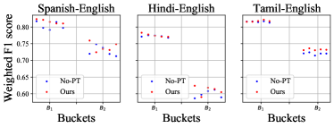
Figure 3: Model performance comparison across buckets. $B_{1}$ contains English dominated instances and $B_{2}$ contains low resource language dominated instances. Values are reported across 5 runs. Points on the same vertical line are from the same run i.e. both No-PT and our model were initialized with same initial weights.

5.7 Probing task : Out-Of-Distribution (OOD) detection

As previously mentioned, our proposed framework is based on two main hypotheses: (1.) A transformer model trained on resource-rich language dataset is more likely to be correct/robust on resource-rich language dominated samples compared to the low-resource language dominated samples, (2.) The models obtained using the progressive training framework is more likely to be correct/robust on the low-resource dominated samples compared to the models self-trained on the entire code-switched corpus at once. To confirm our hypotheses, we perform a probing task where we compute the fraction of the samples that are OOD. More specifically, we ask two questions: a) Is the fraction of OOD samples same for both the buckets for model $m_{pt}$? b) Is there a change in OOD fraction for bucket $B_{2}$ if we use model $m_{1}$ instead of model $m_{pt}$? The first question helps in verifying the first part of the hypothesis and the second question helps in verifying the second part of the hypothesis.

Since the source dataset $S$ is in English and the target dataset $T$ is code-switched, the entire dataset $T$ might be considered as out-of-distribution. However, transformer models are considered robust and can generalise well to OOD data  (Hendrycks et al., 2020). Determining if a sample is OOD is difficult until we know more about the difference in the datasets. However, model probability can be used as a proxy. We use the method based on model’s softmax probability output similar to  Hendrycks and Gimpel (2018) to do OOD detection. Higher the probability of the predicted class, more is the confidence of the model, thus less likely the sample is out of distribution.

For a given model trained on a dataset, a threshold $p_{\alpha}$ is determined using the development set (or the unseen set of samples) to detect OOD samples. $p_{\alpha}$ is the probability value such that only $\alpha$ fraction of samples from the development set (or the unseen set of samples) have probability of the predicted class less than $p_{\alpha}$. For example, if $\alpha=10\%$, $90\%$ of samples in the development set have probability of predicted class greater than $p_{\alpha}$. If a new sample from another dataset (or bucket) has probability of predicted class less than $p_{\alpha}$, we would consider it to be OOD. Using $p_{\alpha}$, we can determine the fraction of samples from the new set that are OOD. Since, there is no method to know the exact value of $\alpha$ to be used, we report OOD using three values of $\alpha$ : 0.01, 0.05 and 0.10. For model $m_{pt}$, we use the development split from the dataset $S$ to determine the value of $p_{\alpha}$, and for model $m_{1}$, we use the set of samples from bucket $B_{1}$ that are not used in self-training (i.e. $B_{1}-X_{st_{1}}$) to determine $p_{\alpha}$. Based on the value of $\alpha$, we conduct two experiments and answer our two questions.

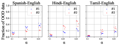
Figure 4: Figure showing bucketwise OOD for different datasets using the model $m_{pt}$. In most cases, samples in $B_{2}$ are more OOD compared to samples in $B_{1}$ across different values of $\alpha$. Values are reported across 5 runs, points on the same vertical line are from the same run i.e. once a model $m_{pt}$ has been trained, the same model is used to evaluate the fraction of OOD data in both the buckets.

Table 3: Performance using multiple multilingual models. First three rows denote performance without using progressive training and the last row denotes the performance when the model with best performance is used with progressive training.

Model	Spanish-English			Hindi-English			Tamil-English
	Macro-F1	Micro-F1	Weighted-F1	Macro-F1	Micro-F1	Weighted-F1	Macro-F1	Micro-F1	Weighted-F1
mBERT	$76.2\pm 0.6$	$76.3\pm 0.6$	$76.3\pm 0.6$	$67.1\pm 0.8$	$69.2\pm 0.3$	$68.4\pm 0.6$	$53.3\pm 0.4$	$78.6\pm 0.6$	$76.7\pm 0.2$
MuRIL	-	-	-	$\mathbf{77.0\pm 0.4}$	$\mathbf{77.7\pm 0.3}$	$\mathbf{77.7\pm 0.4}$	$54.2\pm 0.2$	$64.2\pm 0.4$	$68.8\pm 0.3$
IndicBERT	-	-	-	$73.5\pm 0.5$	$74.5\pm 0.3$	$74.3\pm 0.4$	$\mathbf{54.6\pm 0.1}$	$68.0\pm 0.6$	$71.3\pm 0.4$
Ours + Best	$\mathbf{77.4\pm 0.8}$	$\mathbf{77.5\pm 0.8}$	$\mathbf{77.5\pm 0.8}$	$\mathbf{77.0\pm 0.4}$	$77.6\pm 0.4$	$77.6\pm 0.4$	$53.1\pm 0.4$	$\mathbf{80.5\pm 0.2}$	$\mathbf{77.5\pm 0.1}$

Table 4: Model performance on the three datasets for different number of buckets ($k$) using mBERT.

Buckets	Spanish-English			Hindi-English			Tamil-English
	Macro-F1	Micro-F1	Weighted-F1	Macro-F1	Micro-F1	Weighted-F1	Macro-F1	Micro-F1	Weighted-F1
k=2	$\mathbf{77.4\pm 0.8}$	$\mathbf{77.5\pm 0.8}$	$\mathbf{77.5\pm 0.8}$	$\mathbf{67.8\pm 0.8}$	$\mathbf{69.9\pm 0.5}$	$\mathbf{69.1\pm 0.7}$	$\mathbf{53.1\pm 0.4}$	$80.5\pm 0.2$	$\mathbf{77.5\pm 0.1}$
k=3	$76.1\pm 0.7$	$76.2\pm 0.7$	$76.2\pm 0.7$	$67.2\pm 0.6$	$69.4\pm 0.5$	$68.6\pm 0.6$	$53.1\pm 0.2$	$79.9\pm 0.4$	$77.2\pm 0.1$
k=4	$76.6\pm 1.6$	$76.7\pm 1.7$	$76.7\pm 1.6$	$67.6\pm 0.4$	$69.7\pm 0.3$	$68.9\pm 0.4$	$52.9\pm 0.4$	$\mathbf{80.6\pm 0.7}$	$\mathbf{77.5\pm 0.3}$

Is the fraction of OOD samples same for both the buckets for model $m_{pt}$? In the first experiment, we consider the model trained on the source dataset and try to find the fraction of OOD samples in both the buckets. Since the first bucket contains more resource-rich language dominated samples, we expect a lesser fraction of samples to be out-of-distribution compared to the second bucket. In Figure 4, we plot the bucketwise OOD for different datasets. We observe that lesser fraction of samples from first bucket are OOD in all the datasets except Spanish-English. This shows that instances dominated by resource-rich language are less likely to be out-of-distribution for the classifier trained on $S$ compared to instances dominated by low-resource language, thus providing empirical evidence in support of the first part of our hypothesis. We also report the zero-shot performance in Appendix A.3 i.e. we use the classifier trained on source dataset for inference with no training on target dataset. For all the datasets, we observe zero-shot model performs better on $B_{1}$ compared to $B_{2}$, thus further bolstering our hypothesis.

Figure 5: Figure showing model wise OOD for bucket $B_{2}$ across multiple datasets. We compare two models, $m_{pt}$ and $m_{1}$. In all the cases, we observe that samples in $B_{2}$ are more OOD for model $m_{pt}$ compared to $m_{1}$ across different values of $\alpha$. Values are reported for 5 runs and points on the same vertical line are from the same run i.e. both $m_{pt}$ and $m_{1}$ were initialized with same initial weights.

Is there a change in OOD fraction for bucket $B_{2}$ if we use model $m_{1}$ instead of model $m_{pt}$?

In the second experiment, we compare the fraction of OOD data in bucket $B_{2}$ for the models $m_{pt}$ and $m_{1}$.

In Figure 5, we observe a lesser fractions of samples in bucket B2 are OOD for model $m_{1}$ compared to model $m_{pt}$. This is expected since the model $m_{1}$ has seen samples with low-resource language words while training, thus providing empirical evidence in the support of our proposed training strategy. Although, the samples from $B_{2}$ would still have noisy labels, we expect them to be more accurate when predicted by $m_{1}$ than $m_{pt}$.

5.8 Comparison with other multilingual models

Recently, multiple multilingual transformer models have been proposed. We experiment with MuRIL (Khanuja et al., 2021) and IndicBERT (Kakwani et al., 2020). Firstly, we obtain the performance of three language models: mBERT, MuRIL, and IndicBERT without progressive training on all datasets and we use progressive training on top of the best performing model corresponding to each dataset and verify whether it further improves the performance. The F1 scores are reported in Table 3. We observe that performance either increases or stays very competitive in all the cases, thus showing our method is capable of improving performance even when used with the best multilingual model for the task.

5.9 Hyper-parameter sensitivity analysis

There are two hyper-parameters in our experiments: the number of buckets ($k$) and the ratio of samples selected for self-training ($\delta$). We vary $k$ from 2 to 4 to study the effect of the number of buckets on the performance and the F1-scores are reported in Table 4. Our method is fairly robust to the values of k. For almost all values of k, our method does better than the baselines. As mentioned earlier, the number of spikes in the distribution plot of $f_{eng}$ is 1 or 2 for all the datasets. In presence of more number of spikes, higher value of $k$ is recommended.

Figure 6: F1 score using different values of parameter $\delta$ for the three datasets (Spanish-English, Hindi-English and Tamil-English). The plots represent macro, micro and weighted F1 score (left-to-right).

For studying the effect of hyper-parameter $\delta$, we plot macro, micro, and weighted F1 scores across multiple values of $\delta$ in Figure 6. With low $\delta$, there wouldn’t be enough sentences for self-training to help whereas with high $\delta$, the samples would be too noisy. Thus, a value in the middle i.e. 0.4-0.6 should be reasonable choice.

6 Conclusion and Future work

In this paper, we propose progressive training framework that takes distinction between low-resource and resource-rich language into account while doing zero-shot transfer learning for code-switched sentiment analysis. We show that our framework improves performance across multiple datasets. Further, we also create probing tasks to provide empirical evidence in support of our hypothesis. In future, we want to extend the framework to other tasks like question-answering and natural language inference.

7 Limitations

A key potential limitation of the current framework is that if the number of samples in buckets are very disproportionate, the progressive learning might not result in significant improvement.

8 Ethical consideration

This paper proposes a progressive training framework to transfer knowledge from resource-rich language data to low-resource code-switched data. We work on sentiment classification task which is a standard NLP problem. Based on our experiments, we don’t see any major ethical concerns with our work.

9 Acknowledgements

We thank Zihan Wang for valuable discussions and comments. Our work is sponsored in part by National Science Foundation Convergence Accelerator under award OIA-2040727 as well as generous gifts from Google, Adobe, and Teradata. Any opinions, findings, and conclusions or recommendations expressed herein are those of the authors and should not be interpreted as necessarily representing the views, either expressed or implied, of the U.S. Government. The U.S. Government is authorized to reproduce and distribute reprints for government purposes not withstanding any copyright annotation hereon.

Appendix A Appendix

A.1 Additional hyper-parameter details

The batch size is 64, sequence length is 128 and learning rate is 5e-5. These hyperparameters are same for all the models used during pre-training and training. Every iteration takes approximately $\sim$1-2 seconds and $\sim$12 GB of memory on a GPU.

A.2 Statistics related to the buckets

We report the average value and standard deviation of the $f_{eng}$ across the buckets in Table 5. We report the number of instances selected for self-training across the buckets in Table 6. We plot the distribution of $f_{eng}$ in Figure 7.

Table 5: Average value and standard deviation of $f_{eng}$ for both the buckets $B_{1}$ and $B_{2}$.

Dataset	$B_{1}$	$B_{2}$
Spanish-English	$0.79\pm 0.08$	$0.44\pm 0.14$
Hindi-English	$0.79\pm 0.21$	$0.14\pm 0.13$
Tamil-English	$0.51\pm 0.16$	$0.13\pm 0.09$

Table 6: Number of samples selected from each bucket B1 and B2 for progressive training.

Dataset	$B_{1}$	$B_{2}$
Spanish-English	265	191
Hindi-English	2047	1048
Tamil-English	2877	2169

Figure 7: Distribution of $f_{eng}(x)$ vs number of samples for the Spanish-English, Hindi-English and Tamil-English datasets (left-to-right). For Hindi-English, we can observe two spikes in the graph showing some samples are heavily dominated by English and some samples are heavily dominated by Hindi. For the other two datasets, we observe the progression to be more gradual.

A.3 Results of the zero-shot model on buckets

We report the results of the zero-shot model on both the buckets in Table 7. As expected, in all the cases the model performs better on $B_{1}$ compared to $B_{2}$.

Table 7: Bucketwise results of the zero-shot model. Macro, Micro and Wtd refer to Macro-F1, Micro-F1 and Weighted-F1 scores respectively.

	$B_{1}$			$B_{2}$
Dataset	Macro	Micro	Wtd	Macro	Micro	Wtd
Spanish-English	79.2	79.6	79.7	71.8	73.3	73.8
Hindi-English	73.9	77.6	76.9	56.0	58.0	56.2
Tamil-English	54.6	83.4	81.6	50.6	77.0	72.8

A.4 Statistical Significance Results

Table 8: We perform paired t-test between our method and baselines. The p-value obtained by performing the test between our methods and baselines for all three datasets is reported in the table.

Dataset	No-PT	DCE	- Source	- Ratio
Spanish-English	$5.11e^{-13}$	$2.09e^{-6}$	$8.28e^{-4}$	$8.82e^{-8}$
Hindi-English	$2.76e^{-6}$	$4.37e^{-43}$	$3.49e^{-4}$	$6.85e^{-12}$
Tamil-English	$1.87e^{-41}$	$3.72e^{-16}$	$3.71e^{-3}$	$3.40e^{-7}$

A.5 Qualitative analysis

As discussed previously, on the low-resource language dominated bucket, our model is correct more often than the No-PT baseline. We focus on samples from bucket $B_{2}$ for qualitative analysis. For the sample, "fixing me saja hone ka gift", the Hindi word "saja" refers to punishment which is negative in sentiment whereas the word "gift" is positive in sentiment. Thus, the contextual information in the Hindi combined with that of the English is necessary to make correct prediction. For the sample "Mera bharat mahan, padhega India tabhi badhega India", the model has to identify Hindi words "mahan" & "badhega" to make the correct predictions.

We also do the qualitative analysis by looking at predictions of samples between successive iterations. In Table 9, we randomly choose samples which are predicted incorrectly by model $m_{pt}$ but are predicted correctly by model $m_{1}$. Out of 8 samples, 6 samples had sentiment specifically present in the Hindi words. In Table 10, we randomly choose samples which are predicted incorrectly by model $m_{1}$ but are predicted correctly by model $m_{2}$. Out of 8 samples, 4 samples had sentiment specifically present in the Hindi words and 2 samples required understanding both the Hindi and English words simultaneously. The blue highlighted words are relevant to determining the sentiment of the sentence.

Table 9: Instances where model $m_{pt}$ was incorrect but model $m_{1}$ learnt the correct label.

Bucket	Text	Label
0	yes we teachers really need sar dard ki goli aftr taking class	negative
0	they are promising moon right now to get the cm post . . . waade aise hone chahiye jo janta k welfare k liye ho . . . free wahi baantna chahta hai jo desperate ho kisi tarah ek baar bas kursi mil jaye .	negative
0	oooo ! grandfather bas ab nahi kitna natak karoge	negative
0	i agree with this cartoon . bahut achcha doston .	positive
0	seriously maza boht ata tha , , , mere pass mast collection hota tha	positive
1	school mein milne wale laddoo kitni khushi dete they :d	positive
1	guddu itni paas se tv dekhega toh aankhe button ho jayengi !	negative
1	arun lal ki commentary yaad aa gayi . . usse zyada manhoos koi nahi .	negative

Table 10: Instances where model $m_{1}$ was incorrect but model $m_{2}$ learnt the correct label.

Bucket	Text	Label
0	Osm party salman bhai apka gift	positive
0	mat dekho brothers and sisters , dekha nahi jayega	negative
0	Ap late ho ap ne apne cometment pori nai ki	negative
0	looks like ’kaho na pyaar hai’ phase ended for modi #aapsweep #aapkidilli #delhidecides	negative
1	comment krne se jyada sabke padhne me maja aata h	positive
1	guddu tumhara hi school aisa hoga yaar . mera school n mere teacher to ache h	positive
1	sir kya msg krtte kartte mar jau	negative
1	Hum bhuke mur rahe hai sir	negative

References

- Aguilar and Solorio (2020) Gustavo Aguilar and Thamar Solorio. 2020. From English to code-switching: Transfer learning with strong morphological clues. In Proceedings of the 58th Annual Meeting of the Association for Computational Linguistics, pages 8033–8044, Online. Association for Computational Linguistics.
- Chakravarthi et al. (2016) Bharathi Raja Chakravarthi, Ruba Priyadharshini, Vigneshwaran Muralidaran, Navya Jose, Shardul Suryawanshi, Elizabeth Sherly, and John P McCrae. 2016. Dravidiancodemix: Sentiment analysis and offensive language identification dataset for dravidian languages in code-mixed text. Language Resources and Evaluation.
- Devlin et al. (2019) Jacob Devlin, Ming-Wei Chang, Kenton Lee, and Kristina Toutanova. 2019. Bert: Pre-training of deep bidirectional transformers for language understanding.
- Gupta et al. (2021) Akshat Gupta, Sargam Menghani, Sai Krishna Rallabandi, and Alan W Black. 2021. Unsupervised self-training for sentiment analysis of code-switched data. In Proceedings of the Fifth Workshop on Computational Approaches to Linguistic Code-Switching, pages 103–112, Online. Association for Computational Linguistics.
- Heinzerling and Strube (2019) Benjamin Heinzerling and Michael Strube. 2019. Sequence tagging with contextual and non-contextual subword representations: A multilingual evaluation. In Proceedings of the 57th Annual Meeting of the Association for Computational Linguistics, pages 273–291, Florence, Italy. Association for Computational Linguistics.
- Hendrycks and Gimpel (2018) Dan Hendrycks and Kevin Gimpel. 2018. A baseline for detecting misclassified and out-of-distribution examples in neural networks.
- Hendrycks et al. (2020) Dan Hendrycks, Xiaoyuan Liu, Eric Wallace, Adam Dziedzic, Rishabh Krishnan, and Dawn Song. 2020. Pretrained transformers improve out-of-distribution robustness. In Proceedings of the 58th Annual Meeting of the Association for Computational Linguistics, pages 2744–2751, Online. Association for Computational Linguistics.
- Kakwani et al. (2020) Divyanshu Kakwani, Anoop Kunchukuttan, Satish Golla, Gokul N.C., Avik Bhattacharyya, Mitesh M. Khapra, and Pratyush Kumar. 2020. IndicNLPSuite: Monolingual corpora, evaluation benchmarks and pre-trained multilingual language models for Indian languages. In Findings of the Association for Computational Linguistics: EMNLP 2020, pages 4948–4961, Online. Association for Computational Linguistics.
- Khanuja et al. (2021) Simran Khanuja, Diksha Bansal, Sarvesh Mehtani, Savya Khosla, Atreyee Dey, Balaji Gopalan, Dilip Kumar Margam, Pooja Aggarwal, Rajiv Teja Nagipogu, Shachi Dave, Shruti Gupta, Subhash Chandra Bose Gali, Vish Subramanian, and Partha P. Talukdar. 2021. Muril: Multilingual representations for indian languages. CoRR, abs/2103.10730.
- Khanuja et al. (2020) Simran Khanuja, Sandipan Dandapat, Anirudh Srinivasan, Sunayana Sitaram, and Monojit Choudhury. 2020. GLUECoS: An evaluation benchmark for code-switched NLP. In Proceedings of the 58th Annual Meeting of the Association for Computational Linguistics, pages 3575–3585, Online. Association for Computational Linguistics.
- Lal et al. (2019) Yash Kumar Lal, Vaibhav Kumar, Mrinal Dhar, Manish Shrivastava, and Philipp Koehn. 2019. De-mixing sentiment from code-mixed text. In Proceedings of the 57th Annual Meeting of the Association for Computational Linguistics: Student Research Workshop, pages 371–377, Florence, Italy. Association for Computational Linguistics.
- Mekala and Shang (2020) Dheeraj Mekala and Jingbo Shang. 2020. Contextualized weak supervision for text classification. In Proceedings of the 58th Annual Meeting of the Association for Computational Linguistics, pages 323–333, Online. Association for Computational Linguistics.
- Meng et al. (2018) Yu Meng, Jiaming Shen, Chao Zhang, and Jiawei Han. 2018. Weakly-supervised neural text classification. CoRR, abs/1809.01478.
- Patra et al. (2018) Braja Gopal Patra, Dipankar Das, and Amitava Das. 2018. Sentiment analysis of code-mixed indian languages: An overview of sail_code-mixed shared task @icon-2017.
- Pires et al. (2019a) Telmo Pires, Eva Schlinger, and Dan Garrette. 2019a. How multilingual is multilingual bert?
- Pires et al. (2019b) Telmo Pires, Eva Schlinger, and Dan Garrette. 2019b. How multilingual is multilingual bert? CoRR, abs/1906.01502.
- Qin et al. (2020) Libo Qin, Minheng Ni, Yue Zhang, and Wanxiang Che. 2020. Cosda-ml: Multi-lingual code-switching data augmentation for zero-shot cross-lingual nlp. ArXiv, abs/2006.06402.
- Rosenthal et al. (2017) Sara Rosenthal, Noura Farra, and Preslav Nakov. 2017. SemEval-2017 task 4: Sentiment analysis in Twitter. In Proceedings of the 11th International Workshop on Semantic Evaluation (SemEval-2017), pages 502–518, Vancouver, Canada. Association for Computational Linguistics.
- Samanta et al. (2019) Bidisha Samanta, Niloy Ganguly, and Soumen Chakrabarti. 2019. Improved sentiment detection via label transfer from monolingual to synthetic code-switched text. arXiv preprint arXiv:1906.05725.
- Vilares et al. (2015) David Vilares, Miguel A. Alonso, and Carlos Gómez-Rodríguez. 2015. Sentiment analysis on monolingual, multilingual and code-switching Twitter corpora. In Proceedings of the 6th Workshop on Computational Approaches to Subjectivity, Sentiment and Social Media Analysis, pages 2–8, Lisboa, Portugal. Association for Computational Linguistics.
- Vilares et al. (2016) David Vilares, Miguel A. Alonso, and Carlos Gómez-Rodríguez. 2016. EN-ES-CS: An English-Spanish code-switching Twitter corpus for multilingual sentiment analysis. In Proceedings of the Tenth International Conference on Language Resources and Evaluation (LREC’16), pages 4149–4153, Portorož, Slovenia. European Language Resources Association (ELRA).
- Wang et al. (2021) Zihan Wang, Dheeraj Mekala, and Jingbo Shang. 2021. X-class: Text classification with extremely weak supervision. In Proceedings of the 2021 Conference of the North American Chapter of the Association for Computational Linguistics: Human Language Technologies, pages 3043–3053, Online. Association for Computational Linguistics.
- Winata et al. (2019) Genta Indra Winata, Zhaojiang Lin, Jamin Shin, Zihan Liu, and Pascale Fung. 2019. Hierarchical meta-embeddings for code-switching named entity recognition. In Proceedings of the 2019 Conference on Empirical Methods in Natural Language Processing and the 9th International Joint Conference on Natural Language Processing (EMNLP-IJCNLP), pages 3541–3547, Hong Kong, China. Association for Computational Linguistics.
- Xie et al. (2016) Junyuan Xie, Ross Girshick, and Ali Farhadi. 2016. Unsupervised deep embedding for clustering analysis.
- Xu et al. (2020) Benfeng Xu, Licheng Zhang, Zhendong Mao, Quan Wang, Hongtao Xie, and Yongdong Zhang. 2020. Curriculum learning for natural language understanding. In Proceedings of the 58th Annual Meeting of the Association for Computational Linguistics, pages 6095–6104, Online. Association for Computational Linguistics.
- Zhang et al. (2019) Xuan Zhang, Pamela Shapiro, Gaurav Kumar, Paul McNamee, Marine Carpuat, and Kevin Duh. 2019. Curriculum learning for domain adaptation in neural machine translation. In Proceedings of the 2019 Conference of the North American Chapter of the Association for Computational Linguistics: Human Language Technologies, Volume 1 (Long and Short Papers), pages 1903–1915, Minneapolis, Minnesota. Association for Computational Linguistics.