Functional Simulation of
Real-Time Quantum Control Software

Abstract

Modern quantum computers rely heavily on real-time control systems for operation. Software for these systems is becoming increasingly more complex due to the demand for more features and more real-time devices to control. Unfortunately, testing real-time control software is often a complex process, and existing simulation software is not usable or practical for software testing. For this purpose, we implemented an interactive simulator that simulates signals at the application programming interface level. We show that our simulation infrastructure simulates kernels 6.9 times faster on average compared to execution on hardware, while the position of the timeline cursor is simulated with an average accuracy of 97.9% when choosing the appropriate configuration.

I Introduction

State-of-the-art quantum hardware is becoming increasingly powerful with recent systems demonstrating computations on tens of qubits [1, 2, 3, 4, 5, 6, 7]. Recent papers [1, 8, 9, 5] have shown that such systems rely heavily on real-time control systems to control tens to hundreds of devices with nanosecond precision. Programmable real-time control systems, as described in [10, 11, 12, 13, 14], are already available and widely adopted. An often underexposed area of such real-time control systems is the increasingly complex control software required to operate them. Larger quantum systems control more real-time devices, which leads to an increasing amount of software. In addition, real-time software is taking on more responsibilities ranging from hardware latency compensation to decomposing quantum gates into device control which further increases its complexity.

With the growing complexity of real-time control software, functional testing and verification is becoming increasingly important. Unfortunately, testing real-time control software is often complex, time-consuming, and resource-intensive. Testing on hardware requires access to control hardware and test equipment, such as oscilloscopes and signal generators, to probe and stimulate the control system, as illustrated in Figure 1. Even if all required test equipment is available, configuring the equipment to simulate the correct test signals can be complex and time-consuming. Additionally, black-box testing on hardware might not give enough insight into the state of the software if incorrect behavior is observed. Software testing with hardware requires hardware to be available, which might not be the case in the early stages of development. The use of simulation could enable testing of real-time control software, but simulators are usually not available for real-time control systems, as is the case for [10, 11, 12, 13]. Existing simulation approaches that might be available, such as cycle-accurate hardware simulation, often focus on the microarchitectural level. Such simulations are too slow, inflexible, and low-level to be useful for testing real-time control software.

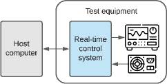
Figure 1: The equipment required for hardware testing, which includes the real-time control system, oscilloscopes, and signal generators.

In this paper, we present an open-source functional simulator for real-time control software targeting the advanced real-time infrastructure for quantum physics (ARTIQ) open-source software and hardware ecosystem [10, 15]. Our interactive simulator simulates all aspects of real-time control software, including classical constructs, real-time events, and device input. Real-time device signals are simulated at the application programming interface (API) level, which enables functional software testing and fast simulation speeds. Our simulator integrates seamlessly into the ARTIQ host environment and is capable of simulating interactions between the host and the real-time control system. With our simulation infrastructure, users can test and verify real-time control software using existing tools for step debugging, unit testing, and continuous integration. Without the need for any of the test hardware shown in Figure 1, our simulator enables software testing in the early development stages. We show that our kernel simulation is on average 6.9 times faster than execution on control hardware. Even with the presence of variable delays and simplified timing models for devices, the position of the timeline cursor is simulated with an average accuracy of 97.9% when appropriately configured.

The remainder of this paper is structured as follows. Section II briefly covers related work, and in Section III we will provide an overview of the ARTIQ hardware and software components that we will simulate. The design of our simulation platform is presented in Section IV, while the results of our performance and accuracy measurements can be found in Section V. We conclude our paper in Section VI.

II Related work

Real-time control hardware and software can be simulated with techniques similar to ones used for the simulation of embedded systems. Previous work such as [16, 17] proposes various techniques and approaches for such simulations. Real-time control hardware can be simulated on a microarchitectural level based on their hardware description using the same binaries as the actual hardware. Cycle-accurate microarchitectural simulations can be performed with tools such as GEM5 [18], SystemC [19, 20], Chisel [21], or SimSoC [22]. Most of these tools can perform low-level and detailed cycle-accurate simulations of the hardware. Unfortunately, cycle-accurate simulations are often not usable for software testing and verification because simulations run slow and the simulated signals are too low-level for testing real-time software and device behavior. These simulations also require detailed device models that might not be available in the early development stages. The same holds for simulation techniques based on communication models of the microarchitecture, such as [17, 23, 24, 22].

High-level simulation approaches for quantum computer architecture as discussed in [25, 26, 27] can be fast and test real-time quantum programs. Unfortunately, these simulators operate on the quantum-gate level and do not simulate the real-time device control required to implement such operations. Hence, high-level simulators are not usable for testing real-time control software on a real-time device and signal level.

III System overview

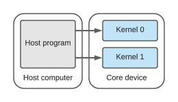
Figure 2: Schematic overview of the accelerator model with a host program and one or more kernels.

Our simulator targets the ARTIQ open-source software and hardware ecosystem [10, 15] which is used by dozens of research groups and has deployed over 200 real-time control systems worldwide. The ARTIQ ecosystem combines a Python-based software environment with modular real-time control hardware, and its programming paradigm is based on the accelerator model as described in [28, 13, 29, 26, 30, 31, 32, 33]. The ARTIQ software environment runs on a host computer that communicates with the control hardware, also referred to as the core device, over ethernet. Users can program the system using a Python host environment while kernels are executed on the core device as illustrated in Figure 2.

III-A Hardware

The core device is driven by a field-programmable gate array (FPGA) which contains a classical CPU combined with an event-based real-time I/O (RTIO) subsystem similar to the systems outlined in [34, 13]. Figure 3 shows a simplified schematic of the relevant microarchitectural components in the FPGA. The classical CPU will handle all classical instructions of the kernel and has additional access to a timeline cursor and an event timeline. The timeline cursor is a register that holds the current position on a timeline. The cursor is stored as an integer value that represents a time in machine units (MU), which normally corresponds to a timestamp expressed in nanoseconds. The CPU can also post events to the event timeline where an event is defined as a tuple of a timestamp and an I/O command. To change the state of a device, the CPU sets the timeline cursor to the time at which the change should occur before posting the I/O command to the event timeline. The current value of the timeline cursor will be used to store the event on the timeline. If the CPU posts two commands for the same device at the same timestamp, the last event will overwrite the first one. By posting a series of events, a program can build up an event timeline that represents the real-time control of devices.

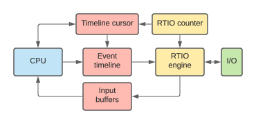
Figure 3: A schematic overview of the microarchitectural components in the core device.

In parallel to the CPU’s execution, the RTIO subsystem continuously verifies if any events are due. The RTIO counter represents a timestamp in MU and is incremented every nanosecond. The RTIO engine reads the event timeline and verifies if any events are due based on the current value of the RTIO counter. If an event is due, the RTIO engine updates the corresponding device according to the command defined by the event. In case an event generates a return value, for example, when reading the value of a digital input, the return value is inserted into the input buffers. The CPU can read results from the input buffers whenever they are available.

For the RTIO system to operate properly, the slack (i.e. the difference between the timeline cursor and the RTIO counter) must be positive. Posting an event with negative slack translates to changing the state of a device in the past, which is not possible. Doing so will result in an underflow exception. Kernels normally start their program by synchronizing the timeline cursor to the RTIO counter and incrementing the timeline cursor with a fixed value of $125\times 10^{3}$ MU to ensure positive slack at the start of the program.

III-B Software

The ARTIQ software environment is Python-based and programs that run on the system are called experiments. An experiment consists of Python code that runs on the host and can additionally contain kernel functions that run on the core device. Kernel functions are written in the ARTIQ domain-specific language (DSL) which is a subset of the Python language. Inside kernels, programmers have access to additional functions to manipulate the timeline cursor, post events, and read input buffers. The latter two are normally not directly used by programmers as these functions are encapsulated in device drivers. Such device drivers provide an API to translate functional device behavior (e.g. switch off a digital output pin) to low-level events. A schematic overview of a host program and a kernel with access to APIs for the timeline cursor and device drivers is shown in Figure 4.

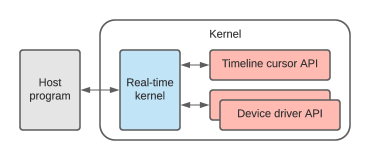
Figure 4: A schematic overview of a host program a kernel with access to APIs for the timeline cursor and device drivers.

When the host calls a kernel function, the ARTIQ compiler assembles a kernel binary at runtime which is then uploaded to and executed by the core device. Variables from the host environment that are accessed in a kernel will be compiled into the binary. During kernel execution, the host will handle any (a)synchronous remote procedure calls initiated by the kernel. Once the kernel is finished executing, the context switches back to the host, and any variables modified in the kernel are synchronized with the host environment before the experiment resumes executing on the host. As a result, the context switch between host and kernel code is almost seamless from a programmer’s perspective.

IV Simulation

Our goal is to enable the simulation of real-time control software for software testing and verification. A simulator should integrate into the existing ARTIQ environment, simulate kernel execution, and simulate any interactions between the host environment and the kernel as described in Section III. The simulator should be fast enough to test complete experiments within a reasonable time. No real-time control hardware should be required to run simulations, only a model of the hardware listing the available devices. Hardware/software co-simulation for embedded systems is not new, and existing work proposes various techniques and approaches for such simulations [16, 17]. At the most detailed level, we find cycle-accurate simulations, such as [18, 19, 21], that take the same binary as the real system and simulate the components and registers of the microarchitecture in great detail. Such simulations require highly detailed models making them inflexible and potentially time-consuming to develop. Cycle-accurate simulators are extremely detailed and accurate but are also slow. It is not our goal to do performance analysis on the ARTIQ microarchitecture, and we do not need such a level of detail. Since our target is software testing and not hardware performance analysis, we will focus on API simulation. An API simulation cross-compiles the target program to a simulator that implements the same API as the target system. The simulator requires no execution model of the hardware and can therefore be fast. Based on our requirements, we decide to target functional simulation of kernels and real-time devices using API simulation. Timeline cursor manipulations will be simulated at the API level. Real-time devices are simulated at their driver API level, and functional behavior will be based on a simplified device model. Hence, we will replace the timeline cursor API and the device driver APIs shown in Figure 4 with calls to our simulation infrastructure. The state of the RTIO counter and RTIO engine are not simulated, which would require the use of a cycle-accurate simulator. Instead, we estimate the value of the RTIO counter when synchronizing the timeline cursor with the RTIO counter.

For simulation of real-time kernels, we will need to cover classical constructs (i.e. the CPU), the timeline cursor, the event timeline, and input buffers. Since both the host code and the classical constructs of the kernels are valid Python code, we decided to use the host Python process to simulate kernels. Hence, our simulator is implemented in Python and all components in Figure 4 will be executed by the Python interpreter. Using the same Python process will also instantly implement host-kernel variable synchronization and handling of RPCs. We decided to split the simulation of the remaining components into two parts: time and signals. The time component covers the simulation of the timeline cursor, and the signals component covers the simulation of the event timeline and input buffers. Figure 5 shows a schematic overview of the simulated components. In the remainder of this section, we will cover time and signal simulation.

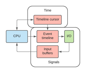
Figure 5: A schematic overview of the simulated microarchitectural components.

IV-A Time

A kernel can read and write the value of the timeline cursor using the functions now_mu() and at_mu(t), respectively. Additionally, the cursor can be moved relative from its current position using the functions delay_mu(d) and delay(d). The latter function is used with a delay time expressed in seconds instead of MU. Since the delay in seconds is converted to a delay in MU, the delay(d) function is not further discussed. Functions used to modify the timeline cursor behave differently depending on the timing context in which they are used. There are two timing contexts, sequential and parallel, which are used as regular Python context managers using the with statement. The two contexts are used to specify if a set of RTIO operations should be executed sequentially or in parallel. The contexts can be nested arbitrarily, and by default, every function starts in a sequential context. As a result, the timeline cursor simulation will have to adapt based on the current timing context.

In a sequential context, any modification to the timeline cursor is interpreted as a sequence of operations. Hence, two successive delays with duration $d_{0}$ and $d_{1}$ is equal to one delay with duration $d_{0}+d_{1}$. Any call to at_mu(t) is applied instantly. Modifications to the timeline cursor in a parallel context are postponed such that operations in the context can be interpreted as parallel. When the program exits the parallel context, the timeline cursor will be moved forward by the duration of the longest positive delay. If a parallel context containing delays with duration $d_{0},\dots,d_{n}$ is entered with the timeline cursor at $t_{\textit{start}}$, the timeline cursor will be set to $t_{\textit{start}}+\max{(0,d_{0},\dots,d_{n})}$ when the context exits. In a parallel context, calls to at_mu(t) with value $t_{\textit{new}}$ are interpreted as delays with duration $t_{\textit{new}}-t_{\textit{start}}$.

We simulate the timeline cursor using a stack of simulation contexts that represent the nested timing contexts. The appropriate simulation context is pushed on and popped off the stack when a timing context is entered and exited, respectively. Each simulation context holds a current time $t_{\textit{current}}$ and a duration $t_{\textit{duration}}$ variable in MU. When pushed to the stack, $t_{\textit{current}}$ is inherited from the simulation context currently at the top of the stack while $t_{\textit{duration}}$ is always initialized to zero. When a simulation context is popped off the stack, $t_{\textit{duration}}$ is propagated to the underlying simulation context as a delay. There is a sequential and a parallel simulation context available and when the simulation starts, the stack is initialized with a sequential simulation context with $t_{\textit{current}}=0$. At any time, interactions with the timeline cursor are handled by the context at the top of the stack. now_mu() always returns $t_{\textit{current}}$ while calls to delay_mu(d) are handled differently by the sequential and parallel simulation context. For a sequential simulation context, a delay with duration $d$ will increment $t_{\textit{current}}$ and $t_{\textit{duration}}$ by $d$ while for a parallel simulation context, $t_{\textit{current}}$ is not changed and $t_{\textit{duration}}=\max{(t_{\textit{duration}},d)}$. For both simulation contexts, calls to at_mu(t) with value $t_{\textit{new}}$ are converted to delays with duration $t_{\textit{new}}-t_{\textit{start}}$. The described system using the stack of simulation contexts accurately simulates the behavior of the timeline cursor.

For correct synchronization of the timeline cursor to the RTIO counter, we keep track of a timeline horizon which is essentially an estimation RTIO counter state. For a simulation with events at timestamps $t_{0},\dots,t_{n}$, the timeline horizon is defined as $\max{(t_{\textit{cursor}},t_{0},\dots,t_{n})}$ where $t_{\textit{cursor}}$ is the current position of the timeline cursor. When we synchronize the timeline cursor to the RTIO counter, we first set the position of the timeline cursor to the position of the timeline horizon before inserting a delay of $125\times 10^{3}$ MU. Using the timeline horizon for synchronization is necessary to simulate code with negative delays correctly. Negative delays are commonly used to compensate for latencies of physical equipment.

IV-B Signals

For signal simulation, we need to simulate the event timeline and the input buffers. Interactions with the event timeline and input buffers happen through device drivers. We simulate device drivers on an API level, and each driver simulates the signals and state of a device based on a simplified model. Signals will be simulated on a functional level, for example, frequency and phase for a direct digital synthesis (DDS) chip and a binary state for a digital output. To enable signal simulation, we will capture all function calls to drivers by replacing each device driver with a matching simulation driver.

During initialization, each simulation driver obtains one or more named signal objects corresponding to the state of the device. Each time a driver function is called to change the state of the device, the driver will push new values to the appropriate signal objects. Pushing a new value to a signal object will cause an event to be created at the current position of the timeline cursor. Each signal object stores its events and therefore possesses a part of the complete event timeline of the system. If two events for a single signal have the same timestamp, the latest event overwrites the existing event. Additionally, the simulation driver can keep an internal state and perform any additional processing for proper signal and time simulation.

To test real-time control software, we must have the ability to read the value of a signal at any given timestamp. To pull the value of a signal at a specific timestamp, we search for the event with the highest timestamp that is less or equal to the timestamp of interest. The value of that event will represent the value of the signal at the given timestamp. If no event is found, the signal has not been set, and its value is unknown.

The last component that must be simulated is the input buffers. Values in these buffers originate from events with return values, such as sampling the value of a digital input device. For software testing, return values from input devices must be configurable by a test case. For that purpose, we introduce input signals that describe the state of a hypothetical device that generates the input signal observed by a device. Just as output signals, input signals are obtained by the device drivers during initialization, for example, an input probability signal for a digital input device. When the simulation driver is called to sample the input value, the driver pulls the current value of the input probability signal and uses it to generate a return value. The return value is stored in the input buffer that is part of the simulation driver. Once the actual sampled value is requested from the driver, the value is taken from the buffer and returned. Each input device has input signals that match the level of its functionality, such as input voltage for an analog-to-digital converter (ADC) and input frequency for a digital edge counter. During software testing, input signals can be configured using the same push/pull infrastructure used for output signals. This allows input signals to be adjusted using the same event timeline as output signals.

IV-C Implementation

We have implemented a simulation platform for ARTIQ based on the proposed methodologies for time and signal simulation. The simulator is part of our open-source library Duke ARTIQ extensions (DAX) [35] which integrates tightly with the ARTIQ open-source software environment. The integration entry point for the DAX simulator is the device database (DDB), a central file in every ARTIQ project that defines the list of available real-time devices and their corresponding drivers. To enable simulation, users make a small modification that allows the DAX simulation infrastructure to mutate the DDB before ARTIQ reads it at the start of an experiment. During DDB mutation, all device drivers are replaced by matching simulation drivers, and an extra simulation configuration device is inserted into the DDB. When the driver for the core device is loaded in an experiment, the core device simulation driver will be loaded, which in turn loads the driver for the simulation configuration device. The DAX simulation infrastructure is loaded during initialization of the simulation configuration device, which includes the setup of a time and a signal manager. Any other simulation drivers that are loaded will request their signal objects from the signal manager.

When the experiment runs and a kernel function is called, the core device driver is requested to compile the kernel and execute it on the core device. Instead, the simulation driver for the core device will just run the kernel function inside a sequential time context using the current Python process. Any interactions with the timeline cursor or time context APIs are forwarded to the time manager for simulation while simulation drivers will perform all the signal simulations. Events for each signal are stored in a sorted dictionary based on their timestamps, and binary search algorithms are used to push and pull events.

We integrated our simulation platform with the standard Python unit test framework such that users can run tests for real-time control software using existing testing environments. The DAX unit test base class, which inherits the standard Python unit test class, provides functions to push, pull, and test signal values at any timeline cursor position. Existing tools for step debugging, automated testing, and continuous integration will allow real-time control software to be tested to the same level as any other production-level software project.

IV-D Limitations

Functional simulation of kernels at the API level is fast and especially useful for testing and verification of real-time control software, but it also has limitations. Without simulation of the RTIO counter and the RTIO engine, slack can not be reliably simulated. As a result, API simulation can not accurately predict underflow exceptions. A low-level and cycle-accurate microarchitectural simulation would be required to simulate slack. Such simulators are much slower and are not convenient for software testing and verification at the level discussed in this paper.

Some limitations are specific to our implementation of the simulation infrastructure. We use the running Python process to execute kernels, but the ARTIQ DSL only supports a subset of the Python language. Hence, the simulation is more permissive than the ARTIQ compiler. We can mitigate this issue by compiling kernels before simulation. By default, the DAX simulator does not compile kernels to run simulations faster.

Host-kernel attribute synchronization also behaves differently in simulation. When running on a core device, the ARTIQ environment synchronizes host variables modified in a kernel when the kernel finished executing (see Section III-B). During simulation, attributes are continuously synchronized due to the use of a single Python process for host and kernel code. The behavior of the simulator could be different when a kernel modifies the same variable used by an RPC function it calls. Such code would have confusing semantics to start with, and we have not encountered any such code.

The model of the parallel timing context described in Section IV-A differs slightly from the timing model implemented in the ARTIQ compiler. The DAX simulator propagates the parallel semantics until a sequential context is entered (deep parallel) while the ARTIQ compiler only propagates the parallel semantics to top-level statements in the context (shallow parallel). Kernel code that potentially behaves differently with deep and shallow parallel semantics can be detected using abstract syntax tree (AST) analysis. We have developed a separate tool [36] that flags such kernel code.

V Evaluation

Label	Experiment
mw_freq	Microwave frequency scan
mw_rabi	Microwave Rabi frequency scan
mw_ramsey	Microwave Ramsey scan
mw_gate	Microwave repeated gate scan
gco_freq	Global co-propagating frequency scan
gco_rabi	Global co-propagating Rabi frequency scan
gco_ramsey	Global co-propagating Ramsey scan
ico_freq	Individual co-propagating frequency scan
ico_ttime	Individual co-propagating time scan
state_init	Qubit state initialization scan
tickle	Tickle scan
direct_rb	Direct randomized benchmarking
gst	gst
sqst	sqst

TABLE I: List of experiments used for the evaluation.

To evaluate the performance of the DAX simulation platform, we measured its kernel execution time and compared it to the execution time on hardware. We used two experimental trapped-ion quantum processors for our evaluation, the software-tailored architecture for quantum co-design (STAQ) system [8] and the red chamber (RC) system [37] . Both systems are controlled by an ARTIQ control system, but STAQ uses a core device based on the Kasli 2.0 controller [15] while RC uses a KC705-based controller [38]. Besides the different real-time control systems and devices, the main difference between these two setups is that STAQ is at cryogenic temperatures while RC is at room temperature. We chose 14 commonly used experiments with a single kernel for the STAQ system. The set of experiments, listed in Table I, contains 11 scanning-type experiments used for calibration and three benchmarking experiments including, Direct randomized benchmarking (RB) [39, 40, 41], gate set tomography (GST) [42], and single-qubit state tomography (SQST) [43]. Both systems use modular real-time control software developed with the DAX modular software framework [44], and parts of the system-specific control software are available in the DAX-zoo repository [45]. The three benchmark experiments are portable and can also run on RC while the four microwave (MW) calibration experiments have an equivalent implementation for the RC system. All scanning-type experiments scan over 20 points and take 100 samples per point. Direct RB is performed with circuit lengths starting at 1 and scaling up exponentially to 16. For each circuit length, we benchmark ten different circuits with 100 samples for each circuit. The GST benchmarks are performed with a total of 523 different circuits based on our germs, taking 100 samples per circuit. Finally, SQST is performed with a grid of 5 times 10 angles taking 100 samples for each point.

For our evaluation, we run the experiments for both systems on a Kasli 2.0 controller. The RC software can run on an appropriately configured Kasli controller by replacing the DDB. All calibration experiments are executed with and without buffering. Buffering allows the real-time control software to schedule the operations for the next samples while the incoming data of earlier samples are kept temporally in hardware buffers. artiq supports such hardware buffers, but the real-time software must be designed appropriately to utilize them. Buffering can further increase the throughput and performance of kernels by reducing stalling time at the cost of increased latency between receiving and processing input events. None of the experiments are sensitive to the increased latency and will benefit from increased throughput. We configure a buffer size of 16 samples, which should be large enough to get the maximum performance gain achievable with buffering. The Direct RB and GST experiments are always buffered with a fixed buffer size of 1 and SQST is always unbuffered. The kernel execution time is measured with nanosecond precision using the real-time clock available in the Kasli controller. We then run the same experiments using our DAX simulation platform on a computer equipped with an AMD Ryzen 7 3700X CPU and 32 GB of memory. The computer runs on Ubuntu 20.04 LTS, and the execution time of the kernel simulation is measured in nanoseconds using the standard Python time library. All experiments run five times on hardware and five times in simulation to take the average simulation time. Our measurements are performed using ARTIQ version 6.7659.c6a7b8a8 and the results are presented in Figure 6.

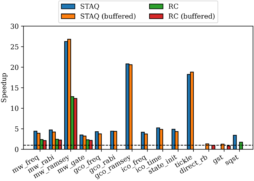
Figure 6: Kernel execution time speedup for our simulator relative to the execution time on a core device.

The results in Figure 6 show that simulation speeds up execution up to 26.8 times with an average speedup of 6.9 times. Especially the mw_ramsey, gco_ramsey, and tickle experiments achieve large speedups. The exceptional speedup for these experiments is caused by the long delays that are part of the experiment. The core device waits for these delays before the kernel finishes execution, while the simulator only simulates the passing of time but does not wait for it. The experiments that show the least speedup are the direct_rb and gst experiments. For STAQ, both experiments only yield a 1.3 times speedup, while for RC, the direct_rb experiment has no speedup and the gst experiment is slower with a speedup of 0.8 times. The limited speedup of these two experiments is caused by short delays and a high number of operations, which results in a high event density. As a result, the simulator must process many events while the experiment has a relatively short execution time on hardware. In general, we could state that the execution time on hardware $t_{\textit{hardware}}$ is mostly limited by the length of delays inserted during the experiment. These delays sum up to the total length of the timeline and therefore the duration of the experiment when running on hardware. The execution time of the simulator $t_{\textit{sim}}$ is not much affected by delays and instead is mostly limited by the total number of events present in the experiment. We know that speedup is defined as $S=t_{\textit{hardware}}/t_{\textit{sim}}$. Roughly speaking, we can derive that the total duration of an experiment is proportional to speedup while the total number of events is inversely proportional to speedup.

We can see from Figure 6 that the experiments running on the RC system always yield lower speedup compared to the same experiment running on STAQ. The different results are caused by differences in the control for the cooling and pumping procedures. Both procedures are executed by all experiments at the start of each sample. STAQ uses three digital outputs and one DDS while RC has additional features and uses five digital outputs and a DDS. As a result, RC inserts more events for each cooling and pumping procedure. Additionally, STAQ uses a constant DDS frequency for both procedures while RC uses a different frequency for each procedure which adds two additional DDS configuration events for each sample. Hence, the total number of events for RC experiments is higher than for STAQ which reduces the speedup. The additional DDS operations also insert extra delays into the experiment, but these delays do not compensate for the increased number of events. Figure 6 also shows buffered experiments tend to have slightly less speedup compared to their unbuffered counterparts. Buffering can reduce the execution time overhead of experiments resulting in faster execution on hardware. The total number of events per experiment is not affected by buffering. The result is a reduced speedup for experiments with buffering. The reduction in execution time by buffering is limited though due to the highly optimized control software.

In addition to speedup, we have also measured the timing accuracy of the simulated timeline cursor compared to execution on the core device. High timing accuracy is not a specific requirement for correct functional simulation, but a simulator with high timing accuracy could be used for estimating the timing of experiments. The timeline cursor simulation is accurate, but variable delays and inaccurate delays in simulated device drivers can still introduce errors. Variable delays mainly occur when the timeline cursor is synchronized with the RTIO counter. Such synchronization is performed at least once at the start of the experiment (see Section III-A) but can also occur at other moments. We simulate the synchronization of the timeline cursor using a timeline horizon and insert an additional delay of $125\times 10^{3}$ MU. We would like to emphasize that the presence of a variable delay indicates that the relative timing between the events before and after the delay is not relevant, and any variation will not negatively impact the functionality of the experiment or the simulation. Hence, simulating timeline cursor synchronization with a timeline horizon is sufficient for correct functional simulation. A variable delay can also occur when an experiment needs to wait for an input event that occurs at an unpredictable time, though none of the experiments in Table I contain such constructions. Inaccurate delays in simulated device drivers are often caused by a simplified timing model of the device driver. In practically all cases with inaccuracy, the simulated driver inserts less delay than the actual driver.

To measure the timing accuracy of the simulated timeline cursor, we store the value of the timeline cursor after the first synchronization with the RTIO counter and at the end of the experiment. The difference between the two values represents the total length of the event timeline in MU. We run the simulations with two configurations: regular and optimistic. When the timeline cursor is synchronized with the RTIO counter, our simulator inserts a fixed delay of $125\times 10^{3}$ and $0$ MU for the regular and optimistic configuration, respectively. We measured the event timeline length on the core device and with the two simulation configurations for all experiments listed in Table I using the STAQ and RC system. For each combination of system, experiment, and configuration, we calculate the relative error of the simulation which is defined as $(t_{\textit{sim}}-t_{\textit{exe}})/t_{\textit{exe}}$ where $t_{\textit{exe}}$ and $t_{\textit{sim}}$ are the measured event timeline lengths on the core device and during simulation, respectively. The results for are shown in Figure 7 and are also listed in Table II and III.

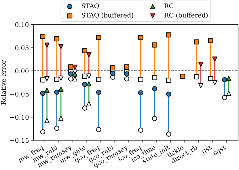
Figure 7: The error of the simulated timeline cursor relative to the timeline cursor of the core device. The filled markers represent the regular configuration while empty markers represent the optimistic configuration.

Experiment	STAQ		STAQ (buffered)
	Regular	Optimistic	Regular	Optimistic
mw_freq	-4.9%	-13.2%	7.4%	-2.0%
mw_rabi	-4.6%	-12.4%	6.9%	-1.8%
mw_ramsey	-0.7%	-1.8%	0.9%	-0.2%
mw_gate	-2.9%	-8.0%	4.4%	-1.2%
gco_freq	-4.6%	-12.7%	7.2%	-1.9%
gco_rabi	-0.5%	-1.4%	0.6%	-0.2%
gco_ramsey	-0.7%	-1.7%	0.9%	-0.2%
ico_freq	-4.8%	-12.8%	7.2%	-1.9%
ico_time	-3.9%	-10.3%	5.6%	-1.5%
state_init	-5.0%	-13.7%	7.8%	-2.0%
tickle	-1.2%	-1.3%	-1.2%	-1.3%
direct_rb			6.2%	-1.3%
gst			6.5%	-1.7%
sqst	-1.9%	-5.8%

TABLE II: The error of the simulated timeline cursor relative to the timeline cursor of the core device for STAQ.

Experiment	RC		RC (buffered)
	Regular	Optimistic	Regular	Optimistic
mw_freq	-4.2%	-10.8%	5.6%	-1.7%
mw_rabi	-4.0%	-10.2%	5.3%	-1.6%
mw_ramsey	-0.7%	-1.7%	0.8%	-0.3%
mw_gate	-2.8%	-7.1%	3.5%	-1.1%
direct_rb			1.4%	-3.2%
gst			2.5%	-2.6%
sqst	-1.6%	-4.9%

TABLE III: The error of the simulated timeline cursor relative to the timeline cursor of the core device for RC.

The results in Figure 7 show the error of the simulated timeline cursor relative to the timeline cursor of the core device. The regular and optimistic configurations are represented by the filled and empty markers, respectively. When comparing the results of the two different configurations, we see that the optimistic configuration always estimates a shorter timeline length, which is expected. If we only look at the results for the optimistic configuration, we see that all have a relative error lower or equal to 0.0. The optimistic configuration represents the lower-bound execution time where variable delays are always zero. When running on actual hardware, variable delays are not always zero, and as a result, the optimistic configuration underestimates the timeline length. We also noticed that all unbuffered results with regular configuration have a relative error lower or equal to 0.0. When running on hardware without buffers, the system has negative slack after each sample, and timeline synchronizations will insert delays larger than $125\times 10^{3}$ MU. The regular configuration underestimates the length of the variable delay and therefore underestimates the total timeline length. Regardless, the estimation of the regular configuration is better than that of the optimistic configuration for unbuffered experiments. The opposite is true for buffered experiments. Buffering reduces the length of variable delays caused by timeline synchronizations by maintaining slack between samples. The regular configuration is often too pessimistic for buffered experiments and the estimation of the optimistic configuration is better most of the time.

We noticed two other trends in Figure 7 that relate to the total timeline length of experiments. First, the results of some experiments have little spread, in particular mw_ramsey, gco_rabi, gco_ramsey, and tickle. These are all calibration experiments with relatively long delays and long total timeline lengths. The long timeline length combined with the limited sources of errors (i.e. low density of variable delays and events) results in a small relative error and therefore, a small spread between different configurations. Second, the results of the RC system tend to be closer to 0.0 than the equivalent STAQ results. We already mentioned that due to differences in the cooling and pumping procedures, the RC system inserts more events for each sample of the experiment. These additional events also insert extra delays into the experiment. As a result, the total timeline length of RC experiments are on average 28.1% longer compared to their STAQ equivalents. Again, the increased timeline length with no additional sources of errors reduces the relative error.

Overall, the average relative error for the regular configuration is 3.6%, and for the optimistic configuration, the average relative error is 4.4%. Based on our analysis of the regular and optimistic configurations, we concluded that the timeline length of buffered and unbuffered experiments are better estimated by the regular and optimistic configurations, respectively. When choosing the optimistic configuration for buffered experiments and the regular configuration for unbuffered experiments, the resulting average relative error is reduced to 2.1%, leading to an average accuracy of 97.9%. We can conclude that even in the presence of variable delays and simulated device drivers with simplified timing models, the position of the timeline cursor is simulated with high accuracy when choosing the appropriate configuration.

VI Conclusion

We have presented a functional simulation platform for real-time control software that enables software testing and verification. To simplify testing and verification, timeline manipulations and device drivers are simulated on the API level. Our simulation platform accurately simulates a timeline cursor using a stack while the event timeline is simulated using signals and events. Input signals are also simulated on a functional level and use the same interactive signal and event infrastructure used for output signals. We implemented a simulator based on the proposed concepts, which is part of our open-source library DAX. Our simulator integrates tightly into the ARTIQ environment and is capable of simulating real-time kernels and host-kernel interactions. We integrated our simulator with the standard Python unit test frameworks such that real-time control software can be tested using existing tools for step debugging, unit testing, and continuous integration. Compared to kernel execution on the core device, kernel simulation is 6.9 times faster on average. Even with the presence of variable delays and simplified timing models for device drivers, the position of the timeline cursor is simulated with an average accuracy of 97.9% when choosing the appropriate configuration.

References

- [1] Frank Arute et al. “Quantum supremacy using a programmable superconducting processor” In Nature 574.7779, 2019, pp. 505–510 DOI: 10.1038/s41586-019-1666-5
- [2] C. Ryan-Anderson et al. “Realization of Real-Time Fault-Tolerant Quantum Error Correction” In Phys. Rev. X 11 American Physical Society, 2021, pp. 041058 DOI: 10.1103/PhysRevX.11.041058
- [3] Lukas Postler et al. “Demonstration of fault-tolerant universal quantum gate operations” arXiv, 2021 DOI: 10.48550/ARXIV.2111.12654
- [4] Yuanhao Wang, Ying Li, Zhang-qi Yin and Bei Zeng “16-qubit IBM universal quantum computer can be fully entangled” In npj Quantum information 4.1 Nature Publishing Group, 2018, pp. 1–6
- [5] I. Pogorelov et al. “Compact Ion-Trap Quantum Computing Demonstrator” In PRX Quantum 2 American Physical Society, 2021, pp. 020343 DOI: 10.1103/PRXQuantum.2.020343
- [6] Rajeev Acharya et al. “Suppressing quantum errors by scaling a surface code logical qubit” arXiv, 2022 DOI: 10.48550/ARXIV.2207.06431
- [7] Guido Pagano et al. “A Quantum Approximate Optimization Algorithm in a Trapped-Ion Quantum Simulator” Proceedings of the National Academy of Sciences of the United States of America, 2020 URL: https://tsapps.nist.gov/publication/get_pdf.cfm?pub_id=928237
- [8] Junki Kim et al. “Hardware design of a trapped-ion quantum computer for Software-Tailored Architecture for Quantum co-design (STAQ) project” In Quantum 2.0, 2020, pp. QM6A–2 Optical Society of America
- [9] MS Blok et al. “Quantum information scrambling in a superconducting qutrit processor” In arXiv preprint arXiv:2003.03307, 2020
- [10] Sébastien Bourdeauducq et al. “ARTIQ 1.0” Zenodo, 2016 DOI: 10.5281/zenodo.51303
- [11] Vlad Negnevitsky “Feedback-stabilised quantum states in a mixed-species ion system”, 2018
- [12] Peter Maunz, Jonathan Mizrahi and Josh Goldberg “IonControl v. 1.0, Version 00”, 2016 URL: https://www.osti.gov/biblio/1326630
- [13] X. Fu et al. “eQASM: An Executable Quantum Instruction Set Architecture” In 2019 IEEE International Symposium on High Performance Computer Architecture (HPCA), 2019, pp. 224–237 DOI: 10.1109/HPCA.2019.00040
- [14] Colm A Ryan et al. “Hardware for dynamic quantum computing” In Review of Scientific Instruments 88.10 AIP Publishing LLC, 2017, pp. 104703
- [15] Grzegorz Kasprowicz et al. “ARTIQ and Sinara: Open Software and Hardware Stacks for Quantum Physics” In OSA Quantum 2.0 Conference Optical Society of America, 2020, pp. QTu8B.14 DOI: 10.1364/QUANTUM.2020.QTu8B.14
- [16] J.A. Rowson “Hardware/Software Co-Simulation” In 31st Design Automation Conference, 1994, pp. 439–440 DOI: 10.1109/DAC.1994.204143
- [17] Ken Hines and Gaetano Borriello “Dynamic Communication Models in Embedded System Co-Simulation” In Proceedings of the 34th Annual Design Automation Conference, DAC ’97 Anaheim, California, USA: Association for Computing Machinery, 1997, pp. 395–400 DOI: 10.1145/266021.266178
- [18] Jason Lowe-Power et al. “The gem5 Simulator: Version 20.0+” arXiv, 2020 DOI: 10.48550/ARXIV.2007.03152
- [19] Preeti Ranjan Panda “SystemC: A Modeling Platform Supporting Multiple Design Abstractions” In Proceedings of the 14th International Symposium on Systems Synthesis, ISSS ’01 Montréal, P.Q., Canada: Association for Computing Machinery, 2001, pp. 75–80 DOI: 10.1145/500001.500018
- [20] “IEEE Standard for Standard SystemC Language Reference Manual” In IEEE Std 1666-2011 (Revision of IEEE Std 1666-2005), 2012, pp. 1–638 DOI: 10.1109/IEEESTD.2012.6134619
- [21] Jonathan Bachrach et al. “Chisel: Constructing hardware in a Scala embedded language” In DAC Design Automation Conference 2012, 2012, pp. 1212–1221 DOI: 10.1145/2228360.2228584
- [22] Claude Helmstetter and Vania Joloboff “SimSoC: A SystemC TLM integrated ISS for full system simulation” In APCCAS 2008 - 2008 IEEE Asia Pacific Conference on Circuits and Systems, 2008, pp. 1759–1762 DOI: 10.1109/APCCAS.2008.4746381
- [23] Cagkan Erbas, Andy D. Pimentel, Mark Thompson and Simon Polstra “A Framework for System-Level Modeling and Simulation of Embedded Systems Architectures” In EURASIP Journal on Embedded Systems 2007.1, 2007, pp. 082123 DOI: 10.1155/2007/82123
- [24] A.D. Pimentel, C. Erbas and S. Polstra “A systematic approach to exploring embedded system architectures at multiple abstraction levels” In IEEE Transactions on Computers 55.2, 2006, pp. 99–112 DOI: 10.1109/TC.2006.16
- [25] Gushu Li, Yufei Ding and Yuan Xie “Sanq: A simulation framework for architecting noisy intermediate-scale quantum computing system” In arXiv preprint arXiv:1904.11590, 2019
- [26] Xiang Fu et al. “Quingo: A Programming Framework for Heterogeneous Quantum-Classical Computing with NISQ Features” In arXiv preprint arXiv:2009.01686, 2020
- [27] L. Riesebos et al. “Pauli Frames for Quantum Computer Architectures” In Proceedings of the 54th Annual Design Automation Conference 2017, DAC ’17 Austin, TX, USA: Association for Computing Machinery, 2017 DOI: 10.1145/3061639.3062300
- [28] Leon Riesebos et al. “Quantum Accelerated Computer Architectures” In 2019 IEEE International Symposium on Circuits and Systems (ISCAS), 2019, pp. 1–4 DOI: 10.1109/ISCAS.2019.8702488
- [29] Krysta M Svore et al. “Q#: Enabling scalable quantum computing and development with a high-level domain-specific language” In arXiv preprint arXiv:1803.00652, 2018
- [30] Thien Nguyen et al. “Extending C++ for Heterogeneous Quantum-Classical Computing” In arXiv preprint arXiv:2010.03935, 2020
- [31] Robert S Smith, Michael J Curtis and William J Zeng “A practical quantum instruction set architecture” In arXiv preprint arXiv:1608.03355, 2016
- [32] Frederic T Chong, Diana Franklin and Margaret Martonosi “Programming languages and compiler design for realistic quantum hardware” In Nature 549.7671 Nature Publishing Group, 2017, pp. 180–187
- [33] John E Stone, David Gohara and Guochun Shi “OpenCL: A parallel programming standard for heterogeneous computing systems” In Computing in science & engineering 12.3 NIH Public Access, 2010, pp. 66
- [34] X. Fu et al. “An Experimental Microarchitecture for a Superconducting Quantum Processor” In Proceedings of the 50th Annual IEEE/ACM International Symposium on Microarchitecture, MICRO-50 ’17 Cambridge, Massachusetts: Association for Computing Machinery, 2017, pp. 813–825 DOI: 10.1145/3123939.3123952
- [35] Leon Riesebos, Brad Bondurant and Kenneth R Brown “Duke ARTIQ extensions (DAX)”, 2021 URL: https://gitlab.com/duke-artiq/dax
- [36] Leon Riesebos “Flake8 ARTIQ plugin”, 2020 URL: https://gitlab.com/duke-artiq/flake8-artiq
- [37] Ye Wang et al. “High-Fidelity Two-Qubit Gates Using a Microelectromechanical-System-Based Beam Steering System for Individual Qubit Addressing” In Phys. Rev. Lett. 125 American Physical Society, 2020, pp. 150505 DOI: 10.1103/PhysRevLett.125.150505
- [38] “Xilinx KC705” URL: https://www.xilinx.com/products/boards-and-kits/ek-k7-kc705-g.html
- [39] Easwar Magesan, Jay M Gambetta and Joseph Emerson “Scalable and robust randomized benchmarking of quantum processes” In Physical review letters 106.18 APS, 2011, pp. 180504
- [40] Timothy J. Proctor et al. “Direct Randomized Benchmarking for Multiqubit Devices” In Phys. Rev. Lett. 123 American Physical Society, 2019, pp. 030503 DOI: 10.1103/PhysRevLett.123.030503
- [41] Jeffrey M Epstein, Andrew W Cross, Easwar Magesan and Jay M Gambetta “Investigating the limits of randomized benchmarking protocols” In Physical Review A 89.6 APS, 2014, pp. 062321
- [42] Robin Blume-Kohout et al. “Robust, self-consistent, closed-form tomography of quantum logic gates on a trapped ion qubit” arXiv, 2013 DOI: 10.48550/ARXIV.1310.4492
- [43] Roman Schmied “Quantum state tomography of a single qubit: comparison of methods” In Journal of Modern Optics 63.18 Taylor & Francis, 2016, pp. 1744–1758
- [44] Leon Riesebos et al. “Modular software for real-time quantum control systems” In 2022 IEEE International Conference on Quantum Computing and Engineering (QCE), 2022
- [45] “Duke ARTIQ extensions (DAX) zoo”, 2022 URL: https://gitlab.com/duke-artiq/dax-zoo