Arc travel time and path choice model estimation subsumed

Abstract

We propose a method for maximum likelihood estimation of path choice model parameters and arc travel time using data of different levels of granularity. Hitherto these two tasks have been tackled separately under strong assumptions. Using a small example, we illustrate that this can lead to biased results. Results on both real (New York yellow cab) and simulated data show strong performance of our method compared to existing baselines.

1 Introduction

An extensive literature on traffic-related problems aims at decreasing congestion through improved strategic and tactical planning as well as real-time traffic management. Central to many of these problems is, on the one hand, the problem of estimating travel times in a network and, on the other hand, the problem of predicting traffic flow. As we discuss in the following, these two problems are intrinsically connected and both require traffic data. However, they have been tackled separately in the literature under strong assumptions.

Consider a network of nodes and arcs representing a given congested geographical area. Estimating the travel times between any origin and destination node pair in this network is difficult because it depends on numerous factors such as speed limit, traffic flow, road capacity, accidents, construction work, traffic light states, etc. Some factors are easy to observe (e.g., speed limit), whereas others are not (e.g., state of traffic lights and accidents). Even if the factors are observable, the sources of data are diverse, for example, fixed sensors and floating car data. Travel time estimation methods are often tailor-made to the specificity of available data sources.

As pointed out in Bertsimas et al. (2019), for strategic and tactical planning purposes (e.g., routing and network design), it is more useful to estimate arc travel times as opposed to origin-destination (OD) travel times. Assuming that travelers follow a shortest path, Bertsimas et al. (2019) propose a methodology to estimate arc travel time by only observing the network and trip travel time between different OD pairs. Neatly, they do not need to observe the paths taken, nor the data on the demand structure (total demand between OD pairs).

The assumption that travelers follow paths minimizing travel time is strong in light of numerous empirical studies in the literature on route choice modeling (see Frejinger and Zimmermann, 2021, for a survey). In general, travelers do not follow the shortest paths with respect to some perfectly known generalized cost function. This motivates the use of stochastic prediction models where discrete choice (random utility maximization) models are the most widely used ones. Moreover, there is a related extensive literature on stochastic user equilibrium models (e.g., Dial, 1971, Fisk, 1980, Baillon and Cominetti, 2008). Noteworthy and complementary to the latter is the mean-risk traffic assignment model proposed by (Nikolova and Stier-Moses, 2014) based on the assumption that travel times (as opposed to the choice model) are stochastic and travelers minimize the expected travel time plus a multiple of the standard deviation of travel time (a stochastic shortest path problem). To summarize, methods in the aforementioned literature are based on the assumption that travelers do not follow (deterministic) shortest paths. Either because the analyst, or the travelers, do not perfectly observe relevant network attributes, such as travel time.

Discrete choice models are widely used to predict traffic flow. They are central to variety of problems where the purpose is to predict flow in response to changes in network attributes, such as travel time, or its structure (e.g., network design or facility location problems). Two data sources are required to estimate values of related unknown parameters: First, a representation of the network in question, including attributes such as arc travel times. With relatively few exceptions (e.g., Gao et al., 2010, Ding-Mastera et al., 2019, Mai et al., 2021), the attributes are assumed to be deterministic. Second, path choice observations. Most commonly, model parameters are estimated by maximum likelihood using path observations. The estimation is done assuming that network attributes are exogenously given. The latter assumption stands in contrast with the literature on travel time estimation and equilibrium models. It is a strong assumption as the data generation process (by the travelers) is the same as, for example, Bertsimas et al. (2019) even if the required level of detail is higher (path observations as opposed to only path travel time).

The objective of this work is to relax the assumption that travel times are exogenous when estimating path choice models. In addition, we aim to design a maximum likelihood estimator for travel time estimation that is based data assumptions similar to Bertsimas et al. (2019) but with weaker assumptions on the path choice model.

We provide the following contributions:

• We propose a methodology to simultaneously estimate arc travel times and parameters of differentiable path choice models. We show that under weak assumptions we can conveniently formulate a maximum likelihood estimator for the seemingly more complex joint estimation problem. Furthermore, we show that under the assumptions made by Bertsimas et al. (2019), their method is, in fact, corresponds to maximum likelihood estimation.

• An attractive property of our proposed joint likelihood is that it allows naturally to mix observations of different levels of granularity.

• We show through an illustrative example that treating travel time as exogenous variables can lead to biased results.

• Numerical results based on New York City taxi data show that estimating a maximum likelihood estimation of the joint likelihood is fast and performant. Measured by root mean-squared log error, we reach a performance and computing times comparable to those of Bertsimas et al. (2019) while solving the joint estimation problem. Results on synthetic data illustrate that our travel time estimates better reproduce ground truth ones and achieves better path choice model parameter estimates than a sequential approach (first estimating arc travel times, followed by the choice model).

The remainder of the paper is structured as follows. In Section 2, we describe the work of Bertsimas et al. (2019), and the arc-based path choice model of Fosgerau et al. (2013) that we use in our our experiments. In Section 3 we provide an illustrative example, and in Section 4 we introduce our method. We report numerical experiments in Section 5, and finally, we provide concluding remarks in Section 6.

2 Related work

Our work is situated at the intersection between the literature on arc travel time estimation and path choice model estimation. A comprehensive literature review on these two topics is out of the scope of this paper. Instead, we focus this section on the most closely related works and refer to Mori et al. (2015) or Oh et al. (2015) for broader reviews on travel time estimation and refer to Prato (2009), Frejinger and Zimmermann (2021), and Zimmermann and Frejinger (2020) for broader reviews concerning path choice models. First, we briefly outline the method of Bertsimas et al. (2019) that we base our work on. Second, in Section 2.2, we describe recursive path choice models (Zimmermann and Frejinger, 2020) that allow for maximum likelihood estimation of unknown parameters based on trajectory observations. Finally, in Section 2.3 we discuss contrasts and synergies between these works.

2.1 A method for arc travel time estimation

Given a graph $G=(N,A)$ where $N$ is the set of nodes and $A$ the set of arcs, let $O$ be multi-set (i.e., a set with the possibility of duplicate elements) of observations $(o,d,t)\in N^{2}\times\mathbb{R}_{+}$ from trajectories in $G$ such that $o$ is the origin, $d$ is the destination, and $t$ is the travel time. Bertsimas et al. (2019) focus on estimating the travel time of $a\in A$ using $O$.

Based on the assumption that the quality of travel time estimations is perceived on a multiplicative rather than an additive scale, Bertsimas et al. (2019) propose using the mean-squared log error (MSLE),

$$\mathrm{MSLE}(\hat{t},t)=(\ln t-\ln\hat{t})^{2}=\ln^{2}(t/\hat{t}),$$ (1)

as a loss function to compare estimate $\hat{t}$ and the observed $t$. Furthermore, they propose the convex surrogate,

$$\max\left\{\frac{\hat{t}}{t},\frac{t}{\hat{t}}\right\},$$ (2)

for $\mathrm{MSLE}(\hat{t},t)$ which they model using a second order cone and a linear constraint.

Bertsimas et al. (2019) formulate the estimation problem as a mixed-integer program whose objective is to minimize MSLE between travel times of shortest paths (i.e., predicted travel times) and observed travel times. We refer to this mixed-integer program as BDJM model (from the first letter of each contributing author’s name). The objective also has a regularization term which we describe in more detail below. The BDJM model has two sets of variables: Binary variables to select the shortest path between each OD pair and a set of continuous variables corresponding to arc and path travel times. Linear (including big-M) constraints ensure that, for each OD pair, the travel time of the shortest path is the sum of its arc travel times and is shorter than all other paths.

The regularization term plays an important role in this formulation. Bertsimas et al. (2019) define the regularization for the 3-tuple $(i,j,k)$ such that $(i,j)$ and $(j,k)$ are arcs as

$$\left|\frac{\boldsymbol{T}_{ij}}{\boldsymbol{L}_{ij}}-\frac{\boldsymbol{T}_{jk}}{\boldsymbol{L}_{jk}}\right|\frac{2}{\boldsymbol{L}_{ij}+\boldsymbol{L}_{jk}},$$ (3)

where $\boldsymbol{T}_{ij}$ and $\boldsymbol{L}_{ij}$ are, respectively, the length and the travel time of the arc $(i,j)\in A$. The regularization for the whole problem is the sum of the regularization for all 3-tuples like $(i,j,k)$. This term introduces a notion of smooth solutions, which helps to navigate the undetermined solution space, obtain more realistic solutions, and mitigate the risk of overfitting.

Since this program is hard to solve, they first relax some of the constraints related to the shortest paths and use a decomposition scheme where they iteratively solve the program on the real and binary variables until convergence. We call this the BDJM method.

Bertsimas et al. (2019) evaluate their method on New York city’s yellow cab dataset (New York City Taxi and Limousine Commission, 2016) limited to Manhattan and obtain high-quality results. Solving the problem is challenging due to the large network and the many observations.

2.2 Path choice models

A path choice model is a mathematical object that takes the arc travel time $\boldsymbol{T}$, a parameter vector $\boldsymbol{b}$, and other exogenous attributes as inputs. Path choice models can be used to sample paths conditioned on an OD pair, or to compute traffic flow between OD pairs. Furthermore, path choice models can estimate the probability of sampling any path. We call a path choice model differentiable if the probability of sampling any path is differentiable with regards to the path choice model’s inputs. This point of view helps us to reason about most work that deals with modeling path choice preferences. It is possible to model path choices as a Markov Decision Process (MDP), in that case we call it a recursive path choice model.

The recursive logit – a recursive path choice model – was introduced in Fosgerau et al. (2013) with the objective to analyze and predict travelers’ path choices. They show that the multinomial logit (MNL) of McFadden (1977) on the set of all paths can be formulated as a parametric MDP. The MDP structure allows parameter estimation without defining a set of alternative paths. More recent studies propose models that relax the restrictive assumptions of the MNL model. We refer to Zimmermann and Frejinger (2020) and Frejinger and Zimmermann (2021) for overviews.

The MDP proposed by Fosgerau et al. (2013) has similarities with the work of Ziebart et al. (2008) in the inverse reinforcement learning community. The main difference between these two work is that while conditioned on OD, the ratio of probability for any two path is the same, Fosgerau et al. (2013) proposes an MDP with only negative rewards and an absorbing state while Ziebart et al. (2008)’s model has no absorbing state. Furthermore, Fosgerau et al. (2013) proposes to solve a system of linear equations instead of doing value iteration and conditions the MDP on the destination. We focus this section on the recursive logit model as we use it to illustrate our method.

Like McFadden (1977), Fosgerau et al. (2013) assume that people are rational in the sense that they choose the path that maximizes a utility function. Let $u(r)$ be the utility of selecting a path $r$; the probability of someone choosing $r$ over the set of all paths from $o$ to $d$, $R(o,d)$, is

$$\mathbb{P}(r)=\mathbb{P}(u(r)>u(s)|\forall s\neq r\in R(o,d)).$$ (4)

Since people have different preferences, they model it as the sum of a deterministic term $v(r)$ and a random variable $\varepsilon(r)$. The random variable models personal differences, the unknown to the analyst, the ever-changing environmental factors, and the alignment of stars.

Fosgerau et al. (2013) assume that both deterministic and stochastic parts are arc-additive and that state transitions are deterministic. This way, the deterministic component of the utility $v(r)$ can be written as the sum of arc utilities, i.e., $\sum_{(i,j)\in r}v(j|i)$ where $v(j|i)$ is the utility of traversing an arc $(i,j)$ and $(i,j)\in r$ represent all traversed arcs in $r$. The stochastic term $\varepsilon(r)$ is also the sum of per arc stochasticity i.e., $\sum_{(i,j)\in r}\varepsilon(j|i)$. They assume that $\varepsilon(j|i)$ are independent and identically distributed (i.i.d.) random variables following the Extreme Value type I distribution like in McFadden (1977) and are independent of all known information. Given said hypothesis, the probability of choosing a path $r$ among all paths with the same OD is given by the MNL as

$$\mathbb{P}(r|o,d)=\dfrac{\exp[v(r)]}{\sum_{s\in R(o,d)}\exp[v(s)]}.$$ (5)

For a given destination $d$, let $w(i;d)$ be the expected maximum utility when going from a node $i$ to the destination $d$. It is given by the Bellman equation (Bellman, 1954)

$$w(i;d)=\mathbb{E}[\max_{j\in N(i)}u(j|i)+w(j;d)],$$ (6)

where $N(i)$ is the set of all outgoing neighbors of $i$ i.e., $N(i)=\{j\in N|(i,j)\in A\}$. The solution to (6) is given by the so-called logsum

$$w(i;d)=\begin{cases}\ln\sum_{j\in N(i)}\exp[v(j|i)+w(j;d)]&\text{if $a\neq d$},\\ 0&\text{otherwise.}\end{cases}$$ (7)

The probability of choosing any neighboring node $j$ is given by the MNL model as

$$\mathbb{P}(j|i;d)=\frac{\exp[v(j|i)+w(j;d)]}{\sum_{k\in N(i)}\exp[v(k|i)+w(k;d)]}.$$ (8)

It is important to note that whereas the utilities are stochastic, the state transitions are not (for a given state and action, the next state is deterministic). This assumption allows fast estimation, as shown in Appendix A.

Fosgerau et al. (2013) estimate parameters by maximizing the likelihood of observed trajectories. For this purpose, they use the nested fixed-point algorithm Rust (1987, 1988). They decompose the problem into an outer and an inner problem. The latter consists in finding the path probabilities given the value function. The former corresponds to finding the parameters that maximize the log-likelihood of the path probabilities. Let $Y$ be a set of observed paths, the log-likelihood or the “outer” loss is

$$\max_{\hat{\boldsymbol{b}}}\mathbb{E}[\ln\mathbb{P}(r;\hat{\boldsymbol{b}})]\approx\min_{\hat{\boldsymbol{b}}}-\frac{1}{|Y|}\sum_{r\in Y}\ln\mathbb{P}(r;\hat{\boldsymbol{b}}),$$ (9)

where $\hat{\boldsymbol{b}}$ a vector of choice model parameters.

2.3 Contrasts and synergies

In this section, we highlight contrasts and synergies between BDJM method and path choice models (in particular Fosgerau et al., 2013).

First we note that the solution approaches are radically different. The model of Fosgerau et al. (2013) is differentiable, and they use gradient methods. On the contrary, the lack of gradients is a source of complexity in the BDJM method.

Both works make assumptions about travelers’ path choices: the BDJM model assume that they choose the shortest path with regards to the estimated arc travel time matrix whereas Fosgerau et al. (2013) relax this assumption by modeling arc utilities as random and account for different behaviors.

Regarding data, the method of Bertsimas et al. (2019) only requires observations of OD travel times. It could be extended to use trajectory observations (with some changes, as the original program might be infeasible). In contrast, estimating path choice models requires this detailed type of data. In addition, travel time information is assumed to be available and treated as exogenous. The use of aggregate data (such as OD travel times) has important advantages. First, trajectory data can be costly to collect, and the mapping to a graph representation of the network is challenging (Quddus and Washington, 2015, Chen et al., 2014). Second, detailed data may puts the privacy of travelers at risk.

In summary, following the state-of-the-art, a two-step procedure is required to estimate path choice models. First, we estimate arc travel times. Second, we use arc travel times as exogenous attributes when estimating parameters of a path choice model. The first step can be as simple as computing free-flow travel times, or as sophisticated as the approach proposed by Bertsimas et al. (2019).

The estimated path choice models – i.e., the result of step two – have different applications. For example, the parameters can be used to analyze value of time (e.g., Fosgerau and Karlström, 2010). The model can be used to predict traffic flow for network optimization or for solving an equilibrium model. In this context, the aforementioned two-step approach is adequate if, under conditions similar to the observations, the travel times resulting from predicted traffic flows (application of estimated path choice model) are close to the estimated travel times (result of step one). Next, we describe a small example illustrating that this is not necessarily true, hence motivating the need to consider the two steps jointly.

3 Two arcs, one hard network

Figure 1: A two-arc network. Arc travel times, $t_{1}$ and $t_{2}$, are given next to each arc.

The motivation behind our work is the interdependence between the problems of estimating arc travel times and path choice model parameters: Arc travel times are needed to estimate the path choice model, and a path choice model to estimate the arc travel times. Instead of viewing these as two sequential steps, as a thought experiment let us imagine an iterative scheme that switches between these tasks. With a small example (see Figure 1), we show that if we start with a reasonable starting point and switch between estimating either the transition probability or a better travel time estimate, the process will either diverge or converge to sub-optimal solutions.

In the following, we assume that the probability of choosing the upper arc in Figure 1 is

$$p=\mathbb{P}(C=1)=\frac{\exp(-x)}{\exp(-x)+\exp(-1)}.$$ (10)

Furthermore, we use the MSLE to compare our estimate and the observation; we minimize the loss by changing the travel time of arc 1, that is, $x$ in the graph shown in Figure 1. The travel time of arc 2 is assumed to be 1 time unit. We have observed that a user has gone from the node $o$ to the node $d$, and it took them 2 time units. Our only unknown is $x$, and its starting value is 1 time unit.

Loss of expected travel time.

In this example, minimizing the loss of the expected travel time will result in divergence. As the expected travel time needs to be greater than 1 to reduce the loss, $x$ has to increase. However, an increase in $x$ leads to a smaller $p$ and for smaller $p$ the optimal $x$ is larger. Thus $x$ will diverge as this feedback loop will not stop. We show this analytically. The expected travel time is $x\mathbb{P}(C=1)+\mathbb{P}(C=2)$ and the optimal $x$ (when the expected travel time is 2 time units) given $p$ is

$$\frac{2-1\mathbb{P}(C=2)}{\mathbb{P}(C=1)}=\frac{1+\mathbb{P}(C=1)}{\mathbb{P}(C=1)}=1+\frac{1}{\mathbb{P}(C=1)}=1+\frac{1}{p}.$$ (11)

Expected loss.

Minimizing the expected loss is more straightforward. The optimum of $x$, regardless of $p$, will be 2. When $x$ equals 2, the loss is approximately 0.35, but the loss at the optimum is around 0.32. The issue arises since the derivative of $p$ with respect to $x$ is not zero. The derivative of the loss $l(x,p)$ with respect to $x$ is

$$\nabla_{x}l(x,p(x))=\nabla_{1}l(x,p(x))+\nabla_{2}l(x,p(x))\nabla_{x}p(x)$$ (12)

but the iterative process assumes $\nabla_{x}p(x)$ is zero; this can lead to divergences or non-optimal solutions.

This illustrative example shows that even given a simple graph, it is possible to diverge or find sub-optimal solutions if arc travel times and path choice model estimations are done in a sequential fashion.

Whereas iterative schemes are not used in practice, an important implication of this simple example is that bias in travel time estimates may be absorbed by path choice model parameter estimates. See de Moraes Ramos et al. (2020) for an empirical investigation of this issue when they compare static and dynamic travel time sources.

4 Methodology

In this section, we introduce a mixture that models trips in the network. We analyze the properties of the mixture, and deliniate a solution approach. Whereas our methodology is different from both Bertsimas et al. (2019) and Fosgerau et al. (2013), we reuse the notation which pertains to the problem unless stated otherwise.

4.1 A mixture of distributions for flexible loss functions

For every trip in $G$, we represent it as a four-tuple

$$(o,d,t,r)\in N^{2}\times\mathbb{R}_{+}\times R(o,d),$$ (13)

where, like before, $o$ is the origin, $d$ is the destination, $t$ is a travel time observation, and $r$ is the path taken. We assume that they follow a mixture of distributions:

$$o\sim\mathcal{O},$$ (14a)

$$d\sim\mathcal{D}(o),$$ (14b)

$$r\sim\mathcal{P}(o,d;\boldsymbol{T},\boldsymbol{b}),$$ (14c)

$$\hat{t}=\sum_{(i,j)\in r}\boldsymbol{T}_{ij},$$ (14d)

$$t\sim\mathcal{N}(\hat{t}).$$ (14e)

Origin $o$ follows a distribution $\mathcal{O}$ over the set of all nodes, and $d$ follows a distribution $\mathcal{D}(o)$ over the set of all nodes except $o$. Path $r$ follows a distribution over the set of all paths $R(o,d)$ described by the path choice model $\mathcal{P}(o,d;\boldsymbol{T},\boldsymbol{b})$ that is parameterised by $\boldsymbol{b}$. To simplify the notation we omit explicitly defining other features as they are assumed to be fixed and exogenous. The path length $\hat{t}$ is the travel time of $r$. The observed travel time $t$ follows a distribution $\mathcal{N}$ parameterized by $\hat{t}$ with positive support, ideally $\mathbb{R}_{+}$ as some observations may otherwise have zero likelihood. It models the difference in travel time due to factors like fluctuating arc travel time, luck, non-optimal habits, and going over the speed limit. Given this mixture, we implicitly assume that observed trajectories are i.i.d. This is a standard assumption even if it typically does not hold as the next trip often originates from a previous destination.

Given our mixture, the likelihood of an observation $(o,d,t,r)$ is

$$f(o,d,r,t)=\mathbb{P}(o)\mathbb{P}(d|o)\mathbb{P}(r|o,d)f(t;\hat{t}),$$ (15)

where $f(t;\hat{t})$ is likelihood function of $t$ parameterized by $\hat{t}$. If we do not observe any of the elements, we marginalize it. For instance, if we do not observe the path for an observation $(o,d,t)$, the likelihood is

$$f(o,d,t) =\sum_{r\in R(o,d)}\mathbb{P}(o)\mathbb{P}(d|o)\mathbb{P}(r|o,d)f(t;\hat{t})$$ (16)

$$=\mathbb{P}(o)\mathbb{P}(d|o)\mathbb{E}_{r\sim\mathcal{P}}\left[f(t;\hat{t})\right],$$ (17)

where $\mathcal{P}$ is shorthand for $\mathcal{P}(o,d;\boldsymbol{T},\boldsymbol{b})$. The corresponding log-likelihood is

$$\ln f(o,d,t)=\\ \ln\mathbb{P}(o)+\ln\mathbb{P}(d|o)+\ln\mathbb{E}_{r\sim\mathcal{P}}\left[f(t;\hat{t})\right].$$ (18)

Similarly, if we do not observe the travel time, we obtain

$$f(o,d,r) =\int_{0}^{\infty}f(o,d,r,t)\mathrm{d}t$$ (19)

$$=\int_{0}^{\infty}\mathbb{P}(o)\mathbb{P}(d|o)\mathbb{P}(r|o,d)f(t;\hat{t})\mathrm{d}t$$ (20)

$$=\mathbb{P}(o)\mathbb{P}(d|o)\mathbb{P}(r|o,d)\int_{0}^{\infty}f(t;\hat{t})\mathrm{d}t$$ (21)

$$=\mathbb{P}(o)\mathbb{P}(d|o)\mathbb{P}(r|o,d).$$ (22)

The equality holds because probability density functions (pdf) have unit integral. As such

$$\ln f(o,d,p)=\ln\mathbb{P}(o)+\ln\mathbb{P}(d|o)+\ln\mathbb{P}(r|o,d).$$ (23)

When we are only estimating the path choice model and assume that travel times are exogenous, the log-likelihood (23) corresponds to the log-likelihood commonly used for estimating path choice models, like (9).

We can also find a distribution over the destinations if we only observe the origin and the travel time. The probability that the destination of an observation $(o,t)$ is $d$ is

$$\mathbb{P}(d|o,t)=\mathbb{P}(o,d,t)/\mathbb{P}(o,t).$$ (24)

The term $\mathbb{P}(o,t)$ is a normalization term as it is constant with regard to the the integral variable regardless of the destination so we compare the probability $\mathbb{P}(o,d,t)$ over all possible destinations.

It is also possible to combine different log-likelihoods. For example, for an observation $(o_{1},d_{1},t_{1})$ and an observation $(o_{2},d_{2},r_{2},t_{2})$, the total log-likelihood is

$$\ln f(o_{1},d_{1},t_{1})+\ln f(o_{2},d_{2},r_{2},t_{2}).$$ (25)

In other words, we have a formulation that can mix different types of data consistently. In contrast, an alternative adding weighted losses (one loss for each data type) would introduce hyper parameters to control the ratio of the losses.

Inspired by the literature of energy-based models (EBM) (LeCun et al., 2007), we can convert a large class of loss functions to distributions whose log-likelihood is the original loss function. However unlike the EBM literature we do not require the loss function to also be an energy function as we are not interested in EBMs.

Proposition 1.

For any function $L:\mathbb{D}\rightarrow\mathbb{R}$ and a parameter vector $\theta$, let

$$Z_{L}(\theta)=\int_{\mathbb{D}}\exp[-L(x,\theta)]\mathrm{d}x$$ (26)

be the partition function. Whenever $Z_{L}(\theta)$ converges,

$$f_{L}(x;\theta)=\begin{cases}\exp[-L(x,\theta)]/Z_{L}(\theta)&\text{if $x\in\mathbb{D}$}\\ 0&\text{otherwise,}\end{cases}$$ (27)

is a valid probability density function. Furthermore, if $Z_{L}$ is a constant independent of $\theta$, the log-likelihood of the distribution corresponding to $f_{L}$ is the original loss function.

Proof.

The first part is easy as to check. The density is necessarily positive as the exponent of any real number is positive. The integral of $f$ over all reals is equal to the integral over $\mathbb{D}$, we can then take out the partition function because it is constant and get the partition function divided by itself which is equal to one. The log-likelihood is $\log f_{L}(x;\theta)=-L(x,\theta)-\log Z_{L}(\theta)$ hence maximizing the log-likelihood is equivalent to minimizing the loss function if $Z_{L}$ is a constant. ∎

Remark 1.

There are many examples of such functions like the $\mathrm{MSE}(x,y)=(x-y)^{2}$ that corresponds to the normal distribution with $\sigma^{2}=0.5$ or the $\mathrm{LINEX}(x,y)=\exp(x-y)-(x-y)-1$ function that corresponds to the Gumbel distribution (Abdzaid Atiyah et al., 2020).

Remark 2.

Whereas from an optimization perspective multiplying by a number does not change the minimum of the problem, it changes the corresponding distribution.

Unfortunately, the partition function resulting from applying Proposition 1 to the MSLE is not constant. Therefore, we introduce what we call the small time biased MSLE (SMSLE)

$$\mathrm{SMSLE}_{\gamma}(t,\hat{t})=\gamma\mathrm{MSLE}(t,\hat{t})+\ln t,$$ (28)

Proposition 2.

The optimum of the optimization problem with SMSLE as loss function is the same as the problem with MSLE as loss function and the partition function of SMSLE is a constant.

Proof.

The first part is true due to the fact that $t$ is a constant in the optimization problem. The partition function is

$$Z_{\mathrm{SMSLE}}(\theta)=\int_{0}^{\infty}\exp[-\gamma(\ln x-\ln\theta)^{2}-\ln x]\mathrm{d}x.$$ (29)

Let $y=\ln x$, we can do a change of variable in the integral and get

$$\int_{-\infty}^{\infty}\exp[-\gamma(y-\ln\theta)^{2}-y]\exp(y)\mathrm{d}y.$$ (30)

This can be simplified to

$$\int_{-\infty}^{\infty}\exp[-\gamma(y-\ln\theta)^{2}]\mathrm{d}y.$$ (31)

Doing a second change of variable using $z=\sqrt{\gamma}(y-\ln\theta)$ results

$$\int_{-\infty}^{\infty}\exp[-z^{2}]\frac{1}{\sqrt{\gamma}}\mathrm{d}z.$$ (32)

It is well-known that that the limit of the error function at infinity or

$$2/\sqrt{\pi}\int_{0}^{\infty}\exp(-x^{2})\mathrm{d}x$$ (33)

is one. By symmetry (32) is equal to $\sqrt{\pi/\gamma}$. The function $f_{\mathrm{SMSLE}}$ corresponds to a log-normal with $\mu=\log(\theta)$ and $\sigma=1/\sqrt{2\gamma}$. ∎

Proposition 3.

The solution to the BDJM model is the maximum likelihood estimate of (14) where the path choice model is a shortest path algorithm and $\mathcal{O}$ and $\mathcal{D}(o)$ are not estimated.

Proof.

When $\mathcal{P}$ is a shortest path, the expectation in (18) is equal to $f(t;\hat{t})$ for the shortest path $r$. If we chose $\mathcal{N}$ to be the log normal, $\ln f(t;\hat{t})$ is proportional to the MSLE. As such, the BDJM method results in a maximum likelihood estimates. ∎

Whereas it might seem possible to address the interdependece issue using data that has both path and travel time information, it can lead to a biased estimator if the path choice model depends on the observed travel time.

Proposition 4.

Ignoring the link between travel time and path choice model when training a maximum likelihood estimator for the mixture can lead to a biased estimator.

Proof.

If the path choice model depends on the travel times, the maxima of (19) and (15) with regards to $\boldsymbol{T}$ can be different. ∎

Remark 3.

Proposition 4 implies that if the path choice model does not depend on travel times, it is possible to overcome the circular dependency by observing paths.

4.2 Solution approach

To compute maximum likelihood estimates, we need to maximize the likelihood of the observed data. To achieve this hereon now, we assume that the function $\ln\mathbb{P}(r\sim\mathcal{P})$ is differentiable with respect to the travel time and the path choice model’s parameters.

Assumption 1.

We assume that $\nabla_{\boldsymbol{b},\boldsymbol{T}}\ln\mathbb{P}(r)$ exists.

No statement before this one made any assumption on the differentiability but in order to estimate the model, we limit ourselves to differentiable models. While we illustrate our method using a recursive logit model, we are not limited to that class of path choice models.

In this section we focus on observation with no path because the treatment of other kind of observation are similar or easier. The gradient of the log-likelihood is

$$\nabla\ln f(o,d,t)=\nabla\ln\mathbb{P}(o)+\nabla\ln\mathbb{P}(d|o)+\nabla\ln\mathbb{E}_{r\sim\mathcal{P}}\left[f(t;\hat{t})\right].$$ (34)

Proposition 5.

We can estimate $\nabla\ln\mathbb{E}_{r\sim\mathcal{P}}\left[f(t;\hat{t})\right]$ in (34) using the offline estimator

$$\mathbb{E}_{r\sim\mathcal{P}^{\prime}}\left[\nabla f(t;\hat{t})+f(t;\hat{t})\frac{\nabla\mathbb{P}_{\mathcal{P}}(r)}{\mathbb{P}^{\prime}_{\mathcal{P}}(r)}\right]$$ (35)

and online estimator

$$\mathbb{E}_{r\sim\mathcal{P}}\left[\nabla f(t;\hat{t})+f(t;\hat{t})\nabla\ln\mathbb{P}_{\mathcal{P}}(r)\right],$$ (36)

for any distribution $\mathcal{P}^{\prime}$ whose support is a superset of the support of $\mathcal{P}$, i.e. such that $\mathcal{P}\ll\mathcal{P}^{\prime}$.

Proof.

We rewrite the gradient of the expected likelihood as

$$\nabla\mathbb{E}_{r\sim\mathcal{P}}\left[f(t;\hat{t})\right]$$ (37)

$$=\nabla\mathbb{E}_{r\sim\mathcal{P}^{\prime}}\left[f(t;\hat{t})\frac{\mathbb{P}_{\mathcal{P}}(r)}{\mathbb{P}_{\mathcal{P}^{\prime}}(r)}\right]$$ (38)

$$=\mathbb{E}_{r\sim\mathcal{P}^{\prime}}\left[\nabla f(t;\hat{t})\frac{\mathbb{P}_{\mathcal{P}}(r)}{\mathbb{P}_{\mathcal{P}^{\prime}}(r)}+f(t;\hat{t})\frac{\nabla\mathbb{P}_{\mathcal{P}}(r)}{\mathbb{P}_{\mathcal{P}^{\prime}}(r)}\right]$$ (39)

$$=\mathbb{E}_{r\sim\mathcal{P}}\left[\left(\nabla f(t;\hat{t})\frac{\mathbb{P}_{\mathcal{P}}(r)}{\mathbb{P}_{\mathcal{P}^{\prime}}(r)}+f(t;\hat{t})\frac{\nabla\mathbb{P}_{\mathcal{P}}(r)}{\mathbb{P}_{\mathcal{P}^{\prime}}(r)}\right)\frac{\mathbb{P}_{\mathcal{P}^{\prime}}(r)}{\mathbb{P}_{\mathcal{P}}(r)}\right]$$ (40)

$$=\mathbb{E}_{r\sim\mathcal{P}}\left[\nabla f(t;\hat{t})+f(t;\hat{t})\frac{\nabla\mathbb{P}_{\mathcal{P}}(r)}{\mathbb{P}_{\mathcal{P}}(r)}\right]$$ (41)

$$=\mathbb{E}_{r\sim\mathcal{P}}\left[\nabla f(t;\hat{t})+f(t;\hat{t})\nabla\ln\mathbb{P}_{\mathcal{P}}(r)\right].$$ (42)

We revert back to the original measure in (39). We call (39) the offline and (42) the online gradient estimator. ∎

Remark 4.

We note that this type of gradient of an expectation is similar to the REINFORCE estimator (Williams, 1992) or the score function estimator (Mohamed et al., 2020). In the case of REINFORCE, the objective is not only linear regarding the trajectory; it is known. In our case, it is neither. Indeed, in the inverse context, we seek to estimate the reward function. It is possible to use the same estimator for higher order gradient as shown by Mohamed et al. (2020).

In the remainder of this section we describe a number of important aspects of our methodology.

Inference.

Inference depends on the performance metric. If the performance metric is the likelihood, we maximize the likelihood (i.e. find the mode). If the performance metric is the MSLE, we maximize the expected MSLE between the prediction and samples from our mixture as the empirical loss converges to the actual expected MSLE as the number of observation tends to infinity due to the law of large numbers.

To simplify the inference process we replace the expectation over paths with the empirical expectation over samples and then tackle the problem. To calculate the mode we use an adaptive grid search between the ordered observation by bounding the size of the knots of the grid to be at least as far as a threshold and have an upper bound on the number of knots. Bertsimas et al. (2019) showed that for any distribution, the geometrical mean minimizes the MSLE. To minimize the MSLE on any path we can use the law of total expectation to calculate the geometrical average as

$$\exp\left(\mathbb{E}_{r\sim\mathcal{P},t\sim\mathcal{N}(\hat{t})}[\ln t]\right)=\exp\left(\mathbb{E}_{r\sim\mathcal{P}}\left[\mathbb{E}_{t\sim\mathcal{N}(\hat{t})}[\ln t|r]\right]\right).$$ (43)

Domain of $\boldsymbol{T}$.

We define a reasonable travel time estimation domain. For instance, it could be as simple as limiting the arc travel times such that the speed of the arc is between the city-wide speed limit and an arbitrary lower bound. Furthermore, the domain can encode different types of observations, like sensors that measure the average time to traverse a specific road segment. We use projected gradient based methods to maximize the log-likelihood. Projection on the rectangular (per arc) domain is inexpensive and does not require solving the Karush–Kuhn–Tucker (KKT) conditions.

Identifiability.

In general, the model may not be identifiable. For instance, when maximizing (19), i.e., travel time estimation with no travel time observation, the model is undetermined if we use the MNL model. Indeed, we can multiply the utility parameter of the travel time by a constant and divide all travel times by the same constant without changing the likelihood. Colinearities can generally create a large class of solutions with very close likelihood. The bounds on $\boldsymbol{T}$ help mitigate this issue.

Regularization

We propose the following differentiable regularization instead of the one proposed by Bertsimas et al. (2019) as theirs is not differentiable if added to the objective. Our regularization is the summation of

$$\text{MSLE}(\boldsymbol{T}_{ij}/\boldsymbol{L}_{ij},\boldsymbol{T}_{jk}/\boldsymbol{L}_{jk})/(\boldsymbol{L}_{ij}+\boldsymbol{L}_{jk})$$ (44)

over all 3-tuple $(i,j,k)$ such that $(i,j)$ and $(j,k)$ are arcs.

Optimization.

A source of complexity is the stochastic gradient when estimating (34). The stochastic objective makes line search and classical methods like L-BFGS-B (Zhu et al., 1997) perform poorly. This is unsurprising as the stochastic nature of the problem defies the basic assumptions of smooth optimization. Instead, we opt for the Adam optimizer (Kingma and Ba, 2014) with projection of gradients before, and projection of variables after each update. Mini-batches can be used to improve performance, faster convergence, and training over larger datasets.

As the estimated gradient is noisy, we use a primal stopping criterion instead of using a first-order stopping criterion. We stop optimizing when we cannot improve the loss by a fixed number over the course of a fixed number of iterations.

Variance estimation and lack thereof.

It is customary to analyze the estimator’s variance; however, using the variance estimators (DasGupta, 2008, p. 243) or “Hubber’s sandwich estimator” (Freedman, 2006) is complicated and does not have the typical interpretations for a few reasons. First, the problem is not convex, and we cannot guarantee convergence to a global optimum. Second, not all variables are free in the constrained problem. Third, the gradient we estimate is, in many cases, not exact. Last but not least, we have a large number parameters. As such, the standard methods do not apply, and estimating the variance is beyond the scope of this work.

Complexities.

The methodology we describe in this section is based on relatively simple ideas. However, since it builds on top of the path choice model, any complexity inherent to the given path choice model is inherited. The stochasticity of the evaluation and non-convexity are other sources of complexity. By choosing a differentiable path choice model, we avoid iterative schemes like the BDJM method and we do not need to resort to search-based methods as we optimize a differentiable problem.

Writing a tractable implementation requires some care. The BDJM method transfer most of the burden of a fast implementation to a solver as calculating shortest paths is trivial and extremely fast. We are faced with a few implementation challenges. Appendix B contains the most important details.

5 Experimental results

In this section, we present two sets of results. First, we test our method on Manhattan using the Yellow Cab dataset (NYC). The objectives are to compare the performance in terms of travel time estimation of our method to the BDJM one, and to analyze the parameter estimates of the resulting path choice model. Since the Yellow Cab dataset does not contain path observations, we cannot use it to compare our method to standard practice that treats the two tasks separately. We refer to the latter as the two-step approach, i.e., first using the BDJM method to compute arc-travel times, and then estimating a path choice model (Fosgerau et al., 2013) using those arc-travel times as exogenous attributes. In the second set of results, we use simulated data so that we have access to ground-truth values and observations at different levels of granularity and can compare our method to the two-step approach.

In the following section we describe the experimental setup. We report the results on real data in Section 5.2, and on synthetic data in Section 5.3.

5.1 Experiment setup

We split the data into a train, validation, and test datasets. We report the square root of MSLE (RMSLE), and use NOMAD (Audet et al., 2021) to search the hyper parameter space by maximizing the validation loss as we found it works better than Bertsimas et al. (2019)’s recommended hyper parameter.

For the BDJM method we use the MOSEK solver (MOSEK ApS, 2022) with their proposed termination criterion and a maximum of 30 iterations. We use MOSEK as we found it to be faster than Gurobi, CPLEX, and SCS.

Our method uses the primal stopping criterion to terminate after 50 iterations with less than 0.01 total improvement in objective. We employ the online estimator as it constantly outperforms the offline estimator. We use 35 samples for NYC and 100 for the synthetic set.

There are five features in our path choice model. The first two relate to arc travel time in minutes: We partition the travel time matrix into two disjoint matrices such that the sum of those two matrices equals the original one, and the elementwise multiplication produces a zero matrix. The travel time for secondary streets are stored in the second matrix and the rest in the first. The third feature indicates red lights, stops, or intersections. Lastly, we have one indicator for left turns and one for u-turns. We can add left and u-turns by extending the current state with the knowledge of the previous state i.e., arcs become nodes in a projected graph. We chose these features such that discretization does not affect path probabilities. We fix the value of the $\beta_{\text{u-turn}}$ to -5.

Finally we note that all methods are coded in Julia (Bezanson et al., 2017). Details around data processing and generation are given in Appendix C.

5.2 Results – Yellow cab dataset

We report performance metrics – number of iterations, computing time in minutes and RMSLE – of our and the BDJM methods in Table 1 for different sizes of the training set. The first set (rows 2-6) is limited to the 6am to 9pm period on weekdays, whereas the second set (rows 7-11) is for the 9am to 12am period. Iteration budget (It.) is the maximum training time for one iteration of the hyper parameter optimization loop. We evaluate at most each model 50 times in the hyper parameter search loop. The training time columns (t.) contain the average training times for the best hyper parameters. We run our experiments 3 times. We note that the BDJM method and MOSEK are deterministic, but our method and NOMAD depend on the seed. Due to negligible variance (less than 5e-4 in most cases), we run the BDJM method only once. The BDJM method timeout in the larger set, however, the loss change was in the order of 1e-4 in the last two or three iterations and training for longer periods did not improve the results.

size It. RMSLE t. RMSLE t. RMSLE t. training set ours [min] ours with reg. [min] BDJM [min] 100 4 $0.4343$ p m 0.0039 4^§ $0.4051$ p m 0.0047 3^† $0.3705$ 1 1000 8 $0.3918$ p m 0.0038 9^¶ $0.3891$ p m 0.0075 6^† $0.3557$ 2 10,000 16 $0.3472$ p m 0.0017 7 $0.3485$ p m 0.0009 4 $0.3571$ 18^† 100,000 32 $0.3291$ p m 0.0005 30^† $0.3289$ p m 0.0004 31^† $0.3310$ 41^† 200,000 64 $0.3264$ p m 0.0001 51^† $0.3267$ p m 0.0002 52^† $0.3285$ 80^† 100 4 $0.3972$ p m 0.0129 5^¶ $0.3900$ p m 0.0114 4^§ $0.3532$ 1 1000 8 $0.3570$ p m 0.0015 9^¶ $0.3358$ p m 0.0047 6 $0.3306$ 2 10,000 16 $0.3120$ p m 0.0002 16^§ $0.3113$ p m 0.0011 14^† $0.3092$ 15 100,000 32 $0.2936$ p m 0.0001 30 $0.2940$ p m 0.0001 30^† $0.2983$ 41^† 200,000 64 $0.2917$ p m 0.0002 57^† $0.2916$ p m 0.0001 54 $0.2949$ 83^†

Table 1: Comparison of our and BDJM methods on the travel time estimation task on Manhattan on the March 2016. It. and t. are the maximumtime for each hyper parameter optimization step in minutes and the average optimization time for the best iteration. For each experiment we do 50 hyper parameter optimization steps. The symbols †, §, and ¶ represent, respectively, that one, two, and three of the experiments did not converge.

In terms of training time, our method scales well with the size of the training set, taking around 30 minutes to train with 100,000 data, roughly the same as the BDJM method. Our method is more data hungry as can be seen by the worst performance with 100 and 1,000 observations. We note that regularization plays an important role in data sparse settings and helps reducing the variance of the estimated $\boldsymbol{T}$ among experiments. Furthermore, regularization seems to help with overfitting is smaller datasets. In the bigger sets (100,000 or 200,000) this comes at the cost of the performance (RMSLE) and NOMAD sets the regularization very low or to zero. Even though our method is stochastic, the variance (in RMSLE) is relatively low.

To illustrate parameter estimates resulting from our method, we use those obtained based on 200,000 observations and the later morning data. They are reported in Table 2. We note that there is some variation between the different runs, but the parameter ratios remain relatively stable. Noteworthy is the difference between residential and non-residential roads where the taxis prefer the latter.

Attribute	$\hat{\boldsymbol{b}}_{\text{non-residential}}$	$\hat{\boldsymbol{b}}_{\text{residential}}$	$\hat{\boldsymbol{b}}_{\text{intersection}}$	$\hat{\boldsymbol{b}}_{\text{left turn}}$	$\boldsymbol{b}_{\text{u-turn}}$ (fixed)
Runs 1	-3.27	-3.88	-0.36	-0.43	-5
Runs 2	-3.50	-4.50	-0.49	-0.54	-5
Runs 3	-3.39	-4.38	-0.32	-0.22	-5

Table 2: $\boldsymbol{b}$ estimated on NYC using 200,000 data on the late morning set.

From Figure 2, we conclude that predicted travel time is close to the shortest path. However, it does not imply that our predicted paths are the shortest as the model penalizes primary (non residential) roads less than residential roads. Nonetheless, the shortest path seems to be a good proxy for taxi data as a majority of the trips are at most ten percent longer than the shortest path.

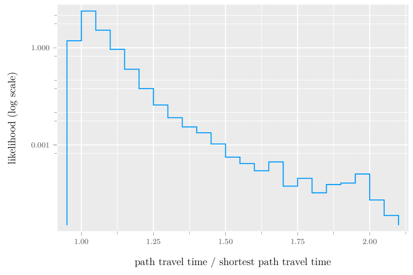
Figure 2: Comparison of path travel time and shortest path, the x axis shows the ratio while the y axis shows the likelihood. Note that the y axis is log scaled. The area under the curve is 1.

We end this section with a few remarks. Our experiments showed little sensitivity to the initialization. Effects of regularization depend on the data-set size, the more data the less regularization is required. As expected, low learning rates lead to more steps in the optimization loops. Some results are shown in Appendix D. As initialization, we propose the parameters $\boldsymbol{b}_{0}=-2$, $\boldsymbol{T}_{0}=\boldsymbol{T}_{\text{min}}/0.9$, $\log\eta=-2$ and $\lambda=0$. Another viable alternative is to initialize using the solution of the two-step method and use our method to improve the estimation.

5.3 Results – Synthetic data

In this section we analyze results on data that has been simulated on a grid network with a path choice model we posit (see Appendix C for details). Since we have access to observations at different levels of granularity, we can choose to use path observations, or only observed OD times (as in the Yellow Cab data). This results in diffrent versions of our method: with/without regularization (reg.), with/without path observations.

We start with a qualitative analysis based on results shown in Figure 3. It contains a visualization of $\boldsymbol{T}$ for the methods where ground truth is shown in (a). The RMSLE between the estimated $\hat{\boldsymbol{T}}$ and the ground truth is below 0.14 for our model, below 0.08 for our model with paths, and 0.22 for BDJM method. However, we can see that our estimate of $\boldsymbol{T}$ is more accurate while all methods have a similar RMSLE (ours is 0.31 while BDJM is 0.33). This highlights one of the weaknesses of measuring model performance with RMSLE. One alternative would be to compare predicted travel time for known paths but it is not always possible.

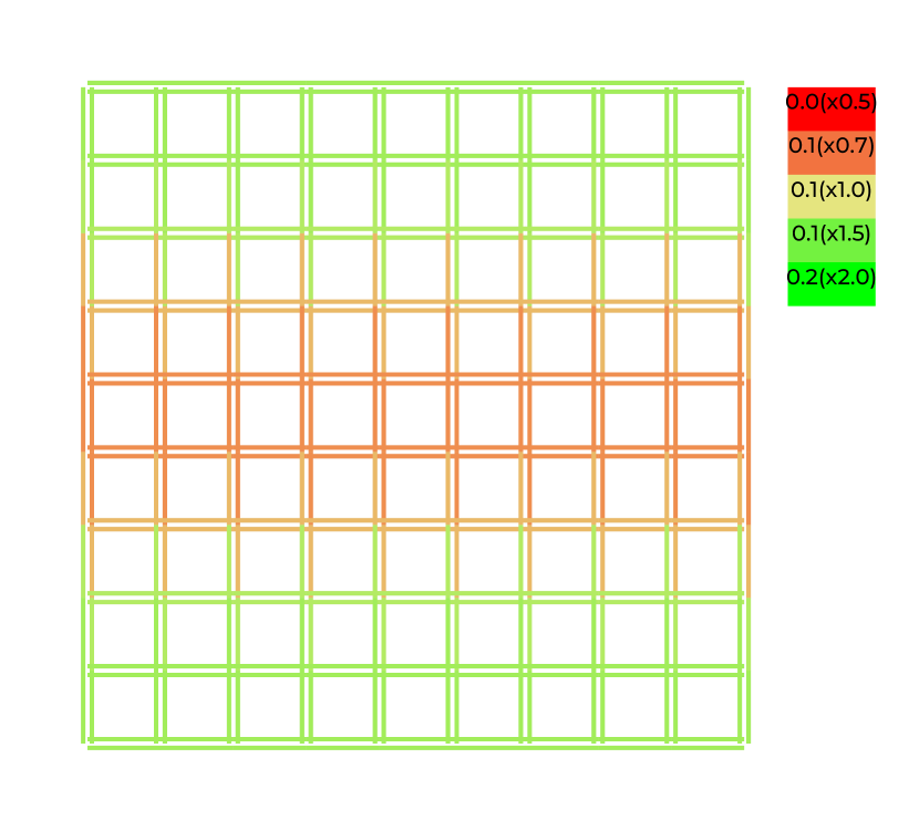
(a) Ground truth

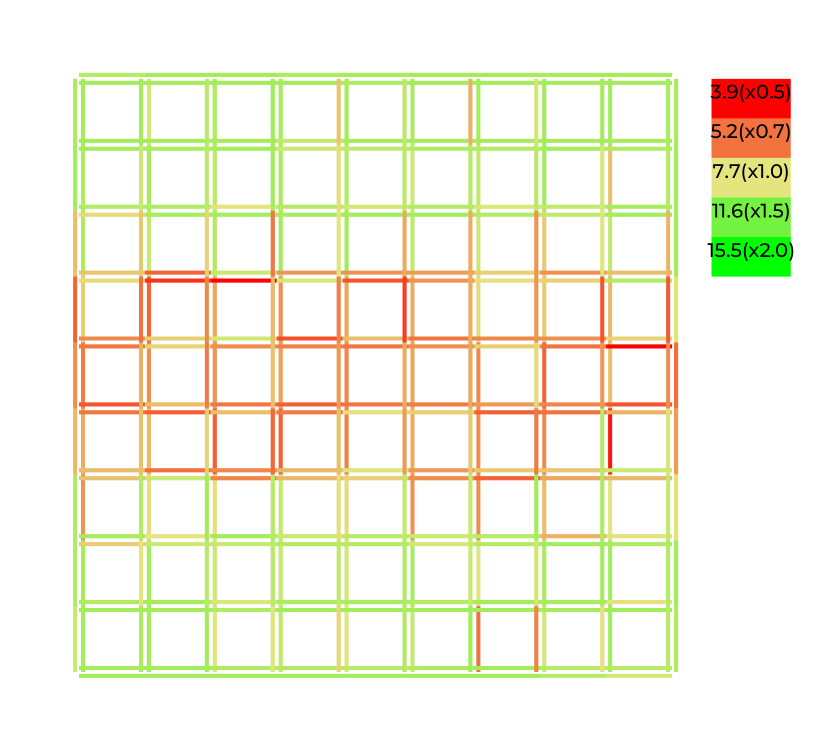
(b) Ours

(c) Ours reg.

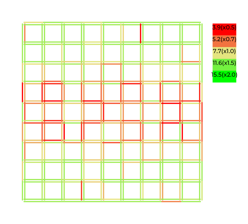
(d) BDJM’s method

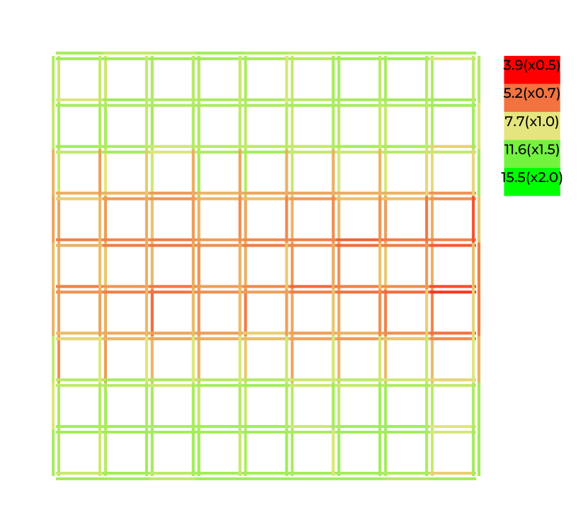
(e) Ours path

(f) Ours path and reg.

Figure 3: Comparison of estimated arc travel time matrix, same color scale for all figure. reg. stands for regularized.

Next we turn our attention to an analysis of the parameter estimates, comparing to the ground truth values. Here the main objective is to compare our method’s estimates to ground truth values, and those obtained using existing approaches, i.e., assuming travel time is exogenous and given. We assume that it is 90% of free-flow travel time, or the two-step approach that estimates travel time using the BDJM method.

The results are reported in Table 3. Note that we compare parameter ratios. The free flow and two-step approach (last two rows) cannot retrieve the ground truth parameter ratios. Given that recursive logit has been used to generate the data, the path choice assumption in the first step is misspecified. The bias in the travel times are absorbed by the travel time parameter estimate. On the contrary, our method achieves parameter estimate ratios close to the ground truth ratio. While $\boldsymbol{b}$ is well estimated in all cases, the methods with observed path have a much better estimate of $\boldsymbol{T}$.

Finally we not that, unsurprisingly, having path observations makes the problem deterministic and much easier to solve.

Model name log-likelihood $\hat{\boldsymbol{b}}_{\text{travel time}}/\boldsymbol{b}_{\text{left turn}}$ Ground truth $-1.65$ $1.00$ Ours $-1.83$ $1.01$ Ours with reg. $-1.70$ $1.07$ Ours with path $-1.67$ $0.96$ Ours with path and reg. $-1.66$ $1.01$ Free-flow (90%) $-2.14$ $0.78$ Two-step approach $-1.88$ $0.72$

Table 3: Comparison of the log-likelihood. $\boldsymbol{b}_{\text{u-turn}}$ is set to -5.

6 Conclusion

We proposed a mixture to model traffic that is compatible with a large class path choice models and loss functions. It is designed to estimate arc travel time and path choice model parameters simultaneously. We showed that by marginalizing the unobserved variables and using stochastic gradient estimates, we obtain a maximum likelihood estimation even for observations at different level of granularity. We showed that we can mix different data type when computing the MLE without needing to use a linear combination of losses as objective. We also showed that optimizing this mixture is fast. Furthermore, we showed that estimating recursive models like Fosgerau et al. (2013), and the method of Bertsimas et al. (2019) result in maximum likelihood estimates of this mixture. In the process we also showed that the common methodology for estimating path choice models could lead to biased results or bad results.

While our method has shown great potential, it needs to be tested on more path choice models, datasets, and $t$ distributions $\mathcal{N}$. As mentioned in Section 4, the only requirement is that the path choice model is differentiable. However, further experiments are needed to confirm that our methodology works in practice on this large class of path choice models. We chose Manhattan to make the experimental section similar to the one of Bertsimas et al. (2019). However, it is possible to see different results when the level of congestion and similarity to a grid changes. We do not have mixed data to show that using travel time data does improve the classical setting. Finally, estimating the variance of parameter estimates is of interest.

Appendix A Recursive logit estimation and gradients

Let $d$ be an absorbing state with no outgoing arcs and zero incoming utility i.e., $v(d|i)=0$ for all nodes $i$ connected to the absorbing state. Let $M^{d}$ be a $|N|$ by $|N|$ matrix where

$$M^{d}_{ij}=\begin{cases}\exp[v(j|i)]&\text{if $j\in N(i)$}\\ 0&\text{o.w.}\end{cases} (a,b)\in N^{2},$$ (45)

and $z^{d}$ be a vector with $|N|$ entries such that $z^{d}_{i}=\exp[w(i;d)]$. By taking the exponential of both sides of the log sum exp solution of the Bellman equation (7), Fosgerau et al. (2013) rewrite it as a system of linear equation

$$z^{d}=M^{d}z^{d}+b^{d},$$ (46)

where $b^{d}$ is a vector like $z^{d}$ where all entries are zero except the entry corresponding to the absorbing state is one. The probability is given by

$$\mathbb{P}(j|i;d)\propto M^{d}_{ij}z^{d}_{j}.$$ (47)

This formulation leads to $N$ difference system of equations with different left-hand sides. To reduce the number of factorizations needed to solve the $N$ systems, Mai et al. (2018) proposes to extend the original graph with one node that will be the absorbing state for all destination arcs. However, arcs are added for each destination separately. Let $M^{0}$ be a matrix-like $M^{d}$ with a size of $|N|+1$ by $|N|+1$; we define $U^{d}$ as the matrix containing the exponent of the utility of the arcs connected to the absorbing state (the entries are binary), the equation (46) is equal to

$$z^{d}=(M^{0}+U^{d})z^{d}+b^{d}.$$

Since the absorbing state is the last entry, $z^{d}_{|N|+1}$ is one. As such, $U^{d}z^{d}$ is just the last column of $U^{d}$ and independent of $z$. We define $t^{d}=U^{d}z^{d}$ and rewrite the system as

$$z^{d}=M^{0}z^{d}+(t^{d}+b^{d}).$$

Now the right-hand side $I-M^{0}$ is the same for all destinations; hence the factorization is also the same. Here on, we use $M$ to refer to $M^{0}$.

The log-likelihood of path $r$ from $o$ to $d$ can be written as

$$\ln\mathbb{P}(r)=-w(o;d)+\sum_{(i,j)\in r}v(j|i).$$ (48)

The derivative of $v(j,i)$ is trivial. The derivative of $w(o;d)$ is written using $Z_{od}$ since $w(o;d)=\ln Z_{od}$. Mai et al. (2018) showed that

$$\frac{\partial Z}{\partial x}=(I-M)^{-1}\frac{\partial M}{\partial x}Z.$$ (49)

It is worth mentioning that ${\partial M}/{\partial\boldsymbol{T}_{ij}}$ has only one non-zero element. As such, it does not need to do the full matrix multiplication i.e.,

$$\frac{\partial Z}{\partial\boldsymbol{T}_{ij}}=\frac{\partial M_{ij}}{\partial\boldsymbol{T}_{ij}}(I-M)^{-1}_{i:}Z_{:j}.$$

It is possible that $Z_{od}$ becomes too small during training which can cause $1/Z_{od}$ to become too big. To deal with this, we clamp $Z_{od}$ between 1e-250 and infinity before inverting. It is also possible that Z becomes negative. In those cases, we take the absolute value.

Appendix B Implementation details

There implementation details are:

Using sparse matrices to represent the data.

We use column major arrays and Compressed Sparse Columns (CSC) arrays to represent the data. The transition matrix must be represented in a way that allows sampling transitions by only reading the non-zero entries in a cache-friendly way i.e., with CSC matrices, the transition vectors are the columns not the rows. We note that operations we used on sparse matrices on a single CPU core are faster than dense matrices on GPU. The difference becomes more and more exaggerated as the size of the graph increases. Another difference is the cost of RAM and the number of parallel operations we can do in multi-core systems.

Reusing sparsity pattern.

Since many of our matrices have the same sparsity pattern (if we remove the absorbing state of the matrix), we reuse the structure vectors to reduce memory usage significantly. Furthermore, we do many operations directly on the non-zero vectors.

Multi-threading.

A significant improvement comes from using multi-threading. Our method can usually be split by destination or OD pairs (depending on the path choice model) and scales almost linearly with the number of threads.

Calculating the gradient analytically.

The analytical gradient can have better numerical precision and performance than automatic differentiation (AD). Furthermore, AD engines cannot optimize the calculations enough. When we calculate gradient manually, we avoid re-computation and computing values we do not need. For instance, in (49) we only calculate the rows that we need from $(I-M)^{-1}$. We achieve this by solving the system with the transpose of the LU factorization on the useful columns of $(I-M)^{-\top}$.

Appendix C Data processing

For the real data, just like Bertsimas et al. (2019), we first download a recent map of the city from Open Street Map (OSM) (OpenStreetMap contributors, 2022) and cut out the parts outside a polygon that encircles the target (Manhattan). We fill the missing speed limit using official maximum speed limits based on the type of road. We remove all none intersection nodes as long as adding arcs to bypass that node will not create arcs larger than 100 meters. A non-intersection node is a node that has two neighbors such that they are all part of a one-way or two-way path. We keep stop signs, and red light nodes unless the crossing is at most 50 meters or 100 nodes away from a red light or stop sign. We split arcs longer than 200 meters into two arcs connected to a new node in the middle of the two nodes. Note that we keep dead ends. We repeat this process until we cannot remove any more nodes. We then take the largest connected component of the graph. This transformation keeps the topology intact as we can easily interpolate the original graph’s travel time. This process removes many nodes whose sole purpose is to convey the geometry of the streets, as OSM does not support curved arcs.

We match the origin and destination from the cab dataset using the nearest node with an upper bound of 100 meters on the distance between the observation and the node. We remove trips that are shorter than 30 seconds or longer than 3 hours or have an average speed of less than 1 meter per second or greater than the city’s maximum speed on the highway (50 miles per hour in the case of NYC) on the shortest path connecting the origin and destination. We then take the data observed in a time range of day group (workdays, weekends, etc.). We show the results in Figure 4.

We take a training and validation set with 100, 1,000, 10,000, 100,000, and 200,000 observations. The test set contains 100,000 observations. We use the data from April 2016 to validate the code and show the results on May 2016.

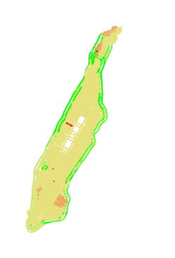
Figure 4: Map of Manhattan at free-flow speed.

For the synthetic tests, we simulated data on a 10 by 10 grid where each node is 600 meters away from its neighbors. The minimum and maximum speeds are 5.5 and 10 m/s, respectively. The travel time of the arc that ends in the $i$th column and $j$th row is $600/10-3(j-3300)^{2}/3300^{2}$ clamped between the legal speed. We use $\boldsymbol{b}=(-2,-2,-5)^{\top}$ to generate 10,000 samples for the train, test, and validation sets. We generate 5 trajectories between each (o, d) uniformly. We multiply each observed travel time by a sample from the log-normal $(0.1,\sqrt{0.1})$. We show the grid in Figure 3(a).

Appendix D Hyper parameter and intialization figures

In this section we analyze the effect of hyper parameters on our model. We take the best hyper parameter found on the Manhattan late morning dataset with 10,000 observations and change one of the hyper parameters in each figures and train the model. We show both the training curve for different parameters and the final validation loss.

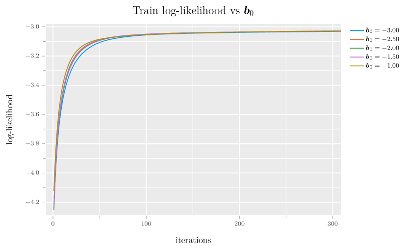
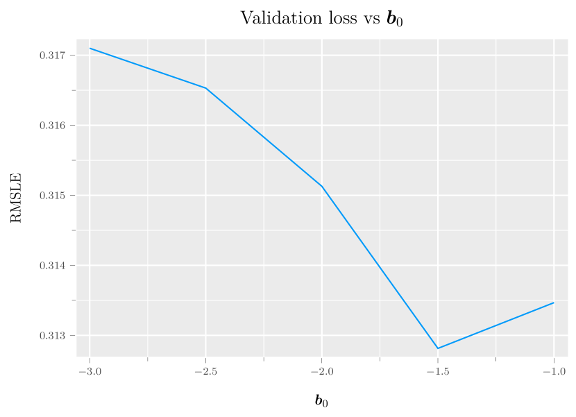
Figure 5: Sensitivity of our method to the choice of $\boldsymbol{b}_{0}$.

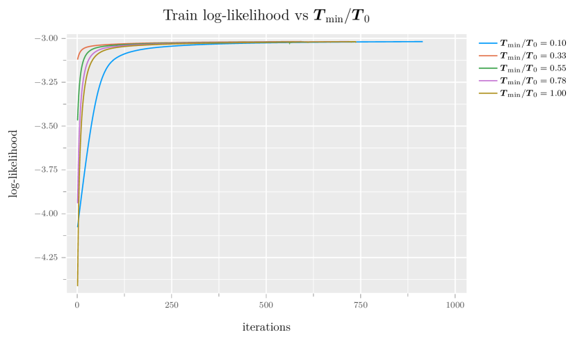
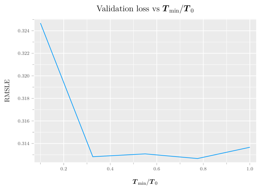
Figure 6: Sensitivity of our method to the choice of $\boldsymbol{T}_{0}$.

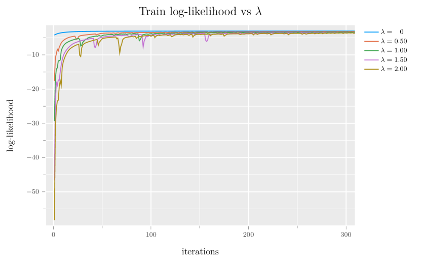
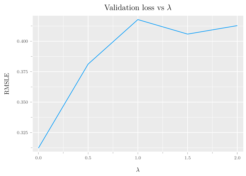
Figure 7: Sensitivity of our method to the choice of $\lambda$.

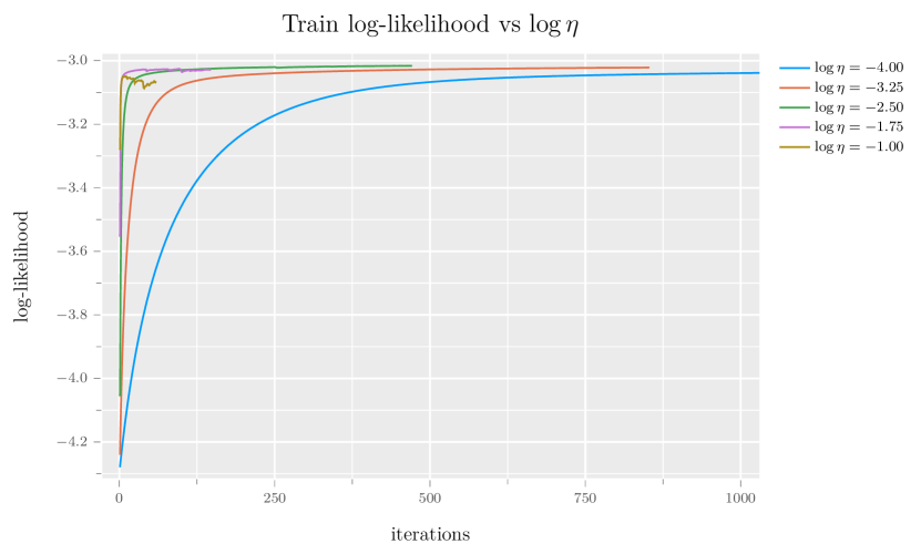
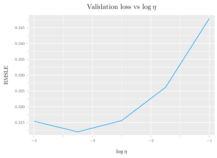
Figure 8: Sensitivity of our method to the choice of $\eta$. Logarithmic scale in the learning rate.

References

- Abdzaid Atiyah et al. (2020) Abdzaid Atiyah, I., Mohammadpour, A., Ahmadzadehgoli, N., and Taheri, S. Fuzzy C-means clustering using asymmetric loss function. Journal of Statistical Theory and Applications, 19(1):91–101, 2020.
- Audet et al. (2021) Audet, C., Digabel, S. L., Montplaisir, V. R., and Tribes, C. Nomad version 4: Nonlinear optimization with the MADS algorithm. arXiv preprint arXiv:2104.11627, 2021.
- Baillon and Cominetti (2008) Baillon, J.-B. and Cominetti, R. Markovian traffic equilibrium. Mathematical Programming Series B, 111:33–56, 2008.
- Bellman (1954) Bellman, R. The theory of dynamic programming. Bulletin of the American Mathematical Society, 60(6):503–515, 1954.
- Bertsimas et al. (2019) Bertsimas, D., Delarue, A., Jaillet, P., and Martin, S. Travel time estimation in the age of big data. Operations Research, 67(2):498–515, 2019.
- Bezanson et al. (2017) Bezanson, J., Edelman, A., Karpinski, S., and Shah, V. B. Julia: A fresh approach to numerical computing. SIAM review, 59(1):65–98, 2017.
- Chen et al. (2014) Chen, B. Y., Yuan, H., Li, Q., Lam, W. H., Shaw, S.-L., and Yan, K. Map-matching algorithm for large-scale low-frequency floating car data. International Journal of Geographical Information Science, 28(1):22–38, 2014.
- DasGupta (2008) DasGupta, A. Asymptotic theory of statistics and probability, volume 180. Springer, 2008.
- de Moraes Ramos et al. (2020) de Moraes Ramos, G., Mai, T., Daamen, W., Frejinger, E., and Hoogendoorn, S. Route choice behaviour and travel information in a congested network: Static and dynamic recursive models. Transportation Research Part C: Emerging Technologies, 114:681–693, 2020.
- Dial (1971) Dial, R. B. A probabilistic multipath traffic assignment model which obviates path enumeration. Transportation Research, 5(2):83–111, 1971.
- Ding-Mastera et al. (2019) Ding-Mastera, J., Gao, S., Jenelius, E., Rahmani, M., and Ben-Akiva, M. A latent-class adaptive routing choice model in stochastic time-dependent networks. Transportation Research Part B: Methodological, 124:1–17, 2019.
- Fisk (1980) Fisk, C. Some developments in equilibrium traffic assignment. Transportation Research Part B: Methodological, 14(3):243–255, 1980.
- Fosgerau et al. (2013) Fosgerau, M., Frejinger, E., and Karlstrom, A. A link based network route choice model with unrestricted choice set. Transportation Research Part B-Methodological, 56:70–80, 2013.
- Fosgerau and Karlström (2010) Fosgerau, M. and Karlström, A. The value of reliability. Transportation Research Part B: Methodological, 44(1):38–49, 2010.
- Freedman (2006) Freedman, D. A. On the so-called “huber sandwich estimator” and “robust standard errors”. The American Statistician, 60(4):299–302, 2006.
- Frejinger and Zimmermann (2021) Frejinger, E. and Zimmermann, M. Route choice and network modeling. In International Encyclopedia of Transportation, volume 4, pages 496–503. Elsevier, 2021.
- Gao et al. (2010) Gao, S., Frejinger, E., and Ben-Akiva, M. Adaptive route choices in risky traffic networks: A prospect theory approach. Transportation Research Part C: Emerging Technologies, 18(5):727–740, 2010.
- Kingma and Ba (2014) Kingma, D. and Ba, J. Adam: A method for stochastic optimization. arXiv preprint arXiv:1412.6980, 2014.
- LeCun et al. (2007) LeCun, Y., Chopra, S., Hadsell, R., Ranzato, M., and Huang, F. j. Energy-Based Models. The MIT Press, 2007.
- Mai et al. (2018) Mai, T., Bastin, F., and Frejinger, E. A decomposition method for estimating recursive logit based route choice models. Euro Journal on Transportation and Logistics, 7(3):253–275, 2018.
- Mai et al. (2021) Mai, T., Yu, X., Gao, S., and Frejinger, E. Routing policy choice prediction in a stochastic network: Recursive model and solution algorithm. Transportation Research Part B: Methodological, 151:42–58, 2021.
- McFadden (1977) McFadden, D. Modelling the choice of residential location. Transportation Research Record, 1977.
- Mohamed et al. (2020) Mohamed, S., Rosca, M., Figurnov, M., and Mnih, A. Monte Carlo Gradient Estimation in Machine Learning. Journal of Machine Learning Research, 21(132):1–62, 2020.
- Mori et al. (2015) Mori, U., Mendiburu, A., Álvarez, M., and Lozano, J. A. A review of travel time estimation and forecasting for advanced traveller information systems. Transportmetrica A: Transport Science, 11(2):119–157, 2015.
- MOSEK ApS (2022) MOSEK ApS. MOSEK optimization suite. Version 9.3., 2022.
- New York City Taxi and Limousine Commission (2016) New York City Taxi and Limousine Commission. New york city taxi trip data, 2016. Data downloaded in June 2022 from https://registry.opendata.aws/nyc-tlc-trip-records-pds.
- Nikolova and Stier-Moses (2014) Nikolova, E. and Stier-Moses, N. E. A mean-risk model for the traffic assignment problem with stochastic travel times. Operations Research, 62(2):366–382, 2014.
- Oh et al. (2015) Oh, S., Byon, Y.-J., Jang, K., and Yeo, H. Short-term travel-time prediction on highway: A review of the data-driven approach. Transport Reviews, 35(1):4–32, 2015.
- OpenStreetMap contributors (2022) OpenStreetMap contributors. OpenStreetMap project database, 2022. Downloaded in June 2022 from https://overpass-api.de.
- Prato (2009) Prato, C. G. Route choice modeling: past, present and future research directions. Journal of Choice Modelling, 2(1):65–100, 2009.
- Quddus and Washington (2015) Quddus, M. and Washington, S. Shortest path and vehicle trajectory aided map-matching for low frequency gps data. Transportation Research Part C: Emerging Technologies, 55:328–339, 2015.
- Rust (1987) Rust, J. Optimal replacement of GMC bus engines: An empirical model of Harold Zurcher. Econometrica, 55(5):999–1033, 1987.
- Rust (1988) Rust, J. Maximum likelihood estimation of discrete control processes. SIAM Journal on Control and Optimization, 26(5):1006–1024, 1988.
- Williams (1992) Williams, R. Simple statistical gradient-following algorithms for connectionist reinforcement learning. Machine Learning, 8(3-4):229–256, 1992.
- Zhu et al. (1997) Zhu, C., Byrd, R., Lu, P., and Nocedal, J. Algorithm 778: L-BFGS-B: Fortran Subroutines for Large-Scale Bound-Constrained Optimization. ACM Transactions on Mathematical Software, 23(4):550–560, 1997.
- Ziebart et al. (2008) Ziebart, B. D., Maas, A., Bagnell, J. A., and Dey, A. K. Maximum entropy inverse reinforcement learning. In Proceedings of the Twenty-Third AAAI Conference on Artificial Intelligence, volume 8, pages 1433–1438, 2008.
- Zimmermann and Frejinger (2020) Zimmermann, M. and Frejinger, E. A tutorial on recursive models for analyzing and predicting path choice behavior. EURO Journal on Transportation and Logistics, 9(2):100004, 2020.