Staircase formation in unstably stratified double diffusive finger convection

Abstract

Double diffusive staircases are investigated experimentally in a fluid layer with a stabilizing temperature gradient and a destabilizing gradient of ion concentration. Gradients of temperature and ion concentration are maintained in a steady state within an electrochemical system. Staircases are observed even if the density stratification is unstable. None of the previously proposed mechanisms for staircase formation can be recognized in the experiments. Ion transport through fingers which are part of a staircase is not the same as transport through fingers extending through the entire cell. Fingers cease to exist if the diffusive heat transport between neighboring fingers is insufficient.

I Introduction

Double diffusive convection Radko (2013) is a form of convection in which the density of the convecting fluid is determined by two different quantities which diffuse at different rates. The study of double diffusive convection has a long history in oceanography because the density of ocean water depends on both temperature and salinity whose diffusivities differ by two orders of magnitude. Double diffusive convection can give rise to spectacular patterns, such as salt finger convection in a water layer with stable density stratification, or convection flows split into vertically stacked layers. These effects motivated numerous laboratory experiments. Most of these study transient phenomena by setting up initial temperature and salinity gradients which are then consumed by convection. Steady states are more difficult to realize. They can be produced either with a system of membranes and tanks Krishnamurti (2003, 2009) or with an electrodeposition cell Hage and Tilgner (2010); Kellner and Tilgner (2014). The second method is employed in the experiments presented in this paper.

The electrodeposition cell is filled with a solution of $CuSO_{4}$ in $H_{2}SO_{4}$. Two copper electrodes placed at the top and bottom of the cell are regulated in temperature which maintains a temperature gradient within the cell. If a voltage difference is applied between the upper and lower plates, an electric current flows through the electrodes and the electrolyte which is carried by copper ions detached from one electrode and deposited on the other. The copper ion concentration in the electrolyte plays the role of salinity. However, for copper ions in an electrolyte to behave like salt in ocean water, the ions should diffuse and be advected by the flow, but they should not drift in an electric field due the potential difference between the electrodes. This is the reason for filling the cell with acid. The highly mobile protons in the acid create microscopic charged layers next to the electrodes without participating in the electrochemistry and screen the interior of the cell from any electric field.

This electrochemical system was originally used to study Rayleigh-Bénard convection Goldstein, Chiang, and See (1990) and later double diffusive finger convection Hage and Tilgner (2010) and the transition from large scale convection rolls to fingers Kellner and Tilgner (2014). The focus of the new experiments is on double diffusive staircases. These are stacks of layers filled alternatingly with finger convection or motion organized into large scale convection rolls. Staircases have been observed both in the oceans and in laboratory experiments. However, the mechanism by which they form and hence the conditions necessary for their existence remains controversial. It is therefore of interest to search for staircases in the electrochemical system.

Layering and staircases in double diffusive systems are studied in various contexts, for example in chemical engineering and solidification processes Kumar, Srivastava, and Karagadde (2018). Oceanography is the richest field of application, which includes the study of the properties of staircases once they have formed, as for example the interaction of internal gravity waves with staircases Radko (2020), and more fundamentally the study of the mechanisms by which staircases form. There are two distinct cases to be investigated. In the ”diffusive” case, the salt gradient stabilizes the fluid whereas the temperature gradient destabilizes it and drives the motion Radko (2016); Brown and Radko (2019); Yang et al. (2022); Ma and Peltier (2022). The present paper is solely concerned with the opposite configuration, or the ”finger” case, with a stabilizing temperature and a destabilizing salinity gradient. The most successful theories of staircase formation in this second case are based on a parametrization of heat and salinity fluxes in terms of local gradients of temperature and salinity Radko (2003); Sellmach et al. (2011); Traxler et al. (2011). This approach was extended to non uniform gradients Ma and Peltier (2021) and received additional numerical support recently Yang et al. (2020). However, these theories suffer from an ultraviolet catastrophe in the sense that they yield unbounded growth rates at high wavenumbers. There is therefore an ongoing effort to improve these theories Radko (2014, 2019) and staircase formation remains an open field of research.

Section II reviews the control parameters relevant to the electrodeposition cell briefly described above and in more detail in ref. Hage and Tilgner, 2010. Section III qualitatively describes the observed flows while section IV discusses various mechanisms which might possibly induce the transitions between the different types of flows. Section V finally deals with the ion transport in the convection flows.

II The Experiment

The material properties characterizing the fluid in the electrodeposition cell are the kinematic viscosity of the fluid $\nu$, the diffusivities of temperature and ion concentration, $\kappa$ and $D$, and two expansion coefficients $\alpha$ and $\beta$ determining variations of density $\rho$ as a function of temperature $T$ and copper ion concentration $c$ around a reference state with density, temperature, concentration and pressure $\rho_{0}$, $T_{0}$, $c_{0}$ and $p_{0}$ via

$$\alpha=-\frac{1}{\rho_{0}}\left(\frac{\partial\rho}{\partial T}\right)_{c_{0},T_{0},p_{0}}~{}~{}~{},~{}~{}~{}\beta=\frac{1}{\rho_{0}}\left(\frac{\partial\rho}{\partial c}\right)_{c_{0},T_{0},p_{0}}.$$ (1)

Both $\alpha$ and $\beta$ are positive. The remaining parameters are the gravitational acceleration $g$, the cell height $L$, and the temperature and concentration differences applied across the cell, $\Delta T$ and $\Delta c$, defined as

$$\Delta T=T_{\rm{bottom}}-T_{\rm{top}}~{}~{}~{},~{}~{}~{}\Delta c=c_{\rm{top}}-c_{\rm{bottom}}$$ (2)

with the subscripts indicating the boundary at which temperature $T$ or concentration $c$ are evaluated. The concentration difference $\Delta c$ is known because the cell is always operated at the limiting current Hage and Tilgner (2010); Goldstein, Chiang, and See (1990). In that case, $\Delta c=2c_{0}$, where $c_{0}$ is the average concentration of copper in the solution.

Adimensional parameters are more convenient for the comparison with other double diffusive systems. Four non-dimensional numbers are necessary to specify all control parameters. A possible choice for these four parameters are the Prandtl and Schmidt numbers, $Pr$ and $Sc$, defined as

$$Pr=\frac{\nu}{\kappa}~{}~{}~{},~{}~{}~{}Sc=\frac{\nu}{D}.$$ (3)

together with the thermal and chemical Rayleigh numbers, $Ra_{T}$ and $Ra_{c}$, given by

$$Ra_{T}=\frac{g\alpha\Delta TL^{3}}{\kappa\nu}~{}~{}~{},~{}~{}~{}Ra_{c}=\frac{g\beta\Delta cL^{3}}{D\nu}.$$ (4)

The material constants $Pr$ and $Sc$ are nearly constant for the measurements reported here with $Pr\approx 9$ and $Sc\approx 2000$.

With the sign conventions for $\Delta T$ and $\Delta c$, a stabilizing temperature and a destabilizing concentration gradient are characterized by a negative $Ra_{T}$ and a positive $Ra_{c}$. This combination of signs was realized in all experiments described in this paper.

The density ratio $\Lambda$ is not independent of the four control parameters just introduced but is a combination of them which quantifies the ratio of thermal over chemical buoyancy and which will prove convenient below:

$$\Lambda=\frac{Ra_{T}}{Ra_{c}}\frac{Sc}{Pr}=\frac{\alpha\Delta T}{\beta\Delta c}.$$ (5)

The observables extracted from the measurements will also be reported in terms of adimensional numbers. First of all, there is the Sherwood number, which is directly proportional to the number of ions transported from top to bottom divided by the purely diffusive current, which means that the Sherwood number is given by

$$Sh=\frac{j\,L}{z\,F\,D\,\Delta c}$$ (6)

if $j$ is the current density, $z$ the valence of the ion ($z=2$ for $Cu^{2+}$), and $F$ is Faraday’s constant. The Sherwood number is therefore the adimensional analog of the electric current through the cell which is convenient to measure.

The velocity field was characterized by particle image velocimetry (PIV). A vertical plane near the middle of the cell was illuminated with a thin laser sheet and observed at right angles with a camera. In a Cartesian coordinate system in which $z$ points upwards and the $x$- axis lies horizontally within the plane of illumination, the PIV measurements yield the velocity components $v_{x}$ and $v_{z}$ as a function of space and time. Let us denote a time average by an overline. The Reynolds number $Re$ extracted from these measurements is defined as

$$Re=\frac{L}{\nu}\left(\frac{1}{A}\int(\overline{v_{x}^{2}}+\overline{v_{z}^{2}})dA\right)^{1/2}$$ (7)

where the integral extends over the entire illuminated plane of surface $A$. It will be useful for the detection of staircases to define rms amplitudes of the fluctuations of $v_{x}$ and $v_{z}$ as a function of height $z$ as

$$\langle v_{x}^{2}\rangle(z)=\frac{1}{b}\int_{0}^{b}\overline{v_{x}^{2}}dx-\left(\frac{1}{b}\int_{0}^{b}\overline{v_{x}}dx\right)^{2}$$ (8)

and

$$\langle v_{z}^{2}\rangle(z)=\frac{1}{b}\int_{0}^{b}\overline{v_{z}^{2}}dx-\left(\frac{1}{b}\int_{0}^{b}\overline{v_{z}}dx\right)^{2}$$ (9)

where the integrals extend over the width $b$ of the plane of illumination.

Finally, the PIV measurements also allow the measurement of the finger thickness $d$ which is expressed in adimensional form as the ratio $d/L$. The finger thickness is determined by counting the number of changes of sign in the vertical velocity $v_{z}$ at any given height $z$ which yields an instantaneous profile $d(z)$. The time average of this profile is nearly constant over extended intervals of height within the layers identified below which allows us to define a finger thickness $d$ for every layer.

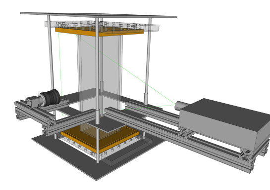
Figure 1: (Color online) Schematic view of the apparatus. Top and bottom copper electrodes are bordered by plexiglass plates for thermal insulation and to mechanically hold the cell together. Laser and camera can be moved vertically to observe the flow in the cell at different heights.

A schematic view of the apparatus is shown in fig. 1. Copper plates at the top and bottom of the cell served as electrodes. A voltage was applied to the cell with the right polarity to detach copper ions at the top electrode and to reattach them at the bottom. Thermally regulated water flowing through channels milled into the copper plates held the temperature of the electrodes nearly constant and maintained temperature differences of 1.5-50 $K$ between top and bottom plates. The temperature of the plates was monitored with thermistors introduced in narrow holes drilled into the copper. Plate temperature was stable to within $0.1K$. The cell was filled with $CuSO_{4}$ and 1 molar $H_{2}SO_{4}$.

Ohmic heating in the electrolyte has negligible effect on buoyancy because there is no electric dissipation in the bulk of the cell which is screened from the electric field by the protons of the acid. All dissipation occurs next to the temperature regulated plates in thin layers whose thickness $l$ is on the order of a Debye length Probstein (1995). This length is a few nanometers in the experiments. Temperature variation due to ohmic dissipation is small because heat diffuses rapidly over such a short length scale. For a quantitative estimate of the temperature perturbation, we may model the electric dissipation as heat sources of amplitude $Q$ distributed uniformly within two layers of thickness $l$. If $j$ is the electric current density and $U$ the total voltage drop across the cell, $Q$ must be chosen as $Q=jU/(2l)$ with a factor 2 because there are two layers, one next to each electrode. To estimate the effect of these heat sources, we solve the heat diffusion equation $k_{T}\frac{\partial^{2}}{\partial z^{2}}T+Q=0$ with the boundary conditions that $T=0$ at $z=0$ and $z=l$ and with $k_{T}$ being the heat conductivity. This equation is solved by $T(z)=Qd^{2}/(2k_{T})\cdot z(l-z)/d^{2}$. The maximal temperature deviation reached within the layer is therefore $Qd^{2}/(2k_{T})$. It follows that for typical parameters of the experiment with $jU<50W/m^{2}$, $k_{T}\approx 0.5W/(Km)$ and $l\approx 10nm$, the electrolyte is heated by less than $1\mu K$ due to ohmic dissipation and that electric dissipation causes no significant buoyancy in the experiments.

The main difference with the previous experiments on the same system Hage and Tilgner (2010); Kellner and Tilgner (2014) is the size of the cell. The new experiments used cells with heights $40cm$ and $80cm$ to reach high Rayleigh numbers. All cells had a square cross section of $10cm\times 10cm$. The field of view of the camera during PIV measurements could not cover the entire height of the cell. Camera and laser were therefore mounted on rails so that they could be moved vertically. Pictures were recorded for several seconds at any given height level before camera and laser were moved up or down to record a different section of the cell. This motion was repeated in cycles to avoid any bias that might be introduced by measuring velocity in one part of the cell at an early time and in another part of the cell at a late time. Nonetheless, the velocity measurements were not obtained simultaneously at all heights so that velocity profiles show discontinuities at the heights separating two sections pictured by the camera during the measurements. These discontinuities provide us with a measure of the uncertainty in the velocity measurements due to insufficient time averaging.

Another feature introduced by taller cells are longer transients because the turn over time of convection is increased. In addition, it takes longer to form and equilibrate a staircase than to establish salt fingers spanning the entire cell, which was the dominant flow structure in the earlier experiments. The approach to the states containing staircases will be exemplified in fig. 7. The natural time scale for the transient is the time it takes fluid within fingers to cross the cell. This transit time was between 15 minutes and 2 hours. Control parameters were typically held constant for one day which corresponds to 12 to 96 transit times. Long transit times arise if $|Ra_{T}|$ is large, which generally results in a single finger layer that reaches equilibrium after few transit times. The staircases, whose final states are attained after a more complicated history, occur at smaller $|Ra_{T}|$ at which all velocities tend to be larger so that more transit times fit into one day.

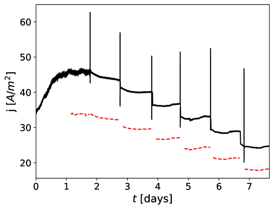
Figure 2: (Color online) Current density $j$ as a function of time for a series of measurements at $Ra_{c}=1.12\times 10^{13}$. The current density is computed as the total current through the cell divided by the cross section of the cell. The continuous line shows the measured current density, while the dashed line shows the value of the current density corrected for the roughening of the electrodes.

Long transients and data accumulation periods are a problem in the electrochemical system because the plates age. The extraction and deposition of copper roughens the electrodes and increases their surface areas which leads to an increased electric current through the cell. The ageing progresses more rapidly for more concentrated electrolytes and larger electric currents. However, the roughness of the electrodes saturates at a certain level. The ratio of the currents through cells equiped with old and new electrodes never exceeds 1.4.

The effect of ageing was largely avoided in the earlier experiments by frequently disassembling the cell to polish the electrodes. This procedure was not practical during the new set of experiments and the electrodes were left to age for longer before they were refurbished. One could choose at this stage to declare the cell with roughened electrodes to be the reference system and to be the main object of study. The precise state of the boundaries should not matter much if we are interested in a robust effect like staircase formation which also occurs in the oceans where the boundary conditions are yet different. But we also want to compare the new results with the older data obtained with well defined smooth boundaries so that an effort was made to correct electric current measurements for ageing effects.

A typical series of measurements started by filling the cell equipped with pristine electrodes with a solution with a certain concentration of cupric sulfate which fixed the $Ra_{c}$ for this series. The cell was filled from two temperature controlled buckets so that the temperature gradient within the cell immediately had the desired value for the first measurement. $Ra_{T}$ was subsequently varied from one value to another by modifying the temperature of the copper electrodes while the voltage was permanently applied. An example of a time series of the current through the cell from the moment the voltage is first applied to the next disassembly of the cell is shown in fig. 2. Short spikes occur in the current when PIV particles are injected. Each time the temperatures of the boundaries are modified, there is a rapid variation of the current which corresponds to a readjustment of the flow in response to the modified control parameters, which may then be followed by a slow variation of the current mostly due to the roughening of the electrodes. In order to correct for most of the ageing effect, intervals of time are marked manually in which the increase of the current is assumed to be entirely due to the surface modifications of the boundaries. During any of these intervals, the current changes by a certain factor. The current measured at all later times is divided by this factor. This yields a corrected current which is used in the computation of the Sherwood number. In the example of fig. 2, the current rises already by a factor of 1.3 between the early times and the first plateau reached approximately after one day. The flow was a single convection roll during that period with a transit time of less than 300 seconds. It was therefore assumed that the variation of current density after $t\approx 1hr$ was due to modifications of the electrode and that all surface roughening occurred during the first day, so that all currents measured thereafter were divided by this factor before they were introduced into the definition of the Sherwood number.

III Flow morphologies

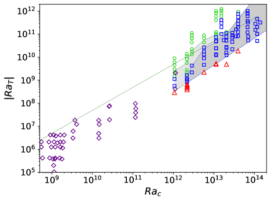
Figure 3: (Color online) Overview of the experiments in the $Ra_{c},Ra_{T}$-plane. Diamonds are data taken from ref. Hage and Tilgner, 2010. Circles represent states with fingers crossing the entire cell from top to bottom which is also the flow morphology for the diamonds. Squares are staircases defined as flow states in which the vertical profile of the horizontal rms velocity has a local maximum. Triangles represent flow states consisting of a convection roll without any fingers. The dark grey shaded area again indicates the region of existence of staircases, if a staircase is defined as a flow in which one of the convecting layers consists of up and down flows with a width comparable with half the cell width. The lightly shaded area contains all the parameter combinations for which the Sherwood number depends weakly on $|Ra_{T}|$ (as discussed in connection with fig. 8). The straight line indicates $|\Lambda|=1$.

Fig. 3 presents an overview of the combinations of $Ra_{T}$ and $Ra_{c}$ sampled during this and a previous study Hage and Tilgner (2010). The simplest types of flows found in the explored part of the parameter space are double diffusive fingers crossing the entire cell from top to bottom and convection rolls reminiscent of Rayleigh-Bénard convection. Fingers exist both at $|\Lambda|>1$ and $|\Lambda|<1$ even though the density stratification is unstable in the latter case. There is a well defined transition in going from fingers to convection rolls Kellner and Tilgner (2014) discussed further in section IV.

Numerous laboratory and field observations suggest that it should also be possible to generate double diffusive staircases in the electrodeposition cell. Staircases indeed appear, but only if $Ra_{c}>2\times 10^{12}$. A similar threshold of $Ra_{c}\approx 10^{11}$ has been found in numerical simulations Yang et al. (2020) in 3D periodic boxes with $Sc=21$ and $Pr=7$. The staircases in the experiment consist of a convection roll sandwiched between two finger layers each in contact with one of the boundaries. Staircases with more layers never developed. There are a few examples at the low $|Ra_{T}|$ end of the region of existence of staircases in fig. 3 in which the staircase forms only two layers, a convection roll above or below a finger layer.

As opposed to the very clear cut transition between flows consisting of a single convection roll and a single layer of fingers, the transition between the single finger layer and the staircase is more blurred and passes through intermediate stages. If $|Ra_{T}|$ is varied from large to small values at fixed $Ra_{c}$ with $Ra_{c}>2\times 10^{12}$ in fig. 3 (as shown in fig. 4 for $Ra_{c}=1.12\times 10^{13}$), one first finds straight fingers crossing the whole cell, but at lower $|Ra_{T}|$, the fingers thicken in the central region of the cell. At yet lower $|Ra_{T}|$, one visually identifies a central finger layer with thicker fingers than in the adjacent layers above and below. Finally, at even smaller $|Ra_{T}|$, the central layer is filled by a convection roll. The ratio of height over width of the central region is always around 1 or larger, so that an obvious definition of a convection roll in this context is a flow consisting of up and downwellings of roughly half the cell width. There is however some arbitrariness in what one wishes to call a staircase. A plausible criterion for the edge of a finger layer is the existence of a local maximum in the rms of horizontal velocity, because the vertical flow within the fingers needs to connect through horizontal motions at the ends of the fingers. However, as the example in fig. 5 shows, the maximum in the rms of horizontal velocity lies well within the convection roll and marks the edge of the velocity boundary layer inside the convection roll rather than the edge of the finger layer. A better indicator for the size of a finger layer therefore is a kink or sudden change in first derivative of the vertical profile of the rms of horizontal velocity, paired with plain visual inspection of PIV images. The height of finger layers $L_{f}$ determined in this fashion will be used below.

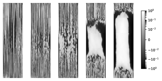
Figure 4: Grey scale maps of the vertical velocity normalized by the maximal absolute value of vertical velocity for $Ra_{c}=1.12\times 10^{13}$ and, from left to right, $|Ra_{T}|=1.22\times 10^{11}$, $1.01\times 10^{11}$, $4.97\times 10^{10}$, $2.44\times 10^{10}$ and $1.23\times 10^{10}$. Each panel is a time average over two hours.

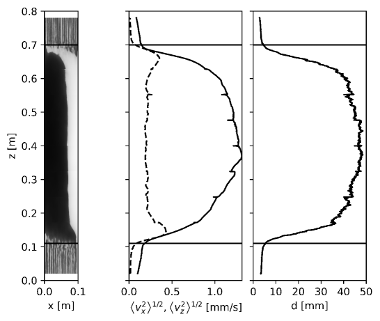
Figure 5: Map of the vertical velocity (left panel), variations of rms of horizontal and vertical velocity with height (central panel, dashed and continuous lines, respectively), and finger thickness as a function of height (right panel) for $Ra_{c}=6.89\times 10^{13}$ and $|Ra_{T}|=3.24\times 10^{11}$. All panels show results obtained from averaging over 46 hours. The horizontal lines show the heights that were identified as limits of the upper and lower finger layers according to the criterion described in the text.

As finger layers in staircases may border a convection roll or a less clearly classified internal layer, fig. 3 shows the region of existence of staircases according to two different definitions: staircases whose central region consist of a broad up and down flow reminiscent of Rayleigh-Bénard convection, and staircases in which a local maximum in the profile of horizontal rms velocity signals the end of a finger layer. The former region is of course contained within the latter.

No hysteresis could be detected in any of the transitions mentioned above. $Ra_{T}$ was varied back and forth on several occasions and the final state was always independent of the history of the flow.

The most important qualitative result of this section is that staircases can exist at both $|\Lambda|>1$ and $|\Lambda|<1$. Any motion in the bottom heavy situation $|\Lambda|>1$ is only possible thanks to double diffusive effects and requires finger formation somewhere in the volume. A top heavy layer is naively expected to undergo conventional convection, but this is not always observed. Both single finger layers as well as staircases may form if $|\Lambda|<1$, and more expectedly also if $|\Lambda|>1$. However, staircases are only possible if $Ra_{c}$ exceeds a critical value.

IV Transitions

IV.1 Transition from convection rolls to fingers or staircases

This transition is crossed by increasing $|Ra_{T}|$ starting from small values at constant $Ra_{c}$ in fig. 3. The previous experimental study Kellner and Tilgner (2014) of this transition identified two possible criteria for this transition. The first criterion was that the condition $|\Lambda|=1/30$ delimited the convection rolls from the finger flows. At the same time, the two types of flows could be predicted according to the following argument: fingers only form if there is little exchange of ions between neighboring fingers while heat rapidly diffuses between them. Heat has to diffuse a distance larger than the finger thickness during the time it takes fluid to advect vertically from one end of a finger to the other. The ratio of diffusion length over finger thickness is given by $\frac{1}{d}\sqrt{\kappa L_{f}/V}$ where $V$ is the finger velocity. This ratio was found to be 1 at the transition from convection rolls to fingers if $V$ is determined from the square root of twice the kinetic energy in the flow.

The data base is extended by several orders of magnitude in $Ra_{c}$ and $|Ra_{T}|$ by the new experiments. At large $Ra_{c}$, the transition is between a convection roll filling the entire cell to a staircase with short fingers next to one or both plates so that the finger height $L_{f}$ may in general be less than the cell height $L$. As fig. 6 shows, the criterion $|\Lambda|=1/30$ is untenable in light of the new data, while $\frac{1}{d}\sqrt{\kappa L_{f}/V}=1$ accurately describes the transition between convection rolls and fingers.

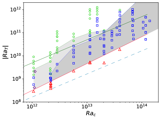
Figure 6: (Color online) Excerpt of fig. 3 emphasizing the transition from convection rolls (triangles) to fingers (circles) and staircases (squares) at large $Ra_{c}$ and $|Ra_{T}|$. The dashed line indicates $|\Lambda|=1/30$ and the lower straight solid line represents $\frac{1}{d}\sqrt{\kappa L_{f}/V}=1$, whereas the upper straight solid line is again at $|\Lambda|=1$.

IV.2 Transition from fingers to staircases

This transition is crossed by decreasing $|Ra_{T}|$ starting from large values at constant $Ra_{c}$ in fig. 3. We cannot hope for a quantitative prediction of the transition line of the same quality as in the previous section because the transition itself is not as sharp. However, the very existence of staircases at $|\Lambda|<1$ is noteworthy so that more qualitative considerations are also appropriate.

The mechanisms for staircase formation proposed in the past fall into several categories. There are those which postulate a lateral inhomogeneity Merryfield (2000) which likely exists in the oceans but which is not a plausible ingredient in a controlled laboratory environment. Another class of proposals is based on double diffusive effects in stably stratified media, such as the instability of internal gravity waves Stern (1969); Holyer (1981) or a stability criterion based on a Richardson number Kunze (1987). All these seem to be of little interest here since we observe staircases also in the unstably stratified case $|\Lambda|<1$.

A mechanism that turned out to be significant in recent simulations Sellmach et al. (2011); Yang et al. (2020) is an instability which appears Radko (2003) if the flux ratio has a minimum as a function of $|\Lambda|$. In that case, the difference between heat and salinity fluxes generates an unstably stratified zone within an otherwise stable background stratification which, so the original argument goes, leads to local overturning and ultimately a staircase. The argument may be modified for the present experiments by saying that $|\Lambda|$ becomes locally so small in some layer that large scale convection is preferred over fingers instead of expecting a convection roll as soon as $|\Lambda|<1$ in some layer. The flux ratio induced instability may therefore be a serious contender for explaining the staircase formation in the present experiments.

This hypothesis cannot be directly checked because the heat flux was not measured. In order to nonetheless obtain some information about the flux ratio, we will consider the situation prior to staircase formation in which fingers span the entire layer and in which the fingers obey the scalings reported in ref. Hage and Tilgner, 2010. A theoretical consideration allows us to narrow down the possible behaviour of the flux ratio in such a finger layer.

Double diffusive convection is described by the following set of equations for the fields of velocity $\bm{v}(\bm{r},t)$, concentration $c(\bm{r},t)$, temperature $T(\bm{r},t)$ and pressure $p(\bm{r},t)$:

$$\frac{\partial}{\partial t}\bm{v}+(\bm{v}\cdot\nabla)\bm{v}=-\frac{1}{\rho}\nabla p+\nu\nabla^{2}\bm{v}+g\alpha T\hat{\bm{z}}-g\beta c\hat{\bm{z}}$$ (10)

$$\nabla\cdot\bm{v}=0$$ (11)

$$\frac{\partial}{\partial t}T+\bm{v}\cdot\nabla T=\kappa\nabla^{2}T$$ (12)

$$\frac{\partial}{\partial t}c+\bm{v}\cdot\nabla c=D\nabla^{2}c$$ (13)

where $\hat{\bm{z}}$ denotes a unit vector in the vertical direction and the other variables are defined in section II. If we denote the average over space and time by angular brackets, we find by taking the scalar product of eq. (10) with $\bm{v}$ and subsequent averaging over space and time that

$$\epsilon=-g\beta\langle v_{z}c\rangle+g\alpha\langle v_{z}T\rangle$$ (14)

where $\epsilon$ is the dissipation defined as $\epsilon=\nu\sum_{i,j}\langle\left(\frac{\partial v_{j}}{\partial x_{i}}\right)^{2}\rangle$. If the entire layer is filled with uniform fingers, we may express the definition of the flux ratio $\gamma$ within the finger in terms of the above averages as

$$\gamma=\frac{\alpha\langle v_{z}T\rangle}{\beta\langle v_{z}c\rangle}.$$ (15)

With the help of the previous equation, $\gamma$ is given by

$$\gamma=1+\frac{\epsilon}{g\beta\langle v_{z}c\rangle}.$$ (16)

The denominator of the fraction is directly related to the measured Sherwood number by

$$\langle v_{z}c\rangle=-D\frac{\Delta c}{L}(Sh-1).$$ (17)

The dissipation $\epsilon$ on the other hand is not measured directly. However, the flow within fingers is essentially a laminar parallel shear flow so that the velocity profile is determined only by buoyancy and diffusion. For fingers of thickness $d$, the dissipation is given by $\epsilon=\nu K\langle v_{z}^{2}\rangle/d^{2}$ with some geometric factor $K$ which depends on the velocity profile within the fingers. For lamellar fingers with a sinusoidal profile and $v_{z}\propto\sin\left(\frac{\pi}{d}x\right)$, one finds $K=\pi^{2}$. For fingers of square cross section and $v_{z}\propto\sin\left(\frac{\pi}{d}x\right)\sin\left(\frac{\pi}{d}y\right)$ the factor $K$ is $K=2\pi^{2}$. The factor $K$ is larger if the velocity profile includes higher harmonics. In summary, one expects $K$ to be a modest multiple of $\pi^{2}$. Inserting the previous expressions into the formula for $\gamma$ leads to

$$\gamma=1-K\frac{Sc^{2}}{Ra_{c}}\frac{Re^{2}}{\left(\frac{d}{L}\right)^{2}(Sh-1)}$$ (18)

with the approximation $\langle v_{z}^{2}\rangle\approx\langle|\bm{v}|^{2}\rangle$ which is reasonable for finger convection. We next wish to obtain an expression for $\gamma$ in terms of the control parameters and have to eliminate the experimental observables $Re$, $d/L$ and $Sh$ in favor of $Ra_{c}$ and $Ra_{T}$. We will do so by invoking the scaling laws determined for pure finger convection Hage and Tilgner (2010):

$$\frac{d}{L}=0.95|Ra_{T}|^{-1/3}Ra_{c}^{1/9}$$ (19)

$$Re=10^{-6}|Ra_{T}|^{-1/2}Ra_{c}$$ (20)

$$Sh=0.016|Ra_{T}|^{-1/12}Ra_{c}^{4/9}$$ (21)

A theory put forward in ref. Yang, Verzicco, and Lohse, 2016 yields similar relationships, but as this theory also depends on empirically adjusted parameters, we prefer the scalings obtained from direct fits to the data. Inserting these into the expression for $\gamma$ finally yields

$$\gamma=1-69.25\times 10^{-12}Sc^{2}K|Ra_{T}|^{-1/4}Ra_{c}^{1/3}.$$ (22)

One can deduce from this equation that the scalings (19-21) cannot be valid for all $Ra_{c}$ and $|Ra_{T}|$ because $\gamma>0$ must hold. To see this, define the temperature deviation from the conduction profile $\theta$ as $\theta=T-T_{\rm{bottom}}+\Delta T\frac{z}{L}$. The equation of evolution for $\theta$ implied by eq. (12) is

$$\frac{\partial}{\partial t}\theta+\bm{v}\cdot\nabla\theta-\frac{\Delta T}{L}v_{z}=\kappa\nabla^{2}\theta$$ (23)

and $\theta$ must be zero on the boundaries. Multiplying this equation by $\theta$ and averaging over space and time yields

$$\frac{\Delta T}{L}\langle v_{z}\theta\rangle=\kappa\langle|\nabla\theta|^{2}\rangle.$$ (24)

Since $\langle v_{z}\theta\rangle=\langle v_{z}T\rangle$ and $\Delta T<0$, it follows that $\langle v_{z}T\rangle<0$. The analogous sequence of operations applied to the equation for $c$ yields $\langle v_{z}c\rangle<0$. As a consequence, $\gamma>0$.

The condition $\gamma>0$ constrains $Ra_{c}$ and $|Ra_{T}|$ in eq. (22) to

$$|Ra_{T}|\geq(69.25\times 10^{-12}Sc^{2}K)^{4}Ra_{c}^{4/3}$$ (25)

which is fulfilled for any reasonable choice of $K$ on the transition line between fingers and staircases in fig. 3. This means that the condition $\gamma>0$ does not determine when fingers cease to exist and staircases start to appear. We can therefore apply eq. (22) at the transition and transform it to

$$\gamma=1-69.25\times 10^{-12}Sc^{2}\left(\frac{Sc}{Pr}\right)^{1/4}K|\Lambda|^{-1/4}Ra_{c}^{1/12}.$$ (26)

It is frequently assumed that $\gamma$ is a function of $|\Lambda|$ alone and not of $Ra_{c}$ and $|Ra_{T}|$ independently. It is remarkable that, apart from a weak dependence on $Ra_{c}$ in $Ra_{c}^{1/12}$, eq. (26) nearly fulfills this property noting that it was obtained from the scalings eqs. (19-21) which themselves are the result of three independent fits to experimental data. The data from which (19-21) are deduced were obtained for approximately constant $Sc$ and $Pr$ so that the dependence on $Sc$ and $Pr$ in eq. (26) is meaningless. On the other hand, eq. (26) shows that $\gamma$ is a monotonically increasing function of $|\Lambda|$ whenever eqs. (19-21) are valid. There is therefore no indication of a minimum in the flux ratio as a function of $|\Lambda|$ and the flux ratio induced instability cannot be invoked as a mechanism for the staircase formation in the experiments reported here.

Having excluded all standard explanations for the existence of staircases, the question arises as to what actually caused them. A shear flow instability is not plausible either. The Reynolds number based on the finger thickness $Re_{d}=Re(d/L)$ is too small to generate an instability. $Re_{d}$ is less than 1.8 in all experiments. In the so called Kolmogorov flow, which is an infinitely extended parallel shear flow with a sinusoidal velocity profile, $Re_{d}$ would have to be at least $\sqrt{2}\pi$ to cause instability Green (1974).

Another scenario could be that at the combinations of $Ra_{c}$ and $Ra_{T}$ of staircases, the fingers never grow to full height if the voltage is switched on in the experiments while the temperature gradient is already established. A behavior of this type is observed in numerical simulations Singh and Srinivasan (2014) of fingers growing from an interface separating two homogeneous layers. In that case, fingers grow only to a certain finite length. A hint at the true instability mechanism may therefore be provided by how the flow evolves in time from initial conditions to finally form a staircase. The temporal evolution recorded in detail for $Ra_{c}=1.13\times 10^{13}$ and $|Ra_{T}|=1.14\times 10^{10}$ is shown in fig. 7. Starting from a uniform ion concentration and a linear temperature profile, fingers appeared next to the electrodes as the voltage was applied. Two fronts separating finger convection near each electrode from quiescent fluid in the center propagated away from the boundaries until they met in the middle of the cell. There was no mechanism at work to limit finger growth. The fingers then progressively thickened in a central layer until a single up and down flow were left over. Finally, the central layer increased somewhat to further reduce the height of the fingers in the bordering layers.

The increase of finger thickness reminds of the clustering of fingers which was found in numerical simulations Paparella and von Hardenberg (2012) which reproduced staircases in the sense of layers with alternating large and small gradients of temperature and salinity, but which did not show any layers with narrow fingers next to layers with broad structures. The explanation for these staircases again relies on a stable density stratification and is not easily transferred to the present problem.

The sequence of events in fig. 7 suggests that layering may be triggered by a random reduction of the stabilizing temperature gradient at some height. Assuming eq. 19 also holds locally in the form

$$d=0.95\left(\frac{g\alpha}{\kappa\nu}\right)^{-1/3}\left(\frac{g\beta}{D\nu}\right)^{1/9}\left(\frac{\Delta T}{L}\right)^{-1/3}\Delta c^{1/9},$$ (27)

a reduced temperature gradient leads to wider fingers at that height, which because of reduced friction increases the flow velocity inside the fingers, which in turn enhances the mixing and further reduces locally the temperature gradient to close a positive feedback loop. The local reduction of the temperature gradient must increase the temperature gradient in layers above and below the height at which the instability started, which suppresses transport in the upper and lower layers and saturates the instability. The example at $Ra_{c}=1.12\times 10^{13}$ and $|Ra_{T}|=4.97\times 10^{10}$, in fig. 4 would then simply show a case in which the unstable mode was prevented from growing to an amplitude at which the stabilizing temperature gradient at the center is reduced to the point that there is a single up and down flow in the central layer of the staircase. This scenario superficially fits the evolution of fingers in fig. 7, but future studies will have to determine whether this is a viable mechanism for staircase formation.

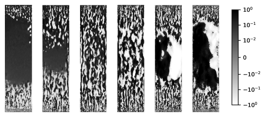
Figure 7: Time evolution in a cell of $40cm$ height at $Ra_{c}=1.13\times 10^{13}$ and $|Ra_{T}|=1.14\times 10^{10}$ at times (from left to right) $t=8min$, $14min$, $22min$, $115min$, $216min$ and $311min$ after the voltage was applied to the cell, and also after PIV particles were injected at the bottom. These particles rise and lead to a mean upward velocity at early times.

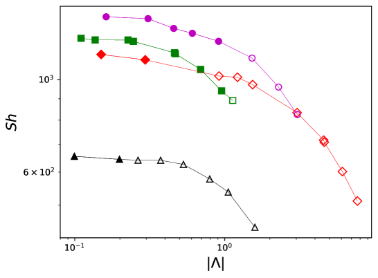
Figure 8: (Color online) $Sh$ as a function of $|\Lambda|$ for $Ra_{c}=1.06\times 10^{12}$ (triangles), $2.86\times 10^{12}$ (diamonds), $5.71\times 10^{12}$ (circles) and $2.04\times 10^{13}$ (squares). Filled and open symbols represent staircases and fingers crossing the whole cell, respectively.

V Transport

V.1 Transport through the cell

The previous section showed that the scalings (19-21) cannot hold at all $Ra_{c}$ and $Ra_{T}$ because eq. (26) is incompatible with the requirement $\gamma>0$ at large $Ra_{c}$. Another limit should exist for the validity of eq. (21) at large $|Ra_{T}|$. For $|\Lambda|=Pr/Sc$, or equivalently $|Ra_{T}|=Ra_{c}$, the system is linearly stable and in absence of any instability to finite amplitude perturbations, all motion must come to a stop and $Sh=1$. Eq. (21) however evaluates to $Sh=0.016Ra_{c}^{13/36}$ for $|Ra_{T}|=Ra_{c}$ which is far from 1. One therefore expects eq. (21) to lose validity if $|Ra_{T}|$ is large enough to be comparable with $Ra_{c}$. The different series of measurements carried out at constant $Ra_{c}$ by varying $|Ra_{T}|$ recognizable in fig. 3 probe the $|Ra_{T}|$ dependence of $Sh$. Fig. 8 shows $Sh$ for a few $Ra_{c}$ as a function of $|\Lambda|$. The parameter $\Lambda$ is proportional to $Ra_{T}$ if $Ra_{c}$, $Sc$ and $Pr$ are fixed. $Sh$ is weakly dependent on $|Ra_{T}|$ as predicted by eq. (21) for small $|\Lambda|$, but if $|\Lambda|$ is large enough, $Sh$ varies as expected more rapidly as a function of $|Ra_{T}|$. The full function $Sh(Ra_{c},|\Lambda|)$ is too complicated to be approximated by a simple analytical expression because the transition from slow to fast variation as a function of $|Ra_{T}|$ occurs at a different $|\Lambda|$ for different $Ra_{c}$. At any fixed $Ra_{c}$, the tangents to $Sh(|\Lambda|)$ at small and large $|\Lambda|$ intersect at some $|\Lambda|$. This intersection point marks the $|\Lambda|$ beyond which eq. (21) is certainly not valid any more. The question is whether it is always valid below that $|\Lambda|$. The region of parameter space in which $Sh$ varies slowly as a function of $|Ra_{T}|$ is delimited in fig. 3. Fig. 9 blindly applies eq. (21) to all measurements taken within this region irrespective of whether the flow is a single finger layer or a staircase. Within the scatter of the data, the Sherwood number for staircases does not allow one to tell staircases from fingers crossing the entire layer.

However, fig. 8 shows that eq. (21) cannot be the correct law for the Rayleigh number dependence of $Sh$ for the staircases. This follows from the fact that for example near $|\Lambda|=0.2$, the dependence of $Sh$ on $Ra_{c}$ is not monotonous in fig. 8. Fig. 8 also shows that there is no discontinuity in $Sh$ as the flow switches from a single finger layer to a staircase. If this transition occurs within the region in which $Sh$ depends little on $|Ra_{T}|$, as is the case for $Ra_{c}=1.06\times 10^{12}$ in fig. 8, one finds nearly identical $Sh$ for staircases and pure finger flows. This example supports the conclusion that a measurement of $Sh$ alone cannot distinguish fingers from staircases. This finding seems to contradict the statement in ref. Krishnamurti, 2003 that the Sherwood number depends inversely proportional to the number $n$ of finger layers. However, the behavior in $1/n$ is not seen for $n=1$ and $n=2$ in the data of ref. Krishnamurti, 2003 either, which contains data up to $n=8$, all obtained for $|\Lambda|>1$.

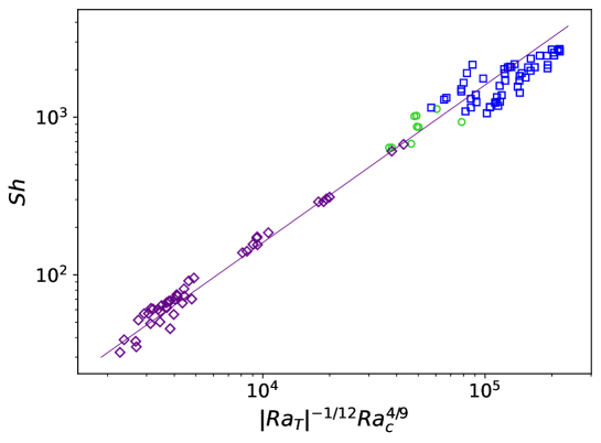
Figure 9: (Color online) The Sherwood number $Sh$ as a function of $|Ra_{T}|^{-1/12}Ra_{c}^{4/9}$ for all data from ref. Hage and Tilgner, 2010 (diamonds), and the fingers (circles) and staircases (squares) for which $Sh$ depends little on $|Ra_{T}|$ in the light shaded area in fig. 3. The solid line indicates $Sh=0.016|Ra_{T}|^{-1/12}Ra_{c}^{4/9}$.

V.2 Transport through finger layers

The goal of this section is to verify whether the ion transport through fingers in a staircase is the same as through fingers which extend from top to bottom boundaries, or whether a relation similar to eq. (21) also holds for fingers in staircases. For that purpose, one has to define chemical and thermal Rayleigh numbers $Ra_{T,f}$ and $Ra_{c,f}$ computed from the length of the fingers $L_{f}$ and the difference in ion concentration $\Delta c_{f}$ and temperature $\Delta T_{f}$ across the finger layer as

$$Ra_{T,f}=\frac{g\alpha\Delta T_{f}L_{f}^{3}}{\kappa\nu}~{}~{}~{},~{}~{}~{}Ra_{c,f}=\frac{g\beta\Delta c_{f}L_{f}^{3}}{D\nu}.$$ (28)

PIV measurements yield $L_{f}$ (see fig. 5) and the velocity within the central layer. The Peclet number based on this velocity, the height of the central layer and the ion diffusivity is in the range $10^{4}-10^{6}$ so that the central layer is expected to efficiently mix concentration and to annihilate any average concentration gradient in its interior. The concentration drop across the top and bottom finger layers must then be $\Delta c_{f}=\Delta c/2$ each. The analogous argument for temperature leading to $\Delta T_{f}=\Delta T/2$ is less compelling because the Peclet number for temperature is smaller. We will nonetheless assume $\Delta T_{f}=\Delta T/2$. To alleviate the impact of this assumption, we again restrict ourselves to the same data points as those retained in fig. 9 for which the temperature drop can be expected to only have a weak effect on the ion transport as predicted by eq. (21). Fig. 10 shows for this set of points that the finger Sherwood number $Sh_{f}$ defined as

$$Sh_{f}=\frac{j\,L_{f}}{z\,F\,D\,\Delta c_{f}}$$ (29)

is consistently larger for fingers in staircases than the Sherwood number for fingers crossing the entire cell. Note that the definitions of $Sh_{f}$, $Ra_{T,f}$ and $Ra_{c,f}$ reduce to their previously defined counter parts $Sh$, $Ra_{T}$ and $Ra_{c}$ if one sets $L_{f}=L$, $\Delta c_{f}=\Delta c$ and $\Delta T_{f}=\Delta T$ as is appropriate for fingers in a single finger layer. Apart from the prefactor, the scaling (21) is also a plausible summary of the Sherwood number measurements for fingers in staircases. A difference in prefactors is actually expected because of the difference in boundary conditions that apply at the tips of the different types of fingers.

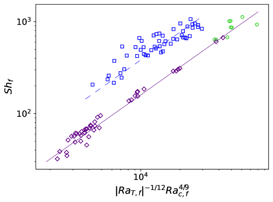
Figure 10: (Color online) The finger Sherwood number $Sh_{f}$ as a function of $|Ra_{T,f}|^{-1/12}Ra_{c,f}^{4/9}$ for all data from ref. Hage and Tilgner, 2010 (diamonds), and the fingers (circles) and staircases (squares) for which $Sh$ depends little on $|Ra_{T}|$ in the light shaded area in fig. 3. The solid line indicates $Sh_{f}=0.016|Ra_{T,f}|^{-1/12}Ra_{c,f}^{4/9}$, whereas the dashed line shows a power law with the same exponents but with a prefactor fitted to the staircases only, $Sh_{f}=0.0384|Ra_{T,f}|^{-1/12}Ra_{c,f}^{4/9}$.

VI Conclusion

The experiments reported here extend the parameter range covered by previous experiments with the same system. This allows us to pin down more precisely what determines the limit between finger convection and a single large scale convection layer. The insufficient diffusive transport of heat between neighboring fingers causes fingers to be replaced by standard convection flow.

Fingers may also give way to a staircase. The ion transport through the entire fluid layer varies continuously through the transition and the Sherwood does not allow one to distinguish a staircase from a single finger layer within the uncertainties of the data presented here. Despite the similarity in the global Sherwood number, the ion transport behaves clearly differently depending on whether ions are transported through fingers in a staircase or through fingers bridging the entire cell. The dependence of the Sherwood number on the Rayleigh numbers previously determined Hage and Tilgner (2010) for the latter type of fingers showed weak dependence on the thermal Rayleigh number. This scaling does not extrapolate properly to the parameters of linear onset of double diffusive convection, assuming that there indeed is no motion in the linearly stable system. The new experiments detected a deviation from the known scaling for sufficiently large density ratio.

The mechanism responsible for the formation of staircases, however, remains elusive. None of the previously proposed mechanisms provides us with a satisfactory explanation for the appearance of staircases in the experiments. It is known since ref. Hage and Tilgner, 2010 that finger convection occurs at $|\Lambda|<1$ even though the unstable stratification could just as well support global overturning. It then is not surprising any more to find staircases at $|\Lambda|<1$ as well. Field observations in the oceans have so far detected both salt fingers and staircases only for $|\Lambda|>1$. It will have to be decided in the future whether this is due to a lack of observations or whether there is a more fundamental difference between the oceanic staircases and laboratory experiments.

References

- Radko (2013) T. Radko, Double-Diffusive Convection (Cambridge University Press, 2013).
- Krishnamurti (2003) R. Krishnamurti, “Double-diffusive transport in laboratory thermohaline staircases,” J. Fluid Mech. 483, 287–314 (2003).
- Krishnamurti (2009) R. Krishnamurti, “Heat, salt and momentum transfer in a laboratory thermohaline staircase,” J. Fluid Mech. 638, 491–506 (2009).
- Hage and Tilgner (2010) E. Hage and A. Tilgner, “High Rayleigh number convection with double diffusive fingers,” Phys. Fluids 22, 076603 (2010).
- Kellner and Tilgner (2014) M. Kellner and A. Tilgner, “Transition to finger convection in double-diffusive convection,” Phys. Fluids 26, 094103 (2014).
- Goldstein, Chiang, and See (1990) R. J. Goldstein, H. D. Chiang, and D. L. See, “High-Rayleigh-number convection in a horizontal enclosure,” J. Fluid Mech. 213, 111–126 (1990).
- Kumar, Srivastava, and Karagadde (2018) V. Kumar, A. Srivastava, and S. Karagadde, “Compositional dependency of double-diffusive layers during binary alloy solidification: Full-field measurements and quantification,” Physics of Fluids 30, 113603 (2018).
- Radko (2020) T. Radko, “Suppression of internal waves by thermohaline staircases,” Journal of Fluid Mechanics 902, A14 (2020).
- Radko (2016) T. Radko, “Thermohaline layering in dynamically and diffusively stable shear flows,” Journal of Fluid Mechanics 805, 147–170 (2016).
- Brown and Radko (2019) J. M. Brown and T. Radko, “Initiation of diffusive layering by time-dependent shear,” Journal of Fluid Mechanics 858, 588–608 (2019).
- Yang et al. (2022) Y. Yang, R. Verzicco, D. Lohse, and C. Caulfield, “Layering and vertical transport in sheared double-diffusive convection in the diffusive regime,” Journal of Fluid Mechanics 933, A30 (2022).
- Ma and Peltier (2022) Y. Ma and W. Peltier, “Thermohaline staircase formation in the diffusive convection regime: a theory based upon stratified turbulence asymptotics,” Journal of Fluid Mechanics 931, R4 (2022).
- Radko (2003) T. Radko, “A mechanism for layer formation in a double-diffusive fluid,” Journal of Fluid Mechanics 497, 365–380 (2003).
- Sellmach et al. (2011) S. Sellmach, A. Traxler, P. Garaud, N. Brummell, and T. Radko, “Dynamics of fingering convection. part 2 the formation of thermohaline staircases,” Journal of Fluid Mechanics 677, 554–571 (2011).
- Traxler et al. (2011) A. Traxler, S. Stellmach, P. Garaud, T. Radko, and N. Brummel, “Dynamics of fingering convection. part 1 small-scale fluxes and large-scale instabilities,” Journal of Fluid Mechanics 677, 530–553 (2011).
- Ma and Peltier (2021) Y. Ma and W. R. Peltier, “Gamma instability in an inhomogeneous environment and salt-fingering staircase trapping: Determining the step size,” Phys. Rev. Fluids 6, 033903 (2021).
- Yang et al. (2020) Y. Yang, W. Chen, R. Verzicco, and D. Lohse, “Multiple states and transport properties of double-diffusive convection turbulence,” Proc. Nat. Acad. Sci. 117, 14676–14681 (2020).
- Radko (2014) T. Radko, “Applicability and failure of the flux-gradient laws in double-diffusive convection,” Journal of Fluid Mechanics 750, 33–72 (2014).
- Radko (2019) T. Radko, “Thermohaline layering on the microscale,” Journal of Fluid Mechanics 862, 672–695 (2019).
- Probstein (1995) R. F. Probstein, Physicochemical Hydrodynamics (John Wiley & Sons, New York, 1995).
- Merryfield (2000) W. J. Merryfield, “Origin of thermohaline staircases,” Jornal of Physical Oceanography 30, 1046–1068 (2000).
- Stern (1969) M. E. Stern, “Collective instability of salt fingers,” J. Fluid Mech. 35, 209–218 (1969).
- Holyer (1981) J. Y. Holyer, “On the collective instability of salt fingers,” J. Fluid Mech. 110 (1981).
- Kunze (1987) E. Kunze, “Limits on growing, finite-length salt fingers: A Richardson number constraint,” Journal of Marine Research 45, 533–556 (1987).
- Yang, Verzicco, and Lohse (2016) Y. Yang, R. Verzicco, and D. Lohse, “Scaling laws and flow structures of double diffusive convection in the finger regime,” Journal of Fluid Mechanics 802, 667–689 (2016).
- Green (1974) J. S. A. Green, “Two-dimensional turbulence near the viscous limit,” J. Fluid Mech. 62, 273–287 (1974).
- Singh and Srinivasan (2014) O. P. Singh and J. Srinivasan, “Effect of Rayleigh numbers on the evolution of double-diffusive salt fingers,” Physics of Fluids 26, 062104 (2014).
- Paparella and von Hardenberg (2012) F. Paparella and J. von Hardenberg, “Clustering of salt fingers in double-diffusive convection leads to staircaselike stratification,” Phys. Rev. Lett. 109, 014502 (2012).