WaveBound: Dynamic Error Bounds for Stable Time Series Forecasting

Abstract

Time series forecasting has become a critical task due to its high practicality in real-world applications such as traffic, energy consumption, economics and finance, and disease analysis. Recent deep-learning-based approaches have shown remarkable success in time series forecasting. Nonetheless, due to the dynamics of time series data, deep networks still suffer from unstable training and overfitting. Inconsistent patterns appearing in real-world data lead the model to be biased to a particular pattern, thus limiting the generalization. In this work, we introduce the dynamic error bounds on training loss to address the overfitting issue in time series forecasting. Consequently, we propose a regularization method called WaveBound which estimates the adequate error bounds of training loss for each time step and feature at each iteration. By allowing the model to focus less on unpredictable data, WaveBound stabilizes the training process, thus significantly improving generalization. With the extensive experiments, we show that WaveBound consistently improves upon the existing models in large margins, including the state-of-the-art model.

1 Introduction

Time series forecasting has gained a lot of attention due to its high practicality in real-world applications such as traffic [1], energy consumption [2], economics and finance [3], and disease analysis [4]. Recent deep-learning-based approaches, particularly transformer-based methods [5, 6, 7, 8, 9], have shown remarkable success in time series forecasting. Nevertheless, inconsistent patterns and unpredictable behaviors in real data enforce the models to fit in patterns, even for the cases of unpredictable incident, and induce the unstable training. In unpredictable cases, the model does not neglect them in training, but rather receives a huge penalty (i.e., training loss). Ideally, small magnitudes of training loss should be presented for unpredictable patterns. This implies the need for proper regularization of the forecasting models in time series forecasting.

Recently, Ishida et al. [10] claimed that zero training loss introduces a high bias in training, hence leading to an overconfident model and a decrease in generalization. To remedy this issue, they propose a simple regularization called flooding and explicitly prevent the training loss from decreasing below a small constant threshold called the flood level. In this work, we also focus on the drawbacks of zero training loss in time series forecasting. In time series forecasting, the model is enforced to fit to an inevitably appearing unpredictable pattern which mostly generates a tremendous error. However, the original flooding is not applicable to time series forecasting mainly due to the following two main reasons. (i) Unlike image classification, time series forecasting requires the vector output of the size of the prediction length times the number of features. In this case, the original flooding considers the average training loss without dealing with each time step and feature individually. (ii) In time series data, error bounds should be dynamically changed for different patterns. Intuitively, a higher error should be tolerated for unpredictable patterns.

To properly address the overfitting issue in time series forecasting, the difficulty of prediction, i.e., how unpredictable the current label is, should be measured in the training procedure. To this end, we introduce the target network updated with an exponential moving average of the original network, i.e., source network. At each iteration, the target network can guide a reasonable level of training loss to the source network — the larger the error of the target network, the more unpredictable the pattern. In current studies, a slow-moving average target network is commonly used to produce stable targets in the self-supervised setting [11, 12]. By using the training loss of the target network for our lower bound, we derive a novel regularization method called WaveBound which faithfully estimates the error bounds for each time step and feature. By dynamically adjusting the error bounds, our regularization prevents the model from overly fitting to a certain pattern and further improves generalization. Figure 1 shows the conceptual difference between the original flooding and our WaveBound method. The originally proposed flooding determines the direction of the update step for all points by comparing the average loss and its flood level. In contrast, WaveBound individually decides the direction of the update step for each point by using the dynamic error bound of the training loss. The difference between these methods is further discussed in Section 3. Our main contributions are threefold:

• We propose a simple yet effective regularization method called WaveBound that dynamically provides the error bounds of training loss in time series forecasting.

• We show that our proposed regularization method consistently improves upon the existing state-of-the-art time series forecasting model on six real-world benchmarks.

• By conducting extensive experiments, we verify the significance of adjusting the error bounds for each time step, feature, and pattern, thus addressing the overfitting issue in time series forecasting.

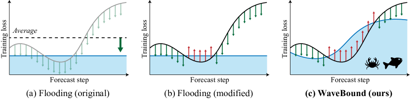
Figure 1: The conceptual examples for different methods. (a) The original flooding provides the lower bound of the average loss, rather than considering each time step and feature individually. (b) Even if the lower bounds of training loss are provided for each time step and feature, the bound of constant value cannot reflect the nature of time series forecasting. (c) Our proposed WaveBound method provides the lower bound of the training loss for each time step and feature. This lower bound is dynamically adjusted to give a tighter error bound during the training process.

2 Preliminary

2.1 Time Series Forecasting

We consider the rolling forecasting setting with a fixed window size [5, 6, 7]. The aim of time series forecasting is to learn a forecaster $g:\mathbb{R}^{L\times K}\rightarrow\mathbb{R}^{M\times K}$ which predicts the future series $y^{t}=\{z_{t+1},z_{t+2},...,z_{t+M}:z_{i}\in\mathbb{R}^{K}\}$ given the past series $x^{t}=\{z_{t-L+1},z_{t-L+2},...,z_{t}:z_{i}\in\mathbb{R}^{K}\}$ at time $t$ where $K$ is the feature dimension and $L$ and $M$ are the input length and output length, respectively. We mainly address the error bounding in the multivariate regression problem where the input series $x$ and output series $y$ jointly come from the underlying density $p(x,y)$. For a given loss function $\ell$, the risk of $g$ is $R(g)\coloneqq\mathbb{E}_{(x,y)\sim p(x,y)}\left[\ell(g(x),y)\right]$. Since we cannot directly access the distribution $p$, we instead minimize its empirical version $\hat{R}(g)\coloneqq\frac{1}{N}\sum_{i=1}^{N}\ell(g(x_{i}),y_{i})$ using training data $\mathcal{X}\coloneqq\{(x_{i},y_{i})\}_{i=1}^{N}$. In the analysis, we assume that the errors are independent and identically distributed. We mainly consider using the mean squared error (MSE) loss, which is widely used as an objective function in recent time series forecasting models [5, 6, 7]. Then, the risk can be rewritten as the sum of the risk at each prediction step and feature:

$$R(g)= \mathbb{E}_{(u,v)\sim p(u,v)}\left[\frac{1}{MK}||g(u)-v||^{2}\right]=\frac{1}{MK}\sum_{j,k}R_{jk}(g),$$ (1)

$$\hat{R}(g)= \frac{1}{NMK}\sum_{i=1}^{N}||g(x_{i})-y_{i}||^{2}=\frac{1}{MK}\sum_{j,k}\hat{R}_{jk}(g),$$

where $R_{jk}(g)\coloneqq\mathbb{E}_{(u,v)\sim p(u,v)}\left[||g_{jk}(u)-v_{jk}||^{2}\right]$ and $\hat{R}_{jk}(g)\coloneqq\frac{1}{N}\sum_{i=1}^{N}||g_{jk}(x_{i})-(y_{i})_{jk}||^{2}$.

2.2 Flooding

To address the overfitting problem, Ishida et al. [10] suggested flooding, which restricts the training loss to stay above a certain constant. Given the empirical risk $\hat{R}$ and the manually searched lower bound $b$, called the flood level, we instead minimize the flooded empirical risk, which is defined as

$$\hat{R}^{fl}(g)=|\hat{R}(g)-b|+b.$$ (2)

The gradient update of the flooded empirical risk with respect to the model parameters is performed as that of the empirical risk if $\hat{R}(g)>b$ and is otherwise performed in the opposite direction. The flooded empirical risk estimator is known to provide a better approximation of the risk than the empirical risk estimator in terms of MSE if the risk is greater than $b$.

For the mini-batched optimization, a gradient update of the flooded empirical risk is performed with respect to the mini-batch. Let $\hat{R}_{t}(g)$ denote the empirical risk with respect to the $t$-th mini-batch for $t\in\{1,2,...,T\}$. Then, by Jensen’s inequality,

$$\hat{R}^{fl}(g)\leq\frac{1}{T}\sum_{t=1}^{T}(|\hat{R}_{t}(g)-b|+b).$$ (3)

Therefore, the mini-batched optimization minimizes the upper bound of the flooded empirical risk.

3 Method

In this section, we propose a novel regularization called WaveBound which is specially-designed for time series forecasting. We first deal with the drawbacks of applying original flooding to time series forecasting and then introduce a more desirable form of regularization.

3.1 Flooding in Time Series Forecasting

We first discuss how the original flooding may not effectively work for the time series forecasting problem. We start with rewriting Equation (2) using the risks at each prediction step and feature:

$$\hat{R}^{fl}(g)=\left|\hat{R}(g)-b\right|+b=\left|\left(\frac{1}{MK}\sum_{j,k}\hat{R}_{jk}(g)\right)-b\right|+b.$$ (4)

Flooded empirical risk constrains the lower bound of the average of the empirical risk for all prediction steps and features by a constant value of $b$. However, for the multivariate regression model, this regularization does not independently bound each $\hat{R}_{jk}(g)$. As a result, the regularization effect is concentrated on output variables where $\hat{R}_{jk}(g)$ greatly varies in training.

In this circumstance, the modified version of flooding can be explored by considering the individual training loss for each time step and feature. This can be done by subtracting the flood level $b$ for each time step and feature as follows:

$$\hat{R}^{const}(g)=\frac{1}{MK}\sum_{j,k}\Big{(}|\hat{R}_{jk}(g)-b|+b\Big{)}.$$ (5)

For the remainder of this study, we denote this version of flooding as constant flooding. Compared to the original flooding that considers the average of the whole training loss, constant flooding individually constrains the lower bound of the training loss at each time step and feature by the value of $b$.

Nonetheless, it still fails to consider different difficulties of predictions for different mini-batches. For constant flooding, it is challenging to properly minimize the variants of empirical risk in the batch-wise training process. As in Equation 3, the mini-batched optimization minimizes the upper bound of the flooded empirical risk. The problem is that the inequality becomes less tight as each flooded risk term $\hat{R}_{t}(g)-b$ for $t\in\{1,2,...,T\}$ differs significantly. Since the time series data typically contains lots of unpredictable noise, this happens frequently as the loss of each batch highly varies. To ensure the tightness of the inequality, the bound for $\hat{R}_{t}(g)$ should be adaptively chosen for each batch.

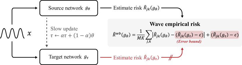
Figure 2: Our proposed WaveBound method provides the dynamic error bounds of the training loss for each time step and feature using the target network. The target network $g_{\tau}$ is updated with the EMA of the source network $g_{\theta}$. At $j$-th time step and $k$-th feature, the training loss is bounded by our estimated error bound $\hat{R}_{jk}(g_{\tau})-\epsilon$, i.e., the gradient ascent is performed instead of the gradient descent when the training loss is below the error bound.

3.2 WaveBound

As previously mentioned, to properly bound the empirical risk in time series forecasting, the regularization method should be considered with the following conditions: (i) The regularization should consider the empirical risk for each time step and feature individually. (ii) For different patterns, i.e., mini-batches, different error bounds should be searched in the batch-wise training process. To handle this, we find the error bound for each time step and feature and dynamically adjust it at each iteration. Since manually searching different bounds for each time step and feature at every iteration is impractical, we estimate the error bounds for different predictions using the exponential moving average (EMA) model  [13].

Concretely, two networks are employed throughout the training phase: the source network $g_{\theta}$ and target network $g_{\tau}$ which have the same architecture, but different weights $\theta$ and $\tau$, respectively. The target network estimates the proper lower bounds of errors for the predictions of the source network, and its weights are updated with the exponential moving average of the weights of the source network:

$$\tau\leftarrow\alpha\tau+(1-\alpha)\theta,$$ (6)

where $\alpha\in\left[0,1\right]$ is a target decay rate. On the other hands, the source network updates their weights $\theta$ using the gradient descent update in the direction of the gradient of wave empirical risk $\hat{R}^{wb}(g_{\theta})$ which is defined as

$$\hat{R}^{wb}(g_{\theta}) =\frac{1}{MK}\sum_{j,k}\hat{R}^{wb}_{jk}(g_{\theta}),$$ (7)

$$\hat{R}^{wb}_{jk}(g_{\theta}) =\left|\hat{R}_{jk}(g_{\theta})-(\hat{R}_{jk}(g_{\tau})-\epsilon)\right|+(\hat{R}_{jk}(g_{\tau})-\epsilon),$$

where $\epsilon$ is a hyperparameter indicating how far the error bound of the source network can be from the error of the target network. Intuitively, the target network guides the lower bound of the training loss for each time step and feature to prevent the source network from training towards a loss lower than that bound, i.e., overfitting to a certain pattern. As the exponential moving average model is known to have the effect of ensembling the source networks and memorizing training data visible in earlier iterations [13], the target network can robustly estimate the error bound of the source network against the instability mostly caused by noisy input data. Figure 2 shows how the source network and the target network perform in our WaveBound method. A summary of WaveBound is provided in Appendix B.

Mini-batched optimization. For $t\in\{1,2,...,T\}$, let $(\hat{R}^{wb}_{t})_{jk}(g)$ and $(\hat{R}_{t})_{jk}(g)$ denote the wave empirical risk and the empirical risk at $j$-th step and $k$-th feature relative to the $t$-th mini-batch, respectively. Given the target network $g^{\ast}$, by Jensen’s inequality,

$$\hat{R}^{wb}_{jk}(g)\leq\frac{1}{T}\sum_{t=1}^{T}\left(\left|(\hat{R}_{t})_{jk}(g)-(\hat{R}_{t})_{jk}(g^{\ast})+\epsilon\right|+(\hat{R}_{t})_{jk}(g^{\ast})-\epsilon\right)=\frac{1}{T}\sum_{t=1}^{T}(\hat{R}^{wb}_{t})_{jk}(g).$$ (8)

Therefore, the mini-batched optimization minimizes the upper bound of wave empirical risk. Note that if $g$ is close to $g^{\ast}$, the values of $(\hat{R}_{t})_{jk}(g)-(\hat{R}_{t})_{jk}(g^{\ast})+\epsilon$ are similar across mini-batches, which gives a tight bound in Jensen’s inequality. We expect the EMA update to work so that this condition is met, giving a tight upper bound for the wave empirical risk in the mini-batched optimization.

MSE reduction. We show that the MSE of our suggested wave empirical risk estimator can be smaller than that of the empirical risk estimator given an appropriate $\epsilon$. thmuniverse Fix measurable functions $g$ and $g^{\ast}$. Let $I\coloneqq\{(i,j):i=1,2,...,M,j=1,2,...,K\}$, and let $J(\mathcal{X})\coloneqq\{(i,j)\in I:\hat{R}_{ij}(g)<\hat{R}_{ij}(g^{\ast})-\epsilon\}$. If the following two conditions hold:

1. $\forall(i,j),(k,l)\in I\>\text{such that}\>(i,j)\neq(k,l),\;\hat{R}_{ij}(g)-\hat{R}_{ij}(g^{\ast})\perp\hat{R}_{kl}(g)$

2. $\hat{R}_{ij}(g^{\ast})<R_{ij}(g)+\epsilon$ for all $(i,j)\in J(\mathcal{X})$ almost surely,

then $\text{MSE}(\hat{R}(g))\geq\text{MSE}(\hat{R}^{wb}(g))$. Given the condition (a), if we have $0<\alpha$ such that $\alpha<R_{ij}(g)-\hat{R}_{ij}(g^{\ast})+\epsilon$ for all $(i,j)\in J(\mathcal{X})$ almost surely, then

$$\text{MSE}(\hat{R}(g))-\text{MSE}(\hat{R}^{wb}(g))\geq 4\alpha^{2}\sum_{(i,j)\in I}\Pr[\alpha<\hat{R}_{ij}(g^{\ast})-\hat{R}_{ij}(g)-\epsilon].$$ (9)

Proof.

Please see Appendix A. ∎

Intuitively, Theorem 3.2 states that the MSE of the empirical risk estimator can be reduced when the following conditions hold: (i) The network $g^{\ast}$ has sufficient expressive power so that the loss difference between $g$ and $g^{\ast}$ at each output variable is unrelated to the loss at the other output variables in $g$. (ii) $\hat{R}_{ij}(g^{\ast})-\epsilon$ likely lies in between $\hat{R}_{ij}(g)$ and $R_{ij}(g)$. It is preferable to have $g^{\ast}$ as the EMA model of $g$ since the training loss of the EMA model cannot be readily below the test loss of the model. Then, $\epsilon$ can be chosen as a fixed small value so that the training loss of the source model at each output variable can be closely bounded below by the test loss at that variable.

4 Experiments

4.1 WaveBound with Forecasting Models

Table 1: The results of WaveBound in the multivariate setting. All results are averaged over 3 trials.

Models Autoformer [5] Pyraformer [6] Informer [7] LSTNet [14] Origin w/ Ours Origin w/ Ours Origin w/ Ours Origin w/ Ours Metric MSE MAE MSE MAE MSE MAE MSE MAE MSE MAE MSE MAE MSE MAE MSE MAE ETTm2 96 0.262 0.326 0.204 0.285 0.363 0.451 0.281 0.386 0.376 0.477 0.334 0.429 0.455 0.511 0.268 0.368 192 0.284 0.342 0.265 0.322 0.708 0.648 0.624 0.599 0.751 0.672 0.698 0.631 0.706 0.660 0.464 0.508 336 0.338 0.374 0.320 0.356 1.130 0.846 1.072 0.829 1.440 0.917 1.087 0.845 1.161 0.868 0.781 0.695 720 0.446 0.435 0.413 0.408 2.995 1.386 1.917 1.119 3.897 1.498 2.984 1.411 3.288 1.494 2.312 1.239 ECL 96 0.202 0.317 0.176 0.288 0.256 0.360 0.241 0.345 0.335 0.417 0.289 0.378 0.268 0.366 0.185 0.291 192 0.235 0.340 0.205 0.317 0.272 0.378 0.256 0.360 0.341 0.426 0.298 0.388 0.277 0.375 0.197 0.304 336 0.247 0.351 0.217 0.327 0.278 0.383 0.269 0.371 0.369 0.448 0.305 0.394 0.284 0.382 0.217 0.326 720 0.270 0.371 0.260 0.359 0.291 0.385 0.283 0.377 0.396 0.457 0.311 0.398 0.316 0.404 0.250 0.350 Exchange 96 0.153 0.285 0.146 0.274 0.604 0.624 0.615 0.627 0.979 0.791 0.878 0.765 0.483 0.518 0.357 0.432 192 0.297 0.397 0.262 0.373 0.982 0.806 0.953 0.797 1.147 0.854 1.136 0.859 0.706 0.646 0.621 0.593 336 0.438 0.490 0.425 0.483 1.264 0.934 1.263 0.944 1.592 1.014 1.461 0.992 1.055 0.800 0.837 0.691 720 1.207 0.860 1.088 0.810 1.663 1.051 1.562 1.016 2.540 1.306 2.496 1.294 2.198 1.127 1.374 0.894 Traffic 96 0.645 0.399 0.596 0.352 0.635 0.364 0.622 0.341 0.731 0.412 0.671 0.364 0.735 0.446 0.587 0.356 192 0.644 0.407 0.607 0.370 0.658 0.376 0.646 0.355 0.751 0.422 0.666 0.360 0.750 0.446 0.595 0.365 336 0.625 0.390 0.603 0.361 0.668 0.377 0.653 0.355 0.822 0.465 0.709 0.387 0.778 0.455 0.623 0.378 720 0.650 0.398 0.642 0.383 0.698 0.390 0.672 0.364 0.957 0.539 0.764 0.421 0.815 0.470 0.648 0.383 Weather 96 0.294 0.355 0.227 0.296 0.235 0.321 0.193 0.272 0.378 0.428 0.355 0.415 0.237 0.310 0.202 0.275 192 0.308 0.368 0.283 0.340 0.340 0.415 0.306 0.372 0.462 0.467 0.424 0.448 0.277 0.343 0.254 0.316 336 0.364 0.396 0.335 0.370 0.453 0.484 0.403 0.441 0.575 0.535 0.506 0.484 0.326 0.378 0.309 0.358 720 0.426 0.433 0.401 0.411 0.599 0.563 0.535 0.519 1.024 0.751 0.972 0.712 0.412 0.431 0.398 0.415 ILI 24 3.468 1.299 3.118 1.200 4.822 1.489 4.679 1.459 5.356 1.590 4.947 1.494 7.934 2.091 6.331 1.816 36 3.441 1.273 3.310 1.240 4.831 1.479 4.763 1.483 5.131 1.569 5.027 1.537 8.793 2.214 6.560 1.848 48 3.086 1.184 2.927 1.128 4.789 1.465 4.524 1.439 5.150 1.564 4.920 1.514 7.968 2.068 6.154 1.779 60 2.843 1.136 2.785 1.116 4.876 1.495 4.573 1.465 5.407 1.604 5.013 1.528 7.387 1.984 6.119 1.758

Table 2: The results of WaveBound in the univariate setting. All results are averaged over 3 trials.

Models Autoformer [5] Pyraformer [6] Informer [7] N-BEATS [15] Origin w/ Ours Origin w/ Ours Origin w/ Ours Origin w/ Ours Metric MSE MAE MSE MAE MSE MAE MSE MAE MSE MAE MSE MAE MSE MAE MSE MAE ETTm2 96 0.098 0.239 0.085 0.221 0.078 0.209 0.070 0.197 0.085 0.224 0.081 0.218 0.073 0.198 0.067 0.188 192 0.130 0.277 0.116 0.262 0.114 0.257 0.110 0.256 0.122 0.273 0.118 0.270 0.107 0.246 0.103 0.241 336 0.162 0.311 0.143 0.293 0.178 0.325 0.153 0.306 0.153 0.304 0.148 0.305 0.163 0.310 0.135 0.284 720 0.194 0.344 0.188 0.338 0.198 0.351 0.169 0.329 0.196 0.351 0.189 0.349 0.263 0.402 0.188 0.340 ECL 96 0.462 0.502 0.447 0.496 0.240 0.351 0.229 0.347 0.266 0.371 0.261 0.369 0.304 0.382 0.298 0.378 192 0.557 0.565 0.515 0.538 0.262 0.367 0.253 0.365 0.283 0.385 0.281 0.383 0.323 0.396 0.322 0.395 336 0.613 0.593 0.531 0.543 0.285 0.386 0.283 0.386 0.338 0.428 0.332 0.426 0.385 0.430 0.369 0.422 720 0.691 0.632 0.604 0.591 0.309 0.411 0.307 0.415 0.631 0.612 0.378 0.463 0.462 0.487 0.433 0.473

In this section, we evaluate our WaveBound method on real-world benchmarks using various time series forecasting models, including the state-of-the-art models.

Baselines. Since our method can be easily applied to deep-learning-based forecasting models, we evaluate our regularization adopted by several baselines including the state-of-the-art method. For the multivariate setting, we select Autoformer [5], Pyraformer [6], Informer [7], LSTNet [14], and TCN [16]. For the univariate setting, we additionally include N-BEATS [15] for the baseline.

Datasets. We examine the performance of forecasting models in six real-world benchmarks. (1) The Electricity Transformer Temperature (ETT) [7] dataset contains two years of data from two separate counties in China with intervals of 1-hour level (ETTh1, ETTh2) and 15 minutes level (ETTm1, ETTm2) collected from electricity transformers. Each time step contains an oil temperature and 6 additional features. (2) The Electricity (ECL)  dataset comprises 2 years of hourly electricity consumption of 321 clients. (3) The Exchange [14] dataset provides a collection of eight distinct countries on a daily basis. (4) The Traffic  dataset contains hourly statistics of various sensors in San Francisco Bay provided by the California Department of Transportation. Road occupancy rate is expressed as a real number between 0 and 1. (5) The Weather  dataset records 4 years of data (2010-2013) of 21 meteorological indicators collected at around 1,600 landmarks in the United States. (6) The ILI  dataset contains data from the Centers for Disease Control and Prevention’s weekly reported influenza-like illness patients from 2002 to 2021, which describes the ratio of patients seen with ILI to the overall number of patients. As in Autoformer [5], we set $L=36$ and $M\in\{24,36,48,60\}$ for the ILI dataset, and set $L=96$ and $M\in\{96,192,336,720\}$ for the other datasets. We split each dataset into train/validation/test as follows: 6:2:2 ratio for the ETT dataset and 7:1:2 ratio for the rest.

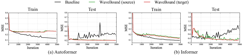
Figure 3: The training curves of models with and without WaveBound on the ETTm2 dataset. Without WaveBound, the training loss of both models decreases, but the test loss increases (See black lines), which indicates that both models tend to overfit at the training data. In contrast, the test loss of models with WaveBound continue to decrease after learning for even more epochs.

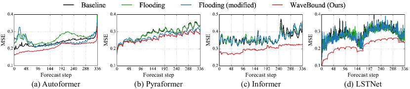
Figure 4: The test error of models trained with different regularization methods on the ECL dataset. Compared with original flooding and constant flooding, the test error of WaveBound is consistently lower at all time steps, which indicates that our method successfully improves generalization regardless of the range of predictions.

Multivariate Results. Table 1 shows the performance of our method in terms of mean squared error (MSE) and mean absolute error (MAE) in the multivariate setting. We can observe that our method consistently shows improvements for various forecasting models including the state-of-the-art methods. Notably, WaveBound improves both MAE and MSE of Autoformer on the ETTm2 dataset by 22.13% $(0.262\rightarrow 0.204)$ in MSE and 12.57% $(0.326\rightarrow 0.285)$ in MAE when $M=96$. In particular, the performance is improved by 41.10% $(0.455\rightarrow 0.268)$ in MSE and 27.98% $(0.511\rightarrow 0.368)$ in MAE for LSTNet. For long-term ETTm2 forecasting settings $(M=720)$, WaveBound improves the performance of Autoformer by 7.39% $(0.446\rightarrow 0.413)$ in MSE and 6.20% $(0.435\rightarrow 0.408)$ in MAE. In all experiments, our method consistently shows performance improvements with various forecasting models. The results of full baselines and benchmarks are reported in Appendix D.

Univariate Results. WaveBound also shows superior results in the univariate setting, as reported in Table 2. In particular, for N-BEATS, which is designed especially for univariate time series forecasting, our method improves the performance on the ETTm2 dataset by 8.22% $(0.073\rightarrow 0.067)$ in MSE and 5.05% $(0.198\rightarrow 0.188)$ in MAE, when $M=96$. For the ECL dataset, Informer with WaveBound shows improvements of 40.10% $(0.631\rightarrow 0.378)$ in MSE and 24.35% $(0.612\rightarrow 0.463)$ in MAE when $M=720$. The results of the full baselines and benchmarks are reported in Appendix D.

Generalization Gaps. To identify overfitting, the generalization gap, which is the difference between the training loss and the test loss, can be examined. To verify that our regularization truly prevents overfitting, we depict both the training loss and test loss for models with and without WaveBound in Figure 3. Without WaveBound, the test loss starts to increase abruptly, showing a high generalization gap. In contrast, when using WaveBound, we can observe that the test loss continued to decrease, which indicates that WaveBound successfully addresses overfitting in time series forecasting.

4.2 Significance of Dynamically Adjusting Error Bounds

In WaveBound, the error bound is dynamically adjusted at each iteration for each time step and feature. To validate the significance of such dynamics, we compare our WaveBound with the original flooding and constant flooding which use the constant values for flood levels, as introduced in Section 3.

Table 3: The results of variants of flooding regularization on the ECL dataset. We compare the forecasting accuracy when training the source network using different surrogates to empirical risk. All results are averaged over 3 trials and the constant value $b$ is faithfully searched in $\{0.00,0.02,0.04,...0.40\}$.

Method	Estimated risk (w/o constant)		Autoformer		Pyraformer		Informer		LSTNet
			96	336	96	336	96	336	96	336
Base model	$\hat{R}(g)$	MSE	0.202	0.247	0.256	0.278	0.335	0.369	0.268	0.284
		MAE	0.317	0.351	0.360	0.383	0.417	0.448	0.366	0.382
Flooding [10]	$\lvert\hat{R}(g)-b\rvert$	MSE	0.194	0.247	0.257	0.277	0.335	0.368	0.268	0.284
		MAE	0.309	0.351	0.360	0.382	0.416	0.447	0.366	0.381
Constant flooding	$\frac{1}{MK}\sum\limits_{j,k}\lvert\hat{R}_{jk}(g)-b\rvert$	MSE	0.198	0.247	0.257	0.277	0.333	0.369	0.268	0.284
		MAE	0.314	0.351	0.360	0.382	0.415	0.448	0.366	0.382
WaveBound (Avg.)	$\lvert\hat{R}(g)-\hat{R}(g^{\ast})+\epsilon\rvert$	MSE	0.194	0.221	0.248	0.288	0.302	0.322	0.208	0.246
		MAE	0.309	0.331	0.352	0.388	0.388	0.407	0.314	0.356
WaveBound (Indiv.)	$\frac{1}{MK}\sum\limits_{j,k}\lvert\hat{R}_{jk}(g)-\hat{R}_{jk}(g^{\ast})+\epsilon\rvert$	MSE	0.176	0.217	0.241	0.269	0.289	0.305	0.185	0.217
		MAE	0.288	0.327	0.345	0.371	0.378	0.394	0.291	0.326

Table 3 compares the performance of variants of flooding regularization with different surrogates to empirical risk. The original flooding bounds the empirical risk by a constant while constant flooding bounds the risk at each feature and time step independently. We searched the flood level $b$ for the regularization methods with constant value $b$ in space of $\{0.00,0.02,0.04,...0.40\}$. As we expected, we cannot achieve the improvements when using a fixed constant value. The models trained by individually bounding the error in each output variable outperform other baselines by a large margin, which concretely shows the effectiveness of our proposed WaveBound method. The test error of different methods for each time step is depicted in Figure 4. For all time steps, WaveBound shows an improved generalization compared to original flooding and constant flooding, which highlights the significance of adjusting the error bounds in time series forecasting.

4.3 Flatness of Loss Landscapes

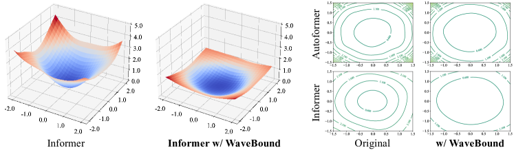
Figure 5: The loss landscapes of Autoformer and Informer trained with and without our WaveBound on the ETTh1 dataset. WaveBound flattens the loss landscapes for both models, improving the generalization of models.

The visualization of loss landscapes [17] is introduced to evaluate how the model adequately generalizes. It is known that the flatter the loss landscapes of the model, the better the robustness and generalization [18, 19]. In this section, we depict the loss landscapes of models trained with and without WaveBound. Figure 5 shows the loss landscapes of Autoformer and Informer. We visualize the loss landscapes using filter normalization [17] and evaluate the MSE for every model for a fair comparison. We can observe that the model with WaveBound shows smoother loss landscapes compared to that of the original model. In other words, WaveBound flattens the loss landscapes of time series forecasting models and stabilizes the training.

5 Related Work

Time series forecasting. For time series forecasting tasks, various approaches have been proposed based on different principles. Statistical approaches can provide interpretability as well as a theoretical guarantee. Auto-regressive Integrated Moving Average  [20] and Prophet [21] are the most representative methods for statistical approaches. Another important class of time series forecasting is the state space models [22, 23] (SSMs). SSMs incorporate structural assumptions into the model and learn latent dynamics of the time series data. However, due to its superior results in long-range forecasting, deep-learning-based approaches are mainly considered as the prominent solution for time series forecasting. To model the temporal dependencies in time series data, recurrent neural networks (RNN) [24, 25, 26, 1] and convolutional neural networks (CNN) [14, 27] are introduced in time series forecasting. Temporal convolutional networks (TCN) [28, 16, 29] are also considered for modeling temporal causality. Approaches combining SSMs and neural networks have also been proposed. DeepSSM [30] estimates state space parameters using RNN. Linear latent dynamics have been efficiently modeled using a Kalman filter [31, 32], and methodologies to model non-linear state variables have been proposed [33]. Other recent approaches include using SSMs with Rao-blackwellised particle filters [34] or SSMs with a duration switching mechanism [35].

Recently, transformer-based models have been introduced in time series forecasting due to their ability to capture the long-range dependencies. However, applying a self-attention mechanism increases the complexity of sequence length $L$ from $O(L)$ to $O(L^{2})$. To alleviate the computational burden, several attempts such as LogTrans [8], Reformer [9], and Informer [7] re-designed the self-attention mechanism to a sparse version and reduced the complexity of the transformer. Haixu et al. [5] proposed the decomposition architecture with an auto-correlation mechanism called Autoformer to provide the series-wise connections. To model the temporal dependencies of different ranges, the pyramidal attention module is proposed in Pyraformer [6]. However, we observe that these models still fail to generalize due to the training strategy that enforces models to fit to all inconsistent patterns appearing in real data. In this work, we mainly focus on providing the adequate error bounds to prevent models from being overfitted to a certain pattern in the training procedure.

Regularization methods. Overfitting is one of the critical concerns for the over-parameterized deep networks. This can be identified by the generalization gap, which is the gap between the training loss and the test loss. To prevent overfitting and improve generalization, several regularization methods have been proposed. Decaying weight parameters [36], early stopping [37], and Dropout [38] have been commonly applied to avoid the high bias of deep networks. In addition to these methods, regularization methods specially designed for time series forecasting have also been proposed [39, 40].

Recently, the flooding [10] has been introduced to explicitly prevent zero training loss. By providing the lower bound of training loss, called the flood level, flooding allows the model not to completely fit to the training data, thus improving the generalization capacity of the model. In this work, we also attempt to tackle the zero training loss in time series forecasting. However, we find that bounding the average loss in time series forecasting does not perform as well as expected. In time series forecasting, an appropriate error bound for each feature and time step should be carefully chosen. In addition, a constant flood level may not be suitable to time series forecasting where the difficulty of prediction changes for every iteration in the mini-batch training process. To handle such issues, we suggest a novel regularization which fully considers the nature of time series forecasting.

6 Conclusion

In this work, we propose a simple yet effective regularization method called WaveBound for time series forecasting. WaveBound provides dynamic error bounds for each time step and feature using the slow-moving average model. With the extensive experiments on real-world benchmarks, we show that our regularization scheme consistently improves the existing models including the state-of-the-art model, addressing overfitting in time series forecasting. We also examine the generalization gaps and loss landscapes to discuss the effect of WaveBound in the training of over-parameterized networks. We believe that the significant performance improvements of our method indicate that regularization should be designed specifically for time series forecasting. We believe that our work will provide a meaningful insight into future research.

Checklist

1. For all authors…

   1. Do the main claims made in the abstract and introduction accurately reflect the paper’s contributions and scope? [Yes]

   2. Did you describe the limitations of your work? [Yes] See Appendix.

   3. Did you discuss any potential negative societal impacts of your work? [Yes] See Appendix.

   4. Have you read the ethics review guidelines and ensured that your paper conforms to them? [Yes]

2. If you are including theoretical results…

   1. Did you state the full set of assumptions of all theoretical results? [Yes]

   2. Did you include complete proofs of all theoretical results? [Yes] See Appendix.

3. If you ran experiments…

   1. Did you include the code, data, and instructions needed to reproduce the main experimental results (either in the supplemental material or as a URL)? [Yes] See Appendix.

   2. Did you specify all the training details (e.g., data splits, hyperparameters, how they were chosen)? [Yes] See Appendix.

   3. Did you report error bars (e.g., with respect to the random seed after running experiments multiple times)? [Yes]

   4. Did you include the total amount of compute and the type of resources used (e.g., type of GPUs, internal cluster, or cloud provider)? [Yes]

4. If you are using existing assets (e.g., code, data, models) or curating/releasing new assets…

   1. If your work uses existing assets, did you cite the creators? [Yes]

   2. Did you mention the license of the assets? [No] We used publicly available datasets.

   3. Did you include any new assets either in the supplemental material or as a URL? [Yes] The codes are provided in the supplementary material.

   4. Did you discuss whether and how consent was obtained from people whose data you’re using/curating? [Yes] In this paper, we used the benchmark datasets widely used for research purpose.

   5. Did you discuss whether the data you are using/curating contains personally identifiable information or offensive content? [Yes] The benchmark datasets used in this paper are widely used for research purpose and do not contain any offensive contents.

5. If you used crowdsourcing or conducted research with human subjects…

   1. Did you include the full text of instructions given to participants and screenshots, if applicable? [N/A]

   2. Did you describe any potential participant risks, with links to Institutional Review Board (IRB) approvals, if applicable? [N/A]

   3. Did you include the estimated hourly wage paid to participants and the total amount spent on participant compensation? [N/A]

Appendix A Proof of Theorem

*

Proof.

We first show that if (a) and (b) hold, then $\text{MSE}(\hat{R}(g))\geq\text{MSE}(\hat{R}^{wb}(g))$.

$$\text{MSE}(\hat{R}(g))-\text{MSE}(\hat{R}^{wb}(g))$$ (10)

$$=\mathbb{E}[(\hat{R}(g)-R(g))^{2}]-\mathbb{E}[(\hat{R}^{wb}(g)-R(g))^{2}]$$

$$=\mathbb{E}[(\hat{R}(g)-\hat{R}^{wb}(g))(\hat{R}(g)+\hat{R}^{wb}(g)-2R(g))]$$

$$=\begin{multlined}4\int_{\mathcal{X}}\left(\sum_{(i,j)\in I}\mathbf{1}_{J(\mathcal{X})}(i,j)\left(\hat{R}_{ij}(g)-\hat{R}_{ij}(g^{\ast})+\epsilon\right)\right)\left(\sum_{(i,j)\in I}\hat{R}_{ij}(g)-R_{ij}(g)\right.\\ \left.+{1}_{J(\mathcal{X})}(i,j)\left(\hat{R}_{ij}(g^{\ast})-\hat{R}_{ij}(g)-\epsilon\right)\vphantom{\sum_{(i,j)\in I}}\right)\mathrm{d}F(\mathcal{X})\end{multlined}4\int_{\mathcal{X}}\left(\sum_{(i,j)\in I}\mathbf{1}_{J(\mathcal{X})}(i,j)\left(\hat{R}_{ij}(g)-\hat{R}_{ij}(g^{\ast})+\epsilon\right)\right)\left(\sum_{(i,j)\in I}\hat{R}_{ij}(g)-R_{ij}(g)\right.\\ \left.+{1}_{J(\mathcal{X})}(i,j)\left(\hat{R}_{ij}(g^{\ast})-\hat{R}_{ij}(g)-\epsilon\right)\vphantom{\sum_{(i,j)\in I}}\right)\mathrm{d}F(\mathcal{X})$$

$$=4\sum_{\begin{subarray}{c}(i,j),(k,l)\in I\\ \text{s.t.}(i,j)\neq(k,l)\end{subarray}}\int_{\mathcal{X}}\mathbf{1}_{J(\mathcal{X})}(i,j)\left(\hat{R}_{ij}(g)-\hat{R}_{ij}(g^{\ast})+\epsilon\right)\left(\hat{R}_{kl}(g)-R_{kl}(g)\right)\mathrm{d}F(\mathcal{X})$$

$$+4\int_{\mathcal{X}}\sum_{(i,j)\in J(\mathcal{X})}\left(\hat{R}_{ij}(g)-\hat{R}_{ij}(g^{\ast})+\epsilon\right)\left(\hat{R}_{ij}(g^{\ast})-R_{ij}(g)-\epsilon\right)\mathrm{d}F(\mathcal{X}).$$

From the independence between $\hat{R}_{ij}(g)-\hat{R}_{ij}(g^{\ast})$ and $\hat{R}_{kl}(g)$.

$$4\sum_{\begin{subarray}{c}(i,j),(k,l)\in I\\ \text{s.t.}(i,j)\neq(k,l)\end{subarray}}\int_{\mathcal{X}}\mathbf{1}_{J(\mathcal{X})}(i,j)\left(\hat{R}_{ij}(g)-\hat{R}_{ij}(g^{\ast})+\epsilon\right)\left(\hat{R}_{kl}(g)-R_{kl}(g)\right)\mathrm{d}F(\mathcal{X})$$ (11)

$$=4\sum_{\begin{subarray}{c}(i,j),(k,l)\in I\\ \text{s.t.}(i,j)\neq(k,l)\end{subarray}}\int_{\mathcal{X}}\mathbf{1}_{J(\mathcal{X})}(i,j)\left(\hat{R}_{ij}(g)-\hat{R}_{ij}(g^{\ast})+\epsilon\right)\mathrm{d}F(\mathcal{X})\int_{\mathcal{X}}\hat{R}_{kl}(g)-R_{kl}(g)\mathrm{d}F(\mathcal{X})$$

$$=4\sum_{\begin{subarray}{c}(i,j),(k,l)\in I\\ \text{s.t.}(i,j)\neq(k,l)\end{subarray}}\left(\int_{\mathcal{X}}\mathbf{1}_{J(\mathcal{X})}(i,j)\left(\hat{R}_{ij}(g)-\hat{R}_{ij}(g^{\ast})+\epsilon\right)\mathrm{d}F(\mathcal{X})\right)\cdot 0$$

$$=0.$$

From (b) and by the definition of $J(\mathcal{X})$, $\hat{R}_{ij}(g)-\hat{R}_{ij}(g^{\ast})+\epsilon\leq 0$ and $\hat{R}_{ij}(g^{\ast})-R_{ij}(g)-\epsilon\leq 0$ for $(i,j)\in J(\mathcal{X})$ with probability 1. Therefore,

$$\text{MSE}(\hat{R}(g))-\text{MSE}(\hat{R}^{wb}(g))$$ (12)

$$=4\int_{\mathcal{X}}\sum_{(i,j)\in J(\mathcal{X})}\left(\hat{R}_{ij}(g)-\hat{R}_{ij}(g^{\ast})+\epsilon\right)\left(\hat{R}_{ij}(g^{\ast})-R_{ij}(g)-\epsilon\right)\mathrm{d}F(\mathcal{X})$$

$$\geq 0.$$

Assume that we have $\alpha>0$ such that $\alpha<R_{ij}(g)-\hat{R}_{ij}(g^{\ast})+\epsilon$ for all $(i,j)\in J(\mathcal{X})$ with probability 1. Let $A$ be the event that $\alpha<R_{ij}(g)-\hat{R}_{ij}(g^{\ast})+\epsilon$ for all $(i,j)\in J(\mathcal{X})$. Then,

$$\text{MSE}(\hat{R}(g))-\text{MSE}(\hat{R}^{wb}(g))$$ (13)

$$=4\sum_{(i,j)\in I}\int_{\mathcal{X}|A}{1}_{J(\mathcal{X})}(i,j)\left(\hat{R}_{ij}(g)-\hat{R}_{ij}(g^{\ast})+\epsilon\right)\left(\hat{R}_{ij}(g^{\ast})-R_{ij}(g)-\epsilon\right)\mathrm{d}F(\mathcal{X})$$

$$=4\sum_{(i,j)\in I}\Pr[\alpha<\hat{R}_{ij}(g^{\ast})-\hat{R}_{ij}(g)-\epsilon]$$

$$\cdot\int_{\mathcal{X}|A,\alpha<\hat{R}_{ij}(g^{\ast})-\hat{R}_{ij}(g)-\epsilon}{1}_{J(\mathcal{X})}(i,j)\left(\hat{R}_{ij}(g)-\hat{R}_{ij}(g^{\ast})+\epsilon\right)\left(\hat{R}_{ij}(g^{\ast})-R_{ij}(g)-\epsilon\right)\mathrm{d}F(\mathcal{X})$$

$$\geq 4\alpha^{2}\sum_{(i,j)\in I}\Pr[\alpha<\hat{R}_{ij}(g^{\ast})-\hat{R}_{ij}(g)-\epsilon].$$

∎

Appendix B Pseudocode of WaveBound

In Section 3, we describe how wave empirical risk can be obtained in mini-batched optimization process. In practice, WaveBound can be easily implemented by introducing an additional target network and slightly modifying the training objective in the optimization process as shown in Algorithm 1.

Algorithm 1 WaveBound

Input: source network $g_{\theta}$, target network $g_{\tau}$, training dataset $\mathcal{X}$, hyperparameters $\epsilon$ and $\tau$
Output: target network $g_{\tau}$

1:for $t=1$ to $T$ do

2:     $\mathcal{B}\leftarrow\{(x_{i},y_{i})\sim\mathcal{X}\}_{i=1}^{B}$ $\triangleright$ Sample a batch of size $B$

3:     for $j=1$ to $M$ do

4:         for $k=1$ to $K$ do

5:              for $(x_{i},y_{i})\in\mathcal{B}$ do

6:                  $l_{ijk}\leftarrow\ell((g_{\theta})_{jk}(x_{i}),(y_{i})_{jk})$ $\triangleright$ Compute the loss for $g_{\theta}$

7:                  $r_{ijk}\leftarrow\ell((g_{\tau})_{jk}(x_{i}),(y_{i})_{jk})$ $\triangleright$ Compute the loss for $g_{\tau}$

8:              end for

9:         end for

10:     end for

11:     $\delta\theta\leftarrow\frac{1}{MK}\sum_{j,k}\partial_{\theta}{\left|\frac{1}{B}\sum_{i}l_{ijk}-\frac{1}{B}\sum_{i}r_{ijk}+\epsilon\right|}$ $\triangleright$ Compute the loss gradient w.r.t. $\theta$

12:     $\theta\leftarrow\text{optimizer}(\theta,\delta\theta)$ $\triangleright$ update the source network parameter

13:     $\tau\leftarrow\alpha\tau+(1-\alpha)\theta$ $\triangleright$ update the target network parameter

14:end for

Appendix C Detailed Experimental Settings

In the experiments, WaveBound is applied as the regularization technique in Autoformer [5], Pyraformer [6], Informer [7], LSTNet [14], and TCN [16] for the multivariate settings. For the univariate settings, N-BEATS [15] is additionally included. As described in Section 4, we use six real-world benchmarks: ETT, Electricity, Exchange, Traffic, Weather, and ILI. In both the multivariate and univariate settings, we train baselines with the batch size of 32 and Adam optimizer with $\beta_{1}=0.9$ and $\beta_{2}=0.999$. The learning rate is searched in $\{0.00001,0.00003,0.0001,0.0003,0.001\}$ for each model. In all experiments, we perform early stopping on the validation set. For WaveBound, the target network $g_{\tau}$ is updated with exponential moving average (EMA) of the source network $g_{\theta}$ with a decay rate $\alpha=0.99$. When applying WaveBound to each baseline, the hyperparameter $\epsilon$ is searched in $\{0.01,0.001\}$. We use a single TITAN RTX GPU in all experiments.

Appendix D Additional Experimental Results

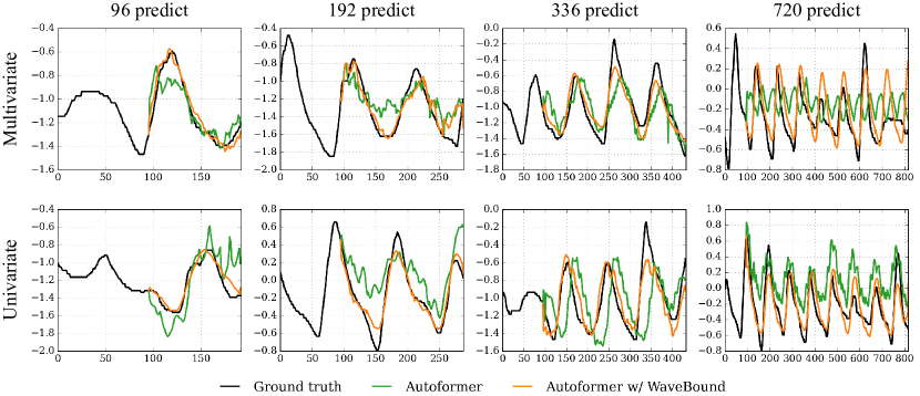
Figure 6: Qualitative results of Autoformer with and without WaveBound on the ETTm2 dataset. When using WaveBound, the results are relatively smoother and have less lag.

Quantitative Results. The additional experimental results of our proposed WaveBound method for full benchamrks and baselines are reported in Table 14, 15, and 16.

Qualitative Results. To illustrate the effects of WaveBound, we depict the predictions of different models on ETTm2 dataset (96 input). For the multivariate setting, we plot the predictions for the last feature. As shown in Figure 6, the models trained with WaveBound consistently predict accurately regardless of forecast step.

Appendix E Effects of $\epsilon$ in WaveBound

Table 4 shows the results for different hyperparameter values of $\epsilon$ which are searched in $\{0.01,0.001\}$. The performance can be improved by selecting proper $\epsilon$ in each setting.

Table 4: Performance comparison under difference choices of hyperparameter $\epsilon\in\{0.01,0.001\}$. We evaluate the performance of Autoformer on two different datasets ETT and Electricity.

		ETTm2				Electricity
		96	192	336	720	96	192	336	720
$\epsilon=0.01$	MSE	0.206	0.268	0.323	0.414	0.185	0.205	0.217	0.260
	MAE	0.290	0.327	0.361	0.412	0.300	0.317	0.327	0.359
$\epsilon=0.001$	MSE	0.204	0.265	0.320	0.413	0.176	0.233	0.228	0.282
	MAE	0.285	0.322	0.356	0.408	0.288	0.333	0.331	0.379

Appendix F Performance Analysis on Synthetic Dataset

Synthetic dataset. To analyze how WaveBound behaves in different noise levels and different dataset sizes, we synthesize a dataset composed of sine wave with the Gaussian noise. Formally, for a given noise level $\sigma$ and a time step $t$, the synthetic dataset is formed as: $f(t)=2\sin(2\pi t/32)+\sin(2\pi t/48)+\sigma z$, where $z$ follows the normal distribution.

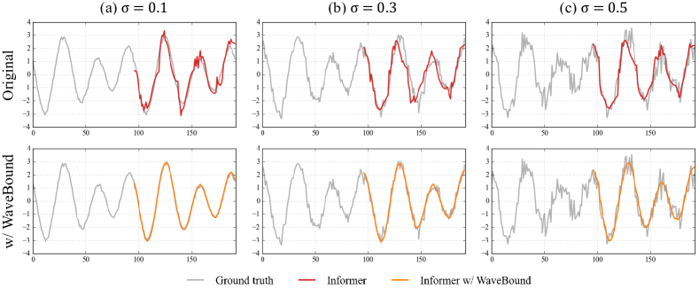
Figure 7: Qualitative results of Informer trained with and without WaveBound on the synthetic dataset. As the noise level $\sigma$ increases, Informer (top) is highly affected by the noise and produces the unstable predictions. In contrast, the model with WaveBound (bottom) shows the relatively stable predictions and correctly estimate the trend of the signal regardless of the noise level in the dataset.

Analysis on different noise levels and dataset sizes. In time series forecasting, the overfitting issue becomes significant when the train data is small and the data contains a high level of noise. Using the synthetic dataset, we examine the effectiveness of WaveBound in different levels of overfitting. Specifically, we examine Informer [7] trained with and without WaveBound by varying the noise level $\sigma$ and the datset size $|\mathcal{D}|$ of the synthetic dataset. Table 5 and Table 6 shows the performance of Informer with and without WaveBound in different noise levels and dataset sizes, respectively. As the noise level increases and dataset size decreases, Informer struggles with the unpredictable noise and produces noisy predictions, resulting in poor performance while WaveBound improves performance in all noise levels and dataset sizes. Figure 7 qualitatively shows that WaveBound allows the model to make stable predictions even in the high level of noise.

Table 5: Performance comparison under different noise levels $\sigma\in\{0.1,0.3,0.5\}$ with the fixed dataset size $|\mathcal{D}|=2000$. All results are averaged over 3 trials. Subscripts denote standard deviations.

		$\sigma=0.1$	$\sigma=0.3$	$\sigma=0.5$
Informer	MSE	0.225$\pm$0.024	0.316$\pm$0.022	0.605$\pm$0.061
	MAE	0.363$\pm$0.017	0.441$\pm$0.013	0.613$\pm$0.029
Informer w/ WaveBound	MSE	0.015$\pm$0.001	0.102$\pm$0.001	0.281$\pm$0.001
	MAE	0.096$\pm$0.003	0.252$\pm$0.002	0.419$\pm$0.000

Table 6: Performance comparison under different dataset sizes $|\mathcal{D}|\in\{4000,3000,2000\}$, with the fixed noise level $\sigma=0.5$. All results are averaged over 3 trials. Subscripts denote standard deviations.

		$|\mathcal{D}|=4000$	$|\mathcal{D}|=3000$	$|\mathcal{D}|=2000$
Informer	MSE	0.311$\pm$0.004	0.399$\pm$0.003	0.605$\pm$0.061
	MAE	0.443$\pm$0.003	0.505$\pm$0.002	0.613$\pm$0.029
Informer w/ WaveBound	MSE	0.246$\pm$0.001	0.290$\pm$0.002	0.281$\pm$0.001
	MAE	0.394$\pm$0.000	0.435$\pm$0.001	0.419$\pm$0.000

Appendix G Impact of WaveBound on Individual Features and Time Steps

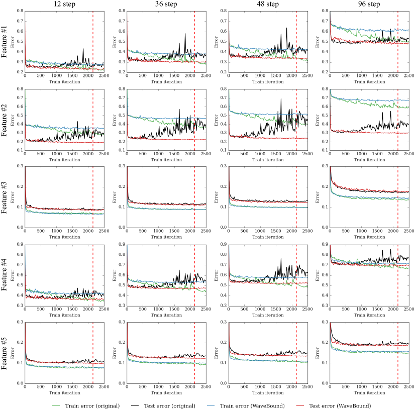
Figure 8: Training curve for each feature and time step of Autoformer on the ETTm2 dataset. Each row and column denote the feature and time step of the prediction, respectively. The red dotted line denotes the iteration of best checkpoint found by early-stopping. As we hypothesized, the output variables for different features and time steps show different trends for their training curves, which indicates that the consideration for each value is essential to properly handle the overfitting issue in time series forecasting.

To properly address an overfitting issue, WaveBound estimates adequate error bounds for each feature and time step individually. To justify the assumptions made by WaveBound, we depict the training curve of each feature and time step of the prediction made by Autoformer on the ETTm2 dataset. Each row and column in Figure 8 denote one feature and one time step, respectively. As we assumed, we can observe that different features show different training dynamics, which indicates that the difficulty of prediction varies through the features. Moreover, the magnitude of error increases as the forecast step increases. Those observations highlight that different regularization strategies are required for different features and time steps.

We also observe that existing regularization methods such as early-stopping cannot properly handle the overfitting issue, as it considers only the aggregated value rather than considering each error individually. Red dotted lines in Figure 8 denote the iteration of the best checkpoint found by early-stopping. Interestingly, even before the best checkpoint is decided by the early-stopping (red dotted lines), the model seems to be overfitted for several features; the train error (green line) is decreasing, but the test error (black line) is increasing. We conjecture that this is because of the property of the early-stopping, which considers only the mean value of error rather than individual errors of each feature and time step. In contrast, WaveBound retains the test loss (red lines) at a low level by preventing the train error (blue lines) from falling below a certain level for each feature and time step. In practice, this results in an overall performance improvement in time series forecasting, as shown in our extensive experiments.

Appendix H WaveBound with RevIN

Reversible instance normalization (RevIN) [41] is recently proposed to mitigate the distribution shift problem in time series forecasting. In this section, we conduct the additional experiments by applying both WaveBound and RevIN in training. As shown in Table 7, the performance of Autoformer [5] and Informer [7] is improved with a significant margin when both WaveBound and RevIN are applied.

Table 7: The results of WaveBound with RevIN. All results are averaged over 3 trials. Subscripts denote standard deviations.

Models Autoformer Informer Origin RevIN RevIN w/ WaveBound Origin RevIN RevIN w/ WaveBound Metric MSE MAE MSE MAE MSE MAE MSE MAE MSE MAE MSE MAE ETTm2 96 0.262 $\pm$0.037 0.326 $\pm$0.014 0.230 $\pm$0.007 0.303 $\pm$0.006 0.208 $\pm$0.002 0.282 $\pm$0.002 0.376 $\pm$0.056 0.477 $\pm$0.047 0.270 $\pm$0.041 0.326 $\pm$0.025 0.206 $\pm$0.000 0.286 $\pm$0.001 192 0.284 $\pm$0.003 0.342 $\pm$0.002 0.291 $\pm$0.005 0.338 $\pm$0.003 0.268 $\pm$0.001 0.319 $\pm$0.001 0.751 $\pm$0.020 0.672 $\pm$0.004 0.475 $\pm$0.078 0.439 $\pm$0.033 0.293 $\pm$0.011 0.341 $\pm$0.008 336 0.338 $\pm$0.007 0.374 $\pm$0.005 0.346 $\pm$0.004 0.369 $\pm$0.004 0.329 $\pm$0.000 0.357 $\pm$0.000 1.440 $\pm$0.180 0.917 $\pm$0.067 0.517 $\pm$0.089 0.467 $\pm$0.041 0.367 $\pm$0.005 0.385 $\pm$0.003 720 0.446 $\pm$0.011 0.435 $\pm$0.006 0.435 $\pm$0.010 0.419 $\pm$0.007 0.417 $\pm$0.003 0.407 $\pm$0.001 3.897 $\pm$0.562 1.498 $\pm$0.128 0.646 $\pm$0.075 0.531 $\pm$0.034 0.476 $\pm$0.015 0.442 $\pm$0.007 ECL 96 0.202 $\pm$0.003 0.317 $\pm$0.003 0.178 $\pm$0.001 0.285 $\pm$0.001 0.173 $\pm$0.008 0.276 $\pm$0.006 0.335 $\pm$0.008 0.417 $\pm$0.004 0.196 $\pm$0.001 0.303 $\pm$0.000 0.166 $\pm$0.001 0.269 $\pm$0.001 192 0.235 $\pm$0.011 0.340 $\pm$0.009 0.218 $\pm$0.010 0.317 $\pm$0.009 0.212 $\pm$0.017 0.308 $\pm$0.015 0.341 $\pm$0.013 0.426 $\pm$0.011 0.217 $\pm$0.004 0.322 $\pm$0.004 0.181 $\pm$0.003 0.283 $\pm$0.003 336 0.247 $\pm$0.011 0.351 $\pm$0.009 0.241 $\pm$0.016 0.335 $\pm$0.013 0.223 $\pm$0.019 0.318 $\pm$0.014 0.369 $\pm$0.011 0.448 $\pm$0.009 0.236 $\pm$0.004 0.339 $\pm$0.003 0.194 $\pm$0.002 0.297 $\pm$0.003 720 0.270 $\pm$0.006 0.371 $\pm$0.003 0.259 $\pm$0.006 0.349 $\pm$0.003 0.251 $\pm$0.021 0.342 $\pm$0.017 0.396 $\pm$0.009 0.457 $\pm$0.005 0.267 $\pm$0.001 0.363 $\pm$0.001 0.217 $\pm$0.001 0.317 $\pm$0.000

Appendix I WaveBound in Short-Term Series Forecasting

In this section, we examine WaveBound in short-term series forecasting. Specifically, we use Autoformer [5] as the baseline and train the model to forecast 3, 6, and 12 steps on ECL, exchange rate, and traffic dataset. Table 8 shows that WaveBound still achieves the performance improvements even in short-term series forecasting.

Table 8: Short-term forecasting results of WaveBound in the multivariate setting. We use ECL, exchange rate and traffic dataset with three prediction lengths $L\in\{3,6,12\}$. All results are averaged over 3 trials. Subscripts denote standard deviations.

Models		Autoformer
		Origin		w/ Ours
Metric		MSE	MAE	MSE	MAE
ECL	3	0.148$\pm$0.001	0.274$\pm$0.001	0.133$\pm$0.002	0.256$\pm$0.002
	6	0.152$\pm$0.001	0.277$\pm$0.000	0.140$\pm$0.001	0.263$\pm$0.001
	12	0.157$\pm$0.001	0.282$\pm$0.002	0.144$\pm$0.001	0.265$\pm$0.001
Exchange	3	0.034$\pm$0.003	0.132$\pm$0.005	0.029$\pm$0.009	0.121$\pm$0.020
	6	0.030$\pm$0.003	0.126$\pm$0.007	0.030$\pm$0.007	0.124$\pm$0.016
	12	0.039$\pm$0.004	0.143$\pm$0.007	0.032$\pm$0.005	0.129$\pm$0.008
Traffic	3	0.555$\pm$0.005	0.385$\pm$0.007	0.520$\pm$0.002	0.352$\pm$0.002
	6	0.555$\pm$0.001	0.377$\pm$0.003	0.531$\pm$0.001	0.351$\pm$0.003
	12	0.557$\pm$0.004	0.375$\pm$0.004	0.530$\pm$0.006	0.343$\pm$0.004

Appendix J WaveBound in Spatial-Temporal Time Series Forecasting

To examine the applicability of our WaveBound method in spatial-temporal time series forecasting, we examine Graph WaveNet [42] trained with and without WaveBound on a widely used traffic dataset, METR-LA [1]. As in Wu et al. [42], Graph WaveNet is trained with the mean absolute error and attempt to predict a future traffic speed of 1 hour given a historical data of 1 hour along with a graph structure. Table 9 shows that WaveBound improves the performance of Graph WaveNet in terms of all metrics, mean absolute error (MAE), root mean squared error (RMSE), and mean absolute precentage error (MAPE).

Table 9: Spatial-temporal forecasting results of WaveBound adopted to Graph WaveNet. All results are averaged over 3 trials.

Models	15min			30min			60min
	MAE	RMSE	MAPE	MAE	RMSE	MAPE	MAE	RMSE	MAPE
Graph WaveNet [42]	2.70	5.17	6.93%	3.10	6.24	8.37%	3.58	7.44	10.10%
+ WaveBound	2.67	5.11	6.91%	3.03	6.10	8.32%	3.45	7.15	9.90%

Appendix K Ablation Study on EMA Methods

Ablation study on the effect of EMA methods is shown in the Table 10. In the experiments, models only with EMA update (Without Bound) shows the slight performance improvements compared to the original model. However, EMA with dynamic error bound (WaveBound (Indiv.)) outperforms other baselines with a large margin, which concretely shows the effectiveness of individual error bounding in WaveBound.

Table 10: Results of EMA methods on the ECL dataset. All results are averaged over 3 trials. Subscripts denote standard deviations.

Models Origin Without Bound WaveBound (Avg.) WaveBound (Indiv.) Metric MSE MAE MSE MAE MSE MAE MSE MAE Autoformer 96 0.202$\pm$0.003 0.317$\pm$0.003 0.193$\pm$0.001 0.308$\pm$0.001 0.194$\pm$0.001 0.309$\pm$0.001 0.176$\pm$0.003 0.288$\pm$0.003 336 0.247$\pm$0.011 0.351$\pm$0.009 0.224$\pm$0.006 0.334$\pm$0.003 0.221$\pm$0.009 0.331$\pm$0.006 0.217$\pm$0.006 0.327$\pm$0.005 Pyraformer 96 0.256$\pm$0.002 0.360$\pm$0.001 0.247$\pm$0.002 0.351$\pm$0.002 0.248$\pm$0.002 0.352$\pm$0.002 0.241$\pm$0.001 0.345$\pm$0.001 336 0.278$\pm$0.007 0.383$\pm$0.006 0.287$\pm$0.009 0.388$\pm$0.010 0.288$\pm$0.011 0.388$\pm$0.010 0.269$\pm$0.005 0.371$\pm$0.005 Informer 96 0.335$\pm$0.008 0.417$\pm$0.004 0.305$\pm$0.005 0.391$\pm$0.006 0.302$\pm$0.004 0.388$\pm$0.003 0.289$\pm$0.003 0.378$\pm$0.002 336 0.369$\pm$0.011 0.448$\pm$0.009 0.326$\pm$0.017 0.411$\pm$0.013 0.322$\pm$0.010 0.407$\pm$0.008 0.305$\pm$0.008 0.394$\pm$0.008 LSTNet 96 0.268$\pm$0.004 0.366$\pm$0.003 0.201$\pm$0.002 0.311$\pm$0.003 0.208$\pm$0.010 0.314$\pm$0.010 0.185$\pm$0.003 0.291$\pm$0.003 336 0.284$\pm$0.001 0.382$\pm$0.002 0.241$\pm$0.004 0.352$\pm$0.004 0.246$\pm$0.009 0.356$\pm$0.009 0.217$\pm$0.004 0.326$\pm$0.005

Appendix L WaveBound with Small-Scale Model

We also evaluate the performance of WaveBound with the small-scale model. Specifically, we train a multi layer perceptron (MLP) model consisting of three linear layers with and without WaveBound in the univariate setting. Table 11 shows that WaveBound improves the performance of this MLP model.

Table 11: Results of the MLP model consisting of three linear layers with and without WaveBound in the univariate setting. All results are averaged over 3 trials. Subscripts denote standard deviations.

Models		Origin		w/ Ours
Metric		MSE	MAE	MSE	MAE
ETTm2	96	0.071$\pm$0.001	0.195$\pm$0.002	0.068$\pm$0.000	0.191$\pm$0.001
	192	0.105$\pm$0.004	0.243$\pm$0.005	0.104$\pm$0.000	0.241$\pm$0.001
	336	0.141$\pm$0.009	0.289$\pm$0.010	0.136$\pm$0.001	0.284$\pm$0.001
	720	0.207$\pm$0.010	0.357$\pm$0.009	0.194$\pm$0.002	0.343$\pm$0.002
ECL	96	0.325$\pm$0.003	0.401$\pm$0.001	0.317$\pm$0.003	0.392$\pm$0.002
	192	0.334$\pm$0.001	0.408$\pm$0.001	0.330$\pm$0.004	0.401$\pm$0.001
	336	0.389$\pm$0.007	0.446$\pm$0.007	0.380$\pm$0.002	0.436$\pm$0.001
	720	0.441$\pm$0.005	0.486$\pm$0.002	0.438$\pm$0.002	0.481$\pm$0.001

Appendix M WaveBound with Generative Model

To show the applicability of WaveBound when training a model with a loss function other than MSE we mainly considered in Section 3, we conduct an experiment with a generative model DeepAR [43] which uses a negative log likelihood (NLL) as a training objective. Table 12 shows that WaveBound improves the performance of DeepAR in the univariate setting.

Table 12: Results of DeepAR with and without WaveBound. All results are averaged over 3 trials. Subscripts denote standard deviations.

Models		DeepAR
		Origin		w/ Ours
Metric		NLL	MSE	MLL	MSE
ECL	8	1.059$\pm$0.152	0.447$\pm$0.168	0.935$\pm$0.045	0.306$\pm$0.001
	16	1.168$\pm$0.101	0.500$\pm$0.208	1.148$\pm$0.052	0.371$\pm$0.036
	24	1.256$\pm$0.073	0.617$\pm$0.119	1.180$\pm$0.062	0.394$\pm$0.043

Appendix N Computational Cost Analysis

WaveBound introduces additional computation and memory costs in the training phase as it employs the EMA model during training. In this section, we analyze the computation and memory cost of WaveBound on the ETTm2 dataset. The input and output lengths are fixed to 96 and a single TITAN RTX GPU is used for all experiments. Table 13 shows the computation time per epoch and maximum GPU memory occupied in the training phase. We also remark that WaveBound does not introduce the additional computation and memory costs in the inference phase.

Table 13: Computation cost analysis of WaveBound.

	Training time (Sec / Epoch)		GPU memory (GB)
Model	Origin	WaveBound	Origin	WaveBound
Autoformer	67.722	84.075	2.13	2.20
Pyraformer	27.024	39.083	0.47	0.50
Informer	75.251	97.154	1.80	1.86
LSTNet	20.380	23.347	0.02	0.02

Appendix O Limitations

While we observe the success of WaveBound with various baselines on real-world benchmarks, our method inevitably introduces the additional cost in the training procedure since our method utilizes the exponential moving average network for estimating the difficulty of predictions. Note that our method performs as the regularization technique in training and does not introduce any additional cost during inference.

Appendix P Potential Societal Impact

Our proposed method does not introduce any foreseeable societal consequence. The real-world benchmarks used in this work are widely used for research purposes.

Table 14: Results of WaveBound in the multivariate setting. All results are averaged over 3 trials. Subscripts denote standard deviations.

Models Autoformer [5] Pyraformer [6] Informer [7] LSTNet [14] TCN [16] Origin w/ Ours Origin w/ Ours Origin w/ Ours Origin w/ Ours Origin w/ Ours Metric MSE MAE MSE MAE MSE MAE MSE MAE MSE MAE MSE MAE MSE MAE MSE MAE MSE MAE MSE MAE ETTh1 96 0.443 $\pm$0.019 0.453 $\pm$0.012 0.395 $\pm$0.011 0.423 $\pm$0.007 0.637 $\pm$0.017 0.592 $\pm$0.007 0.630 $\pm$0.011 0.598 $\pm$0.013 0.886 $\pm$0.020 0.730 $\pm$0.014 0.841 $\pm$0.013 0.708 $\pm$0.010 0.662 $\pm$0.022 0.588 $\pm$0.009 0.660 $\pm$0.007 0.586 $\pm$0.002 0.704 $\pm$0.095 0.642 $\pm$0.056 0.692 $\pm$0.009 0.638 $\pm$0.005 192 0.509 $\pm$0.032 0.486 $\pm$0.020 0.433 $\pm$0.002 0.444 $\pm$0.001 0.814 $\pm$0.033 0.708 $\pm$0.020 0.807 $\pm$0.050 0.708 $\pm$0.034 0.988 $\pm$0.014 0.781 $\pm$0.009 0.959 $\pm$0.015 0.755 $\pm$0.010 0.771 $\pm$0.008 0.652 $\pm$0.008 0.716 $\pm$0.004 0.617 $\pm$0.001 0.831 $\pm$0.027 0.722 $\pm$0.019 0.830 $\pm$0.003 0.711 $\pm$0.002 336 0.519 $\pm$0.024 0.502 $\pm$0.017 0.470 $\pm$0.005 0.476 $\pm$0.004 0.903 $\pm$0.024 0.749 $\pm$0.014 0.859 $\pm$0.026 0.728 $\pm$0.016 1.159 $\pm$0.073 0.861 $\pm$0.027 1.097 $\pm$0.040 0.826 $\pm$0.019 0.882 $\pm$0.004 0.712 $\pm$0.002 0.782 $\pm$0.004 0.664 $\pm$0.007 0.894 $\pm$0.016 0.739 $\pm$0.007 0.935 $\pm$0.004 0.758 $\pm$0.003 720 0.516 $\pm$0.013 0.517 $\pm$0.009 0.503 $\pm$0.017 0.506 $\pm$0.010 0.932 $\pm$0.007 0.767 $\pm$0.004 0.919 $\pm$0.011 0.763 $\pm$0.006 1.178 $\pm$0.020 0.861 $\pm$0.006 1.164 $\pm$0.002 0.867 $\pm$0.003 1.030 $\pm$0.034 0.804 $\pm$0.013 0.856 $\pm$0.017 0.721 $\pm$0.010 1.139 $\pm$0.030 0.824 $\pm$0.013 1.067 $\pm$0.012 0.793 $\pm$0.004 ETTh2 96 0.392 $\pm$0.033 0.417 $\pm$0.016 0.338 $\pm$0.002 0.379 $\pm$0.002 1.453 $\pm$0.254 0.938 $\pm$0.083 1.269 $\pm$0.015 0.912 $\pm$0.007 2.967 $\pm$0.296 1.349 $\pm$0.068 2.261 $\pm$0.357 1.178 $\pm$0.098 1.189 $\pm$0.017 0.876 $\pm$0.018 1.011 $\pm$0.107 0.767 $\pm$0.057 3.038 $\pm$0.217 1.399 $\pm$0.059 2.921 $\pm$0.203 1.370 $\pm$0.040 192 0.467 $\pm$0.023 0.459 $\pm$0.013 0.420 $\pm$0.005 0.428 $\pm$0.003 5.147 $\pm$0.708 1.822 $\pm$0.137 2.072 $\pm$0.075 1.172 $\pm$0.029 5.822 $\pm$0.644 1.999 $\pm$0.121 5.361 $\pm$0.646 1.929 $\pm$0.115 2.227 $\pm$0.436 1.193 $\pm$0.160 1.612 $\pm$0.075 0.991 $\pm$0.014 6.275 $\pm$0.909 2.096 $\pm$0.170 5.060 $\pm$0.762 1.865 $\pm$0.171 336 0.472 $\pm$0.004 0.475 $\pm$0.003 0.452 $\pm$0.003 0.459 $\pm$0.002 4.381 $\pm$0.188 1.736 $\pm$0.048 2.299 $\pm$0.094 1.273 $\pm$0.041 4.926 $\pm$0.260 1.864 $\pm$0.051 4.700 $\pm$0.181 1.878 $\pm$0.046 2.274 $\pm$0.111 1.235 $\pm$0.030 1.697 $\pm$0.207 1.041 $\pm$0.094 6.887 $\pm$0.936 2.245 $\pm$0.149 4.263 $\pm$0.291 1.747 $\pm$0.073 720 0.485 $\pm$0.010 0.496 $\pm$0.009 0.454 $\pm$0.009 0.468 $\pm$0.003 4.304 $\pm$0.530 1.764 $\pm$0.110 2.810 $\pm$0.098 1.458 $\pm$0.033 3.885 $\pm$0.351 1.667 $\pm$0.089 3.791 $\pm$0.168 1.642 $\pm$0.057 2.447 $\pm$0.079 1.286 $\pm$0.020 1.861 $\pm$0.062 1.114 $\pm$0.027 8.993 $\pm$2.254 2.355 $\pm$0.321 3.299 $\pm$0.073 1.504 $\pm$0.010 ETTm1 96 0.491 $\pm$0.028 0.467 $\pm$0.013 0.385 $\pm$0.002 0.416 $\pm$0.003 0.480 $\pm$0.015 0.490 $\pm$0.010 0.495 $\pm$0.017 0.494 $\pm$0.009 0.654 $\pm$0.044 0.576 $\pm$0.016 0.590 $\pm$0.008 0.543 $\pm$0.002 0.607 $\pm$0.010 0.541 $\pm$0.009 0.508 $\pm$0.021 0.484 $\pm$0.009 0.603 $\pm$0.031 0.558 $\pm$0.013 0.556 $\pm$0.008 0.531 $\pm$0.006 192 0.571 $\pm$0.013 0.504 $\pm$0.008 0.500 $\pm$0.002 0.472 $\pm$0.001 0.572 $\pm$0.021 0.544 $\pm$0.021 0.525 $\pm$0.013 0.523 $\pm$0.008 0.783 $\pm$0.050 0.658 $\pm$0.023 0.672 $\pm$0.012 0.595 $\pm$0.011 0.615 $\pm$0.019 0.559 $\pm$0.007 0.563 $\pm$0.007 0.525 $\pm$0.002 0.702 $\pm$0.014 0.610 $\pm$0.002 0.632 $\pm$0.009 0.577 $\pm$0.006 336 0.611 $\pm$0.029 0.526 $\pm$0.008 0.497 $\pm$0.047 0.475 $\pm$0.015 0.750 $\pm$0.081 0.650 $\pm$0.031 0.629 $\pm$0.023 0.592 $\pm$0.012 1.097 $\pm$0.046 0.810 $\pm$0.024 0.889 $\pm$0.016 0.724 $\pm$0.009 0.657 $\pm$0.009 0.593 $\pm$0.006 0.652 $\pm$0.053 0.581 $\pm$0.015 0.881 $\pm$0.034 0.705 $\pm$0.012 0.749 $\pm$0.005 0.643 $\pm$0.005 720 0.605 $\pm$0.031 0.527 $\pm$0.010 0.507 $\pm$0.044 0.488 $\pm$0.017 0.949 $\pm$0.022 0.749 $\pm$0.005 0.806 $\pm$0.052 0.691 $\pm$0.028 1.277 $\pm$0.036 0.855 $\pm$0.010 1.095 $\pm$0.022 0.797 $\pm$0.004 0.785 $\pm$0.050 0.667 $\pm$0.022 0.720 $\pm$0.013 0.628 $\pm$0.015 1.047 $\pm$0.023 0.767 $\pm$0.010 0.910 $\pm$0.008 0.714 $\pm$0.003 ETTm2 96 0.262 $\pm$0.037 0.326 $\pm$0.014 0.204 $\pm$0.001 0.285 $\pm$0.001 0.363 $\pm$0.089 0.451 $\pm$0.064 0.281 $\pm$0.026 0.386 $\pm$0.021 0.376 $\pm$0.056 0.477 $\pm$0.047 0.334 $\pm$0.025 0.429 $\pm$0.026 0.455 $\pm$0.096 0.511 $\pm$0.067 0.268 $\pm$0.006 0.368 $\pm$0.006 0.537 $\pm$0.128 0.555 $\pm$0.080 0.480 $\pm$0.039 0.524 $\pm$0.020 192 0.284 $\pm$0.003 0.342 $\pm$0.002 0.265 $\pm$0.002 0.322 $\pm$0.002 0.708 $\pm$0.044 0.648 $\pm$0.023 0.624 $\pm$0.011 0.599 $\pm$0.006 0.751 $\pm$0.020 0.672 $\pm$0.004 0.698 $\pm$0.056 0.631 $\pm$0.013 0.706 $\pm$0.102 0.660 $\pm$0.064 0.464 $\pm$0.027 0.508 $\pm$0.020 0.928 $\pm$0.110 0.745 $\pm$0.054 0.812 $\pm$0.030 0.708 $\pm$0.013 336 0.338 $\pm$0.007 0.374 $\pm$0.005 0.320 $\pm$0.001 0.356 $\pm$0.001 1.130 $\pm$0.086 0.846 $\pm$0.026 1.072 $\pm$0.016 0.829 $\pm$0.008 1.440 $\pm$0.180 0.917 $\pm$0.067 1.087 $\pm$0.064 0.845 $\pm$0.026 1.161 $\pm$0.066 0.868 $\pm$0.049 0.781 $\pm$0.012 0.695 $\pm$0.009 1.118 $\pm$0.097 0.816 $\pm$0.037 1.015 $\pm$0.104 0.775 $\pm$0.057 720 0.446 $\pm$0.011 0.435 $\pm$0.006 0.413 $\pm$0.001 0.408 $\pm$0.000 2.995 $\pm$0.095 1.386 $\pm$0.046 1.917 $\pm$0.074 1.119 $\pm$0.028 3.897 $\pm$0.562 1.498 $\pm$0.128 2.984 $\pm$0.127 1.411 $\pm$0.042 3.288 $\pm$0.102 1.494 $\pm$0.048 2.312 $\pm$0.358 1.239 $\pm$0.105 2.687 $\pm$0.302 1.231 $\pm$0.078 2.120 $\pm$0.042 1.092 $\pm$0.011

Table 15: Results of WaveBound in the multivariate setting. All results are averaged over 3 trials. Subscripts denote standard deviations.

Models Autoformer [5] Pyraformer [6] Informer [7] LSTNet [14] TCN [16] Origin w/ Ours Origin w/ Ours Origin w/ Ours Origin w/ Ours Origin w/ Ours Metric MSE MAE MSE MAE MSE MAE MSE MAE MSE MAE MSE MAE MSE MAE MSE MAE MSE MAE MSE MAE Electricity 96 0.202 $\pm$0.003 0.317 $\pm$0.003 0.176 $\pm$0.003 0.288 $\pm$0.003 0.256 $\pm$0.002 0.360 $\pm$0.001 0.241 $\pm$0.001 0.345 $\pm$0.001 0.335 $\pm$0.008 0.417 $\pm$0.004 0.289 $\pm$0.003 0.378 $\pm$0.002 0.268 $\pm$0.004 0.366 $\pm$0.003 0.185 $\pm$0.003 0.291 $\pm$0.003 0.268 $\pm$0.003 0.363 $\pm$0.003 0.260 $\pm$0.002 0.353 $\pm$0.002 192 0.235 $\pm$0.011 0.340 $\pm$0.009 0.205 $\pm$0.003 0.317 $\pm$0.004 0.272 $\pm$0.003 0.378 $\pm$0.003 0.256 $\pm$0.002 0.360 $\pm$0.002 0.341 $\pm$0.013 0.426 $\pm$0.011 0.298 $\pm$0.002 0.388 $\pm$0.002 0.277 $\pm$0.002 0.375 $\pm$0.001 0.197 $\pm$0.003 0.304 $\pm$0.003 0.295 $\pm$0.006 0.385 $\pm$0.005 0.272 $\pm$0.003 0.358 $\pm$0.002 336 0.247 $\pm$0.011 0.351 $\pm$0.009 0.217 $\pm$0.006 0.327 $\pm$0.005 0.278 $\pm$0.007 0.383 $\pm$0.006 0.269 $\pm$0.005 0.371 $\pm$0.005 0.369 $\pm$0.011 0.448 $\pm$0.009 0.305 $\pm$0.008 0.394 $\pm$0.008 0.284 $\pm$0.001 0.382 $\pm$0.002 0.217 $\pm$0.004 0.326 $\pm$0.005 0.309 $\pm$0.013 0.394 $\pm$0.009 0.284 $\pm$0.003 0.365 $\pm$0.002 720 0.270 $\pm$0.006 0.371 $\pm$0.003 0.260 $\pm$0.024 0.359 $\pm$0.018 0.291 $\pm$0.002 0.385 $\pm$0.001 0.283 $\pm$0.003 0.377 $\pm$0.003 0.396 $\pm$0.009 0.457 $\pm$0.005 0.311 $\pm$0.008 0.398 $\pm$0.008 0.316 $\pm$0.002 0.404 $\pm$0.001 0.250 $\pm$0.001 0.350 $\pm$0.002 0.310 $\pm$0.002 0.388 $\pm$0.002 0.290 $\pm$0.003 0.369 $\pm$0.001 Exchange 96 0.153 $\pm$0.009 0.285 $\pm$0.009 0.146 $\pm$0.005 0.274 $\pm$0.007 0.604 $\pm$0.037 0.624 $\pm$0.016 0.615 $\pm$0.037 0.627 $\pm$0.015 0.979 $\pm$0.045 0.791 $\pm$0.021 0.878 $\pm$0.053 0.765 $\pm$0.032 0.483 $\pm$0.030 0.518 $\pm$0.017 0.357 $\pm$0.046 0.432 $\pm$0.028 0.805 $\pm$0.116 0.707 $\pm$0.060 0.720 $\pm$0.023 0.693 $\pm$0.014 192 0.297 $\pm$0.030 0.397 $\pm$0.019 0.262 $\pm$0.001 0.373 $\pm$0.001 0.982 $\pm$0.093 0.806 $\pm$0.029 0.953 $\pm$0.076 0.797 $\pm$0.031 1.147 $\pm$0.110 0.854 $\pm$0.042 1.136 $\pm$0.021 0.859 $\pm$0.014 0.706 $\pm$0.042 0.646 $\pm$0.027 0.621 $\pm$0.210 0.593 $\pm$0.111 0.945 $\pm$0.079 0.795 $\pm$0.042 0.912 $\pm$0.035 0.781 $\pm$0.020 336 0.438 $\pm$0.018 0.490 $\pm$0.011 0.425 $\pm$0.001 0.483 $\pm$0.001 1.264 $\pm$0.131 0.934 $\pm$0.052 1.263 $\pm$0.043 0.944 $\pm$0.014 1.592 $\pm$0.067 1.014 $\pm$0.016 1.461 $\pm$0.051 0.992 $\pm$0.014 1.055 $\pm$0.124 0.800 $\pm$0.049 0.837 $\pm$0.055 0.691 $\pm$0.027 1.350 $\pm$0.105 0.962 $\pm$0.035 1.135 $\pm$0.045 0.889 $\pm$0.023 720 1.207 $\pm$0.080 0.860 $\pm$0.034 1.088 $\pm$0.004 0.810 $\pm$0.002 1.663 $\pm$0.083 1.051 $\pm$0.019 1.562 $\pm$0.097 1.016 $\pm$0.012 2.540 $\pm$0.089 1.306 $\pm$0.027 2.496 $\pm$0.253 1.294 $\pm$0.071 2.198 $\pm$0.656 1.127 $\pm$0.189 1.374 $\pm$0.139 0.894 $\pm$0.040 2.061 $\pm$0.226 1.152 $\pm$0.076 1.689 $\pm$0.162 1.067 $\pm$0.045 Traffic 96 0.645 $\pm$0.011 0.399 $\pm$0.012 0.596 $\pm$0.027 0.352 $\pm$0.013 0.635 $\pm$0.006 0.364 $\pm$0.006 0.622 $\pm$0.003 0.341 $\pm$0.003 0.731 $\pm$0.010 0.412 $\pm$0.001 0.671 $\pm$0.007 0.364 $\pm$0.004 0.735 $\pm$0.008 0.446 $\pm$0.003 0.587 $\pm$0.004 0.356 $\pm$0.003 0.645 $\pm$0.007 0.361 $\pm$0.005 0.633 $\pm$0.004 0.333 $\pm$0.003 192 0.644 $\pm$0.027 0.407 $\pm$0.021 0.607 $\pm$0.013 0.370 $\pm$0.014 0.658 $\pm$0.006 0.376 $\pm$0.005 0.646 $\pm$0.001 0.355 $\pm$0.000 0.751 $\pm$0.007 0.422 $\pm$0.007 0.666 $\pm$0.005 0.360 $\pm$0.005 0.750 $\pm$0.001 0.446 $\pm$0.000 0.595 $\pm$0.005 0.365 $\pm$0.004 0.646 $\pm$0.001 0.354 $\pm$0.001 0.625 $\pm$0.002 0.320 $\pm$0.001 336 0.625 $\pm$0.021 0.390 $\pm$0.019 0.603 $\pm$0.019 0.361 $\pm$0.017 0.668 $\pm$0.003 0.377 $\pm$0.001 0.653 $\pm$0.002 0.355 $\pm$0.002 0.822 $\pm$0.003 0.465 $\pm$0.003 0.709 $\pm$0.014 0.387 $\pm$0.009 0.778 $\pm$0.002 0.455 $\pm$0.000 0.623 $\pm$0.019 0.378 $\pm$0.014 0.661 $\pm$0.005 0.363 $\pm$0.003 0.630 $\pm$0.001 0.320 $\pm$0.001 720 0.650 $\pm$0.008 0.398 $\pm$0.004 0.642 $\pm$0.011 0.383 $\pm$0.007 0.698 $\pm$0.002 0.390 $\pm$0.001 0.672 $\pm$0.001 0.364 $\pm$0.002 0.957 $\pm$0.038 0.539 $\pm$0.024 0.764 $\pm$0.025 0.421 $\pm$0.014 0.815 $\pm$0.002 0.470 $\pm$0.002 0.648 $\pm$0.008 0.383 $\pm$0.009 0.655 $\pm$0.001 0.358 $\pm$0.001 0.634 $\pm$0.000 0.322 $\pm$0.000 Weather 96 0.294 $\pm$0.014 0.355 $\pm$0.011 0.227 $\pm$0.008 0.296 $\pm$0.010 0.235 $\pm$0.010 0.321 $\pm$0.010 0.193 $\pm$0.007 0.272 $\pm$0.005 0.378 $\pm$0.029 0.428 $\pm$0.016 0.355 $\pm$0.014 0.415 $\pm$0.009 0.237 $\pm$0.004 0.310 $\pm$0.002 0.202 $\pm$0.007 0.275 $\pm$0.004 0.447 $\pm$0.008 0.481 $\pm$0.008 0.412 $\pm$0.013 0.457 $\pm$0.010 192 0.308 $\pm$0.004 0.368 $\pm$0.005 0.283 $\pm$0.005 0.340 $\pm$0.005 0.340 $\pm$0.041 0.415 $\pm$0.032 0.306 $\pm$0.015 0.372 $\pm$0.006 0.462 $\pm$0.012 0.467 $\pm$0.002 0.424 $\pm$0.003 0.448 $\pm$0.007 0.277 $\pm$0.003 0.343 $\pm$0.003 0.254 $\pm$0.000 0.316 $\pm$0.002 0.604 $\pm$0.023 0.558 $\pm$0.012 0.618 $\pm$0.006 0.558 $\pm$0.008 336 0.364 $\pm$0.007 0.396 $\pm$0.008 0.335 $\pm$0.013 0.370 $\pm$0.010 0.453 $\pm$0.038 0.484 $\pm$0.028 0.403 $\pm$0.055 0.441 $\pm$0.037 0.575 $\pm$0.010 0.535 $\pm$0.005 0.506 $\pm$0.017 0.484 $\pm$0.009 0.326 $\pm$0.007 0.378 $\pm$0.004 0.309 $\pm$0.015 0.358 $\pm$0.012 0.753 $\pm$0.017 0.632 $\pm$0.007 0.689 $\pm$0.049 0.587 $\pm$0.024 720 0.426 $\pm$0.014 0.433 $\pm$0.013 0.401 $\pm$0.001 0.411 $\pm$0.002 0.599 $\pm$0.045 0.563 $\pm$0.025 0.535 $\pm$0.011 0.519 $\pm$0.007 1.024 $\pm$0.067 0.751 $\pm$0.025 0.972 $\pm$0.065 0.712 $\pm$0.030 0.412 $\pm$0.007 0.431 $\pm$0.007 0.398 $\pm$0.006 0.415 $\pm$0.004 0.947 $\pm$0.050 0.722 $\pm$0.019 0.876 $\pm$0.075 0.661 $\pm$0.033 ILI 24 3.468 $\pm$0.252 1.299 $\pm$0.058 3.118 $\pm$0.036 1.200 $\pm$0.019 4.822 $\pm$0.081 1.489 $\pm$0.015 4.679 $\pm$0.087 1.459 $\pm$0.024 5.356 $\pm$0.062 1.590 $\pm$0.016 4.947 $\pm$0.053 1.494 $\pm$0.017 7.934 $\pm$0.304 2.091 $\pm$0.031 6.331 $\pm$0.231 1.816 $\pm$0.029 4.561 $\pm$0.065 1.535 $\pm$0.015 4.093 $\pm$0.060 1.378 $\pm$0.030 36 3.441 $\pm$0.139 1.273 $\pm$0.034 3.310 $\pm$0.192 1.240 $\pm$0.049 4.831 $\pm$0.196 1.479 $\pm$0.041 4.763 $\pm$0.198 1.483 $\pm$0.044 5.131 $\pm$0.046 1.569 $\pm$0.006 5.027 $\pm$0.081 1.537 $\pm$0.022 8.793 $\pm$0.428 2.214 $\pm$0.047 6.560 $\pm$0.629 1.848 $\pm$0.088 4.376 $\pm$0.249 1.463 $\pm$0.077 4.213 $\pm$0.361 1.425 $\pm$0.107 48 3.086 $\pm$0.176 1.184 $\pm$0.036 2.927 $\pm$0.017 1.128 $\pm$0.010 4.789 $\pm$0.153 1.465 $\pm$0.036 4.524 $\pm$0.132 1.439 $\pm$0.029 5.150 $\pm$0.037 1.564 $\pm$0.010 4.920 $\pm$0.047 1.514 $\pm$0.009 7.968 $\pm$0.255 2.068 $\pm$0.026 6.154 $\pm$0.110 1.779 $\pm$0.019 4.264 $\pm$0.085 1.418 $\pm$0.022 3.963 $\pm$0.221 1.340 $\pm$0.062 60 2.843 $\pm$0.025 1.136 $\pm$0.010 2.785 $\pm$0.021 1.116 $\pm$0.003 4.876 $\pm$0.027 1.495 $\pm$0.006 4.573 $\pm$0.158 1.465 $\pm$0.026 5.407 $\pm$0.033 1.604 $\pm$0.011 5.013 $\pm$0.059 1.528 $\pm$0.016 7.387 $\pm$0.269 1.984 $\pm$0.036 6.119 $\pm$0.186 1.758 $\pm$0.031 4.288 $\pm$0.105 1.401 $\pm$0.033 3.970 $\pm$0.108 1.335 $\pm$0.032

Table 16: Results of WaveBound in the univariate setting. All results are averaged over 3 trials. Subscripts denote standard deviations.

Models Autoformer [5] Pyraformer [6] Informer [7] N-BEATS [15] LSTNet [14] TCN [16] Origin w/ Ours Origin w/ Ours Origin w/ Ours Origin w/ Ours Origin w/ Ours Origin w/ Ours Metric MSE MAE MSE MAE MSE MAE MSE MAE MSE MAE MSE MAE MSE MAE MSE MAE MSE MAE MSE MAE MSE MAE MSE MAE ETTm2 96 0.098 $\pm$0.016 0.239 $\pm$0.020 0.085 $\pm$0.004 0.221 $\pm$0.005 0.078 $\pm$0.007 0.209 $\pm$0.011 0.070 $\pm$0.002 0.197 $\pm$0.003 0.085 $\pm$0.008 0.224 $\pm$0.012 0.081 $\pm$0.003 0.218 $\pm$0.004 0.073 $\pm$0.004 0.198 $\pm$0.006 0.067 $\pm$0.001 0.188 $\pm$0.002 0.091 $\pm$0.008 0.228 $\pm$0.011 0.067 $\pm$0.001 0.188 $\pm$0.001 0.082 $\pm$0.011 0.218 $\pm$0.017 0.073 $\pm$0.001 0.207 $\pm$0.001 192 0.130 $\pm$0.012 0.277 $\pm$0.012 0.116 $\pm$0.008 0.262 $\pm$0.008 0.114 $\pm$0.003 0.257 $\pm$0.004 0.110 $\pm$0.004 0.256 $\pm$0.004 0.122 $\pm$0.007 0.273 $\pm$0.009 0.118 $\pm$0.001 0.270 $\pm$0.002 0.107 $\pm$0.007 0.246 $\pm$0.010 0.103 $\pm$0.001 0.241 $\pm$0.001 0.125 $\pm$0.005 0.272 $\pm$0.006 0.108 $\pm$0.001 0.248 $\pm$0.002 0.142 $\pm$0.016 0.295 $\pm$0.015 0.113 $\pm$0.002 0.265 $\pm$0.003 336 0.162 $\pm$0.005 0.311 $\pm$0.003 0.143 $\pm$0.008 0.293 $\pm$0.008 0.178 $\pm$0.007 0.325 $\pm$0.003 0.153 $\pm$0.006 0.306 $\pm$0.005 0.153 $\pm$0.004 0.304 $\pm$0.003 0.148 $\pm$0.001 0.305 $\pm$0.002 0.163 $\pm$0.028 0.310 $\pm$0.027 0.135 $\pm$0.001 0.284 $\pm$0.001 0.171 $\pm$0.002 0.322 $\pm$0.002 0.159 $\pm$0.004 0.308 $\pm$0.004 0.157 $\pm$0.022 0.314 $\pm$0.026 0.154 $\pm$0.002 0.314 $\pm$0.003 720 0.194 $\pm$0.001 0.344 $\pm$0.002 0.188 $\pm$0.004 0.338 $\pm$0.002 0.198 $\pm$0.024 0.351 $\pm$0.016 0.169 $\pm$0.005 0.329 $\pm$0.005 0.196 $\pm$0.005 0.351 $\pm$0.006 0.189 $\pm$0.003 0.349 $\pm$0.003 0.263 $\pm$0.033 0.402 $\pm$0.026 0.188 $\pm$0.006 0.340 $\pm$0.006 0.253 $\pm$0.003 0.395 $\pm$0.003 0.242 $\pm$0.003 0.387 $\pm$0.002 0.248 $\pm$0.038 0.404 $\pm$0.034 0.193 $\pm$0.002 0.360 $\pm$0.001 Electricity 96 0.462 $\pm$0.023 0.502 $\pm$0.014 0.447 $\pm$0.029 0.496 $\pm$0.022 0.240 $\pm$0.002 0.351 $\pm$0.001 0.229 $\pm$0.002 0.347 $\pm$0.002 0.266 $\pm$0.005 0.371 $\pm$0.003 0.261 $\pm$0.006 0.369 $\pm$0.005 0.304 $\pm$0.001 0.382 $\pm$0.001 0.298 $\pm$0.005 0.378 $\pm$0.002 0.452 $\pm$0.011 0.505 $\pm$0.006 0.340 $\pm$0.022 0.419 $\pm$0.013 0.235 $\pm$0.003 0.357 $\pm$0.001 0.226 $\pm$0.005 0.346 $\pm$0.004 192 0.557 $\pm$0.016 0.565 $\pm$0.013 0.515 $\pm$0.031 0.538 $\pm$0.017 0.262 $\pm$0.005 0.367 $\pm$0.001 0.253 $\pm$0.001 0.365 $\pm$0.001 0.283 $\pm$0.003 0.385 $\pm$0.003 0.281 $\pm$0.006 0.383 $\pm$0.003 0.323 $\pm$0.002 0.396 $\pm$0.001 0.322 $\pm$0.004 0.395 $\pm$0.002 0.419 $\pm$0.007 0.477 $\pm$0.003 0.327 $\pm$0.005 0.402 $\pm$0.001 0.284 $\pm$0.008 0.389 $\pm$0.007 0.272 $\pm$0.004 0.382 $\pm$0.003 336 0.613 $\pm$0.026 0.593 $\pm$0.015 0.531 $\pm$0.044 0.543 $\pm$0.028 0.285 $\pm$0.002 0.386 $\pm$0.002 0.283 $\pm$0.002 0.386 $\pm$0.002 0.338 $\pm$0.005 0.428 $\pm$0.003 0.332 $\pm$0.005 0.426 $\pm$0.004 0.385 $\pm$0.004 0.430 $\pm$0.001 0.369 $\pm$0.001 0.422 $\pm$0.000 0.439 $\pm$0.011 0.488 $\pm$0.006 0.352 $\pm$0.003 0.420 $\pm$0.001 0.378 $\pm$0.015 0.451 $\pm$0.009 0.327 $\pm$0.012 0.419 $\pm$0.007 720 0.691 $\pm$0.045 0.632 $\pm$0.019 0.604 $\pm$0.009 0.591 $\pm$0.004 0.309 $\pm$0.002 0.411 $\pm$0.002 0.307 $\pm$0.016 0.415 $\pm$0.016 0.631 $\pm$0.008 0.612 $\pm$0.004 0.378 $\pm$0.005 0.463 $\pm$0.004 0.462 $\pm$0.009 0.487 $\pm$0.004 0.433 $\pm$0.003 0.473 $\pm$0.001 0.492 $\pm$0.004 0.528 $\pm$0.003 0.428 $\pm$0.032 0.478 $\pm$0.016 0.435 $\pm$0.044 0.490 $\pm$0.026 0.399 $\pm$0.060 0.471 $\pm$0.035

References

- [1] Yaguang Li, Rose Yu, Cyrus Shahabi, and Yan Liu. Diffusion convolutional recurrent neural network: Data-driven traffic forecasting. In Proc. the International Conference on Learning Representations (ICLR), 2018.
- [2] Yue Pang, Bo Yao, Xiangdong Zhou, Yong Zhang, Yiming Xu, and Zijing Tan. Hierarchical electricity time series forecasting for integrating consumption patterns analysis and aggregation consistency. In Proc. the International Joint Conference on Artificial Intelligence (IJCAI), 2018.
- [3] Xiao Ding, Yue Zhang, Ting Liu, and Junwen Duan. Deep learning for event-driven stock prediction. In Proc. the International Joint Conference on Artificial Intelligence (IJCAI), 2015.
- [4] Yasuko Matsubara, Yasushi Sakurai, Willem G. van Panhuis, and Christos Faloutsos. FUNNEL: automatic mining of spatially coevolving epidemics. In Proc. the ACM SIGKDD International Conference on Knowledge Discovery and Data Mining (KDD), 2014.
- [5] Haixu Wu, Jiehui Xu, Jianmin Wang, and Mingsheng Long. Autoformer: Decomposition transformers with auto-correlation for long-term series forecasting. In Proc. the Advances in Neural Information Processing Systems (NeurIPS).
- [6] Shizhan Liu, Hang Yu, Cong Liao, Jianguo Li, Weiyao Lin, Alex X. Liu, and Schahram Dustdar. Pyraformer: Low-complexity pyramidal attention for long-range time series modeling and forecasting. In Proc. the International Conference on Learning Representations (ICLR), 2022.
- [7] Haoyi Zhou, Shanghang Zhang, Jieqi Peng, Shuai Zhang, Jianxin Li, Hui Xiong, and Wancai Zhang. Informer: Beyond efficient transformer for long sequence time-series forecasting. In Proc. the AAAI Conference on Artificial Intelligence (AAAI), 2021.
- [8] Shiyang Li, Xiaoyong Jin, Yao Xuan, Xiyou Zhou, Wenhu Chen, Yu-Xiang Wang, and Xifeng Yan. Enhancing the locality and breaking the memory bottleneck of transformer on time series forecasting. In Proc. the Advances in Neural Information Processing Systems (NeurIPS), 2019.
- [9] Nikita Kitaev, Lukasz Kaiser, and Anselm Levskaya. Reformer: The efficient transformer. In Proc. the International Conference on Learning Representations (ICLR), 2020.
- [10] Takashi Ishida, Ikko Yamane, Tomoya Sakai, Gang Niu, and Masashi Sugiyama. Do we need zero training loss after achieving zero training error? In Proc. the International Conference on Machine Learning (ICML), 2020.
- [11] Jean-Bastien Grill, Florian Strub, Florent Altché, Corentin Tallec, Pierre H. Richemond, Elena Buchatskaya, Carl Doersch, Bernardo Ávila Pires, Zhaohan Guo, Mohammad Gheshlaghi Azar, Bilal Piot, Koray Kavukcuoglu, Rémi Munos, and Michal Valko. Bootstrap your own latent - A new approach to self-supervised learning. In Proc. the Advances in Neural Information Processing Systems (NeurIPS), 2020.
- [12] Kaiming He, Haoqi Fan, Yuxin Wu, Saining Xie, and Ross B. Girshick. Momentum contrast for unsupervised visual representation learning. In Proc. of the IEEE conference on computer vision and pattern recognition (CVPR), 2020.
- [13] Antti Tarvainen and Harri Valpola. Mean teachers are better role models: Weight-averaged consistency targets improve semi-supervised deep learning results. In Proc. the Advances in Neural Information Processing Systems (NeurIPS), 2017.
- [14] Guokun Lai, Wei-Cheng Chang, Yiming Yang, and Hanxiao Liu. Modeling long- and short-term temporal patterns with deep neural networks. In SIGIR, 2018.
- [15] Boris N. Oreshkin, Dmitri Carpov, Nicolas Chapados, and Yoshua Bengio. N-BEATS: neural basis expansion analysis for interpretable time series forecasting. In Proc. the International Conference on Learning Representations (ICLR), 2020.
- [16] Shaojie Bai, J. Zico Kolter, and Vladlen Koltun. An empirical evaluation of generic convolutional and recurrent networks for sequence modeling. CoRR, abs/1803.01271, 2018.
- [17] Hao Li, Zheng Xu, Gavin Taylor, Christoph Studer, and Tom Goldstein. Visualizing the loss landscape of neural nets. In Proc. the Advances in Neural Information Processing Systems (NeurIPS), 2018.
- [18] Namuk Park and Songkuk Kim. How do vision transformers work? In Proc. the International Conference on Learning Representations (ICLR), 2022.
- [19] Xiangning Chen, Cho-Jui Hsieh, and Boqing Gong. When vision transformers outperform resnets without pretraining or strong data augmentations. In Proc. the International Conference on Learning Representations (ICLR), 2022.
- [20] George EP Box, Gwilym M Jenkins, and John F MacGregor. Some recent advances in forecasting and control. Journal of the Royal Statistical Society: Series C (Applied Statistics), 1974.
- [21] Sean J Taylor and Benjamin Letham. Forecasting at scale. The American Statistician, 72(1):37–45, 2018.
- [22] James Durbin and Siem Jan Koopman. Time series analysis by state space methods, volume 38. OUP Oxford, 2012.
- [23] Rob Hyndman, Anne B Koehler, J Keith Ord, and Ralph D Snyder. Forecasting with exponential smoothing: the state space approach. Springer Science & Business Media, 2008.
- [24] Yao Qin, Dongjin Song, Haifeng Chen, Wei Cheng, Guofei Jiang, and Garrison W. Cottrell. A dual-stage attention-based recurrent neural network for time series prediction. In Carles Sierra, editor, Proc. the International Joint Conference on Artificial Intelligence (IJCAI), 2017.
- [25] Ruofeng Wen, Kari Torkkola, Balakrishnan Narayanaswamy, and Dhruv Madeka. A multi-horizon quantile recurrent forecaster. arXiv preprint arXiv:1711.11053, 2017.
- [26] Huan Song, Deepta Rajan, Jayaraman J. Thiagarajan, and Andreas Spanias. Attend and diagnose: Clinical time series analysis using attention models. In Proc. the AAAI Conference on Artificial Intelligence (AAAI), 2018.
- [27] Daniel Stoller, Mi Tian, Sebastian Ewert, and Simon Dixon. Seq-u-net: A one-dimensional causal u-net for efficient sequence modelling. In Proc. the International Joint Conference on Artificial Intelligence (IJCAI), 2020.
- [28] Aäron van den Oord, Sander Dieleman, Heiga Zen, Karen Simonyan, Oriol Vinyals, Alex Graves, Nal Kalchbrenner, Andrew W. Senior, and Koray Kavukcuoglu. Wavenet: A generative model for raw audio. ISCA, 2016.
- [29] Rajat Sen, Hsiang-Fu Yu, and Inderjit S. Dhillon. Think globally, act locally: A deep neural network approach to high-dimensional time series forecasting. In Proc. the Advances in Neural Information Processing Systems (NeurIPS), 2019.
- [30] Syama Sundar Rangapuram, Matthias W. Seeger, Jan Gasthaus, Lorenzo Stella, Yuyang Wang, and Tim Januschowski. Deep state space models for time series forecasting. In Proc. the Advances in Neural Information Processing Systems (NeurIPS), 2018.
- [31] Emmanuel de Bézenac, Syama Sundar Rangapuram, Konstantinos Benidis, Michael Bohlke-Schneider, Richard Kurle, Lorenzo Stella, Hilaf Hasson, Patrick Gallinari, and Tim Januschowski. Normalizing kalman filters for multivariate time series analysis. In Proc. the Advances in Neural Information Processing Systems (NeurIPS), 2020.
- [32] Alexej Klushyn, Richard Kurle, Maximilian Soelch, Botond Cseke, and Patrick van der Smagt. Latent matters: Learning deep state-space models. In Proc. the Advances in Neural Information Processing Systems (NeurIPS), 2021.
- [33] Rahul G. Krishnan, Uri Shalit, and David A. Sontag. Structured inference networks for nonlinear state space models. In Proc. the AAAI Conference on Artificial Intelligence (AAAI), 2017.
- [34] Richard Kurle, Syama Sundar Rangapuram, Emmanuel de Bézenac, Stephan Günnemann, and Jan Gasthaus. Deep rao-blackwellised particle filters for time series forecasting. In Proc. the Advances in Neural Information Processing Systems (NeurIPS), 2020.
- [35] Abdul Fatir Ansari, Konstantinos Benidis, Richard Kurle, Ali Caner Türkmen, Harold Soh, Alexander J. Smola, Bernie Wang, and Tim Januschowski. Deep explicit duration switching models for time series. In Proc. the Advances in Neural Information Processing Systems (NeurIPS), 2021.
- [36] Stephen Jose Hanson and Lorien Y. Pratt. Comparing biases for minimal network construction with back-propagation. In Proc. the Advances in Neural Information Processing Systems (NeurIPS), 1988.
- [37] Nelson Morgan and Hervé Bourlard. Generalization and parameter estimation in feedforward netws: Some experiments. In Proc. the Advances in Neural Information Processing Systems (NeurIPS), 1989.
- [38] Nitish Srivastava, Geoffrey E. Hinton, Alex Krizhevsky, Ilya Sutskever, and Ruslan Salakhutdinov. Dropout: a simple way to prevent neural networks from overfitting. Journal of Machine Learning Research, 15:1929–1958, 2014.
- [39] Mahdy Shirdel, Reza Asadi, Duc Do, and Michael Hintlian. Deep learning with kernel flow regularization for time series forecasting. CoRR, abs/2109.11649, 2021.
- [40] Souhaib Ben Taieb, Jiafan Yu, Mateus Neves Barreto, and Ram Rajagopal. Regularization in hierarchical time series forecasting with application to electricity smart meter data. In Proc. the AAAI Conference on Artificial Intelligence (AAAI), 2017.
- [41] Taesung Kim, Jinhee Kim, Yunwon Tae, Cheonbok Park, Jang-Ho Choi, and Jaegul Choo. Reversible instance normalization for accurate time-series forecasting against distribution shift. In Proc. the International Conference on Learning Representations (ICLR), 2021.
- [42] Zonghan Wu, Shirui Pan, Guodong Long, Jing Jiang, and Chengqi Zhang. Graph wavenet for deep spatial-temporal graph modeling. In Sarit Kraus, editor, Proc. the International Joint Conference on Artificial Intelligence (IJCAI), 2019.
- [43] Valentin Flunkert, David Salinas, and Jan Gasthaus. Deepar: Probabilistic forecasting with autoregressive recurrent networks. CoRR, abs/1704.04110, 2017.