A novel approach to correcting $T_{e}$-based mass-metallicity relations

Abstract

Deriving oxygen abundances from the electron temperature (hereafter the $T_{e}$-method) is the gold-standard for extragalactic metallicity studies. However, unresolved temperature fluctuations within individual H ii regions and across different H ii regions throughout a galaxy can bias metallicity estimates low, with a magnitude that depends on the underlying and typically unknown temperature distribution. Using a toy model, we confirm that computing $T_{e}$-based metallicities using the temperature derived from the [O iii] $\lambda$4363/$\lambda$5007 or [O ii] $\lambda\lambda$7320,7330 / [O ii] $\lambda\lambda$3727 ratio (‘ratio temperature’; $T_{\rm ratio}$) results in an underprediction of metallicity when temperature fluctuations are present. In contrast, using the unobservable ‘line temperatures’ ($T_{\rm line}$) that provide the mean electron and ion density-weighted emissivity yield an accurate metallicity estimate. To correct this bias in low-mass galaxies, we demonstrate an example calibration of a relation between $T_{\rm ratio}$ and $T_{\rm line}$ based on a high-resolution (4.5 pc) RAMSES-RTZ simulation of a dwarf galaxy that self-consistently models the formation of multiple H ii regions and ion temperature distribution in a galactic context. Applying this correction to the low-mass end of the mass-metallicity relation shifts its normalization up by 0.18 dex on average and flattens its slope from 0.87 to 0.58, highlighting the need for future studies to account for, and correct, this bias.

1 Introduction

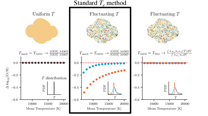
Figure 1: Toy-model demonstrating how temperature fluctuations bias the $T_{e}$-method when applied to a uniform metallicity system. From left to right, lower panels show the discrepancy between the true metallicity and that derived from Equation 1 for: a homogeneous cloud with uniform temperature and using $T_{\rm ratio}$ (the $T_{e}$ inferred from [O iii] $\lambda$4363/$\lambda$5007), a cloud with temperature fluctuations and using $T_{\rm ratio}$, and a cloud with temperature fluctuations and using $T_{\rm line}$ (Equation 2). Temperature fluctuations are either normally (blue) or lognormally (orange) distributed (insets). The standard $T_{e}$-method (centre panel) always underpredicts metallicity when temperature fluctuations are present, with the deficit depending on the exact shape of the temperature distribution. In contrast, when the cloud is homogeneous or when $T_{\rm line}$ is used, the metallicity prediction is accurate.

The gas-phase oxygen abundance (‘metallicity’ hereafter) of a galaxy is a fundamental property that encodes a wealth of information on its star formation, enrichment, and assembly history. Galaxy metallicity exhibits a tight correlation with stellar mass, the mass-metallicity relation (MZR; e.g. Lequeux et al. 1979, Tremonti et al. 2004), with scatter in this relation correlating with star formation rate (e.g. Ellison et al., 2008; Mannucci et al., 2010) and gas mass (e.g. Bothwell et al., 2013). Measurements of the slope and normalisation of this relation are interpreted as the collective effect of metal-enriched outflows and metal-poor inflows (e.g. Larson, 1974; Dalcanton et al., 2004; Tremonti et al., 2004), and used to constrain astrophysical models that predict the chemical enrichment and assembly histories of galaxies (e.g. Ma et al., 2016; De Rossi et al., 2017; Torrey et al., 2019).

However, the exact shape of the MZR remains debated, as its slope and normalisation is sensitive to the technique used to measure metallicity (e.g. Kewley & Ellison, 2008; Curti et al., 2020; Yates et al., 2020). Using recombination lines (RL) is often considered the most robust metallicity estimate, due to its weak dependence on gas temperature and density. But it relies on measuring multiple faint metal lines, which is possible in the local neighbourhood of the Milky Way (e.g. Peimbert et al., 1993; Esteban et al., 2002) but prohibitive for extragalactic samples. In contrast, strong-line methods rely only on ratios of the brightest emission lines and can therefore be widely applied. However, they need to be calibrated to more direct measurements (e.g. Curti et al., 2017) or theoretical predictions (e.g. McGaugh, 1991; Kewley et al., 2019), each associated with dificult-to-quantify systematic uncertainties (Kewley & Ellison, 2008).

As a result, the $T_{e}$ method (Peimbert, 1967) has been the de facto gold standard for measurements of the MZR (e.g. Andrews & Martini 2013, hereafter AM13; Curti et al. 2020). It relies on detecting auroral emission lines (e.g. [O iii] $\lambda$4363) to estimate $T_{e}$, enabling us to derive metallicities solely from line emissivities based on collision strengths from quantum mechanical calculations (e.g. Aggarwal & Keenan, 1999; Palay et al., 2012; Storey et al., 2014). Detecting such faint auroral lines is observationally challenging, but possible at low-redshift for large samples of individual low-metallicity galaxies (e.g. Izotov et al., 2019) or stacks of higher-metallicity galaxies (Curti et al., 2017). Further, the advent of JWST now allows us to make such detections at high-redshift (e.g. at $z=8.5$; Katz et al. 2022a; Curti et al. 2022). The central role played by the $T_{e}$-method to constrain chemical evolution across cosmic time makes it paramount to pinpoint its potential biases and losses of accuracy.

In fact, $T_{e}$-method metallicities are typically lower than RL techniques by as much as $\sim 0.3$ dex in observations where both can be computed (e.g. Liu et al., 2001; García-Rojas & Esteban, 2007). A promising explanation for these offsets is the presence of inhomogeneous temperatures for the emission-line emitting gas, which then biases the $T_{e}$-method metallicity measurements low due to the exponential scaling of line emissivities with temperature (Peimbert 1967; Stasińska 2005; Bresolin 2008; Pilyugin et al. 2012; Section 2). Such temperature inhomogeneities can originate within individual H ii regions due to their internal structure (see Peimbert 2019 for a review), but also across a galaxy, as the multiple H ii regions integrated into a galactic spectrum are subject to a diversity of ISM densities, temperatures and feedback conditions. Although $T_{e}$-metallicities can be debiased by measuring multiple temperatures for the same system to estimate the underlying distribution (Peimbert & Costero 1969; Peimbert et al. 2004), such observations are typically restricted to nearby, individual H ii regions and are rarely feasible for distant galaxies.

Pinpointing the importance of galactic-scale temperature fluctuations is thus essential to calibrate the true magnitude of this long-standing bias and recover accurate extragalactic $T_{e}$-metallicities. In this paper, we introduce a new physically-motivated model to achieve this aim. Rather than estimating temperature fluctuations from measurements of local H ii regions (e.g. Kobulnicky et al., 1999) or photoionization models (Stasińska, 1990; Garnett, 1992), we use a high-resolution ($\approx 4.5$ pc) simulation of an isolated dwarf galaxy with multifrequency radiation-hydrodynamics coupled to non-equilibrium metal and molecular chemistry. This allows us to self-consistently predict the distribution of H ii region temperatures, across an entire galaxy undergoing star formation and feedback episodes. We estimate the resulting bias in $T_{e}$ metallicities (Section 3) and how it affects the derived MZR (Section 4).

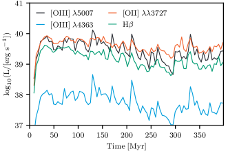
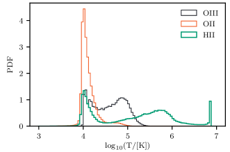
Figure 2: (Top) Evolution of the emission line luminosities needed to apply the [O III] $T_{e}$ method as a function of time in the simulation. (Bottom) Example ion mass-weighted temperature distribution derived from the simulation at 400 Myr, showcasing the extended and non-trivial temperature distribution at a particular time.

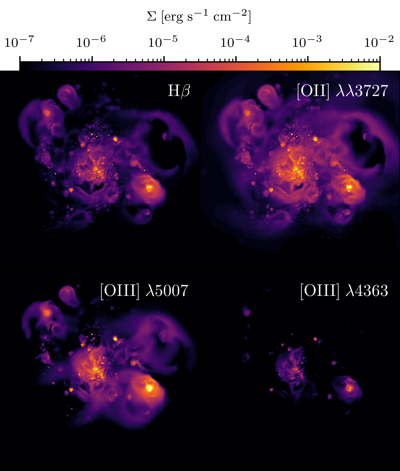
Figure 3: 4.5 kpc maps of H$\beta$, [O ii] $\lambda\lambda$3727, [O iii] $\lambda$5007, and [O iii] $\lambda$4363, surface brightness at $t=400$ Myr, showing the spatial variations across H ii regions at a given time.

2 How temperature fluctuations affect $T_{e}$-based metallicities

To gain insights into the importance of sub-resolution temperature fluctuations, we construct a toy model that derives $T_{e}$-metallicities from O ii and O iii emission lines which are generally readily available for extragalactic studies. Ionized oxygen and hydrogen trace each other in the ISM due to their near-identical ionization potentials and a strong coupling from charge exchange reactions. Assuming in these ionized regions that the O⁺ and O⁺⁺ ionization states dominate, the metallicity is:

$$\frac{\rm O}{\rm H}\approx\frac{{\rm O}^{+}}{{\rm H}^{+}}+\frac{{\rm O}^{++}}{{\rm H}^{+}}=\frac{L_{\lambda\lambda 3727}}{L_{\rm H\beta}}\frac{\epsilon_{\rm H\beta}(T_{1})}{\epsilon_{\lambda\lambda 3727}(T_{2})}+\frac{L_{\lambda 5007}}{L_{\rm H\beta}}\frac{\epsilon_{\rm H\beta}(T_{3})}{\epsilon_{\lambda 5007}(T_{4})},$$ (1)

where $L_{\lambda 5007}$, $L_{\lambda\lambda 3727}$, and $L_{\rm H\beta}$ are the observed luminosities of the [O iii] $\lambda 5007$, [O ii] $\lambda\lambda 3727$, and H$\beta$ lines, and $\epsilon_{\lambda 5007}$, $\epsilon_{\lambda\lambda 3727}$, and $\epsilon_{\rm H\beta}$ are their emissivities.

The key to this calculation is the measurement of the temperature. It is typical to assume $T_{3}=T_{4}$ and adopt the ratio temperature ($T_{\rm ratio}$) measured from the [O iii] $\lambda 4363$/[O iii] $\lambda 5007$ ratio. Then $T_{1}=T_{2}$ are either measured from [O ii] auroral lines, or derived by assuming a relation between the O ii and O iii temperatures (e.g. Pérez-Montero, 2017). Indeed, applying Equation 1 with $T_{\rm ratio}$ to a single parcel of gas with uniform temperature provides an unbiased estimate of the metallicity, which depends only on atomic physics (Figure 1, left).

However, when multiple parcels of gas with a range of temperatures are present, we can introduce the ‘line temperature’, $T_{\rm line}$ (e.g. Stasińska, 1978):

$$\epsilon_{\lambda}(T_{\rm line})=\frac{\int n_{X_{i}}n_{e}\epsilon_{\lambda}(T)dV}{\int n_{X_{i}}n_{e}dV},$$ (2)

where $n_{e}$ is the electron density, $n_{X_{i}}$ is the number density of species $X_{i}$ with a transition that gives rise to an emission line with wavelength $\lambda$, and $\epsilon_{\lambda}$ is the emissivity of that line. $T_{\rm line}$ encodes the average emissivity of each emission line across the range of probed temperatures, weighted by the local electron and ion densities. This quantity is related to the intrinsic ‘ionic temperature’ (the mass-weighted average temperature of a given ion), however $T_{\rm line}$ is more directly related to observed emission line fluxes as it additionally encodes information of how emissivity scales with temperature. The crux of the bias described in Section 1 is that, since the emissivity of H$\beta$, [O ii] $\lambda\lambda 3727$, and [O iii] $\lambda 5007$ scale differently with temperature, each line has a different $T_{\rm line}$ differing from $T_{\rm ratio}$. Hence using $T_{\rm ratio}$ in Equation 1 can result in an incorrect metallicity.

To gauge the magnitude of this effect, we construct a system comprised of 1,000 gas parcels, all with constant metallicity of $12+\log_{10}({\rm O/H})=8.48$, randomized electron densities between $10^{-1}-10^{3}\ {\rm cm^{-3}}$, and randomized temperatures. We construct 28 systems assuming either a normal ($\sigma=10^{3}$ K) or lognormal ($\sigma=0.3$ dex) temperature distribution, each with 14 different mean temperature values ranging from 7,000 K to 20,000 K. Within each parcel, the gas temperature is the same for each ion. We then obtain the total luminosities of [O iii] $\lambda 5007$, [O iii] $\lambda 4363$, [O ii] $\lambda\lambda 3727$, and H$\beta$ by summing the emergent luminosities from each gas parcel. Applying the $T_{e}$-method, we compute the ‘measured’ metallicity of the system by deriving $T_{\rm ratio}$ from [O iii] $\lambda 4363$/$\lambda 5007$ and inputting this into Equation 1. The centre panel of Figure 1 shows that metallicities derived using $T_{\rm ratio}$ systematically underpredict the true value, and the magnitude of the bias strongly depends on both the shape of the temperature distribution (blue versus orange) and its mean temperature (left to right). Since mean temperature is often correlated with galaxy metallicity, temperature fluctuations can affect relative metallicity measurements, and impact the shape of the MZR.

In contrast, if we adopt the corresponding $T_{\rm line}$ for each $T_{i}$ in Equation 1, we obtain an unbiased metallicity measurement, regardless of the underlying temperature distribution (Figure 1 right panel). However, $T_{\rm line}$ is not a directly measurable quantity. Given that the sub-resolution temperature distributions in real galaxies are much more complicated than the simple distributions presented here, this motivates a theoretical approach to predicting what distribution the temperatures in a realistic galaxy might take. Thus, we now present a new, physically-motivated exploration of the temperature distribution in a simulated isolated dwarf galaxy. Based on this, we outline a novel method to convert $T_{\rm ratio}$ to $T_{\rm line}$ and debias $T_{e}$-derived metallicities.

3 Quantifying temperature fluctuations in a simulated dwarf galaxy

We now make use of novel numerical methods that allow us to directly predict the temperature distribution of H ii regions within a simulated galaxy, and estimate a relation between $T_{\rm ratio}$ and $T_{\rm line}$.

3.1 Simulation methods

Our simulations achieve a resolution of 4.5 pc across the ISM, resolving the structure of large H ii regions. Using the out-of-equilibrium temperatures, ionization states, and electron densities self-consistently produced by the simulation, we solve for equilibrium level populations to predict emission line luminosities. We follow Katz et al. (2022c) to compute Balmer lines according to the most recent atomic data in CHIANTI (Dere et al., 2019), while oxygen line luminosities are calculated with PyNEB (Luridiana et al., 2015). We simulate the same isolated dwarf galaxy as in Katz (2022) with a halo mass of $10^{10}\ {\rm M_{\odot}}$, a circular velocity of $30\ {\rm km\ s^{-1}}$, a disk gas mass of $3.5\times 10^{8}\ {\rm M_{\odot}}$, and an initial central metallicity of $10^{-1}Z_{\odot}$ (see Katz 2022, Section 4 for further details). We then evolve these initial conditions using the RAMSES-RTZ code (Katz, 2022) and the PRISM interstellar medium (ISM) model for cooling and heating (Katz et al., 2022b). We improve the resolution by a factor 4 compared to Katz (2022) to better resolve H ii regions, and run the simulation for twice as long.

Radiation hydrodynamics is self-consistently computed in eight energy bins (Kimm et al. 2017, Table 2), assuming a reduced speed of light ($c_{\rm sim}=c/100$), and is coupled to the non-equilibrium chemistry of eight ionization states of O, seven of N, six of C, and six of Si, Mg, Fe, S, and Ne, and all ionization states of H and He. We account for star formation, stellar feedback and enrichment from massive stars (Katz 2022, Section 4), and apply a Haardt & Madau (2012) UV background which is exponentially suppressed at $\rho>10^{-2}\ {\rm cm^{-3}}$. We employ a fixed cosmic-ray background ionization rate of $\eta_{\rm cr}=10^{-16}\ {\rm s^{-1}H^{-1}}$. We highlight that ISM conditions are sensitive to the choice of feedback model (e.g. Roca-Fàbrega et al., 2021), and that future works are required to assess the extent of these uncertainties and how they affect the robustness of derived temperature fluctuations in simulated galaxies. Similarly, uncertainties associated with numerical metal mixing could affect the distribution of metals and their temperature distributions. In particular, adaptive mesh refinement (AMR), as used in this study, can over-mix the fluid (e.g. Wadsley et al., 2008) and smooth out metal (and temperature) distributions. This would, however, decrease temperature fluctuations across the galaxy, making results in this section conservative with respect to this issue.

3.2 Abundance discrepancy in our simulated galaxy

To provide the cleanest test of the $T_{e}$-method, we work only with the intrinsic luminosities so as to not introduce uncertainties due to dust attenuation. We assume that we detect [O ii] $\lambda\lambda$3727, [O ii] $\lambda\lambda$7320, 7330, [O iii] $\lambda$5007, [O iii] $\lambda$4363, and H$\beta$. While it is rare to simultaneously detect the [O ii] and [O iii] auroral lines in the same galaxy, this provides the cleanest test of the accuracy of the direct method.

We evolve the galaxy for 400 Myr. After the initial starburst relaxes from the initial conditions, the star formation rate (SFR) fluctuates in the range $10^{-2}<{\rm SFR/M_{\odot}yr^{-1}}<10^{-1}$. These temporal fluctuations are reflected on the galaxy-integrated emission line luminosities needed for the $T_{e}$-method (Figure 2, top panel). We further show in the bottom panel of Figure 2 the ion mass-weighted temperature distributions for O iii, O ii, and H ii at the end of the simulation, and emission-line maps (Figure 3). At a given time, the dynamic ISM environment generates an extended ion temperature distribution with non-trivial shape, and an irregular emission line spatial distribution. These temperature fluctuations will cause a bias in the $T_{e}$-method.

From the simulated [O ii] $\lambda\lambda$3727, [O ii] $\lambda\lambda$7320, 7330, [O iii] $\lambda$5007, [O iii] $\lambda$4363, and H$\beta$ luminosities, we then calculate metallicity using the standard direct method (Equation 1) using the ratio temperature derived from [O iii] $\lambda 4363$ / [O iii] $\lambda 5007$ for O iii and [O ii] $\lambda\lambda$7320,7330 / [O ii] $\lambda\lambda$3727 for O ii. We further compute the unobservable $T_{\rm line}$ (Equation 2) for [O ii] $\lambda\lambda$3727, [O iii] $\lambda$5007 and H$\beta$ using the self-consistent simulated distribution of temperatures, electron and ion densities, and compare the derived metallicities between the two in Figure 4. Using $T_{\rm ratio}$ results in a systematic underprediction with an average deficit of 0.21 dex, ranging between at $0.1-0.5$ dex during the course of the simulation (colours). These offsets have comparable magnitude to discrepancies between $T_{e}$ and RL metallicities (García-Rojas & Esteban, 2007), and between galaxy-integrated measurements compared to combining their individual H ii regions (Kobulnicky et al., 1999).

A possible avenue to correct such abundance discrepancy is to use the $t^{2}$-method (Peimbert & Costero, 1969), in which ion temperatures are measured from multiple different tracers to better estimate their underlying temperature distribution. However, detecting multiple independent temperature tracers is highly challenging beyond the local Universe, limiting the applicability of this approach for extragalactic studies. Instead, in the next section we introduce a novel approach in which we suggest that $T_{\rm ratio}$ can be converted to $T_{\rm line}$ which, as discussed in Section 2, results in an unbiased metallicity measurement. We foresee that this approach will be more widely applicable to extragalactic studies where most observations have at most one temperature tracer.

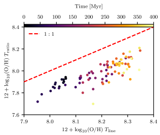
Figure 4: Metallicity measured with $T_{\rm line}$ vs. metallicity measured with $T_{\rm ratio}$ as a function of time. As the simulation progresses (colours), the metallicity of the galaxy grows but the $T_{\rm ratio}$-derived metallicity always results in a systematically lower value.

3.3 Calibrating the $T_{\rm line}$-$T_{\rm ratio}$ relation

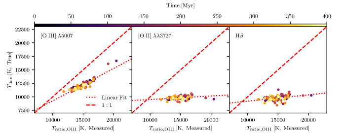
Figure 5: $T_{\rm ratio}$ from [O iii] $\lambda$4363/[O iii] $\lambda$5007 compared to the [O iii] $\lambda$5007 (left), [O ii] $\lambda\lambda$3727 (centre), and H$\beta$ (right) line temperatures. All $T_{\rm line}$ are systematically underpredicted by $T_{\rm ratio}$, but they exhibit a tight correlation for each emission line.

Figure 5 shows the ratio temperature as measured from [O iii] $\lambda$4363/$\lambda$5007 versus the line temperatures of [O iii] $\lambda$5007, [O ii] $\lambda\lambda$3727, and H$\beta$ for each time snapshot of our simulated galaxy between 50 and 400 Myr. The temperatures of all three lines are tightly correlated with $T_{\rm ratio}$, such that

$$\begin{split}T_{\rm line,\,[OIII]\,\lambda 5007}&=0.60\,T_{\rm ratio}+3258\ {\rm K},\\ T_{\rm line,\,[OII]\,\lambda\lambda 3727}&=0.065\,T_{\rm ratio}+8859\ {\rm K},\ \text{and}\\ T_{\rm line,\,H\beta}&=0.117\,T_{\rm ratio}+8034\ {\rm K}.\end{split}$$ (3)

We emphasise that these relations are derived from a single simulation of an isolated dwarf galaxy. It remains unclear how these generalise to galaxies of different masses, metallicities, and star formation rates, and how sensitive they are to the choice of feedback model. A detailed quantification on how to generalise the coefficients in Equation 3 across the whole galaxy population is beyond the scope of this work, and we stress that our determinations should not be applied blindly to large datasets. However, our simulation currently provides the most realistic estimate of temperature fluctuations across dwarf galaxies – we thus extrapolate them to a range of stellar masses in the next section to illustrate how accounting for temperature fluctuations could reshape the low-mass end of the MZR, strongly motivating future studies extending our analysis.

We note that the relations described in Equation 3 could also be derived in terms of $T_{\rm ratio}$(O ii). Indeed, at higher masses and metallicities, the [O ii] auroral lines may become the most accessible temperature diagnostic (e.g. Sanders et al., 2022). However, given that the [O iii] $\lambda$4363 / $\lambda$5007 ratio is the most widely used temperature diagnostic in extragalactic studies (especially in the dwarf galaxy regime), we have chosen to base the relations in Equation 3 on $T_{\rm ratio}$(O iii). Consideration of an O ii based $T_{\rm line}-T_{\rm ratio}$ relation is deferred to future work that will study higher mass and more metal-enriched galaxies.

4 Discussion and Conclusions

We have shown how temperature fluctuations within an H ii region and throughout a galaxy can bias $T_{e}$-method metallicities low, with a magnitude that depends on the shape and mean of the underlying distribution. While the existence of this bias is well established (e.g. Peimbert, 1967; Stasińska, 2005), estimating its magnitude and correcting it in extragalactic samples is challenging (e.g. Peimbert 1967, AM13). We propose a new solution based on deriving a relation between the observable $T_{\rm ratio}$ (that can be derived from auroral-to-nebular line ratios) to the unobservable $T_{\rm line}$, which we demonstrate provides a much more accurate temperature estimator for the $T_{e}$ method (Figure 1).

We calibrate this relation using high-resolution (4.5 pc) numerical simulations of a dwarf galaxy with RAMSES-RTZ that couple non-equilibrium metal chemistry to multi-frequency radiation hydrodynamics to estimate the temperature distributions across the warm-ionised gas in the galaxy. Applying the standard $T_{e}$-method to simulated data underpredicts the representative metallicity of H ii regions at all times, by 0.21 dex on average and up to 0.5 dex (Figure 4). Nonetheless, each line temperature tightly correlates with $T_{\rm ratio}$ from [O iii] (Figure 5), offering us the opportunity to debias metallicity estimates.

To illustrate the importance of accounting for unresolved temperature fluctuations when determining the MZR, we use the stacked SDSS spectra from AM13 for stellar mass bins below $10^{8.5}\ {\rm M_{\odot}}$, and apply the $T_{e}$-method from the [O iii] $\lambda$4363, [O iii] $\lambda$5007, [O ii] $\lambda\lambda$3727, and H$\beta$ fluxes. Figure 6 shows the resulting metallicities (black points), with the best fit (black line) using the functional form in AM13 (their Equation 5). The original fit to the MZR from AM13 (red line) shows minor differences due to their different atomic data, a different relation to convert between $T_{e}$ (O iii) and $T_{e}$(O ii), and their more extended stellar mass range for the fit.

Figure 6: MZR for SDSS galaxies based on the standard $T_{e}$ method using $T_{\rm ratio}$ (black), our updated $T_{e}$ method using the estimated $T_{\rm line}$ (blue), and the fit from AM13 (red). The slope of the MZR flattens and the normalization increases using our new approach to debiasing the measurement.

We then use Equation 3 to estimate $T_{\rm line}$ for each emission line before deriving the metallicity from Equation 1 and recalculate the MZR (blue points). The metallicity increases at all stellar masses, with the stellar-mass dependent offset reaching $\sim 0.3$ dex for lower mass bins, and flattens the measured slope of the MZR from 0.87 to 0.58.

Further work is needed to establish the robustness of applying Equation 3 derived from a single dwarf galaxy to the general sample from AM13 (as well as to other, potentially less biased, samples), however this experiment emphasizes that a careful quantification and correction of biases in metallicity measurements is essential to robustly interpret the MZR. We advocate for larger suites of comparable simulations than used in this study, across a larger range of stellar masses and metallicities, and in a cosmological context. Refining the relations presented in Equation 3 from such a suite of simulations could aid interpretations of observations in a manner comparable to how 1D photoionisation models (from e.g. CLOUDY or MAPPINGS) have historically been used.

Finally, other metallicity diagnostics that are readily-available for extragalactic samples, in particular theory-calibrated strong-line methods, have shown offsets compared to metallicities derived using $T_{e}$-based methods (e.g. AM13). We plan in future work to use similar simulations as used in this work to explore the physical nature of these offsets and propose new corrections to improve the robustness of metallicity estimates.

Data Availability

Underlying data will be shared on reasonable request to the authors.

References

- Aggarwal & Keenan (1999) Aggarwal K. M., Keenan F. P., 1999, ApJS, 123, 311
- Andrews & Martini (2013) Andrews B. H., Martini P., 2013, ApJ, 765, 140
- Bothwell et al. (2013) Bothwell M. S., Maiolino R., Kennicutt R., Cresci G., Mannucci F., Marconi A., Cicone C., 2013, MNRAS, 433, 1425
- Bresolin (2008) Bresolin F., 2008, in Israelian G., Meynet G., eds, The Metal-Rich Universe. p. 155 (arXiv:astro-ph/0608410)
- Curti et al. (2017) Curti M., Cresci G., Mannucci F., Marconi A., Maiolino R., Esposito S., 2017, MNRAS, 465, 1384
- Curti et al. (2020) Curti M., Mannucci F., Cresci G., Maiolino R., 2020, MNRAS, 491, 944
- Curti et al. (2022) Curti M., et al., 2022, MNRAS,
- Dalcanton et al. (2004) Dalcanton J. J., Yoachim P., Bernstein R. A., 2004, ApJ, 608, 189
- De Rossi et al. (2017) De Rossi M. E., Bower R. G., Font A. S., Schaye J., Theuns T., 2017, MNRAS, 472, 3354
- Dere et al. (2019) Dere K. P., Del Zanna G., Young P. R., Landi E., Sutherland R. S., 2019, ApJS, 241, 22
- Ellison et al. (2008) Ellison S. L., Patton D. R., Simard L., McConnachie A. W., 2008, ApJ, 672, L107
- Esteban et al. (2002) Esteban C., Peimbert M., Torres-Peimbert S., Rodríguez M., 2002, ApJ, 581, 241
- García-Rojas & Esteban (2007) García-Rojas J., Esteban C., 2007, ApJ, 670, 457
- Garnett (1992) Garnett D. R., 1992, AJ, 103, 1330
- Haardt & Madau (2012) Haardt F., Madau P., 2012, ApJ, 746, 125
- Izotov et al. (2019) Izotov Y. I., Guseva N. G., Fricke K. J., Henkel C., 2019, A&A, 623, A40
- Katz (2022) Katz H., 2022, MNRAS, 512, 348
- Katz et al. (2022a) Katz H., et al., 2022a, MNRAS,
- Katz et al. (2022b) Katz H., et al., 2022b, arXiv e-prints, p. arXiv:2211.04626
- Katz et al. (2022c) Katz H., et al., 2022c, MNRAS, 515, 4265
- Kewley & Ellison (2008) Kewley L. J., Ellison S. L., 2008, ApJ, 681, 1183
- Kewley et al. (2019) Kewley L. J., Nicholls D. C., Sutherland R. S., 2019, ARA&A, 57, 511
- Kimm et al. (2017) Kimm T., Katz H., Haehnelt M., Rosdahl J., Devriendt J., Slyz A., 2017, MNRAS, 466, 4826
- Kobulnicky et al. (1999) Kobulnicky H. A., Kennicutt Robert C. J., Pizagno J. L., 1999, ApJ, 514, 544
- Larson (1974) Larson R. B., 1974, MNRAS, 169, 229
- Lequeux et al. (1979) Lequeux J., Peimbert M., Rayo J. F., Serrano A., Torres-Peimbert S., 1979, A&A, 80, 155
- Liu et al. (2001) Liu X. W., Luo S. G., Barlow M. J., Danziger I. J., Storey P. J., 2001, MNRAS, 327, 141
- Luridiana et al. (2015) Luridiana V., Morisset C., Shaw R. A., 2015, A&A, 573, A42
- Ma et al. (2016) Ma X., Hopkins P. F., Faucher-Giguère C.-A., Zolman N., Muratov A. L., Kereš D., Quataert E., 2016, MNRAS, 456, 2140
- Mannucci et al. (2010) Mannucci F., Cresci G., Maiolino R., Marconi A., Gnerucci A., 2010, MNRAS, 408, 2115
- McGaugh (1991) McGaugh S. S., 1991, ApJ, 380, 140
- Palay et al. (2012) Palay E., Nahar S. N., Pradhan A. K., Eissner W., 2012, MNRAS, 423, L35
- Peimbert (1967) Peimbert M., 1967, ApJ, 150, 825
- Peimbert (2019) Peimbert M., 2019, arXiv e-prints, p. arXiv:1905.01244
- Peimbert & Costero (1969) Peimbert M., Costero R., 1969, BOTT, 5, 3
- Peimbert et al. (1993) Peimbert M., Storey P. J., Torres-Peimbert S., 1993, ApJ, 414, 626
- Peimbert et al. (2004) Peimbert M., Peimbert A., Ruiz M. T., Esteban C., 2004, ApJS, 150, 431
- Pérez-Montero (2017) Pérez-Montero E., 2017, PASP, 129, 043001
- Pilyugin et al. (2012) Pilyugin L. S., Vílchez J. M., Mattsson L., Thuan T. X., 2012, MNRAS, 421, 1624
- Roca-Fàbrega et al. (2021) Roca-Fàbrega S., et al., 2021, ApJ, 917, 64
- Sanders et al. (2022) Sanders R. L., et al., 2022, arXiv e-prints, p. arXiv:2207.12430
- Stasińska (1978) Stasińska G., 1978, A&A, 66, 257
- Stasińska (1990) Stasińska G., 1990, A&AS, 83, 501
- Stasińska (2005) Stasińska G., 2005, A&A, 434, 507
- Storey et al. (2014) Storey P. J., Sochi T., Badnell N. R., 2014, MNRAS, 441, 3028
- Torrey et al. (2019) Torrey P., et al., 2019, MNRAS, 484, 5587
- Tremonti et al. (2004) Tremonti C. A., et al., 2004, ApJ, 613, 898
- Wadsley et al. (2008) Wadsley J. W., Veeravalli G., Couchman H. M. P., 2008, MNRAS, 387, 427
- Yates et al. (2020) Yates R. M., Schady P., Chen T. W., Schweyer T., Wiseman P., 2020, A&A, 634, A107