Redistributor: Transforming Empirical Data Distributions

Аннотация

We present an algorithm and package, Redistributor, which forces a collection of scalar samples to follow a desired distribution. When given independent and identically distributed samples of some random variable $S$ and the continuous cumulative distribution function of some desired target $T$, it provably produces a consistent estimator of the transformation $R$ which satisfies $R(S)=T$ in distribution. As the distribution of $S$ or $T$ may be unknown, we also include algorithms for efficiently estimating these distributions from samples. This allows for various interesting use cases in image processing, where Redistributor serves as a remarkably simple and easy-to-use tool that is capable of producing visually appealing results. The package is implemented in Python and is optimized to efficiently handle large data sets, making it also suitable as a preprocessing step in machine learning. The source code is available at https://gitlab.com/paloha/redistributor.

(a) Source

(b) Target

(c) Output (our method)

(d) Source

(e) Target

(f) Output (our method)

Рис. 1: Matching colors of a reference image – one of the use cases of Redistributor from Section 5.

1 Introduction

The idea of transforming data to a known distribution has a long history and is intuitively appealing. The most famous method for achieving a transformation to normality, the Box-Cox transformation [1], has been cited over $2900$ times in a broad range of fields, cf. [2, 3]. The fact that normality is a core assumption of many statistical tests and approximate normality a concomitant characteristic of successful methods, is the original motivation for the transformation. However, the rigorous justification for such a transformation is often more within the realm of optimism than theory. For example, many standard statistical methods assume that the conditional distribution of a response $Y$ given features $X$ is approximately normal. Transforming either $Y$ or a feature $X$ to normality need not improve this approximation. That being said, empirically it can help and is still sought after.

This paper presents a method and corresponding Python package, Redistributor, that provably transforms an empirical distribution to any known distribution or to match a second empirical distribution. Historically, similar methods have been used to transform data to be Gaussian. The core idea is a simple translation of raw data to ranks or order statistics and then transforming these into corresponding normal scores, e.g., quantiles from the standard normal distribution. If data is initially provided as ranks, this idea dates back to 1947 [4]. Our work generalizes this to the natural limit as well as provides a robust and user-friendly package.

Our package is implemented as an Scikit-learn transformer that is convenient for large data sets and integration in machine learning pipelines. A related package, $bestNormalize$ [5], is available in R [6] and provides a set of methods for normalizing a distribution and functionality to pick the best transformation from within this set. We deviate from testing the parameterization of such transformations or picking the best one and focus instead on the broader applicability and scalability of the procedure. The additional flexibility of Redistributor to estimate and map between two given data distributions opens the door for a host of new use cases.

In addition to the package, we present both theoretical results supporting the use of the method as well as a broad array of examples in which transforming distributions is beneficial. In the context of image processing, we can correct poor exposures in photography, producing far better results than other automated procedures. We also consider further uses of matching the color distribution of an image to some reference image, e.g. translating it into a preferred color scheme for aesthetic purposes, creating photographic mosaics, and performing image data augmentation in color space. Lastly, we discuss the use of Redistributor in signal processing and preprocessing within a machine learning pipeline.

2 Description of the Method

The idea behind Redistributor (see Algorithm 1) is the well know observation that, given a random variable $X$ with cumulative distribution function (CDF) $F_{X}$, one has

$$F_{X}(X)\sim\mathcal{U}[0,1]$$

and, if $F_{X}$ is invertible,

$$X\sim F_{X}^{-1}(\mathcal{U}[0,1]),$$

where $\mathcal{U}[0,1]$ is the uniform distribution on the interval $[0,1]$. The application of the inverse cumulative distribution function, or percent-point (PPF) function, to samples taken uniformly from $[0,1]$ in order to obtain samples from a random variable $X$ is known as inverse transform sampling [7].

Another direct consequence of the above is that, given a source distribution $F_{S}$ and a target distribution $F_{T}$ of random variables $S$ and $T$, respectively, the transformation

$$R:=F_{T}^{-1}\circ F_{S}$$ (1)

achieves

$$R(S)\overset{\text{d}}{=}T,$$

where $\overset{\text{d}}{=}$ denotes equality in distribution.
While this is straightforward in principle, in practice one may not have access to the CDFs or PPFs of $S$ and $T$, and needs to estimate them from samples. When the number of samples in small, this can be accomplished nicely via kernel density estimation (see Algorithm 3). In order to produce a continuous and invertible transform in the case of large sample sizes, as may, for example, be encountered when using this algorithm as a preprocessing step for machine learning, we use a continuous piecewise linear empirical estimator (see Algorithm 2) of a cumulative distribution function $F$. Specifically, for samples $X_{1},\dots,X_{n}$ it maps $X_{k}$ to $\tfrac{k}{n+1}$ and is linear in between, whereas the behaviour outside of the range of the observed samples should be chosen depending on the use case. The implementation of these methods is described in more detail in the next Section.
In Section 4 we prove consistency of our empirical estimator, i.e. quantify how the transformation obtained by replacing $F_{S}$ in (1) with our empirical estimator, based on $n$ independent and identically distributed (iid) samples, approximates the transformation using the true CDF as $n$ increases. As demonstrated in Section 5 this transformation turns out to be quite useful when applied to images by treating them as a collection of pixels, even though it is certainly not reasonable to assume that the pixels of an image are independent. We will discuss the theoretic underpinning of this in Section 4.1.

(a) Source data sampled from $F_{S}$

(b) Transformation $R$

(c) Source data transformed to $\hat{F}_{T}$

Рис. 2: Applying the transformation $R$ from $\hat{F}_{S}$ to $\hat{F}_{T}$ where $\hat{F}_{S}$ is an estimate of a Double Gamma distribution $F_{S}$ obtained by Algorithm 2 from 1000 iid samples and $\hat{F}_{T}$ is an estimate of a Gaussian distribution $F_{T}$ obtained by Algorithm 2 from 1000 iid samples. Subfigures (a) and (c) display density histograms.

3 Algorithms

In order to use our Redistributor Python package to compute the transformation $R$, we have to instantiate the Redistributor class by specifying the source and target distributions. Each of the distributions must be described by an instance of a class that implements at least methods for cumulative distribution function (CDF) and percent point function (PPF). Assuming the CDF (and its inverse, the PPF) is continuous, the transformation $R$ and its inverse is then given by composition of those functions as described in Algorithm 1.

Algorithm 1 Redistributor

Instantiating

     Input: source, target $\triangleright$ Objects with ppf and cdf methods implemented

     Output: $r$ (Redistributor instance) $\triangleright$ Subclass of sklearn.base.TransformerMixin

    

$\bm{r}$.transform

     Input: $x$ (Float array) $\triangleright$ Elements from source distribution

     Output: $x^{\prime}$ (Float array) $\triangleright$ Elements of $x$ transformed into target distribution

       1: $x^{\prime}\leftarrow target.ppf(source.cdf(x))$

    

$\bm{r}$.inverse_transform

     Input: $x^{\prime}$ (Float array) $\triangleright$ Elements from target distribution

     Output: $x$ (Float array) $\triangleright$ Elements of $x^{\prime}$ transformed into source distribution

       1: $x\leftarrow source.ppf(target.cdf(x^{\prime}))$

    

3.1 Estimating Distribution from Data

It may happen that we want to compute the transformation $R$ between distributions of which one or both are not known explicitly. In that case, we could estimate the missing distribution(s) from data, by computing the empirical cumulative distribution function (eCDF). However, the eCDF is not a continuous function by definition, and while the transformation would still be possible, the inverse would not. Therefore, in LearnedDistribution class, we use linear interpolation to obtain a continuous and invertible CDF. This class also provides the methods for PPF, probability density function (PDF), and function for random variable sampling (RVS). The implementation is described in Algorithm 2. Note that for large numbers of samples it can become quite inefficient to use all of the samples, so a value for $bins$ can be provided and, if the number of samples provided is larger than that, they will be subsampled to a set of size $bins$ before generating the CDF and PPF. By default the value of $bins$ is set to the minimum of $5000$ and the number of provided samples.

Algorithm 2 Learned Distribution

Instantiating the class

     Input:

         $x$ (Float array) $\triangleright$ Samples from unknown distribution

         $a$ (Float, optional) $\triangleright$ Assumed left boundary of the data distribution’s support

         $b$ (Float, optional) $\triangleright$ Assumed right boundary of the data distribution’s support

         $bins$ (Int, optional) $\triangleright$ Scalar influencing the precision of CDF approximation

         … $\triangleright$ For a full signature consult the source code

     Outline of the code:

         1: $lp\leftarrow$ Choose the lattice points based on $bins$ $\triangleright$ Support of $l.ppf$

         2: $lv\leftarrow$ Get the lattice values from $x$ using a partial-sort $\triangleright$ Support of $l.cdf$

         3: Make $lv$ unique if desired & necessary $\triangleright$ So inversion is possible

         5: $l.cdf\leftarrow$ Compute a linear interpolant of $lp$ on $lv$

         4: $l.ppf\leftarrow$ Compute a linear interpolant of $lv$ on $lp$

         6: $l.pdf\leftarrow$ Compute a linear interpolant of the derivative of $lv$ on $lp$

         7: $l.rvs\leftarrow$ $l.ppf$(random uniform sample from the $ppf$ support)

     Output:

         $l$ (LearnedDistribution instance) $\triangleright$ Object suitable as Algorithm 1 input  

Available methods

     $\bm{l}$.cdf $\triangleright$ Continuous piecewise linear approximation of CDF

         Input: $q$ (Float array) $\triangleright$ Quantile

         Output: $p$ (Float array) $\triangleright$ Lower tail probability

        

     $\bm{l}$.ppf $\triangleright$ Inverse of $l.cdf$

         Input: $p$ (Float array) $\triangleright$ Lower tail probability

         Output: $q$ (Float array) $\triangleright$ Quantile

        

     $\bm{l}$.pdf $\triangleright$ Numerical derivative of $l.cdf$

         Input: $q$ (Float array) $\triangleright$ Quantile

         Output: $d$ (Float array) $\triangleright$ Probability density

        

     $\bm{l}$.rvs $\triangleright$ Random value generator

         Input: $size$ (Int) $\triangleright$ Desired number of elements to generate

         Output: $s$ (Float array) $\triangleright$ Random sample from the estimated distribution

        

There exist other ways of estimating distributions which are arguably more suitable if only a small amount of samples is available. One such technique is called KDE [8]. A popular implementation of KDE exists as a part of the Scikit-learn Python package [9], however, it does not implement CDF and PPF functions. For convenience, we have introduced a KernelDensity class that extends the Scikit-learn KDE (with Gaussian kernel) by implementing the methods for CDF, PPF, PDF, and RVS. This class described in Algorithm 3 makes estimating the source and/or target distributions of Redistributor effortless.

Algorithm 3 Kernel Density

Instantiating the class

     Input:

         $x$ (Float array) $\triangleright$ Elements from unknown distribution

         $bandwidth$ (strictly positive Float, optional) $\triangleright$ Standard deviation of the Gaussian kernel

         $cdf\_method$ (Str, ’precise’ or ’fast’, optional) $\triangleright$ Default behaviour of $k.cdf$ function

         $grid\_density$ (Int, optional) $\triangleright$ Scalar influencing the precision of $k.cdf$/fast/ and $k.ppf$

         … $\triangleright$ For a full signature consult the source code

     Outline of the code:

         1: $kde\leftarrow$ Define a Gaussian mixture model using elements of $x$ and $bandwidth$

         2: $k.cdf$/precise/ $\leftarrow$ An explicit evaluation of the $cdf$ function under given $kde$

         3: $a,b\leftarrow$ Compute the empirical support of $cdf$ under given $kde$

         4: $lp\leftarrow$ Choose the lattice points based on $a,b$, and $grid\_density$

         5: $lv\leftarrow$ Get the lattice values by evaluating $k.cdf$/precise/

         6: $k.ppf$ $\leftarrow$ Compute a linear interpolant of $lv$ on $lp$

         7: $k.cdf$/fast/ $\leftarrow$ Compute a linear interpolant of $lp$ on $lv$

         8: $k.pdf$ $\leftarrow$ An exponential of the log-likelihood of each sample under given $kde$

     Output:

         $k$ (KernelDensity instance) $\triangleright$ Object suitable as Algorithm 1 input  

Available methods

     $\bm{k}$.cdf $\triangleright$ cumulative distribution function under given $kde$

         Input: $q$ (Float array) $\triangleright$ Quantile

         Output: (Float array)

             if $cdf\_method=$ ’precise’ then $p^{\prime}$ $\triangleright$ Explicit Gaussian mixture $cdf$

             if $cdf\_method=$ ’fast’ then $p^{\prime\prime}$ $\triangleright$ Piecewise linear approximation of $k.cdf$/precise/

        

     $\bm{k}$.ppf $\triangleright$ Inverse of $k.cdf$/fast/

         Input: $p$ (Float array) $\triangleright$ Lower tail probability

         Output: $q$ (Float array) $\triangleright$ Quantile

        

     $\bm{k}$.pdf $\triangleright$ Probability density function under the given $kde$

         Input: $q$ (Float array) $\triangleright$ Quantile

         Output: $d$ (Float array) $\triangleright$ Probability density

        

     $\bm{k}$.rvs $\triangleright$ Random value generator

         Input: $size$ (Int) $\triangleright$ Desired number of elements to generate

         Output: $s$ (Float array) $\triangleright$ Random sample from the estimated distribution

        

3.2 Handling Duplicate Values

Redistributor assumes that both the source and target distributions are continuous. This implies that a.s. (almost surely) no duplicate values will be present in a random sample from these distributions. Observed data, however, may contain duplicate values that cannot be present in the Algorithm 2 input array as they would render the CDF non-invertible. This limitation would disqualify usage of LearnedDistribution and thus in most cases also Redistributor, on a particularly interesting type of data – images. For this reason, we provide a function make_unique that adds uniform noise of desired magnitude to duplicate values in an array. This ensures that the array has no repeating values a.s. so the users can ‘‘pretend’’ the data points come from a continuous distribution even though the array is for example quantized. The function guarantees that the minimum and maximum values are never changed, which is of technical importance in treating the boundaries described in Section 3.3.

3.3 Treating Boundary Values

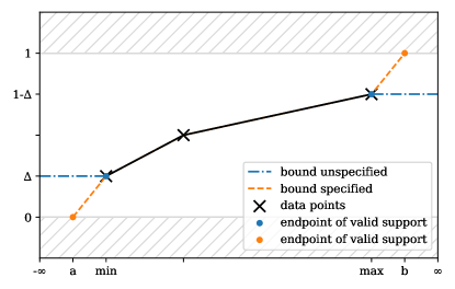
(a) Cumulative distribution function of Algorithm 2

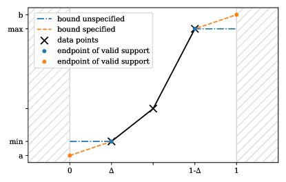
(b) Percent point function of Algorithm 2

Рис. 3: Treating boundary values in Algorithm 2 – The simplest possible example using only 3 data points. Each subfigure shows where the supported values of respective functions map based on whether the boundaries are explicitly set or not. Endpoints denote the ‘‘valid’’ support, i.e. the interval where the function is strictly increasing. E.g., if the boundary $a$ is not set, all CDF values from the interval [$-\infty$, $min$] map to the constant $\Delta=1/(bins+1)$. The PPF maps values from the interval [0, $\Delta$] to $min$, i.e. the minimum value of the provided data. Analogously, the same applies for the boundary value $b$, which can be specified or not independently of $a$.

Estimating a CDF outside of the range of the available samples is a well-known problem as it amounts to extrapolating beyond the observed data. In particular it is already quite difficult to estimate the support of the distribution from which the samples are taken. We deal with this in the following way.
Let $min$ and $max$ denote the smallest resp. largest value of the $n$ samples that were used to generate the Learned Distribution with Algorithm 2, and write $\Delta=1/(bins+1)$. Then, the CDF always maps inputs in $[min,max]$ to values in $[\Delta,1-\Delta]$ and on these intervals the CDF and PPF are inverses of each other. A choice becomes necessary for inputs outside of these intervals. In case the upper or lower boundary of the support of the distribution is known it can be specified as $a$ resp. $b$, in which case the CDF will take the value $0$ at $a$ and $1$ at $b$ and be linear on the intervals $[a,min]$ and $[max,b]$. In this case the CDF and PPF will be inverses of each other on the interval $[a,b]$ resp. $[0,1]$. In this case the CDF will not accept inputs smaller than $a$ or larger than $b$.
If one does not want to make a choice about the assumed support of the distribution, the boundaries can be left unspecified in which case the CDF will simply map all inputs smaller than $min$ to $\Delta$ resp. all inputs larger than $max$ to $1-\Delta$. Similarly, the PPF will map all inputs in $[0,\Delta]$ to $min$ resp. all inputs in $[1-\Delta,1]$ to $max$. This option is essentially saying that we do not expect to receive inputs to the CDF, which are outside of those we have already seen, but in case we do happen to receive such inputs we do not want to extrapolate since this might lead the Redistributor transformation to produce unreasonably large outputs, depending on the target PPF. This may cause issues, for example, in the case of the target being a Gaussian distribution, where the PPF tends to $\pm\infty$ very quickly as the input gets close to $1$ resp. $0$. It is possible to only specify either $a$ or $b$ and leave the other unspecified.
In case of Algorithm 3, the situation is simpler due to the fact that it uses the Gaussian kernel to estimate the density, which has a natural tail behaviour.

3.4 Time & Space Complexity

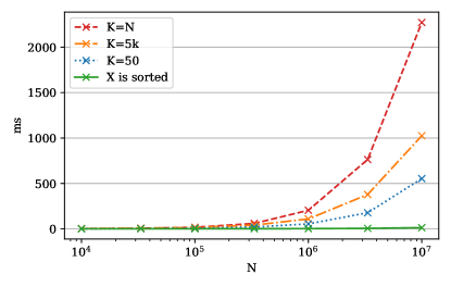
(a) Timing Algorithm 2 – LearnedDistribution

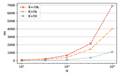
(b) Timing Algorithm 3 – KernelDensity

Рис. 4: Timing algorithms 2 and 3 on consumer grade CPU – Intel ®  Core™ i7-8565U 1.80GHz. In both subfigures, N denotes the number of input data points. In (a), K denotes the number of bins and in (b), K denotes the grid density. Note that in comparison to Algorithm 3, Algorithm 2 can handle approx. 4 orders of magnitude more data points in the same amount of time making it applicable in larger data-processing pipelines.

The time complexity of Algorithm 2 in the worst case is $\mathcal{O}(N\log K)$, where $N$ is the number of data points and $K$ is the number of bins. The bottleneck is partial sorting the data with introspective sort [10] to get the lattice values. In the best case, the input array is already sorted and the time complexity is $\mathcal{O}(N)$. In the worst case $K=N$ and we need to do a full sort instead of a partial sort. In case the lattice values contain repeated values a call to make_unique will add $\mathcal{O}(K\log(K))$. Computation time as a function of $N$ on a specific hardware is shown in Figure 4(a).

The space complexity of Algorithm 2 is $\mathcal{O}(N)$. Auxiliary space complexity is $\mathcal{O}(N)$ if $keep\_x\_unchanged=False$, and $\mathcal{O}(K)$ otherwise. In practical terms, when we use a 1 GB input array, the peak memory will be approx. 2 GB if we want to keep the order of elements in the input array unchanged. If changing the order is not a problem, the peak memory will be approx. 1 GB (not counting the negligible overhead costs of the interpreter, loaded modules, and K-sized arrays stored in the interpolants), i.e. almost no additional memory is used. Being aware of space complexity of this algorithm is important, as its speed allows us to process reasonably large amounts of data points for it to be relevant.

The time complexity of Algorithm 3 is $\mathcal{O}(NK)$ where $N$ is the number of data points and $K$ is the grid density. Most of the time is spent on $N$ evaluations of the Gaussian CDF on $K$-many points. However, evaluating the $cdf$ on $K$ points is vectorized so the speedup depends on particular hardware. Evaluating $ppf$ and $cdf$/fast/ has a time complexity of linear interpolation. Computation time as a function of $N$ on a specific hardware is shown in Figure 4(b).

Space complexity of Algorithm 3 is $\mathcal{O}(N)$. Auxiliary space complexity is $\mathcal{O}(K)$. However, the speed of this algorithm is a limiting factor on the amount of input data points that are reasonable to be processed. Broadly speaking, this algorithm can process approx. 4 orders of magnitude fewer data points than Algorithm 2. With this amount of data, the space complexity is almost always irrelevant.

4 Mathematical Considerations

In this section, we will establish a notion of consistency of the Redistributor transformation generated from an empirical estimator for the CDF of the source distribution, i.e. describe the asymptotic behaviour of $F_{T}^{-1}\circ F^{h}_{n}$ when compared to $F_{T}^{-1}\circ F$, where $F^{h}_{n}$ is our empirical estimator generated from $n$ iid samples of $F$. This will be accomplished by viewing the transformation as a statistical functional on a space containing cumulative distribution functions, and employing what is commonly referred to as the functional delta method. We derive a statement of the form

$$\sqrt{n}(R_{g,x}(F_{n})-R_{g,x}(F))\rightsquigarrow\mathcal{N}(0,\sigma_{g,F,x}),$$

where $\mathcal{N}(0,\sigma_{g,F,x})$ denotes the normal distribution with variance $\sigma_{g,F,x}$ depending on $g$, $F$, and $x$, and $R_{g,x}(F):=(g\circ F)(x)$ describes the output of the transformation for the input $x$. Here $g$ is some function, which in application, would be the PPF $F_{T}^{-1}$ of some target distribution. The statement and the required conditions on $g$, $F$, and $x$ will be made precise in Proposition 4.7. To do so we require a certain amount of technical apparatus (see, e.g., [11]), which we will introduce now.

Definition 4.1.

Let $(X,\|\cdot\|_{X})$, $(Y,\|\cdot\|_{Y})$ be Banach spaces and $D\subseteq X$. A map $\varphi\colon D\to Y$ is called Hadamard differentiable at $F\in D$ if there exists a continuous linear map $\varphi^{\prime}(F)\colon X\to Y$ such that for every $h\in X$, $(h_{n})_{n\in\mathbb{N}}\subseteq X$, $(t_{n})_{n\in\mathbb{N}}\subseteq\mathbb{R}$ with $\lim_{n\to\infty}\|h_{n}-h\|_{X}=0$, $\lim_{n\to\infty}|t_{n}|=0$, and $x+t_{n}h_{n}\in D$, it holds that

$$\lim_{n\to\infty}\|\tfrac{\varphi(F+t_{n}h_{n})-\varphi(F)}{t_{n}}-[\varphi^{\prime}(F)](h)\|_{Y}=0.$$

With this notion of differentiability we can make use of the following theorem.

Theorem 4.2 ([11], Thm.20.8).

Let $(X,\|\cdot\|_{X})$, $(Y,\|\cdot\|_{Y})$ be Banach spaces, $D\subseteq X$ and let $\varphi\colon D\to Y$ be Hadamard differentiable at $F\in X$. Let $G$ and $F_{n}$, $n\in\mathbb{N}$, be $D$-valued random variables and $r_{n}\in\mathbb{R}$, $n\in\mathbb{N}$, with $\lim_{n\to\infty}r_{n}=\infty$. Assume that $r_{n}(F_{n}-F)\rightsquigarrow G$. Then we have

$$r_{n}(\varphi(F_{n})-\varphi(F))\rightsquigarrow[\varphi^{\prime}(F)](G).$$

If $\varphi^{\prime}[F]$ is defined and continuous on the entirety of $X$, we also have

$$r_{n}(\varphi(F_{n})-\varphi(F))=[\varphi^{\prime}[G]](r_{n}(F_{n}-F))+\mathrm{\textbf{o}}_{P}(1).$$

As we are primarily interested in cases where the cumulative distribution function $F$ is continuous and we are generating a continuous empirical cumulative distribution function, a natural Banach space to consider would be $(C_{b}(\mathbb{R},\mathbb{R}),\|\cdot\|)$, i.e. the space of bounded continuous functions from $\mathbb{R}$ to $\mathbb{R}$ equipped with the uniform norm

$$\|f\|_{\infty}:=\sup_{t\in\mathbb{R}}|f(t)|.$$

However in order to derive the desired convergence results, we will need to deal with usual empirical cumulative distribution functions which are discontinuous. Therefore we also introduce the larger space $S=(S,\|\cdot\|_{\infty})$, where

$$S:=\{f\colon\mathbb{R}\to\mathbb{R}\colon\forall x\in\mathbb{R}\colon(\exists\lim_{t\nearrow x}f(t)\wedge\lim_{t\searrow x}f(t)=x\}$$

is the set of functions which are right continuous and have left limits.
We can now consider, for $g\in C((0,1),\mathbb{R})$ and $x\in\mathbb{R}$, the real-valued statistical functional

$$R_{g,x}\colon S_{x} \to\mathbb{R}$$

$$F \mapsto g(F(x)),$$

where

$$S_{x}:=\{F\in S\colon F(x)\in(0,1)\}.$$

The functional $R_{g,x}$ maps a cumulative distribution function $F\in S_{x}$ to the value at $x$ of the Redistributor transformation generated from $g$ and $F$. We consider the inverse cumulative distribution function $g$ as a function on $(0,1)$ and restrict the domain of $R_{g,x}$ to $S_{x}$ in order to avoid the possibility of $g(F(x))\in\{-\infty,\infty\}$. As we have $\mathbb{P}_{x\sim F}[F(x)\in(0,1)]=1$ anyway, this is not a practically relevant restriction. Note that $F\in S_{x}$ if $x$ is in the interior of the suppport of the density function corresponding to $F$. We can now show the following

Lemma 4.3.

Let $g\in C^{1}((0,1),\mathbb{R})$, $x\in\mathbb{R}$, and $F\in S_{x}$. Then the Hadamard derivative of $R_{g,x}$ at $F$ is continuous and given by $[R^{\prime}_{g,x}(F)](h)=g^{\prime}(F(x))h(x)$ for $h\in S$.

Доказательство.

Let $h\in S$, $(h_{n})_{n\in\mathbb{N}}\subseteq S$, $(t_{n})_{n\in\mathbb{N}}\subseteq\mathbb{R}$ with $\lim_{n\to\infty}\|h_{n}-h\|_{\infty}=0$, $\lim_{n\to\infty}|t_{n}|=0$.
Then

$$\left(\tfrac{R_{g,x}(F+t_{n}h_{n})-R_{g,x}(F)}{t_{n}}\right)(x)=\tfrac{g(F(x)+t_{n}h_{n}(x))-g(F(x))}{t_{n}}.$$

The definition of $S_{x}$ ensures $F(x)\in(0,1)$ and therefore continuity of $g$ guarantees the existence of a neighborhood around $F(x)$ on which $g$ is finite. As a direct consequence of the assumptions we have $\lim_{n\to\infty}|t_{n}h_{n}(x)|=0$ and consequently there exists $n_{0}\in\mathbb{N}$ such that $F(x)+t_{n}h_{n}(x)$ is in this neighborhood for all $n\geq n_{0}$. We will assume in the following that $n\geq n_{0}$.
By considering the Taylor expansion of $g$ around $F(x)$ evaluated at $F(x)+t_{n}h_{n}(x)$ we get that

$$g(F(x)+t_{n}h_{n}(x))=g(F(x))+g^{\prime}(F(x))t_{n}h_{n}(x)+r(F(x)+t_{n}h_{n}(x))t_{n}h_{n}(x),$$

where

$$\lim_{n\to\infty}r(F(x)+t_{n}h_{n}(x))=0.$$ (2)

Consequently we get

$$|\tfrac{g(F(x)+t_{n}h_{n}(x))-g(F(x))}{t_{n}}-g^{\prime}(F(x))h(x)| =|g^{\prime}(F(x))h_{n}(x)+r(F(x)+t_{n}h_{n}(x))h_{n}-g^{\prime}(F(x))h(x)|$$

$$\leq|g^{\prime}(F(x))(h_{n}(x)-h(x))|+|r(F(x)+t_{n}h_{n}(x))h_{n}(x)|.$$

Due to (2) and $\lim_{n\to\infty}\|h_{n}-h\|_{\infty}=0$ this implies

$$\lim_{n\to\infty}\left|\tfrac{R_{g,x}(F+t_{n}h_{n})-R_{g,x}(F)}{t_{n}}-g^{\prime}(F(x))h(x)\right|=0,$$

which proves that $[R^{\prime}_{g,x}(F)](h)=g^{\prime}(F(x))h(x)$.
Moreover, $R^{\prime}_{g,x}(F)$ is continuous as, for all $h_{1},h_{2}\in S$, it holds that

$$|R(h_{1})-R(h_{2})|=|g^{\prime}(F(x))h_{1}(x)-g^{\prime}(F(x))h_{2}(x)|\leq|g^{\prime}(F(x))|\ \|h_{1}-h_{2}\|_{\infty}.$$

∎

Note that each empirical cumulative distribution function $F_{n}\in S$ is derived from a real valued random variable with cumulative distribution function $F\in C_{b}(\mathbb{R},\mathbb{R})$ by application of a deterministic function $h^{*}_{n}\colon T^{n}\to S$ to $(X_{1},\dots,X_{n})$, where $X_{i}\sim F$, $i\in\{1,\dots,n\}$, iid and

$$T^{n}:=\{x\in\mathbb{R}^{n}\colon x_{1}<\dots<x_{n}\}.$$

Specifically we have

$$F_{n}(t)=(h^{*}_{n}(X_{\pi(1)},\dots,X_{\pi(n)})(t):=\tfrac{1}{n}\sum_{k=1}^{n}\mathds{1}_{[X_{k}\leq t]},$$

where $(X_{\pi(1)},\dots,X_{\pi(n)})$ is an increasing rearrangement of $(X_{1},\dots,X_{n})$.
Colloquially speaking, the sequence $(h^{*}_{n})_{n\in\mathbb{N}}$ describes the deterministic method to generate the usual empirical cumulative distribution function out of $n$ of real-valued samples from $F$. In this functional setting the convergence of the empirical cumulative distributions functions can be described by the following Theorem from [11].

Theorem 4.4.

Let $F\in S$ be the cumulative distribution function of a real-valued random variable and $(F_{n})_{n\in\mathbb{N}}$ the corresponding sequence of empirical cumulative distribution functions. Then we have

$$\sqrt{n}(F_{n}-F)\rightsquigarrow\mathbb{G}_{F},$$ (3)

i.e. convergence in distribution in the space $(S,\|\cdot\|_{\infty})$, where $\mathbb{G}_{F}$ is a zero-mean Gaussian process with covariance

$$\mathrm{cov}[\mathbb{G}_{F}(s),\mathbb{G}_{F}(t)]=\min\{F(s),F(t)\}-F(s)F(t).$$

Our algorithm, however, generates a continuous empirical distribution function out of a vector of samples $(X_{1},\dots,X_{n})$. We therefore need to consider what conditions on a sequence $h=(h_{n})_{n\in\mathbb{N}}$ of functions $h_{n}\colon T^{n}\to S$ are required to ensure that (3) remains valid. More precisely, we write

$$F^{h}_{n}:=h_{n}(X_{\pi(1)},\dots,X_{\pi(n)})\in S$$

for the function-valued random variable derived by the deterministic function $h_{n}$ from the real-valued cumulative distribution function $F\in C_{b}(\mathbb{R},\mathbb{R})$. This is done via taking $X_{i}\sim F$, $i\in\{1,\dots,n\}$, iid, where, again, $(X_{\pi(1)},\dots,X_{\pi(n)})$ is an increasing rearrangement of $(X_{1},\dots,X_{n})$. We them need to show that with this construction, we still obtain

$$\sqrt{n}(F^{h}_{n}-F)\rightsquigarrow\mathbb{G}_{F},$$

To accomplish this we will make use of a continuous mapping theorem for Banach-space-valued random variables.

Theorem 4.5 ([11], Thm.18.11).

Let $(D,\|\cdot\|_{D})$, $(E,\|\cdot\|_{E})$ be Banach spaces. Assume that $D_{n}\subseteq D$ and $g_{n}\colon D_{n}\to E$, $n\in\mathbb{N}\cup\{\infty\}$, satisfy for every sequence $(x_{n})_{n\in\mathbb{N}}$ with $x_{n}\in D_{n}$, that for every subsequence $(x_{n_{k}})_{k\in\mathbb{N}}\subseteq\mathbb{N}$ we have

$$\Big{(}\exists s\in D_{\infty}\colon\lim_{k\to\infty}\|x_{n_{k}}-s\|_{D}=0\Big{)}\implies\lim_{k\to\infty}\|g_{n_{k}}(x_{n_{k}})-g_{\infty}(s))\|_{E}=0.$$

Then, for any sequence of random variables $X_{n}\in D_{n}$, $n\in\mathbb{N}$, and random variable $X\in D_{\infty}$ with $g_{\infty}(X)\in E$, it holds that

$$X_{n}\rightsquigarrow X\implies g_{n}(X_{n})\rightsquigarrow g_{\infty}(X).$$

We obtain the following Lemma, which essentially states that, if a deterministic construction method $(h_{n})_{n\in\mathbb{N}}$ is sufficiently close to the one of the usual empirical cumulative distribution function, i.e. $(h^{*}_{n})_{n\in\mathbb{N}}$, then the corresponding sequences of function-valued random variables $(F^{h}_{n})_{n\in\mathbb{N}}$ and $(F_{n})_{n\in\mathbb{N}}$ enjoy the same kind of convergence.

Lemma 4.6.

Let $F\in C_{b}(\mathbb{R},\mathbb{R})$ be the cumulative distribution function of a real-valued random variable and $h_{n}\colon T^{n}\to S$, $n\in\mathbb{N}$, a sequence of functions. Assume that there exist constants $C>0$ and $c>\tfrac{1}{2}$ such that for all $n\in\mathbb{N}$, $x\in\mathbb{R}^{n}$ it holds that

$$\|h_{n}(x)-h^{*}_{n}(x)\|_{\infty}\leq Cn^{-c}.$$ (4)

Then we have

$$\sqrt{n}(F^{h}_{n}-F)\rightsquigarrow\mathbb{G}_{F},$$

where $\mathbb{G}_{F}$ is a zero-mean Gaussian process with covariance

$$\text{cov}[\mathbb{G}_{F}(s),\mathbb{G}_{F}(t)]=\min\{F(s),F(t)\}-F(s)F(t).$$

Доказательство.

This proof is effected by a fairly straightforward application of Theorem 4.5. To this end, let $D=D_{\infty}=E=(S,\|\cdot\|_{\infty})$ and, for $n\in\mathbb{N}$,

$$D_{n}:=\{\widetilde{x}\in S\colon x\in T^{n}\},$$

where

$$\widetilde{x}(t):=\sqrt{n}\big{(}F(t)-\tfrac{1}{n}\sum_{k=1}^{n}\mathds{1}_{[x_{k}\leq t]}\big{)}=\sqrt{n}\big{(}F(t)-(h^{*}_{n}(x))(t)\big{)},\quad\quad x\in T^{n},t\in\mathbb{R}.$$

In particular we have that $\sqrt{n}(F_{n}-F)$ is a random variable in the function space $D_{n}\subseteq S$. Moreover, the map $T^{n}\ni x\mapsto\widetilde{x}\in D_{n}$ is bijective since $F$ is continuous, which means that the points of discontinuity of $\widetilde{x}$ uniquely determine $x$. Therefore there are well-defined maps $g_{n}\colon D_{n}\to S$, $n\in\mathbb{N}$, which satisfy for all $n\in\mathbb{N}$, $\widetilde{x}\in D_{n}$, that

$$g_{n}(\widetilde{x})=\sqrt{n}(F-h_{n}(x)).$$

We will show that the requirement in Theorem 4.5 is satisfied with $g_{\infty}\colon S\to S$ being the identity. To this end consider $(\widetilde{x}_{n})_{n\in\mathbb{N}}$ with $\widetilde{x}_{n}\in D_{n}$ and assume there exists a subsequence $(\widetilde{x}_{n_{k}})_{k\in\mathbb{N}}$ and $s\in S$ such that

$$\lim_{k\to\infty}\|\widetilde{x}_{n_{k}}-s\|_{\infty}=0.$$ (5)

We have

$$\|g_{n_{k}}(\widetilde{x}_{n_{k}})-g_{\infty}(s)\|_{\infty} =\|\sqrt{n_{k}}(F-h_{n_{k}}(x_{n_{k}}))-s\|_{\infty}$$

$$=\|\sqrt{n_{k}}(F-h_{n_{k}}(x_{n_{k}})+h^{*}_{n_{k}}(x_{n_{k}})-h^{*}_{n_{k}}(x_{n_{k}}))-s\|_{\infty}$$

$$\leq\sqrt{n_{k}}\|h_{n_{k}}(x_{n_{k}})-h^{*}_{n_{k}}(x_{n_{k}})\|_{\infty}+\|\sqrt{n_{k}}(F-h^{*}_{n_{k}}(x_{n_{k}}))-s\|_{\infty}.$$

The first term vanishes for $k\to\infty$ as we assumed $c>\tfrac{1}{2}$ and

$$\sqrt{n_{k}}\|h_{n_{k}}(x_{n_{k}})-h^{*}_{n_{k}}(x_{n_{k}})\|_{\infty}\leq Cn_{k}^{\frac{1}{2}-c},$$

whereas the second term vanishes for $k\to\infty$ due to assumption (5). Consequently we have

$$\lim_{k\to\infty}\|g_{n_{k}}(\widetilde{x})-g_{\infty}(s)\|_{\infty}=0$$

as claimed. Note that

$$g_{n}(\sqrt{n}(F_{n}-F)) =g_{n}(\sqrt{n}(F-h^{*}_{n}(X_{\pi(1)},\dots,X_{\pi(n)})))$$

$$=\sqrt{n}(F-F^{h}_{n}(X_{\pi(1)},\dots,X_{\pi(n)}))$$

$$=\sqrt{n}(F^{h}_{n}-F).$$

Since $\sqrt{n}(F_{n}-F)\rightsquigarrow\mathbb{G}_{F}$ by Theorem 4.4, application of Theorem 4.5 yields $\sqrt{n}(F^{h}_{n}-F)\rightsquigarrow\mathbb{G}_{F}$, which completes the proof. ∎

We next argue that the constructions $(h_{n})_{n\in\mathbb{N}}$ we use to obtain the continuous empirical distribution function fulfill condition (4). We first observe that for $n\in\mathbb{N}$ and $x\in T^{n}$, the functions $(h_{n})_{n\in\mathbb{N}}$ satisfy

$$(h_{n}(x))(t)\in[0,\tfrac{1}{n+1}] \mathrm{for}\ t\leq x_{1},$$

$$(h_{n}(x))(t)\in[\tfrac{n}{n+1},1] \mathrm{for}\ t\geq x_{n},$$

$$(h_{n}(x))(x_{k})=\tfrac{k}{n+1} \mathrm{for}\ k\in[n],$$

and are linear on each interval $[x_{k},x_{k+1}]$ for $k\in\{1,\dots,n-1\}$. We therefore have for $n\in\mathbb{N}$, $x\in T^{n}$, $k\in\{1,\dots,n-1\}$, $t\in[x_{k},x_{k+1})$ that

$$|(h_{n}(x))(t)-(h^{*}_{n}(x))(t)| \leq|(h_{n}(x))(t)-(h_{n}(x))(x_{k})|+|(h_{n}(x))(x_{k})-(h^{*}_{n}(x))(t)|$$

$$\leq|(h_{n}(x))(x_{k+1})-(h_{n}(x))(x_{k})|+|(h_{n}(x))(x_{k})-(h^{*}_{n}(x))(x_{k})|$$

$$\leq\tfrac{1}{n+1}+(\tfrac{k}{n}-\tfrac{k}{n+1})$$

$$\leq 2n^{-1}.$$

Moreover, we have for $t<x_{1}$ that $|(h_{n}(x))(t)-(h^{*}_{n}(x))(t)|=|(h_{n}(x))(t)|\leq|(h_{n}(x))(x_{1})|=\tfrac{1}{n+1}$ and for $t\geq x_{n}$ that $|(h_{n}(x))(t)-(h^{*}_{n}(x))(t)|=|1-(h_{n}(x))(t)|\leq|1-(h_{n}(x))(x_{1})|=\tfrac{1}{n+1}$. As such, our construction satisfies (4) and is covered by the following proposition.

Proposition 4.7.

Let $g\in C^{1}((0,1),\mathbb{R})$, $x\in\mathbb{R}$, $F\in S_{x}$, and $h=(h_{n})_{n\in\mathbb{N}}$ such that the assumptions of Lemma 4.6 are satisfied. Then

$$\sqrt{n}(R_{g,x}(F^{h}_{n})-R_{g,x}(F))\rightsquigarrow g^{\prime}(F(x))\mathbb{G}_{F}(x)=\mathcal{N}\big{(}0,(g^{\prime}(F(x)))^{2}(F(x)-F(x)^{2})\big{)}.$$

Доказательство.

Lemma 4.6 ensures $\sqrt{n}(F^{h}_{n}-F)\rightsquigarrow\mathbb{G}_{F}$ and thus Theorem 4.2 yields

$$\sqrt{n}(R_{g,x}(F^{h}_{n})-R_{g,x}(F))\rightsquigarrow[R^{\prime}_{g,x}(F)](\mathbb{G}_{F}(x)).$$

Due to Lemma 4.3 we further have

$$[R^{\prime}_{g,x}(F)](\mathbb{G}_{F}(x)) =g^{\prime}(F(x))\mathbb{G}_{F}(x)$$

$$=g^{\prime}(F(x))\mathcal{N}\big{(}0,F(x)-F(x)^{2}\big{)}$$

$$=\mathcal{N}\big{(}0,(g^{\prime}(F(x)))^{2}(F(x)-F(x)^{2})\big{)}.$$

∎

4.1 Componentwise Application to Multi-dimensional Random Variables

So far we have analyzed the behaviour of the Redistributor transformation using an empirical estimator generated with iid samples from some real-valued random variable. We could however also consider a vector-valued random variable $X\in\mathbb{R}^{d}$. Given samples $X^{i}\sim X$, $i\in[n]$, one can consider the collection of scalar values $(X^{i}_{j})_{i\in[n],j\in[d]}\subseteq\mathbb{R}$ and take the empirical cumulative distribution function $h^{*}_{nd}((X^{i}_{j})_{i\in[n],j\in[d]})$ as if it was a vector of samples from a real-valued random variable. We note that

$$(h^{*}_{nd}((X^{i}_{j})_{i\in[n],j\in[d]}))(t)=\tfrac{1}{nd}\sum_{j\in[d]}\sum_{i\in[n]}\mathds{1}_{[X^{i}_{j}\leq t]}=\tfrac{1}{d}\sum_{j\in[d]}h^{*}_{n}((X^{i}_{j})_{i\in[n]}).$$

Which means this would be the empirical cumulative distribution function of a scalar-valued random $\widetilde{X}$ variable with cumulative distribution function $\widetilde{F}=\tfrac{1}{d}\sum_{j\in[d]}F_{j}$ with $F_{j}$ being the cumulative distribution function of $X_{j}\in\mathbb{R}$. Similarly taking our empirical estimator to get $\widetilde{F}^{h}_{n}=h_{n}((X^{i}_{j})_{i\in[n],j\in[d]}))$ would yield an approximation, in the sense of Proposition 4.7, of the transformation $\widetilde{R}$ which satisfies

$$\widetilde{R}(\widetilde{X})\overset{\text{d}}{=}Y,$$

where $Y$ is a random variable with cumulative distribution function $g$. While the statistical implications of applying a thusly created transformation component-wise to a vector $x\in\mathbb{R}^{d}$, is quite unclear, this type of use of the Redistributor transformation to, e.g. images, yields some appealing results as can be seen in the next section.

5 Use Cases

Transforming data to approximately normal has long been used as a statistical preprocessing step. The additional flexibility provided by Redistributor, however, allows for novel applications, e.g., in image processing and data augmentation.

5.1 Matching Exposure in Photography

Poorly lit or under/over-exposed photos are a common occurrence, so much so that photo editing programs have automated tool for correcting this. Redistributor can greatly outperform these built-in tools by switching an "auto-color"or "brightening/darkening"tool to one that will match the color distribution of a properly exposed photo. As seen in Figure 5 the entire range of colors can be matched properly by providing a reference for what the photo should look like had it been properly exposed.

While other tools either operate on the exposure of the whole image, or light/dark regions separately, Redistributor modifies the distribution of pixel values to match. Note that this does more than merely add light to the example photo, but also corrects colors. Redistributor was used on each channel of the color image separately resp. on the single channel of the gray-scale image. Each channel was redistributed separately to match (in distribution) that of the target photograph.

(a) Underexposed RGB (source)

(b) Underexposed GRAY (source)

(c) Well-exposed RGB (target)

(d) Well-exposed GRAY (target)

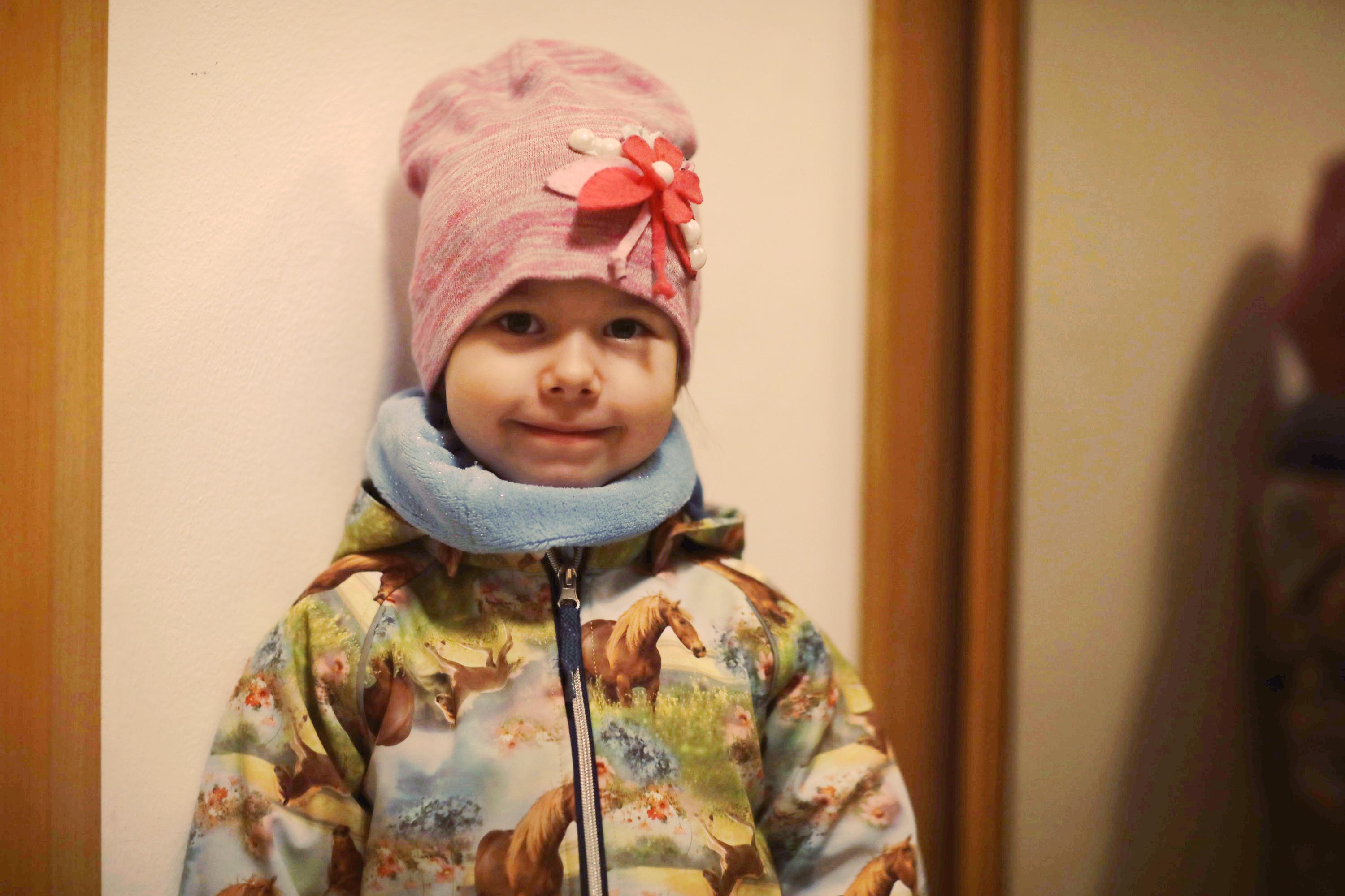
(e) Corrected RGB (our method)

(f) Corrected GRAY (our method)

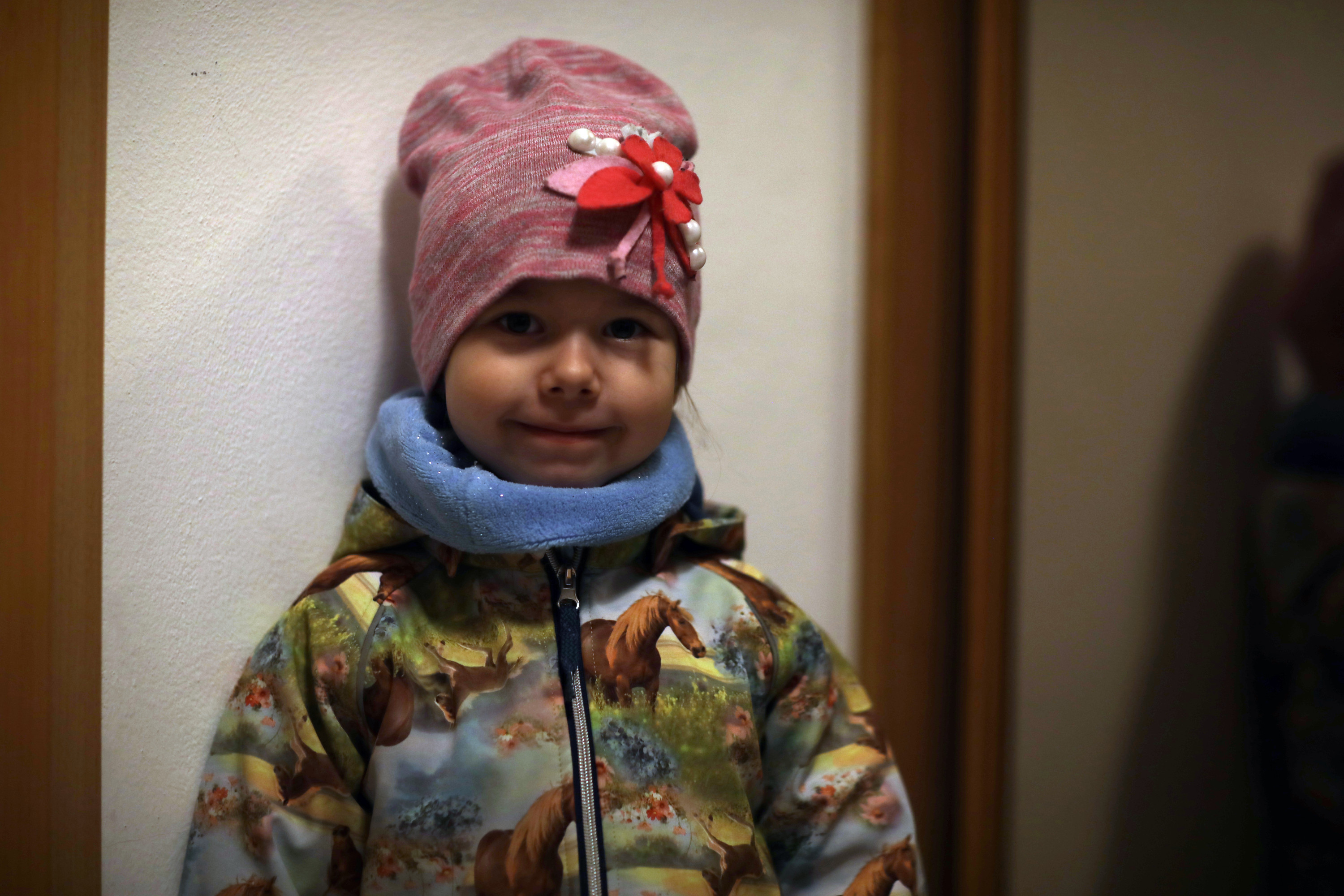
(g) Corrected RGB (Photopea.com auto-color)

(h) Corrected GRAY (Photopea.com auto-color)

Рис. 5: Correcting bad exposure using a reference image.

5.2 Matching Colors of a Reference Image

Moving in the direction of AI augmented art, we consider the translation or recreation of a photo in a modified color scheme. Figure 6 illustrates several examples. The first example, that of an evening photo turned into a "sunset"photo is most closely related to the previous subsection: under/over-exposed photographs can capture wildly different colors, e.g., when photographing a sunset.

Even when the desired photo is captured, as in the remaining three rows, great effects can be produced by translating the color scheme to a desired distribution. This can be used to not only create surreal images as in subfigure (f), but also to create consistent color schemes for design or decoration.

(a) Source

(b) Target

(c) Output (our method)

(d) Source

(e) Target

(f) Output (our method)

(g) Source

(h) Target

(i) Output (our method)

(j) Source

(k) Target

(l) Output (our method)

Рис. 6: Matching colors of a reference image.

5.3 Making Photomosaics

As a further use case in image modification, Redistributor can easily make photographic mosaics (photomosaics). These are images that have been divided into smaller, tiled regions, each of which is replaced by an image with similar mean color value as the original tile. Usually, mosaics are created by selecting the smaller images from a large collection. The resulting granularity is a function of both the size of the collection as well as the size of the tiles. Redistributor instead transforms any provided image to a Gaussian distribution with mean $\mu$ matching the tile to replace. By doing so, one could even make a mosaic by repeatedly using only a single image. Furthermore, the granularity of the mosaic can be easily modified using a parameter $\sigma$ of the target Gaussian distribution, either keeping or compressing the variability in an individual sub-image. Moreover, the original full-resolution image can be overlaid over the mosaic to regain high-frequency content, adding another parameter $\alpha$ influencing the ratio between the mosaic and the original image it depicts. Examples of mosaics created with varying parameters are shown in Figure 7.

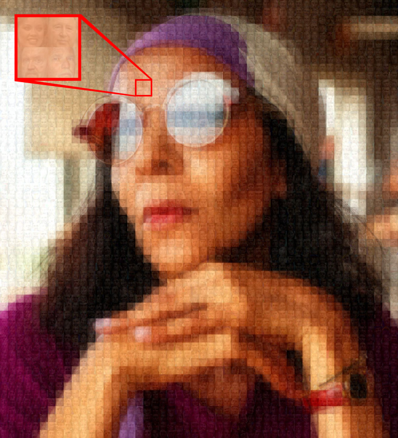
(a) Mosaic 1 – $50\times 50$ mosaic made of 1000 px² tiles redistributed to a Gaussian with $\mu=$ desired pixel value and $\sigma=0.05$. The original image is overlaid over the mosaic with $\alpha=0.25$ to regain high-frequency content.

(b) $\alpha=0.00$, $\sigma=0.05$

(c) $\alpha=0.25$, $\sigma=0.20$

(d) $\alpha=0.25$, $\sigma=0.40$

Рис. 7: Mosaic effect achieved by tiling redistributed images from the LFW dataset [12].

5.4 Image Data Augmentation in Colorspace

Redistributor may also be used for Image data augmentation in colorspace, as described in [13], i.e. taking an image and producing a similar one by modifying the histograms of the RGB color channels. Figure 8 illustrates the example of a batch of $6$ images, where out of each image $5$ new ones have been created by channel-wise redistribution to match each of the other images. One can also create new versions of an image by redistributing them to some manually chosen distribution of interest, depending on the specifics of the intended application. Naturally, Redistributor could also be applied to any other type of data as long as it consists of some collection of scalar values. Of course, it is not always clear whether these augmentations are necessarily sensible for the intended task. While the benefits and drawbacks need to be carefully considered based on the goals of the intended application, Redistributor always provides an efficient and flexible tool for systematic data augmentation.

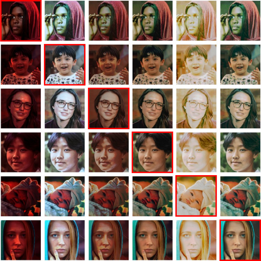
Рис. 8: Augmenting image data in color space using distributions of other images within the same batch. The original images are highlighted using a red border. All images within one column are redistributed according to the image in the same column that lies on the diagonal. E.g. image in row 3, column 2 is redistributed according to the image in row 2, column 2.

5.5 Preprocessing for Machine Learning Tasks

Another potential application of this algorithm would be as a preprocessing step for machine learning tasks. It is designed to efficiently handle a large number of samples with a low memory footprint, and as it is implemented as a Scikit-learn transformer, it can be conveniently inserted in common machine learning pipelines. It always produces an invertible transformation, i.e. does not, in principle, reduce the input-output relationships which may be learned. In addition, Section 4 shows that given $n$ iid samples of a CDF $F_{S}$ and some specified target CDF $F_{T}$, it is a consistent estimator of $F_{T}^{-1}\circ F_{S}$, i.e. it can be expected to behave predictably on further samples of $F_{S}$. Particularly when applied component-wise to high-dimensional data, e.g. images, it seems unlikely that it would improve things from a statistical perspective. However, there might be other benefits. For example, when the source distribution is very highly concentrated around some small value, it could serve as a kind of normalization and lead to improved numerical performance of an algorithm.
Anecdotally, we have observed various cases of improved performance on a number machine learning tasks using neural networks. The improvement is, however, not very consistent and often rather mild. Although, given the simple and inexpensive nature of this preproccesing step it would be quite unreasonable to expect a consistent significant improvement anyway. We abstain from presenting numerical examples for this use case, since this is not the focus of the paper and the black-box nature of neural networks means that a brief demonstration would require significant cherry picking.

5.6 Connection to Transport Based Signal Processing

So far we have been interested in the output we can obtain by applying the Redistributor transformation $R$ to some input of interest. To round out this section we will briefly mention a rather different usage of the basic idea behind the Redistributor, which has been put forward in [14]. We give a somewhat simplified and slightly paraphrased description.
Let $f\colon\mathbb{R}\to\mathbb{R}$ be a continuous function with $\|f\|_{1}:=\int_{\mathbb{R}}f(x)\mathrm{d}x=1$, i.e. such that we can interpret it as a density function, and let $F_{T}=\int_{-\infty}^{x}f(x)\mathrm{d}x$ denote the corresponding CDF. Moreover we fix some reference probability measure with continuous density function $f_{S}$ and CDF $F_{S}$. We can now consider the so-called Cumulative Distribution Transform $\hat{f}\colon\mathbb{R}\to\mathbb{R}$ of $f$, which can be written as

$$\hat{f}(x)=(R(x)-x)\sqrt{f_{s}(x)},$$

where $R=F_{T}^{-1}\circ F_{S}$ is simply the Redistributor transformation. In this setting one considers data $(f_{i})_{i\in\mathbb{N}}$ where each $f_{i}$ can be represented suitably as a function. In [14] a number of advantages of applying the CDT to each of the data points and working with the set $(\hat{f}_{i})_{i\in\mathbb{N}}$ are shown theoretically and demonstrated empirically. This has been developed into a number of interesting methods for signals processing, see [15].

6 Discussion

We present a fully-fledged package which implements a theoretically supported method for transforming one data distribution to another. We refer to this process to as "redistribution"and hence our Python package is called Redistributor. The flexibility that we provide allows for the exploration of many machine learning tasks such as image processing and data preprocessing. As our transformation is based on ranks, there isn’t a sincere benefit to using Gaussian-based inference on the transformed data as opposed to rank-based inference. Convenience could be gained, however, and our theoretical results could be used to support the asymptotics of such tests. In some situations where the learned transformation between distributions is stable, one could also use Redistributor in transfer learning, either as a preprocessing tool or to estimate the model in one domain and redistribute them to another. Such tasks are the focus of future work.

- [1] G. E. P. Box and D. R. Cox. An analysis of transformations. Journal of the Royal Statistical Society: Series B (Methodological), 26(2):211–243, 1964. doi:10.1111/j.2517-6161.1964.tb00553.x.
- [2] M. R. Peltier, C. J. Wilcox, and D. C. Sharp. Technical note: Application of the Box-Cox data transformation to animal science experiments. Journal of Animal Science, 76(3):847–849, 03 1998. doi:10.2527/1998.763847x.
- [3] J. Osborne. Improving your data transformations: Applying the Box-Cox transformation. Practical Assessment, Research, and Evaluation, 15(12), 2010. doi:10.7275/qbpc-gk17.
- [4] M. S. Bartlett. The use of transformations. Biometrics, 3(1):39–52, 1947. doi:10.2307/3001536.
- [5] Ryan A. Peterson. Finding Optimal Normalizing Transformations via bestNormalize. The R Journal, 13(1):310–329, 2021. doi:10.32614/RJ-2021-041.
- [6] R Core Team. R: A Language and Environment for Statistical Computing. R Foundation for Statistical Computing, Vienna, Austria, 2022. URL: https://www.R-project.org/.
- [7] Luc Devroye. Nonuniform random variate generation. Handbooks in operations research and management science, 13:83–121, 2006. doi:10.1016/S0927-0507(06)13004-2.
- [8] Yen-Chi Chen. A tutorial on kernel density estimation and recent advances. Biostatistics & Epidemiology, 1(1):161–187, 2017. doi:10.1080/24709360.2017.1396742.
- [9] F. Pedregosa, G. Varoquaux, A. Gramfort, V. Michel, B. Thirion, O. Grisel, M. Blondel, P. Prettenhofer, R. Weiss, V. Dubourg, J. Vanderplas, A. Passos, D. Cournapeau, M. Brucher, M. Perrot, and E. Duchesnay. Scikit-learn: Machine learning in Python. Journal of Machine Learning Research, 12:2825–2830, 2011.
- [10] David R Musser. Introspective sorting and selection algorithms. Software: Practice and Experience, 27(8):983–993, 1997.
- [11] A. W. van der Vaart. Asymptotic Statistics. Cambridge Series in Statistical and Probabilistic Mathematics. Cambridge University Press, 1998. doi:10.1017/CBO9780511802256.
- [12] Gary B. Huang, Manu Ramesh, Tamara Berg, and Erik Learned-Miller. Labeled faces in the wild: A database for studying face recognition in unconstrained environments. Technical Report 07-49, University of Massachusetts, Amherst, October 2007. URL: http://vis-www.cs.umass.edu/lfw/.
- [13] Connor Shorten and Taghi M Khoshgoftaar. A survey on image data augmentation for deep learning. Journal of big data, 6(1):1–48, 2019. doi:10.1186/s40537-019-0197-0.
- [14] S. Park, S. Kolouri, S. Kundu, and G. Rohde. The cumulative distribution transform and linear pattern classification. Applied and Computational Harmonic Analysis, 45, 2015. doi:10.1016/j.acha.2017.02.002.
- [15] A. H. M. Rubaiyat, M. S. E. Rabbi, L. Cattell, X. Yin, S. Li, Y. Zhuang, G. Rohde, S. Kolouri, and S. Park. PyTransKit. https://github.com/rohdelab/PyTransKit.