Unit Averaging
for Heterogeneous Panels

Abstract

In this work we introduce a unit averaging procedure to efficiently recover unit-specific parameters in a heterogeneous panel model. The procedure consists in estimating the parameter of a given unit using a weighted average of all the unit-specific parameter estimators in the panel. The weights of the average are determined by minimizing an MSE criterion. We analyze the properties of the minimum MSE unit averaging estimator in a local heterogeneity framework inspired by the literature on frequentist model averaging. The analysis of the estimator covers both the cases in which the cross-sectional dimension of the panel is fixed and large. In both cases we obtain the local asymptotic distribution of the minimum MSE unit averaging estimators and of the associated weights. A GDP nowcasting application for a panel of European countries showcases the benefits of the procedure.

Keywords: heterogeneous panels, frequentist model averaging, prediction

JEL: C33, C52, C53

1 Introduction

Estimation of unit-specific parameters in panel data models with heterogeneous parameters is a topic of active research in econometrics (Maddala et al., 1997; Pesaran et al., 1999; Wang et al., 2019; Liu et al., 2020). Estimation of unit-specific parameters is relevant, for instance, when interest lies in constructing forecasts for the individual units in the panel (Baltagi, 2013; Zhang et al., 2014; Wang et al., 2019; Liu et al., 2020), which typically arises in the analysis of international panels of macroeconomic time series (Marcellino et al., 2003). Other unit-specific parameters of interest include individual slopes (Maddala et al., 1997, 2001; Wang et al., 2019) and long-run effects of a change in a covariate (Pesaran and Smith, 1995; Pesaran et al., 1999).

There are three natural strategies for estimating unit-specific parameters (Baltagi et al., 2008). The simplest approach consists in estimating each unit-specific parameter from its individual time series. While this strategy typically leads to approximately unbiased estimation, the resulting estimators suffer from large estimation variability when the time dimension is small. In the second approach, an assumption of parameter homogeneity is imposed and a common panel-wide estimator is used for all unit-specific parameters. This strategy leads to small variability; however, it suffers from large bias in the presence of heterogeneity. The third strategy is a compromise between the first two. It combines pooled and individual approaches in the attempt to obtain an estimator with favorable risk properties (Maddala et al., 2001; Wang et al., 2019; Liu et al., 2020). This is appealing when the time dimension is moderate and there is a nontrivial bias-variance trade-off between individual-specific and panel-wide estimation.

In this paper we propose a novel unit-specific compromise estimator that we call the unit averaging estimator. The estimator is fairly general and is designed for possibly nonlinear panel models estimated by M-estimation. We are concerned with the estimation of a unit-specific “focus” parameter. Focus parameters considered include the examples mentioned above as well as other smooth transformations of the unit-specific parameter vector. The unit averaging estimator for the unit-specific focus parameter is then defined as a weighted average of all the unit-specific focus parameter estimators in the panel. The weights of the average are chosen by minimizing a unit-specific MSE criterion. Specifically, we introduce two MSE criteria that differ in whether the cross-sectional dimension of the panel is treated as fixed (fixed-$N$) or large (large-$N$). The minimum MSE weights solve a quadratic optimization problem that is straightforward to compute in both approaches.

We analyze the theoretical properties of the proposed unit averaging methodology. The analysis is carried out using a local heterogeneity assumption, in which we assume that individual coefficients are local in the time dimension to a common mean. This is inspired by and builds upon the notion of local misspecification used in the frequentist model averaging literature (Hjort and Claeskens, 2003; Claeskens and Hjort, 2008; Hansen, 2008). Local heterogeneity may be interpreted as a theoretical device to emulate panels where the time dimension is moderate. In such a setting each unit carries information about the other units in the panel and thus may improve estimation accuracy. Using the local heterogeneity framework we derive the local asymptotic MSE of the unit averaging estimator as well as estimators for this quantity. The minimum MSE weights minimize the local asymptotic MSE estimators. As we show, these minimum MSE weights minimize an appropriately defined notion of the asymptotic MSE contaminated by a noise component that we characterize explicitly. Finally, we obtain the limiting distribution of the minimum MSE unit averaging estimator similarly to Liu (2015).

In a simulation study, we assess the finite sample properties of the proposed methodology. We compare our unit averaging estimator against the unit-specific estimator, the mean group estimator as well as alternative unit averaging estimators based on AIC weights, BIC weights and Mallows weights (Buckland et al., 1997; Hansen, 2007; Wan et al., 2010). The simulation study shows that the proposed methodology performs favorably relative to these benchmarks. The improvement in MSE is strongest for those units whose individual parameter is sufficiently distant from both the mean of the distribution and the endpoints of the support.

An application to GDP nowcasting for a panel of European countries showcases the methodology (Marcellino and Schumacher, 2010; Schumacher, 2016). GDP prediction is a natural application of the unit averaging methodology since the literature documents both evidence of heterogeneity between countries and the benefits of pooling data (Garcia-Ferrer et al., 1987; Hoogstrate et al., 2000; Marcellino et al., 2003). We find that unit averaging using minimum MSE weights improves prediction accuracy and that the magnitude of the improvement is larger for shorter panels.

This paper is related to different strands of the literature. First, it is related to the literature on frequentist model averaging. Important contributions in this area include Hjort and Claeskens (2003), Hansen (2007), Hansen (2008), Wan et al. (2010), Hansen and Racine (2012), Liu (2015), and Gao et al. (2016), among others. Gao et al. (2016); Yin et al. (2021) deal with model averaging estimators specifically tailored for panel models. The main difference with respect to these contributions is that we focus on averaging different units with the same model whereas these papers average different models. Second, this paper is related to the literature on unit-specific estimation using compromise estimators. Important contributions in this area include Zhang et al. (2014), Wang et al. (2019), Issler and Lima (2009) and Liu et al. (2020). The main difference with respect to these contributions is that we focus on a setting where the time dimension is moderate (as opposed to either large or small) and that we do not require strict exogeneity. Moreover, the existing literature largely focuses on linear models (Baltagi et al., 2008; Wang et al., 2019) whereas our framework allows for a large class of nonlinear models.

The rest of the paper is structured as follows. Section 2 introduces the unit averaging methodology. Section 3 studies the theoretical properties of the procedure. Section 4 contains the simulation study. Section 5 contains the empirical application. Concluding remarks follow in section 6. All proofs are collected in the proof appendix. Additional results are collected in the online appendix, available from the authors’ websites.

2 Methodology

We introduce our unit averaging methodology within the framework of a fairly general class of panel data models with heterogeneous parameters. Let $\{{\bm{z}_{i\,t}}\}$ with $i=1,\ldots,N$ and $t=1,\ldots,T$ denote a panel where $\bm{z}_{i\,t}$ denotes a random vector of observations taking values in $\mathcal{Z}\subset\mathbb{R}^{d}$. For each unit in the panel, we define the unit-specific parameter $\bm{\theta}_{i}\in\Theta\subset\mathbb{R}^{p}$ as

$$\bm{\theta}_{i}=\operatorname*{arg\,max}_{\bm{\theta}\in\Theta}\mathbb{E}\left(\dfrac{1}{T}\sum_{t=1}^{T}m(\bm{\theta},\bm{z}_{i\,t})\right)~{},$$

where $m:\Theta\times\mathcal{Z}\rightarrow\mathbb{R}$ denotes a smooth criterion function.

Our interest lies in estimating the unit-specific “focus” parameter $\mu(\bm{\theta}_{i})$ for a fixed unit $i$ with minimal MSE, where $\mu:\Theta\rightarrow\mathbb{R}$ denotes a smooth function (similarly to the setup in Hjort and Claeskens (2003)). For example, $\mu(\bm{\theta}_{i})$ may denote a component of $\bm{\theta}_{i}$, the conditional mean of a response variable given the covariates, or the long-run effect of a covariate. To simplify exposition and without loss of generality, we focus on the problem of estimating the focus parameter $\mu(\bm{\theta}_{1})$ for unit 1. In this paper we consider the case in which the focus function $\mu$ takes values in $\mathbb{R}$. It is straightforward to generalize the framework to a focus function taking values in $\mathbb{R}^{q}$ for some $q>1$.

To estimate $\mu(\bm{\theta}_{1})$ we consider the class of unit averaging estimators given by

$$\hat{\mu}(\bm{w})=\sum_{i=1}^{N}w_{i}\mu(\hat{\bm{\theta}}_{i})~{},$$ (1)

where $\bm{w}=(w_{i})$ is a $N$-vector such that $w_{i}\geq 0$ for all $i$ and $\sum_{i=1}^{N}w_{i}=1$, and $\hat{\bm{\theta}}_{i}$ for $i=1,\ldots,N$ is the unit-specific estimator given by

$$\hat{\bm{\theta}}_{i}=\operatorname*{arg\,max}_{\bm{\theta}\in\Theta}\dfrac{1}{T}\sum_{t=1}^{T}m(\bm{\theta},\bm{z}_{i\,t})~{}.$$ (2)

The class of estimators in (1) is fairly broad and contains a number of important special cases. It includes the individual estimator of unit 1 $\hat{\mu}_{1}=\mu(\hat{\bm{\theta}}_{1})$ and the mean group estimator $\hat{\mu}_{MG}=N^{-1}\sum_{i=1}^{N}\mu(\hat{\bm{\theta}}_{i})$. Other important special cases include estimators based on smooth AIC/BIC weights (Buckland et al., 1997) and Mallows weights (Hansen, 2007; Wan et al., 2010), as well as a Stein-type estimator (Maddala et al., 1997) given by ${\mu}_{\mathrm{Stein}}=\lambda\mu(\hat{\bm{\theta}}_{1})+(1-\lambda)N^{-1}\sum_{i=1}^{N}\mu(\hat{\bm{\theta}}_{i})$ where $\lambda\in[0,1]$.

The class of estimators in (1) may be motivated by the following representation for the individual parameters $\bm{\theta}_{i}$. Assume that $\bm{\theta}_{i}=\bm{\theta}_{0}+\bm{\eta}_{i}$ holds for each $i=1,\ldots,N$, where $\bm{\theta}_{0}$ is a common mean component and $\bm{\eta}_{i}$ is a zero-mean random idiosyncratic component. In such a setup all units in the panel carry information on $\bm{\theta}_{0}$, and so all units may be useful for estimating $\bm{\theta}_{1}=\bm{\theta}_{0}+\bm{\eta}_{1}$. The vector of weights $\bm{w}$ controls the balance between bias and variance of estimator (1). Assigning a large weight to unit 1 leads to low bias but may also lead to excessive variability. Alternatively, assigning large weights to units other than unit 1 induces bias but may substantially reduce variability. Such a trade-off is particularly relevant in a moderate-$T$ setting, defined as the range of values of $T$ for which the variability of the individual estimators $\hat{\bm{\theta}}_{i}$ is of the same order of magnitude as $\bm{\eta}_{i}$.

In this work we introduce a weighting scheme called minimum-MSE unit averaging weights. These weights seek to strike a balance between the bias and variance of the unit averaging estimator. We introduce two unit averaging schemes which differ in whether the cross-sectional dimension $N$ is treated as fixed or large. In both regimes the weights are chosen by minimizing an estimator of the local asymptotic approximation to the MSE (LA-MSE) of the unit averaging estimator. The LA-MSE provides an approximation to the moderate-$T$ MSE of the unit averaging estimator and is justified in detail in the next section.

In the fixed-$N$ regime we average over a fixed finite collection of $\bar{N}$ units. In this regime we allow all units to have a non-negligible weight. Let $\bm{w}^{\bar{N}}=(w_{i}^{\bar{N}})$ be a $\bar{N}$-vector such that $w_{i}^{\bar{N}}\geq 0$ for all $i$ and $\sum_{i=1}^{\bar{N}}w_{i}^{\bar{N}}=1$. The fixed-$N$ LA-MSE estimator associated with $\bm{w}^{\bar{N}}$ is given by

$$\widehat{LA\mathchar 45\relax MSE}_{\bar{N}}(\bm{w}^{\bar{N}})=\sum_{i=1}^{\bar{N}}\sum_{j=1}^{\bar{N}}w_{i}^{\bar{N}}[\hat{\bm{\Psi}}_{\bar{N}}]_{i\,j}w_{j}^{\bar{N}}~{},$$ (3)

where $\hat{\bm{\Psi}}_{\bar{N}}\in\mathbb{R}^{\bar{N}\times\bar{N}}$ with entries $[\hat{\bm{\Psi}}_{\bar{N}}]_{i\,i}=\nabla\mu(\hat{\bm{\theta}}_{1})^{\prime}(T(\hat{\bm{\theta}}_{i}-\hat{\bm{\theta}}_{1})(\hat{\bm{\theta}}_{i}-\hat{\bm{\theta}}_{1})^{\prime}+\hat{\bm{V}}_{i})\nabla\mu(\hat{\bm{\theta}}_{1})$ and $[\hat{\bm{\Psi}}_{N}]_{i\,j}=\nabla\mu(\hat{\bm{\theta}}_{1})^{\prime}T(\hat{\bm{\theta}}_{i}-\hat{\bm{\theta}}_{1})(\hat{\bm{\theta}}_{j}-\hat{\bm{\theta}}_{1})^{\prime}\nabla\mu(\hat{\bm{\theta}}_{1})$ when $i\neq j$, and $\hat{\bm{V}}_{i}$ is an estimator of the asymptotic variance of $\hat{\bm{\theta}}_{i}$. We remark that $\nabla\mu(\hat{\bm{\theta}}_{1})^{\prime}T(\hat{\bm{\theta}}_{i}-\hat{\bm{\theta}}_{1})(\hat{\bm{\theta}}_{i}-\hat{\bm{\theta}}_{1})^{\prime}\nabla\mu(\hat{\bm{\theta}}_{1})$ and $\nabla\mu(\hat{\bm{\theta}}_{1})^{\prime}\hat{\bm{V}}_{i}\nabla\mu(\hat{\bm{\theta}}_{1})$ are estimators of, respectively, the squared bias and variance of $\mu(\hat{\bm{\theta}}_{i})$ as estimators of $\mu(\bm{\theta}_{1})$. The fixed-$N$ minimum MSE weights are

$$\hat{\bm{w}}^{\bar{N}}=\operatorname*{arg\,min}_{\bm{w}\in\Delta^{\bar{N}}}\widehat{LA\mathchar 45\relax MSE}_{\bar{N}}(\bm{w})~{},$$ (4)

where $\Delta^{\bar{N}}=\{\bm{w}\in\operatorname{\mathbb{R}}^{\bar{N}}:\sum_{i=1}^{\bar{N}}w_{i}=1,w_{i}\geq 0,i=1,\dots,\bar{N}\}$.

In the large-$N$ regime we average an arbitrarily large collection of units, and we model $N$ as diverging to infinity. When $N$ is large, some units are mechanically constrained to have a small weight since weights are non-negative and sum to unity. Accordingly, in our framework we partition units into two sets, a set of $\bar{N}\geq 0$ unrestricted units that are allowed to have a non-negligible weight, and a set of remaining $N-\bar{N}$ units that are restricted to have a negligible weight in the limit. In the large-$N$ regime we show that the LA-MSE is determined by the weights assigned to the $\bar{N}$ unrestricted units. Let $\bm{w}^{N,\infty}=(w_{i}^{N,\infty})$ be an $N$-vector and assume, without loss of generality, that the weights of the unrestricted units are placed in the first $\bar{N}$ positions. The vector of weights $\bm{w}^{N,\infty}$ is such that $w_{i}^{N,\infty}\geq 0$ for all $i$, $\sum_{i=1}^{N}w_{i}^{N,\infty}=1$, and the weights of the restricted units ($i>\bar{N}$) are given by $w_{i}^{N,\infty}=(1-\sum_{j=1}^{\bar{N}}w^{N,\infty}_{i})/(N-\bar{N})$. We remark that other weighting schemes are allowed for the restricted units. However the negligibility restriction implies that any admissible sequence of weights leads to the same LA-MSE and thus, for simplicity, we opt for equal weights here. Let $\bm{w}^{\bar{N},\infty}=(w_{i}^{\bar{N},\infty})$ be a $\bar{N}$-vector such that $w_{i}^{\bar{N},\infty}=w_{i}^{N,\infty}$ for $i=1,\ldots,\bar{N}$. The large-$N$ LA-MSE estimator associated with $\bm{w}^{N,\infty}$ is controlled by $\bm{w}^{\bar{N},\infty}$ and given by

$$\widehat{LA\mathchar 45\relax MSE}_{\infty}(\bm{w}^{\bar{N},\infty})$$ (5)

$$=\sum_{i=1}^{{\bar{N}}}\sum_{j=1}^{{\bar{N}}}w_{i}^{\bar{N},\infty}[\hat{\bm{\Psi}}_{{\bar{N}}}]_{i\,j}w_{j}^{\bar{N},\infty}+\left[\left(1-\sum_{i=1}^{\bar{N}}w_{i}^{\bar{N},\infty}\right)\left(\sqrt{T}\nabla\mu(\hat{\bm{\theta}}_{1})^{\prime}\left(\hat{\bm{\theta}}_{1}-\frac{1}{N}\sum_{i=1}^{N}\hat{\bm{\theta}}_{i}\right)\right)\right.$$ (6)

$$\quad\left.-2\sum_{i=1}^{\bar{N}}w_{i}^{\bar{N},\infty}\nabla\mu(\hat{\bm{\theta}}_{1})\sqrt{T}\left(\hat{\bm{\theta}}_{i}-\hat{\bm{\theta}}_{1}\right)\right]\left(1-\sum_{i=1}^{\bar{N}}w_{i}^{\bar{N},\infty}\right)\left(\sqrt{T}\nabla\mu(\hat{\bm{\theta}}_{1})^{\prime}\left(\hat{\bm{\theta}}_{1}-\frac{1}{N}\sum_{i=1}^{N}\hat{\bm{\theta}}_{i}\right)\right).$$ (7)

Notice that the restricted units may have an impact on the bias but not the variance of the unit averaging estimator. The large-$N$ minimum MSE weights $\hat{\bm{w}}^{N,\infty}=(\hat{w}^{N,\infty}_{i})$ are given by

$$\hat{w}^{N,\infty}_{i}=\begin{cases}\hat{w}^{\bar{N},\infty}_{i}&i\leq\bar{N}\\ {\left(1-\sum_{j=1}^{\bar{N}}w^{\bar{N},\infty}_{j}\right)(N-\bar{N})^{-1}}&i>\bar{N}\end{cases}$$ (8)

where

$$\hat{\bm{w}}^{\bar{N},\infty}=\operatorname*{arg\,min}_{\bm{w}\in\tilde{\Delta}^{\bar{N}}}\widehat{LA\mathchar 45\relax MSE}_{\infty}(\bm{w})$$

with $\tilde{\Delta}^{\bar{N}}=\{\bm{w}\in\operatorname{\mathbb{R}}^{\bar{N}}:w_{i}\geq 0,\sum_{i=1}^{N}w_{i}\leq 1\}$. It is important to emphasize that the optimization problem defining $\hat{\bm{w}}^{\bar{N},\infty}$ is $\bar{N}$-dimensional and can be solved by standard quadratic programming methods.

Two remarks are in order before we proceed. First, the fixed- and large-$N$ regimes cover the cases of practical importance. If each unit is potentially important and we do not wish to restrict any weight, then we can apply the fixed-$N$ approximation. The fixed-$N$ regime is agnostic in this sense. Alternatively, if some units can only make an individually negligible contribution to the average, we can apply the large-$N$ regime. Using the large-$N$ approximation requires choosing $\bar{N}$. In principle, $\bar{N}$ can be chosen arbitrarily, though choosing $\bar{N}>N$ effectively results in a fixed-$N$ approximation. An appropriate choice of $\bar{N}$ might be implied by economic logic. For example, in a macroeconomic application using country-level data, we might order the countries so that immediate neighbors of the country of interest, its important trading partners, and the large economies of the world are placed in the first $\bar{N}$ positions. The other countries are judged to contribute relatively little individually, and are placed in positions beyond $\bar{N}$.

Second, the fixed- and large-$N$ LA-MSE estimators have the appealing property of being applicable both when the amount of time series information in the panel is moderate or large. When the amount of time series information is moderate, the LA-MSE approximates the infeasible population problem of minimizing the MSE, along with uncertainty about individual parameters (see the discussion following theorem 3.3). When the amount of time series information is large, the bias term in the MSE dominates, and the unit averaging estimator based on the minimum MSE weights converges to the individual estimator $\mu(\hat{\bm{\theta}}_{1})$.

3 Theory

3.1 Assumptions

Our focus is on a moderate-$T$ setting. To emulate it and the trade-off between unit-specific and panel-wide information, we introduce what we call the local heterogeneity assumption. This is inspired and is analogous to the local misspecification assumption used in the frequentist model averaging literature (Hjort and Claeskens, 2003; Hansen, 2016).

A. 1 (Local Heterogeneity).

The sequence of unit-specific parameters $\{\bm{\theta}_{i}\}$ is such that

$$\bm{\theta}_{i}=\bm{\theta}_{0}+\frac{\bm{\eta}_{i}}{\sqrt{T}}~{},$$ (9)

where $\{\bm{\eta}_{i}\}$ is a sequence of i.i.d. random vectors such that $\operatorname{\mathbb{E}}_{\bm{\eta}}(\bm{\eta}_{i})=\bm{0}$ and $\operatorname{\mathbb{E}}_{\bm{\eta}}\left\lVert\bm{\eta}_{i}\right\rVert^{12}<\infty$. All analysis is done conditional on $\sigma(\bm{\eta}_{1},\bm{\eta}_{2},\dots)$ and all distributional statements below are conditional on $\sigma(\bm{\eta}_{1},\bm{\eta}_{2},\dots)$ unless specifically stated otherwise.

A number of remarks on this assumption are in order. First, the scaling by $\sqrt{T}$ allows us to approximate a moderate-$T$ setting using asymptotic theory techniques by creating a nontrivial asymptotic bias-variance trade-off. Intuitively, as $T$ becomes larger, the signal strength becomes proportionally weaker so that the amount of information in each time series remains constant. This is a standard technique to approximate finite-sample properties of model selection and averaging estimators (see, for example, Hjort and Claeskens (2003); Liu (2015); Yin et al. (2021)). Second, since the focus of the analysis lies in recovering individual effects, all probability statements are implicitly conditional on $\sigma(\bm{\eta}_{1},\bm{\eta}_{2},\dots)$. Such a conditioning is natural, given our focus on estimating $\mu(\bm{\theta}_{1})$ and typical when individual parameters are of interest (Vaida and Blanchard, 2005; Donohue et al., 2011; Zhang et al., 2014). Importantly, all the results we establish are shown to hold with $\bm{\eta}$-probability 1, that is, for almost any realization of $\{\bm{\eta}_{i}\}$.

In this paper we assume that the cross-sectional units are independent.

A. 2 (Independence).

For each $i,j_{1},\dots,j_{k},k$ such that $i\neq j_{1},\dots,j_{k}$ $\{\{\bm{z}_{i\,t}\}_{t=0}^{\infty},\bm{\eta}_{i}\}$ and $\left\{\{\{\bm{z}_{j_{1}\,t}\}_{t=0}^{\infty},\bm{\eta}_{j_{1}}\},\dots,\{\{\bm{z}_{j_{k}\,t}\}_{t=0}^{\infty},\bm{\eta}_{j_{k}}\}\right\}$ are independent.

The unit-specific estimators are assumed to satisfy a number of regularity conditions.

A. 3 (Individual Objective Function).

1. The parameter space $\Theta$ is convex.

2. The function $m(\bm{\theta},\bm{z}):\Theta\times\mathcal{Z}\to\operatorname{\mathbb{R}}$ is twice continuously differentiable in $\bm{\theta}$ for each value of $\bm{z}$. $m(\bm{\theta},\bm{z})$ is measurable as a function of $\bm{z}$ for every value of $\bm{\theta}$.

3. There exists a positive finite constant $T_{0}$ (which does not depend on $i$) such that for all $i$ and $T>T_{0}$ it holds that the unit-specific estimator satisfies $\hat{\bm{\theta}}_{i}\in\mathrm{int}(\Theta)$ a.s..

4. The gradient of the unit-specific objective function satisfies

   $$\frac{1}{\sqrt{T}}\sum_{t=1}^{T}\nabla m(\bm{\theta}_{i},\bm{z}_{i\,t})\Rightarrow N(0,\bm{\Sigma}_{i})~{},$$

   where $\bm{\Sigma}_{i}=\lim_{T\to\infty}T^{-1}\sum_{t=1}^{T}\operatorname{\mathbb{E}}\left[\left(\sum_{t=1}^{T}\nabla m(\bm{\theta}_{i},\bm{z}_{i\,t})\right)\left(\sum_{t=1}^{T}\nabla m(\bm{\theta}_{i},\bm{z}_{i\,t})\right)^{\prime}\right]$.

5. There exist a positive finite constant $C_{\nabla m}$ (which does not depend on $i$ or $T$) such that, for all $i$ and all $T>T_{0}$ and for some $\delta\in(0,1)$, it holds that

   $$\operatorname{\mathbb{E}}\left\lVert\frac{1}{\sqrt{T}}\sum_{t=1}^{T}\nabla m({\bm{\theta}}_{i},\bm{z}_{i\,t})\right\rVert^{2(1+\delta)}\leq C_{\nabla m}~{}.$$

6. The Hessian of the unit-specific objective function satisfies

   $$\sup_{\bm{\theta}\in[\bm{\theta}_{i},\hat{\bm{\theta}}_{i}]}\left\lVert\dfrac{1}{T}\sum_{t=1}^{T}\nabla^{2}m({\bm{\theta}},\bm{z}_{i\,t})-\bm{H}_{i}\right\rVert\xrightarrow{p}0~{},$$

   where $\bm{H}_{i}=\lim_{T\to\infty}\operatorname{\mathbb{E}}(T^{-1}\sum_{t=1}^{T}\nabla^{2}m(\bm{\theta}_{i},\bm{z}_{i\,t}))$.

7. Let $D_{i\,T}=\sup_{\bm{\theta}\in[\bm{\theta}_{i},\hat{\bm{\theta}}_{i}]}\left\lVert\left(T^{-1}\sum_{t=1}^{T}\nabla^{2}m({\bm{\theta}},\bm{z}_{i\,t})\right)\bm{H}^{-1}_{i}-\bm{I}\right\rVert_{\infty}$. $D_{i\,T}<1$ a.s. for all $i$ and all $T>T_{0}$. There exists a positive constant $C_{\nabla^{2}m}$ such that, for all $i$ and all $T>T_{0}$ and for $\delta$ as in (v), it holds that

   $$\operatorname{\mathbb{E}}\left[\left(\dfrac{D_{i\,T}}{1-D_{i\,T}}\right)^{\frac{2(2+\delta)(1+\delta)}{\delta}}\right]\leq C_{\nabla^{2}m}.$$ (10)

8. The matrices $\bm{\Sigma}_{i}$ and $\bm{H}_{i}$ satisfy $\underline{\lambda}_{\bm{\Sigma}}\leq\lambda_{\min}(\bm{\Sigma}_{i})\leq\lambda_{\max}(\bm{\Sigma}_{i})\leq\overline{\lambda}_{\bm{\Sigma}}$ and $\underline{\lambda}_{\bm{H}}\leq\lambda_{\min}(\bm{H}_{i})\leq\lambda_{\max}(\bm{H}_{i})\leq\overline{\lambda}_{\bm{H}}$ where $\underline{\lambda}_{\bm{\Sigma}}$, $\overline{\lambda}_{\bm{\Sigma}}$, $\underline{\lambda}_{\bm{H}}$ and $\overline{\lambda}_{\bm{H}}$ are positive constants that do not depend on $i$.

9. Let $\bm{V}_{i}=\bm{H}_{i}^{-1}\bm{\Sigma}_{i}\bm{H}_{i}^{-1}$. Then, there is a sequence of estimators $\{\hat{\bm{V}}_{i}\}$ such that, for all $i$, $\hat{\bm{V}}_{i}$ is consistent for $\bm{V}_{i}$, and, for all $T>T_{0}$, $\lambda_{\min}(\hat{\bm{V}}_{i})>0$ holds almost surely.

Assumption 3 requires the unit-specific estimators to be consistent, asymptotically normal and to satisfy a number of regularity conditions. We remark that this assumption allows for a fair amount of dependence and heterogeneity in the unit-specific observations. Assumption 3$(iii)$ states that the unit-specific estimator lies in the interior of the parameter space almost surely. If the problem is linear or defined by a convex smooth objective function and continuous covariates, the parameter space can be taken to be $\operatorname{\mathbb{R}}^{p}$, and the condition holds automatically. Assumption 3$(iv)$ is standard in the M-estimation literature, it requires the gradient of the objective function evaluated at $\bm{\theta}_{i}$ to satisfy a CLT. Assumption 3$(v)$ is a moment condition on the gradient of the objective function. In an i.i.d. setting such an assumption translates into a moment condition on the individual gradients. More generally, this would be implied by appropriate moment and dependence assumption on the individual gradients. Assumption 3$(vi)$ is also standard in the M-estimation literature; it requires the Hessian to satisfy a uniform law of large numbers. Assumption 3$(vii)$ effectively requires that the sample Hessian is nonsingular in a small enough neighborhood of $\bm{\theta}_{i}$. In a scalar problem, $(vii)$ restricts the possible range of the second derivative as $\bm{\theta}$ ranges over a shrinking interval around $\bm{\theta}_{i}$. In addition, $(vii)$ places an assumption on the moments of deviation from the population limit Hessian. In case of linear regression, the sample and population Hessians do not depend on the slope parameters and $(vii)$ is an assumption on moments of covariates. Assumption 3$(viii)$ restricts the spectrum of the matrices $\bm{\Sigma}_{i}$ and $\bm{H}_{i}$. In particular, it implies a uniform restriction on the asymptotic variance $\bm{V}_{i}$ of the individual estimators. Assumption 3$(ix)$ states that there exists a sequence of nonsingular estimators $\{\hat{\bm{V}}_{i}\}$ for the asymptotic variance-covariance matrix of the individual estimator. We remark that Assumptions 3$(iii)$ and $(vii)$ state that the sequence of unit-specific estimation problems satisfies approprite uniformity conditions. Such conditions allow us to distill the key arguments relevant to our averaging theory and, in a sense, should be intrepreted as a simplifying approximation. In general, $(iii)$ and $(vii)$ would hold with probability approaching one for each unit. In this case all our results would still hold, though under appropriate rate conditions on $(N,T)$ and trimming to ensure certain well-behavedness of individual estimators. We further note that assumptions $(iii)$ and $(vii)$ might hold in practice in certain special cases regardless (such as linear or nonlinear models with a convex and smooth objective function and continuous covariates).

A. 4 (Unit-specific Bias).

There exists a constant $C_{Bias}$, which does not depend on $i$, such that $\left\lVert\operatorname{\mathbb{E}}(\hat{\bm{\theta}}_{i}-\bm{\theta}_{i})\right\rVert_{1}\leq C_{Bias}/T$ for all $T>T_{0}$.

Assumption 4 requires that the bias of individual estimators for their own parameters is bounded uniformly in $i$. The order of the bias is consistent with the results obtained by Rilstone et al. (1996) and Bao and Ullah (2007). The higher order terms can be subsumed into the $T^{-1}$ term for a sufficiently large $C_{Bias}$. Assumption 4 is satisfied for linear models under assumption 3. For nonlinear models it is sufficient that for all $s$ and $i$ it holds that $T\operatorname{\mathbb{E}}(\left\lVert\nabla^{s}m(\bm{\theta}_{i},z_{i\,t})\right\rVert^{2})\leq C_{s}<\infty$ (Rilstone et al., 1996; Bao and Ullah, 2007; Yang, 2015).

A. 5 (Focus Parameter).

The focus function $\mu:\Theta\to\operatorname{\mathbb{R}}$ is twice-differentiable. There exists a constant $C_{\nabla\mu}$ such that for all $\bm{\theta}\in\Theta$ it holds that $\left\lVert\nabla\mu(\bm{\theta})\right\rVert<C_{\nabla\mu}$. There exists a constant $C_{\nabla^{2}\mu}$ such that for all $\bm{\theta}\in\Theta$ the largest and smallest eigenvalues of the Hessian $\nabla^{2}\mu(\bm{\theta})$ are bounded in absolute value by $C_{\nabla^{2}\mu}$. Let $\bm{d}_{0}=\nabla\mu(\bm{\theta}_{0})$ be the gradient of $\mu$ at $\bm{\theta}_{0}$. Then $\bm{d}_{0}\neq 0$.

Assumption 5 lays out mild smoothness assumptions on $\mu$. For simplicity we assume that $\mu$ is a scalar focus parameter. However, all our results can be extended to the case in which $\mu$ is a vector focus parameter.

3.2 Asymptotic Properties of the Minimum MSE Unit Averaging Estimator

We begin with an auxiliary lemma that establishes the distribution of the unit-specific estimators in the local asymptotic framework of assumption 1.

Lemma 1.

Assume that assumptions 1–5 are satisfied. Let the unit-specific estimators $\hat{\bm{\theta}}_{i}$ for $i=1,2,\ldots$ be defined as in eq. (2). Then

$$\sqrt{T}\left(\hat{\bm{\theta}}_{i}-\bm{\theta}_{1}\right) \Rightarrow N(\bm{\eta}_{i}-\bm{\eta}_{1},\bm{V}_{i})\eqqcolon\bm{Z}_{i}~{},$$ (11)

$$\sqrt{T}\left(\mu(\hat{\bm{\theta}}_{i})-\mu(\bm{\theta}_{1})\right) \Rightarrow N(\bm{d}_{0}^{\prime}\left(\bm{\eta}_{i}-\bm{\eta}_{1}\right),\bm{d}_{0}^{\prime}\bm{V}_{i}\bm{d}_{0})\eqqcolon\Lambda_{i}$$ (12)

holds as $T\to\infty$ for $i=1,2,\ldots$. Convergence is joint (that is, with respect to the product topology), and all $\bm{Z}_{i}$ and $\Lambda_{i}$ are independent across $i$.

Lemma 1 characterizes the local asymptotic distribution of $\mu(\hat{\bm{\theta}}_{i})$. In particular, the mean and the variance of the limit distribution provide a local asymptotic approximation to the exact moderate-$T$ bias and variance of $\mu(\hat{\bm{\theta}}_{i})$ as an estimator of $\mu({\bm{\theta}}_{1})$. By adding together the square mean and the variance of the limit distribution, we obtain a local asymptotic approximation to the MSE (LA-MSE) of each $\mu(\hat{\bm{\theta}}_{i})$.

We now introduce a local asymptotic approximation to the MSE (LA-MSE) of the unit averaging estimator (1). Let $\{\bm{w}_{N}\}=\{\bm{w}_{1},\bm{w}_{2},\ldots\}$ be a (non-random) sequence where $\bm{w}_{k}$ is a $k$-vector of weights. Suppose that $\bm{w}_{N}$ converges to some $\bm{w}\in\operatorname{\mathbb{R}}^{\infty}$ in the sense defined below. Consider the unit averaging estimator $\hat{\mu}(\bm{w}_{N})$ associated with such a sequence. The following theorem derives $\lim_{N,T\to\infty}T\times MSE\left(\hat{\mu}(\bm{w}_{N})\right)$ where $N,T\to\infty$ jointly. This is a standard notion of risk in a local asymptotic framework (see e.g. Hansen (2016)). A remark on notation is in order before we proceed. In what follows we treat $\bm{w}_{N}=(w_{i\,N})$ as an element both in $\operatorname{\mathbb{R}}^{N}$ and in $\operatorname{\mathbb{R}}^{\infty}$ (with coordinates $i>N$ restricted to zero). This duality will not cause any confusion.

Theorem 3.1.

Let assumptions 1–5 be satisfied. Let $\{\bm{w}_{N}\}$ be such that $(i)$ for each $N$, $\bm{w}_{N}$ is measurable with respect to $\sigma(\bm{\eta}_{1},\dots,\bm{\eta}_{N})$, $(ii)$ for each $N$, $w_{i\,N}\geq 0$ for all $i$, $\sum_{i=1}^{N}w_{i\,N}=1$, $w_{j\,N}=0$ for $j>N$, $(iii)$ $\sup_{i}\left\lvert w_{i\,N}-w_{i}\right\rvert=o(N^{-1/2})$ where $\bm{w}=(w_{i})\in\mathbb{R}^{\infty}$ is a vector such that $w_{i}\geq 0$ and $\sum_{i=1}^{\infty}w_{i}\leq 1$. Let $T_{0}$ be as in assumption 3.

Then $(i)$ $\sum_{i=1}^{\infty}w_{i}\bm{d}_{0}^{\prime}\bm{\eta}_{i}$ and $\sum_{i=1}^{\infty}w_{i}^{2}\bm{d}_{0}^{\prime}\bm{V}_{i}\bm{d}_{0}$ exist; $(ii)$ for any $N$ and $T>T_{0}$ the MSE of the averaging estimator is finite; and $(iii)$ as $N,T\to\infty$ jointly it holds that

$$T\times MSE\left(\hat{\mu}(\bm{w}_{N})\right)\to\left(\sum_{i=1}^{\infty}w_{i}\bm{d}_{0}^{\prime}\bm{\eta}_{i}-\bm{d}_{0}^{\prime}\bm{\eta}_{1}\right)^{2}+\sum_{i=1}^{\infty}w_{i}^{2}\bm{d}_{0}^{\prime}\bm{V}_{i}\bm{d}_{0}.$$ (13)

Two remarks on theorem 3.1 are in order before we proceed. First, the theorem provides a local asymptotic approximation to the MSE of the averaging estimator (LA-MSE). It highlights the bias-variance trade-off associated with the choice of the weights. The two extremes of the trade-off correspond to the individual estimator of unit 1 $\mu(\hat{\bm{\theta}}_{1})$ and the mean group estimator $\hat{\mu}_{MG}$. The individual estimator of unit 1 is obtained by setting $w_{1\,N}=1$ for all $N$. It is straightforward to see that $\mu(\hat{\bm{\theta}}_{1})$ is asymptotically unbiased and that its LA-MSE is equal to $\bm{d}_{0}^{\prime}\bm{V}_{i}\bm{d}_{0}$, which is its asymptotic variance. The mean group estimator is obtained by setting $w_{i\,N}=(N)^{-1}\operatorname{\mathbb{I}}_{i\leq N}$ for $i=1,\ldots,N$ for all $N$. $\hat{\mu}_{MG}$ has zero asymptotic variance and its LA-MSE is equal to $(\bm{d}_{0}^{\prime}\bm{\eta}_{1})^{2}$. Second, the theorem requires that the sequence $\{\bm{w}_{N}\}$ of weight vectors converge uniformly to some limit $\bm{w}$. In addition, convergence must occur at a rate faster than $N^{-1/2}$. Notice that this condition is trivially satisfied by the mean group estimator. We also emphasize that the sum of the limit $\bm{w}$ can be less than one.

In order to study the properties of the two averaging regimes introduced in section 2, we provide a refined version of theorem 3.1. It imposes a stronger uniform convergence condition on the weights that reflects the assumptions of the large-$N$ regime.

Theorem 3.2.

Assume that assumptions 1–5 are satisfied. Let $\{\bm{w}_{N}\}$ be such that $(i)$ for each $N$, $\bm{w}_{N}$ is measurable w.r.t. $\sigma(\bm{\eta}_{1},\dots,\bm{\eta}_{N})$, $(ii)$ for each $N$, $w_{i\,N}\geq 0$ for all $i$, $\sum_{i=1}^{N}w_{i\,N}=1$, $w_{j\,N}=0$ for $j>N$, $(iii)$ for some $\bar{N}\geq 0$ it holds that $\sup_{i>\bar{N}}w_{i\,N}=o(N^{-1/2})$, and $(iv)$ $\{w_{i\,N}\}_{i=1}^{\bar{N}}\to\{w_{i}\}_{i=1}^{\bar{N}}$.

Then as $N,T\to\infty$ jointly it holds that

$$\sqrt{T}\left(\hat{\mu}(\bm{w}_{N})-\mu(\bm{\theta}_{1})\right) \Rightarrow N\left(\sum_{i=1}^{\bar{N}}w_{i}\bm{d}_{0}^{\prime}\bm{\eta}_{i}-\bm{d}_{0}^{\prime}\bm{\eta}_{1},\sum_{i=1}^{\bar{N}}w_{i}^{2}\bm{d}_{0}^{\prime}\bm{V}_{i}\bm{d}_{0}\right).$$ (14)

Theorem 3.2 shows that the unit averaging estimator is asymptotically normal. The mean and variance are given by the weighted sums of biases and variances, respectively. The theorem can be applied in both the fixed-$N$ and large-$N$ regimes introduced in Section 2. In the fixed-$N$ regime, suppose only the first $\bar{N}<\infty$ units are being averaged (some of them potentially with zero weights). Then we set $w_{i\,N}=0$ for all $N$ and $i>\bar{N}$, and condition $(iii)$ holds automatically. The condition that $N\to\infty$ becomes superfluous. Conditions $(ii)$-$(iv)$ reduce to the requirement that $\bm{w}_{N}$ converge (pointwise) to a vector of weights $\bm{w}$, where for $i>\bar{N}$ the weights satisfy $w_{i\,N}=w_{i}=0$ and $\sum_{i=1}^{\bar{N}}w_{i\,N}=\sum_{i=1}^{\bar{N}}w_{i}=1$. The limit distribution is normal with mean $\sum_{i=1}^{\bar{N}}w_{i}\bm{d}_{1}^{\prime}(\bm{\eta}_{i}-\bm{\eta}_{1})$ and variance $\sum_{i=1}^{\bar{N}}w_{i}^{2}\bm{d}_{1}^{\prime}\bm{V}_{i}\bm{d}_{1}$. In the large-$N$ regime, order the units with potentially large weights to be the first $\bar{N}$ units where $\bar{N}$ is chosen in advance. Theorem 3.2 shows that when $N$ is large, the units beyond $\bar{N}$ contribute no variance and approximate bias $-\left(1-\sum_{i=1}^{\bar{N}}w_{i}\right)\bm{d}_{0}^{\prime}\bm{\eta}_{1}$.

Importantly, the limit distribution of the averaging estimator does not depend on the actual shape of the weight vector beyond $\bar{N}$. The limit distribution is controlled by finitely many weights, $\bar{N}$, and the total weight mass placed beyond $\bar{N}$. The weights in $\bm{w}_{N}$ beyond $\bar{N}$ can display strong variations in orders of magnitude, with some weights decaying like $N^{-1/2-\varepsilon}$, and some at a faster rate. The total weight mass placed beyond $\bar{N}$ in the limit is also not restricted, and may approach 1, like in the case of the mean group estimator. As an application of this observation, if condition (iii) holds with $\bar{N}=0$ $\sqrt{T}\left(\hat{\mu}(\bm{w}_{N})-\mu(\bm{\theta}_{1})\right)\xrightarrow{p}-\bm{d}_{0}^{\prime}\bm{\eta}_{1}$ for any weight vector sequence satisfying this condition.

Using theorem 3.2, we can obtain expressions for the population LA-MSE of the unit averaging estimator (1) in the fixed-$N$ and large-$N$ regimes. Consider the fixed-$N$ case in which we average $\bar{N}$ units. Let $\bm{w}^{\bar{N}}$ be a $\bar{N}$-vector, the limit vector of theorem 3.2. In the fixed-$N$ regime the population LA-MSE is

$$LA\mathchar 45\relax MSE_{\bar{N}}(\bm{w}^{\bar{N}})=\sum_{i=1}^{\bar{N}}\sum_{j=1}^{\bar{N}}w_{i}^{\bar{N}}[{\bm{\Psi}}_{\bar{N}}]_{i\,j}w_{j}^{\bar{N}}~{},$$ (15)

where $\bm{\Psi}_{\bar{N}}$ is an $\bar{N}\times\bar{N}$ matrix with elements $[\bm{\Psi}_{\bar{N}}]_{i\,i}=\bm{d}_{0}^{\prime}\left((\bm{\eta}_{i}-\bm{\eta}_{1})\left(\bm{\eta}_{i}-\bm{\eta}_{1}\right)^{\prime}+\bm{V}_{i}\right)\bm{d}_{0}$ and $[\bm{\Psi}_{\bar{N}}]_{i\,j}=\bm{d}_{0}^{\prime}(\bm{\eta}_{i}-\bm{\eta}_{1})\left(\bm{\eta}_{j}-\bm{\eta}_{1}\right)^{\prime}\bm{d}_{0}$ when $i\neq j$. Now consider the large-$N$ regime. As theorems 3.1 and 3.2 show, the LA-MSE is controlled by a $\bar{N}$-vector $\bm{w}^{\bar{N},\infty}$ such that $w_{i}^{\bar{N},\infty}\geq 0$ for all $i$ and $\sum_{i=1}^{\bar{N}}w_{i}^{\bar{N},\infty}\leq 1$. In the large-$N$ regime, the population LA-MSE is

$$LA\mathchar 45\relax MSE_{\infty}(\bm{w}^{\bar{N},\infty})=\sum_{i=1}^{\bar{N}}\sum_{j=1}^{\bar{N}}w_{i}^{\bar{N},\infty}[{\bm{\Psi}}_{\bar{N}}]_{i\,j}w_{j}^{\bar{N},\infty}$$ (16)

$$\quad+\left(\left(1-\sum_{i=1}^{\bar{N}}w_{i}^{\bar{N},\infty}\right)\bm{d}_{0}^{\prime}\bm{\eta}_{1}-2\sum_{i=1}^{\bar{N}}w_{i}^{\bar{N},\infty}\bm{d}_{0}^{\prime}(\bm{\eta}_{i}-\bm{\eta}_{1})\right)\left(1-\sum_{i=1}^{\bar{N}}w_{i}^{\bar{N},\infty}\right)\bm{d}_{0}^{\prime}\bm{\eta}_{1}~{}.$$ (17)

The quantities $\widehat{LA\mathchar 45\relax MSE}_{\bar{N}}$ and $\widehat{LA\mathchar 45\relax MSE}_{\infty}$ used to define the minimum MSE weights introduced in Section 2 are estimators of the population LA-MSE given above. In the rest of the section we focus on the properties of these estimators as well as the optimal weights (4) and (8) associated with them.

We begin by noting that in our framework the population LA-MSE cannot be consistently estimated. Under local heterogeneity the idiosyncratic components $\bm{\eta}_{i}$ cannot be consistently estimated (Hjort and Claeskens, 2003). Instead, following Hjort and Claeskens (2003), we form $\widehat{LA\mathchar 45\relax MSE}_{\bar{N}}$ and $\widehat{LA\mathchar 45\relax MSE}_{\infty}$ by plugging in asymptotically unbiased estimators for $\bm{\eta}_{i}-\bm{\eta}_{1}$ and $\bm{\eta}_{1}$. Such estimators are provided by $\sqrt{T}(\hat{\bm{\theta}}_{i}-\hat{\bm{\theta}})$ and $\sqrt{T}(\hat{\bm{\theta}}_{1}-N^{-1}\sum_{i=1}^{N}\hat{\bm{\theta}}_{i})$, respectively, as the following lemma establishes.

Lemma 2.

Let assumptions 1-5 hold. Then as $N,T\to\infty$ jointly, it holds that

$$\sqrt{T}\left(\hat{\bm{\theta}}_{i}-\hat{\bm{\theta}}_{1}\right) \Rightarrow N\left(\bm{\eta}_{i}-\bm{\eta}_{1},\bm{V}_{i}+\bm{V}_{1}\right)=\bm{Z}_{i}-\bm{Z}_{1},$$ (18)

$$\sqrt{T}\left(\hat{\bm{\theta}}_{1}-\frac{1}{N}\sum_{i=1}^{N}\hat{\bm{\theta}}_{i}\right) \Rightarrow N(\bm{\eta}_{1},\bm{V}_{1})=\bm{Z}_{1}+\bm{\eta}_{1}.$$ (19)

Convergence is joint for all $i$.

We remark that the matrix $\hat{\bm{\Psi}}_{\bar{N}}$ of equations (3) and (5) is a biased estimator of $\bm{\Psi}_{\bar{N}}$. Such a bias ensures that $\widehat{LA\mathchar 45\relax MSE}$ is nonnegative for all admissible weight vectors. An asymptotically unbiased estimator instead would have diagonal elements $\tilde{\bm{\Psi}}_{i\,i}=\hat{\bm{d}}^{\prime}_{1}\left(T\left(\hat{\bm{\theta}}_{i}-\hat{\bm{\theta}}_{1}\right)\left(\hat{\bm{\theta}}_{i}-\hat{\bm{\theta}}_{1}\right)^{\prime}-\left(\hat{\bm{V}}_{i}+\hat{\bm{V}}_{1}\right)\right)\hat{\bm{d}}_{1}$ and off-diagonal elements $\tilde{\bm{\Psi}}_{i\,j}=\hat{\bm{d}}^{\prime}_{1}\left(T\left(\hat{\bm{\theta}}_{i}-\hat{\bm{\theta}}_{1}\right)\left(\hat{\bm{\theta}}_{j}-\hat{\bm{\theta}}_{1}\right)^{\prime}-\hat{\bm{V}}_{1}\right)\hat{\bm{d}}_{1}$ where $\hat{\bm{d}}_{1}=\nabla\mu\left(\hat{\bm{\theta}}_{1}\right)$. However, this can easily fail to be positive definite, as it involves a difference of positive definite matrices. This would lead to the undesirable possibility of obtaining negative estimates of the LA-MSE.

The following two theorems establish the properties of our LA-MSE estimators and the associated minimum MSE weights (4) and (8). The theorem also characterizes the asymptotic distribution of the minimum MSE unit averaging estimator $\hat{\mu}(\hat{\bm{w}}^{\bar{N}})$ in this regime. First, we state a result for the fixed-$N$ regime. Recall that $\Delta^{\bar{N}}=\{\bm{w}\in\operatorname{\mathbb{R}}^{\bar{N}}:\sum_{i=1}^{\bar{N}}w_{i}=1,w_{i}\geq 0,i=1,\dots,\bar{N}\}$.

Theorem 3.3 (Fixed-$N$ Minimum MSE Unit Averaging).

Let assumptions 1-5 hold.

1. For any $\bm{w}^{\bar{N}}\in\Delta^{\bar{N}}$ it holds that $\widehat{LA\mathchar 45\relax MSE}_{\bar{N}}(\bm{w}^{\bar{N}})\Rightarrow\overline{LA\mathchar 45\relax MSE}_{\bar{N}}(\bm{w}^{\bar{N}})\coloneqq\bm{w}^{\bar{N}^{\prime}}\overline{\bm{\Psi}}_{\bar{N}}\bm{w}^{\bar{N}}$ as $T\to\infty$, where ${\overline{\bm{\Psi}}}_{\bar{N}}$ is an $\bar{N}\times\bar{N}$ matrix with elements $[{\overline{\bm{\Psi}}}_{\bar{N}}]_{i\,j}=\bm{d}_{0}^{\prime}((\bm{Z}_{i}-\bm{Z}_{1})(\bm{Z}_{i}-\bm{Z}_{1})^{\prime}+\bm{V}_{i})\bm{d}_{0}$ when $i=j$ and $\bm{d}_{0}^{\prime}((\bm{Z}_{i}-\bm{Z}_{1})(\bm{Z}_{j}-\bm{Z}_{1})^{\prime})\bm{d}_{0}$ when $i\neq j$; and $\bm{Z}_{i}$ is as in Lemma 1.

2. As $T\to\infty$, the minimum MSE weights satisfy

   $$\hat{\bm{w}}^{\bar{N}}=\operatorname*{arg\,min}_{\bm{w}^{\bar{N}}\in\Delta^{\bar{N}}}\widehat{LA\mathchar 45\relax MSE}_{\bar{N}}(\bm{w}^{\bar{N}})\Rightarrow\overline{\bm{w}}^{\bar{N}}=\operatorname*{arg\,min}_{\bm{w}^{\bar{N}}\in\Delta^{\bar{N}}}\overline{LA\mathchar 45\relax MSE}_{\bar{N}}(\bm{w}^{\bar{N}}).$$ (20)

3. As $T\to\infty$, for $\Lambda_{i}$ of lemma 1, the minimum MSE unit averaging estimator satisfies

   $$\sqrt{T}\left(\hat{\mu}(\hat{\bm{w}}^{\bar{N}})-\mu(\bm{\theta}_{1})\right)\Rightarrow\sum_{i=1}^{\bar{N}}\overline{w}_{i}^{\bar{N}}\Lambda_{i}.$$

A number of remarks on theorem 3.3 are in order. First, $\overline{LA\mathchar 45\relax MSE}_{\bar{N}}$ plays the same role to $\widehat{LA\mathchar 45\relax MSE}_{\bar{N}}$ as $\bm{Z}_{i}$ does to $\sqrt{T}(\hat{\bm{\theta}}_{i}-\bm{\theta}_{1})$ in lemma 1. $\overline{LA\mathchar 45\relax MSE}_{\bar{N}}$ uses a local approximation to express $\widehat{LA\mathchar 45\relax MSE}_{\bar{N}}$ in terms of the components of the MSE and the approximate distribution of the individual estimators. We can see that $\overline{LA\mathchar 45\relax MSE}_{\bar{N}}$ is composed of the population LA-MSE, a bias term, and a noise component. In fact, entries of the matrix $\overline{\bm{\Psi}}_{\bar{N}}$ may be expressed as

$$[\overline{\bm{\Psi}}_{\bar{N}}]_{i\,i} =[{\bm{\Psi}}_{\bar{N}}]_{i\,i}+\bm{d}_{0}^{\prime}(\bm{V}_{1}+\bm{V}_{i})\bm{d}_{0}+\bm{d}_{0}^{\prime}\bm{e}_{i\,i}\bm{d}_{0}~{},$$ (21)

$$[\overline{\bm{\Psi}}_{\bar{N}}]_{i\,j} =[{\bm{\Psi}}_{\bar{N}}]_{i\,j}+\bm{d}_{0}^{\prime}\bm{V}_{1}\bm{d}_{0}+\bm{d}_{0}^{\prime}\bm{e}_{i\,j}\bm{d}_{0},\quad i\neq j~{},$$ (22)

where $\bm{e}_{i\,j}=(\bm{Z}_{i}-\bm{Z}_{1})(\bm{Z}_{j}-\bm{Z}_{1})^{\prime}-\operatorname{\mathbb{E}}\left((\bm{Z}_{i}-\bm{Z}_{1})(\bm{Z}_{j}-\bm{Z}_{1})^{\prime}\right)$. The noise terms $\bm{e}_{i\,j}$ may be interpreted as the result of the fact that in a moderate-$T$ setting there is limited information about the idiosyncratic components $\bm{\eta}_{i}$. These terms are mean zero and independent conditional on unit 1. The bias terms guarantee that $\overline{\bm{\Psi}}_{\bar{N}}$ is positive definite and arise as a consequence of using the biased positive definite estimator $\hat{\bm{\Psi}}_{\bar{N}}$. The bias can be split into two components. The $\bm{d}^{\prime}_{0}\bm{V}_{1}\bm{d}_{0}$ is common for all elements of $\overline{\bm{\Psi}}_{\bar{N}}$ and does not affect the solution of the MSE minimization problem. The second component $\bm{d}_{0}^{\prime}\bm{V}_{i}\bm{d}_{0}$ only affects the diagonal of $\overline{\bm{\Psi}}_{\bar{N}}$ by inflating the variance associated to each unit by the variance of the corresponding individual estimator. This component does not modify the ordering of the estimators in terms of their variances. If all the estimators were unbiased, optimal weights would be inversely proportional to individual variances, and this resulting ordering of the weights would be preserved.

Second, the fixed-$N$ minimum MSE unit averaging estimator has a nonstandard asymptotic distribution in the local heterogeneity framework. Assertion 3 of theorem 3.3 shows that the limit distribution is a randomly weighted sum of independent normal random variables. In the online appendix, we show how to construct confidence intervals based on this result.

Third, minimizing $\widehat{LA\mathchar 45\relax MSE}_{N}$ is natural even in a non-local setting where we drop assumption 1 and allow the amount of information in each time series to grow as $T\to\infty$. For all $i$ such that $\bm{\theta}_{i}\neq\bm{\theta}_{1}$, the bias estimators $\sqrt{T}(\hat{\bm{\theta}}_{i}-\hat{\bm{\theta}}_{1})$ will diverge, while all variance terms remain bounded. Then the procedure will place zero weight asymptotically on all such units $i$ and on the tail term. The minimum MSE weights will only use those units that share the same $\bm{\theta}_{1}$. In particular, if the distribution of $\bm{\eta}$ is continuous, asymptotically the procedure will use only information from unit 1, and the difference between the averaging estimator with minimum MSE weights and the individual estimator will converge to zero in probability. In this case the averaging estimator is asymptotically normal with mean zero and variance $\bm{d}_{0}^{\prime}\bm{V}_{1}\bm{d}_{0}$. Such a result has a parallel in fixed parameter asymptotics for model averaging. As Fang et al. (2022) show in a recent paper, the weight assigned to the true (or least wrong) model tends to one as sample size increases.

The following result establishes an analogous result for the minimum MSE weights (8) in the large-$N$ regime. Recall that $\tilde{\Delta}^{\bar{N}}=\{\bm{w}\in\operatorname{\mathbb{R}}^{\bar{N}}:w_{i}\geq 0,\sum_{i=1}^{N}w_{i}\leq 1\}$.

Theorem 3.4 (Large-$N$ Minimum MSE Unit Averaging).

Let assumptions 1-5 hold.

1. For any $\bm{w}^{\bar{N},\infty}\in\tilde{\Delta}^{\bar{N}}$ it holds that $\widehat{LA\mathchar 45\relax MSE}_{\infty}(\bm{w}^{\bar{N},\infty})\Rightarrow\overline{LA\mathchar 45\relax MSE}_{\infty}(\bm{w}^{\bar{N},\infty})$ as $N,T\to\infty$ jointly where

   $$\overline{LA\mathchar 45\relax MSE}_{\infty}(\bm{w}^{\bar{N},\infty}) =\bm{w}^{\bar{N},\infty^{\prime}}\overline{\bm{\Psi}}_{\bar{N}}\bm{w}^{{\bar{N},\infty}}+\Bigg{[}\left(1-\sum_{i=1}^{\bar{N}}w^{\bar{N},\infty}_{i}\right)\bm{d}_{0}^{\prime}\left(\bm{\eta}_{1}+\bm{Z}_{1}\right)$$ (23)

   $$\quad-2\sum_{i=1}^{\bar{N}}w^{\bar{N},\infty}_{i}\bm{d}_{0}^{\prime}\left(\bm{Z}_{i}-\bm{Z}_{1}\right)\Bigg{]}\left(1-\sum_{i=1}^{\bar{N}}w_{i}^{\bar{N},\infty}\right)\bm{d}_{0}^{\prime}\left(\bm{\eta}_{1}+\bm{Z}_{1}\right).$$ (24)

2. As $N,T\to\infty$, the minimum MSE weights satisfy

   $$\hat{\bm{w}}^{\bar{N},\infty}=\operatorname*{arg\,min}_{\bm{w}\in\tilde{\Delta}^{\bar{N}}}\widehat{LA\mathchar 45\relax MSE}_{\infty}(\bm{w})\Rightarrow\overline{\bm{w}}^{\bar{N},\infty}=\operatorname*{arg\,min}_{\bm{w}\in\tilde{\Delta}^{\bar{N}}}\overline{LA\mathchar 45\relax MSE}_{\infty}(\bm{w}).$$ (25)

3. Let $\bm{v}_{N-\bar{N}}=(v_{\bar{N}\,N},\dots,v_{N\,N})$ be a $(N-\bar{N})$-vector such that $\sup_{i}v_{i\,N-\bar{N}}=o(N^{-1/2})$, $v_{i\,N-\bar{N}}\geq 0$, for each $N$ it holds that $\sum_{i=N-\bar{N}}^{N}v_{i\,N-\bar{N}}=1$. Then as $N,T\to\infty$ jointly

   $$\sqrt{T}\left(\sum_{i=1}^{\bar{N}}\hat{w}_{i}^{\bar{N},\infty}\mu\left(\hat{\bm{\theta}}_{i}\right)+\left(1-\sum_{i=1}^{\bar{N}}\hat{w}_{i}^{\bar{N},\infty}\right)\sum_{j=N-\bar{N}}^{N}v_{j\,N-\bar{N}}\mu(\hat{\bm{\theta}}_{j})-\mu(\bm{\theta}_{1})\right)$$ (26)

   $$\Rightarrow\sum_{i=1}^{\bar{N}}\overline{w}_{i}^{\bar{N},\infty}\Lambda_{i}-\left(1-\sum_{i=1}^{\bar{N}}\overline{w}_{i}^{\bar{N},\infty}\right)\bm{d}_{0}^{\prime}\bm{\eta}_{1}.$$ (27)

Observe that the estimator in equation (27) is a valid averaging estimator, as the weights sum to unity by construction. The exact way $\bm{v}_{N}$ is picked does not matter, as long as the decay condition holds. All admissible choices lead to the same limit. In particular, we may pick equal weights $v_{i\,N}=1/(N-\bar{N})$, as we do in eq. (8).

4 Simulation Study

We study the finite sample performance of our minimum MSE unit averaging methodology via a simulation exercise. We consider a model similar to the one we use in our empirical application – a linear dynamic heterogeneous panel model defined as

$$y_{i\,t} =\beta_{i}x_{i\,t}+\lambda_{i}y_{i\,t-1}+u_{i\,t}~{},\hskip 10.00002pt\varepsilon_{i\,t}\stackrel{{\scriptstyle i.i.d.}}{{\sim}}N(0,\sigma^{2}_{i})~{},$$ (28)

where we assume $\operatorname{\mathbb{E}}(\varepsilon_{i\,t}|y_{i\,t-1},x_{i\,t})=0$. The prediction error $\varepsilon_{i\,t}$ is cross-sectionally heteroskedastic, with variance $\sigma^{2}_{i}$ drawn independently from a standard exponential distribution. The exogenous variable $x_{i\,t}$ is independently drawn from from a standard normal distribution. The initial conditions for $y_{i\,0}$ are independently drawn from a normal distribution with mean zero and variance $(1+\sigma^{2}_{i})/(1-\lambda_{i}^{2})$ to ensure that $\{y_{it}\}_{t}$ is covariance stationary. The heterogeneous parameter $\bm{\theta}_{i}=(\beta_{i},\lambda_{i})^{\prime}$ is specified as $\beta_{i}=1+\eta_{i\,\beta}/\sqrt{T}$ and $\lambda_{i}=\eta_{i\,\lambda}/\sqrt{T}$. The sequences of idiosyncratic components $\{\eta_{i,\,\beta}\}$ and $\{\eta_{i\,\lambda}\}$ are independently drawn from, respectively, a standard normal distribution and a uniform distribution with support $[-4,4]$. We simulate panels with a cross-sectional dimension $N$ of $10,25$, and $50$ units and a time dimension $T$ of 60 periods. We remark that $T=60$ matches the time dimension of the estimation sample in the empirical application. As $T=60$, the support of $\lambda_{i}$ is approximately $[-0.5,0.5]$.

We consider two focus parameters of interest: $\lambda_{1}$ and the forecast of $y_{1\,T+1}$ given by the conditional mean $\operatorname{\mathbb{E}}(y_{1\,T+1}|y_{1\,T},x_{1\,T}=1)=\lambda_{1}y_{1\,T}+\beta_{1}$. The minimum MSE unit averaging estimators corresponding to these focus parameters are used for estimation. We consider weights based on both the fixed-$N$ and large-$N$ regime. In the large-$N$ regime we consider weights based on the choices $\bar{N}=10$ and $\bar{N}=20$. The performance of the minimum MSE unit averaging estimator is benchmarked against a number of alternative approaches. We consider the individual estimators of unit 1, the mean group estimator, as well as the unit averaging estimator based on AIC/BIC weights (Buckland et al., 1997) and MMA weights (Hansen, 2007; Wan et al., 2010). Note that AIC and BIC generate the same weights, since each unit has the same number of coefficients. Similarly, the MMA weights reduce to minimal BIC model selection.

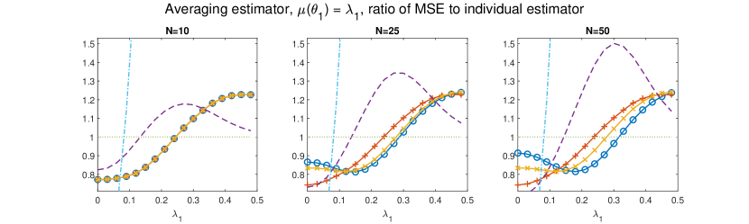
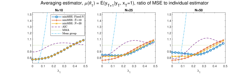
Figure 1: MSE performance of the unit averaging estimator relative to the individual estimator. The focus parameters are the autoregressive parameter $\lambda_{1}$ and conditional mean (forecast). $T=60$, $N=10,25,50$

Figure 1 summarizes the main results of the simulation study based on 2500 replications. We report performance of different averaging strategies in terms of MSE relative to the individual estimator for a range of values of $\lambda_{1}$. As the distribution of $\lambda_{1}$ is symmetric, we report performance for half of the support of $\lambda_{1}$. In each plot, we plot the MSE of different averaging estimators relative to the MSE of the individual estimator of unit 1. A value larger than 1 indicates that the individual estimator is more efficient. The minimum MSE unit averaging estimator performs favorably throughout most of the parameter space. Large-$N$ approximations work better for $\lambda_{1}$ closer to $\operatorname{\mathbb{E}}(\lambda_{1})=0$. However, for larger values of $\lambda_{1}$ the flexibility of the fixed-$N$ regime is an advantage, as it can freely choose units most similar to unit 1. None of the averaging estimators dominate the other. As expected, the mean group estimator performs very well close to the mean of $\lambda_{1}$, but bias starts to dominate as $\lambda_{1}$ is increased. AIC weights offers a risk profile somewhat similar to that of the MG estimator for values closer mean of $\lambda_{1}$. As $\lambda_{1}$ becomes larger, AIC moves towards the individual estimator. As noted above, MMA is effectively minimal BIC model selection in the context of unit averaging. MMA almost always selects unit 1, and correspondingly MMA does not offer improvements over the individual estimator.

5 Empirical Application

We illustrate our methodology with a pseudo-real time nowcasting exercise for quarterly GDP for a panel of European countries. GDP prediction is a natural application of our unit averaging methodology. There is evidence of considerable heterogeneity between countries, yet at the same time pooling the data at least partially improves prediction accuracy (Garcia-Ferrer et al., 1987; Hoogstrate et al., 2000; Marcellino et al., 2003). The design of our application follows standard practices in the nowcasting literature (Marcellino and Schumacher, 2010; Schumacher, 2016). The literature on nowcasting is vast and we do not to cover it here. We refer to Bańbura et al. (2013) for a survey.

We use quarterly GDP data from 1995Q1 to 2019Q4 for 12 European countries: the 11 founding Eurozone economies and the UK. We enrich our dataset with a set of 162 monthly GDP predictors for each country. The set of predictors include both real, price, and survey data. Table OA.1 in the online appendix contains the complete list of variables and descriptions. All non-survey data is available from Eurostat whereas the survey data is available from the DG ECFIN. We use final data releases incorporating all revisions, making our study a pseudo-real time one.

Our empirical design takes into account both the delays in publication of monthly data (“ragged-edge problem”) and the impact of timing on the information set available (“vintages” of data). First, the predictor variables are typically released with different delays after the end of the corresponding month, which is known as the “ragged-edge” problem (Wallis, 1986). We adopt a stylized release calendar of bimonthly releases to account for this (table OA.1 in the online appendix lists the release delay for all variables). Second, as the quarter goes by, more data becomes available. Each possible position in time determines a data “vintage”. We assume that a month has 4 weeks; in accordance with our release calendar, we nowcast every two weeks starting from the first day of the quarter at $-12$ weeks (relative to the quarter end) until $+4$ weeks after the end of the quarter (GDP is released at +6 weeks). Formally, let $t$ index months. Then $v=-3,-5/2,-2,\ldots,1/2,+1$ is a fractional value that describes the monthly position (or vintage) relative to the end of the quarter, in increments of two weeks.

We nowcast GDP in quarter $3t$ using all information available at time $3t+v$, separately for each value of $v\in\{-3,-5/2,\dots,+1\}$. As we have a large number of predictors available at monthly frequency, we opt for factor unrestricted MIDAS (U-MIDAS) (Foroni et al., 2015). Given $v$, for each country we estimate monthly factors $f_{i\,t}$ with $\hat{f}_{i\,t|v}$ for all $t=1,\dots,\lfloor T+v\rfloor$ using the full dataset available at $T+v$. The GDP is modeled as

$$y_{i\,3t}=\alpha_{i|v}+\sum_{k=0}^{11}\beta_{i\,k|v}\hat{f}_{i\,\lfloor 3t+v-k\rfloor|v}+\lambda_{i|v}y_{i\,3(t-1)}+\varepsilon_{i\,3t|v},$$

where $y_{i\,3t}$ is GDP of country $i$ in quarter $3t$ and $\varepsilon_{i\,3t|v}$ is the prediction error. The country factors estimates $\hat{f}_{i\,t|v}$ are extracted from the large set of predictor variables using the EM-PCA method (Stock and Watson, 1999). If GDP of quarter $3(t-1)$ is not available at moment $v$, we use $y_{i\,3(t-2)}$ instead. We use only one factor for prediction following Marcellino and Schumacher (2010) and we include the lag of GDP following Clements and Galvão (2008). We nowcast GDP for each country using the conditional mean of GDP implied by the U-MIDAS specification. Parameter estimation is carried out using a rolling-windows of sizes 44, 60 and 76 quarters. Factors are also re-estimated every two weeks using the all the data available at each point in time.

We estimate the conditional mean using the fixed-$N$ minimum MSE unit averaging estimator, since cross-sectional dimension is not large and each unit is potentially relevant. The performance of our minimum MSE unit averaging estimator is benchmarked against the individual, mean group, and averaging estimators using AIC and Mallows weights.

In table 1 we provide a summary of forecasting performance results for GDP nowcasting. The table reports the MSE of the individual estimator as well as the MSE relative to the individual estimator for all other strategies. The table reports results for the five largest economies in our sample along with the GDP-weighted mean. We select the vintages that correspond to $-6,0,+4$ weeks relative to the end of the quarter (corresponding to $v=-3/2,0,+1$). Full results for all vintages and countries are provided in table OA.7 in the online appendix, and they are similar to the ones reported here.

		$-6$ weeks			$0$ weeks			$+4$ weeks
	Averaging	44q	60q	76q	44q	60q	76q	44q	60q	76q
Mean	Individual	1.113	0.986	1.167	0.973	1.010	1.196	0.933	0.914	1.124
	minMSE	0.916	0.936	0.907	0.889	0.936	0.910	0.881	0.928	0.901
	AIC	0.933	0.962	0.980	0.908	0.960	0.974	0.878	0.949	0.955
	MMA	1.119	1.178	1.099	1.011	1.036	1.114	1.000	0.921	0.916
	Mean group	1.417	1.570	1.524	1.635	1.696	1.505	1.879	1.704	1.489
DE	Individual	0.661	0.546	0.537	0.509	0.421	0.434	0.565	0.449	0.456
	minMSE	0.793∗	0.822	0.815	0.787∗	0.818	0.775	0.821∗	0.809	0.794
	AIC	0.963∗	0.977∗	0.989	0.974	0.982∗	0.973	0.978	0.989∗	0.978
	MMA	1.002	1.257	1.098	0.860	0.970	0.742	0.741	0.830	0.834
	Mean group	0.987	0.937	0.773	1.069	1.157	0.742	0.957	1.153	0.849
FR	Individual	0.194	0.154	0.129	0.143	0.100	0.086	0.155	0.121	0.098
	minMSE	0.988	1.067	1.037	0.971	1.059	1.159	0.916	0.978	1.069
	AIC	0.883∗	0.934	0.975	0.833∗	0.978	1.049	0.828∗	0.935∗	0.999
	MMA	1.223	1.343∗	1.139	1.082	1.372∗	1.659∗	1.164	1.048	1.337
	Mean group	2.125∗	2.068∗	1.348	2.736∗	2.942∗	2.169∗	2.473∗	2.652∗	2.156∗
IT	Individual	0.591	0.253	0.156	0.279	0.178	0.116	0.232	0.131	0.082
	minMSE	0.893∗	0.908∗	0.852∗	0.973	0.974	0.858∗	1.046	1.025	0.857∗
	AIC	0.945	0.972∗	0.980	0.955	0.951∗	0.976∗	0.947	0.969∗	0.975∗
	MMA	0.907	0.710∗	0.729∗	1.323	0.650∗	0.704	1.351	0.917	0.688∗
	Mean group	0.895	0.901	0.822	1.289	1.042	0.719	1.491∗	1.595∗	1.239
ES	Individual	0.288	0.198	0.147	0.233	0.121	0.106	0.253	0.114	0.102
	minMSE	0.919	0.909∗	0.856∗	0.955	0.951	0.927	0.957	0.919	0.889
	AIC	0.958	0.961∗	0.974∗	0.860	0.940	0.940∗	0.813∗	0.934	0.933∗
	MMA	0.928	0.900	1.000	0.922	0.906	1.002	1.312	0.821	1.000
	Mean group	1.237∗	1.427∗	1.225	1.011	1.561∗	1.352	0.946	1.886∗	1.248
UK	Individual	0.281	0.116	0.044	0.254	0.142	0.047	0.244	0.142	0.047
	minMSE	0.928	0.988	0.953	0.840	0.984	0.868	0.743	1.034	0.913
	AIC	0.871∗	0.933	0.953	0.876	0.958	0.941	0.726∗	0.917∗	0.898∗
	MMA	1.457	1.375∗	1.350	1.240	1.318∗	1.580	1.523	1.069	0.854
	Mean group	1.714	2.444∗	3.688∗	2.530∗	2.445∗	3.121∗	4.330∗	2.214∗	2.650∗

Table 1: Nowcasting MSE. For individual estimator: absolute value. For averaging estimators: MSE relative to individual estimator. For different estimation window sizes (44, 60, 76); selected weekly horizons relative to quarter end ($-6,0,+4$ weeks). * – forecasting performance difference significant at 10% in Diebold-Mariano test (Diebold and Mariano, 1995)

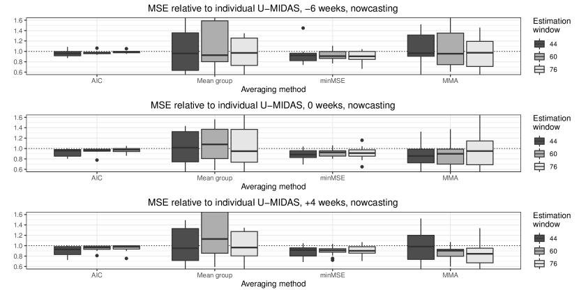
Figure 2: Distribution of relative MSEs across countries. Split by different averaging strategies and estimation window size. Same weekly positions as reported in table 1

Our key finding is that averaging with smooth data-dependent criteria – minimum MSE or AIC weights – generally leads to improved forecasting performance, though the degree of improvement varies with the country in question. This is clear from table 1, as the vast majority of entries corresponding to those weights display relative MSE smaller than one, with improvements reaching up to 20%. The average gain in performance is on the scale of about 9% for minimum MSE weights and 5% for AIC weights. We also observe that minimum MSE weights and AIC weights do not uniformly dominate each other.

Figure 2 provides a box plot for relative MSEs for nowcasting GDP for all the countries in the panel for the vintages considered in table 1. The figure illustrates that the favorable performance is robust across countries and not limited to the five biggest economies reported in table 1. Both minimum MSE and AIC weights generally lead to an improvement in performance, as both rarely have relative MSE above one. There is some evidence that the minimum MSE weights have a greater upside, at the price of potentially some more variability in the results, while AIC leads to smaller, but more tightly concentrated improvements. Further, we find that averaging is more attractive for the smallest sample size of $T=44$, with relative MSE generally approaching one as $T$ increases. This can be clearly seen in figure 2, as the improvement range for AIC and minimum MSE weights becomes more concentrated and to closer to one. As previously remarked, as $T$ increases, the minimum MSE estimator converges to the individual estimator; a similar point applies to AIC weights if the log likelihood is not divided by samples size and allowed to diverge as sample size grows.

Averaging methods that are data-independent (mean group) or not smooth (MMA) lead to generally poor results. While capable of offering improvements, the two approaches often lead to significantly worse performance than the individual estimator, regardless of $T$. This is clear from figure 2, where the distribution of the MSE of both averaging strategies has substantial mass above one.

We remark that the online appendix contains a number of additional robustness checks. First, we consider nowcasting using bridge equations instead of U-MIDAS. Second, we consider one- and two-quarter-ahead GDP forecasting. The evidence emerging from these additional robustness checks on the performance of minimum MSE unit averaging estimator is consistent with the overall evidence reported here.

6 Conclusions

In this work we introduce a unit averaging estimator to recover unit-specific parameters in a general class of panel data models with heterogeneous parameters. The procedure consists in estimating the parameter of a given unit using a weighted average of all the unit-specific parameter estimators in the panel. The weights of the average are determined by minimizing an MSE criterion. The paper studies the properties of the procedures using a local heterogeneity framework that builds upon the literature on frequentist model averaging (Hjort and Claeskens, 2003; Hansen, 2008). An application to GDP nowcasting for a panel of European countries shows that the procedure performs favorably for prediction relative to a number of alternative procedures.

Proofs of Results in the Main Text

Under assumption 1 we work conditional on $\{\bm{\eta}_{1},\bm{\eta}_{2},\dots\}$. We use $\operatorname{\mathbb{E}}[\cdot]$ to denote the expectation operator conditional on $\{\bm{\eta}_{1},\bm{\eta}_{2},\dots\}$, whereas $\operatorname{\mathbb{E}}_{\bm{\eta}}[\cdot]$ is the expectation taken with respect the distribution of $\bm{\eta}$. All results are shown to hold with probability one with respect to the distribution of $\bm{\eta}$ (denoted $\bm{\eta}$-a.s.).

A.1 Proof of Lemma 1

Recall that the data vector $\bm{z}_{i\,t}$ takes values in $\mathcal{Z}\subset\operatorname{\mathbb{R}}^{d}$ and define the data matrix $\bm{z}_{i}=(\bm{z}_{i\,1}^{\prime},\ldots,\bm{z}_{i\,T}^{\prime})^{\prime}$ that takes values in $\mathcal{Z}^{T}=\prod_{t=1}^{T}\mathcal{Z}$. Recall that that the parameter vector $\bm{\theta}=(\theta_{1},\dots,\theta_{p})$ takes values in $\Theta\subset\mathbb{R}^{p}$. We denote by $\nabla m(\bm{\theta},\bm{z}_{i\,t})$ the gradient vector of $m$ with respect to $\bm{\theta}$, by $\nabla^{2}m(\bm{\theta},\bm{z}_{i\,t})$ the Hessian matrix of $m$ with respect to $\bm{\theta}$, by $\nabla_{\theta_{k}}m(\bm{\theta},\bm{z}_{i\,t})$ the partial derivative of $m$ with respect to $\theta_{k}$, and by $\nabla^{2}_{\bm{\theta}\,\theta_{k}}$ the gradient vector of $\nabla_{\theta_{k}}m(\bm{\theta},\bm{z}_{i\,t})$ with respect to $\bm{\theta}$.

We establish a mean value theorem that does not require compactness of $\Theta$.

Lemma A.1.1.

Suppose assumption 3 is satisfied. Then for each unit $i$, any $T$ and any $k=1,\ldots,p$ there exists a measurable function $\tilde{\bm{\theta}}_{i\,k}$ from $\mathcal{Z}^{T}$ to $\Theta$ such that the individual estimator $\hat{\bm{\theta}}_{i}$ of eq. (2) satisfies

$$\dfrac{1}{T}\sum_{t=1}^{T}\nabla_{\theta_{k}}m(\hat{\bm{\theta}}_{i},\bm{z}_{i\,t})=\dfrac{1}{T}\sum_{t=1}^{T}\nabla_{\theta_{k}}m({\bm{\theta}}_{i},\bm{z}_{i\,t})$$ (A.1.1)

$$\quad+\left[\dfrac{1}{T}\sum_{t=1}^{T}\nabla^{2}_{\bm{\theta}\,\theta_{k}}m(\tilde{\bm{\theta}}_{i\,k},\bm{z}_{i\,t})\right]^{\prime}\left(\hat{\bm{\theta}}_{i}-\bm{\theta}_{i}\right)~{},$$ (A.1.2)

where $\tilde{\bm{\theta}}_{i\,k}$ lies on the segment joining $\hat{\bm{\theta}}_{i}$ and $\bm{\theta}_{i}$.

Further, suppose 5 is satisfied. Then for each $i$ and any $T$ there exist measurable functions $\bar{\bm{\theta}}_{i}$, $\acute{\bm{\theta}}_{i}$ and $\check{\bm{\theta}}_{i}$ from $\mathcal{Z}^{T}$ to $\Theta$ such that the individual estimator $\hat{\bm{\theta}}_{i}$ of eq. (2) satisfies

$$\mu(\hat{\bm{\theta}}_{i}) =\mu(\bm{\theta}_{1})+\nabla\mu(\bar{\bm{\theta}}_{i})^{\prime}(\hat{\bm{\theta}}_{i}-\bm{\theta}_{1})~{},$$ (A.1.3)

$$\mu(\hat{\bm{\theta}}_{i}) =\mu(\bm{\theta}_{1})+\bm{d}^{\prime}_{1}(\hat{\bm{\theta}}_{i}-\bm{\theta}_{1})+\dfrac{1}{2}(\hat{\bm{\theta}}_{i}-\bm{\theta}_{1})^{\prime}\nabla^{2}\mu(\acute{\bm{\theta}}_{i})(\hat{\bm{\theta}}_{i}-\bm{\theta}_{1})~{},$$ (A.1.4)

$$\mu(\hat{\bm{\theta}}_{i}) =\mu(\bm{\theta}_{i})+\bm{d}^{\prime}_{i}(\hat{\bm{\theta}}_{i}-\bm{\theta}_{i})+\dfrac{1}{2}(\hat{\bm{\theta}}_{i}-\bm{\theta}_{i})^{\prime}\nabla^{2}\mu(\check{\bm{\theta}}_{i})(\hat{\bm{\theta}}_{i}-\bm{\theta}_{i})~{},$$ (A.1.5)

where $\bm{d}_{1}=\nabla\mu(\bm{\theta}_{1})$; $\bar{\bm{\theta}}_{i}$ and $\acute{\bm{\theta}}_{i}$ lie on the segment joining $\hat{\bm{\theta}}_{i}$ and $\bm{\theta}_{1}$; and $\check{\bm{\theta}}_{i}$ lies on the segment joining $\hat{\bm{\theta}}_{i}$ and $\bm{\theta}_{i}$.

Proof.

Fix $k\in\{1,\dots,p\}$ and define the function $f_{i}:\mathcal{Z}^{T}\times[0,1]\to\operatorname{\mathbb{R}}$ as

$$f_{i}(\bm{z}_{i},y) =\dfrac{1}{T}\sum_{t=1}^{T}\nabla_{\theta_{k}}m(\hat{\bm{\theta}}_{i},\bm{z}_{i\,t})-\dfrac{1}{T}\sum_{t=1}^{T}\nabla_{\theta_{k}}m({\bm{\theta}}_{i},\bm{z}_{i\,t})$$ (A.1.6)

$$\quad-\left[\dfrac{1}{T}\sum_{t=1}^{T}\nabla^{2}_{\bm{\theta}\,\theta_{k}}m(y\hat{\bm{\theta}}_{i}+(1-y)\bm{\theta}_{i},\bm{z}_{i})\right]^{\prime}(\hat{\bm{\theta}}_{i}-\bm{\theta}_{i})~{}.$$ (A.1.7)

3 implies that $f_{i}$ is well-defined, as for each $y\in[0,1]$ we have that $y\hat{\bm{\theta}}_{i}+(1-y)\bm{\theta}_{i}\in\Theta$. $f_{i}$ is a measurable function of $\bm{z}_{i}$ for every fixed value $y\in[0,1]$, as $\hat{\bm{\theta}}_{i}$ and $m$ are measurable functions of $\bm{z}_{i}$ and $m$ is continuously differentiable in $\bm{\theta}$. $f_{i}$ is a continuous function of $y$ for every value of $\bm{z}_{i}$.

Define the correspondence $\varphi_{i}:\mathcal{Z}^{T}\to[0,1]$ as $\varphi_{i}(\bm{z}_{i})=\left\{y\in[0,1]:f_{i}(\bm{z}_{i},y)=0\right\}$. The function $f_{i}$ satisfies the assumptions of corollary 18.8 in Aliprantis and Border (2006), and so $\varphi_{i}$ is a measurable correspondence. $\varphi_{i}(\bm{z}_{i})$ is nonempty for every $\bm{z}_{i}$, as by the mean value theorem, for every fixed value of $\bm{z}_{i}$ there exists some $\tilde{y}\in[0,1]$ such that

$$\dfrac{1}{T}\sum_{t=1}^{T}\nabla_{\theta_{k}}m(\hat{\bm{\theta}}_{i},\bm{z}_{i\,t}) =\dfrac{1}{T}\sum_{t=1}^{T}\nabla_{\theta_{k}}m({\bm{\theta}}_{i},\bm{z}_{i\,t})$$ (A.1.8)

$$\quad+\left[\dfrac{1}{T}\sum_{t=1}^{T}\nabla^{2}_{\bm{\theta},\theta_{k}}m(\tilde{y}\hat{\bm{\theta}}_{i}+(1-\tilde{y})\bm{\theta}_{i},\bm{z}_{i\,t})\right]^{\prime}\left(\hat{\bm{\theta}}_{i}-\bm{\theta}_{i}\right).$$ (A.1.9)

In addition, $\varphi_{i}(\bm{z}_{i})$ is closed for every $\bm{z}_{i}$ as $m$ is twice continuously differentiable in $\bm{\theta}$ by assumption 3. Then by the Kuratowski-Ryll-Nardzewski measurable selection theorem (theorem 18.13 in Aliprantis and Border (2006)), $\varphi_{i}(\bm{z}_{i})$ admits a measurable selector $\tilde{y}_{i\,k}=\tilde{y}_{i\,k}(\bm{z}_{i})$. Finally, define $\tilde{\bm{\theta}}_{i\,k}=\tilde{y}_{i\,k}\hat{\bm{\theta}}_{i}+(1-\tilde{y}_{i\,k})\bm{\theta}_{i}$ and note that $\tilde{\bm{\theta}}_{i\,k}$ satisfies the requirements of the lemma. This establishes the first claim of the lemma.

The proof of the second claim of the lemma is analogous. ∎

The following lemma is needed to prove lemmas 1 and A.2.1.

Lemma A.1.2.

Suppose 3 is satisfied. Let $\tilde{\bm{\theta}}_{i\,j}:\mathcal{Z}^{T}\rightarrow\mathbb{R}^{p}$ for $j=1,\dots,p$ be a sequence of measurable functions that lie on the segment joining $\bm{\theta}_{i}$ and $\hat{\bm{\theta}}_{i}$ and define

$$\hat{\bm{H}}_{i\,T}=\begin{bmatrix}\left[\dfrac{1}{T}\sum_{t=1}^{T}\nabla^{2}_{\bm{\theta},\theta_{1}}m(\tilde{\bm{\theta}}_{i\,1},\bm{z}_{i\,t})\right]^{\prime}\\ \cdots\\ \left[\dfrac{1}{T}\sum_{t=1}^{T}\nabla^{2}_{\bm{\theta},\theta_{p}}m(\tilde{\bm{\theta}}_{i\,p},\bm{z}_{i\,t})\right]^{\prime}\end{bmatrix}.$$ (A.1.10)

Then for all $T>T_{0}$ the matrix $\hat{\bm{H}}_{i\,T}$ (i) is a.s. nonsingular and (ii) satisfies

$$\operatorname{\mathbb{E}}\left[\left\lVert\bm{H}_{i}^{-1}-\hat{\bm{H}}_{i\,T}^{-1}\right\rVert_{\infty}^{\frac{2(2+\delta)(1+\delta)}{\delta}}\right]\leq p^{\frac{(2+\delta)(1+\delta)}{\delta}}\underline{\lambda}_{\bm{H}}^{-\frac{2(2+\delta)(1+\delta)}{\delta}}C_{\nabla^{2}m}~{},$$ (A.1.11)

where $\bm{H}_{i}=\lim_{T\to\infty}\operatorname{\mathbb{E}}\left[T^{-1}\sum_{t=1}^{T}\nabla^{2}m(\bm{\theta}_{i},\bm{z}_{i\,t})\right]$.

Proof.

The proof of assertion $(i)$ is based on showing that $\left\lVert(\bm{H}_{i}-\hat{\bm{H}}_{i\,T})\bm{H}_{i}^{-1}\right\rVert_{\infty}<1$ holds almost surely, which implies that the matrix $\hat{\bm{H}}_{i\,T}$ is a.s. nonsingular. Let $\bm{H}_{i}^{-1}=(h^{ij})$ and observe that

$$\hat{\bm{H}}_{i\,T}\bm{H}_{i}^{-1}=\begin{bmatrix}\sum_{k=1}^{p}\nabla^{2}_{\theta_{k}\,\theta_{1}}m(\tilde{\bm{\theta}}_{i\,1},\bm{z}_{i\,t})h^{k1}&\cdots&\sum_{k=1}^{p}\nabla^{2}_{\theta_{k}\,\theta_{1}}m(\tilde{\bm{\theta}}_{i\,1},\bm{z}_{i\,t})h^{kp}\\ \sum_{k=1}^{p}\nabla^{2}_{\theta_{k}\,\theta_{2}}m(\tilde{\bm{\theta}}_{i\,2},\bm{z}_{i\,t})h^{k1}&\cdots&\sum_{k=1}^{p}\nabla^{2}_{\theta_{k}\,\theta_{2}}m(\tilde{\bm{\theta}}_{i\,2},\bm{z}_{i\,t})h^{kp}\\ \vdots&\ddots&\vdots\\ \sum_{k=1}^{p}\nabla^{2}_{\theta_{k}\,\theta_{p}}m(\tilde{\bm{\theta}}_{i\,p},\bm{z}_{i\,t})h^{k1}&\cdots&\sum_{k=1}^{p}\nabla^{2}_{\theta_{k}\,\theta_{p}}m(\tilde{\bm{\theta}}_{i\,p},\bm{z}_{i\,t})h^{kp}\end{bmatrix}~{}.$$ (A.1.12)

Row $j$ of $\hat{\bm{H}}_{i\,T}\bm{H}_{i}^{-1}-\bm{I}$ coincides with row $j$ of $\left(T^{-1}\sum_{t=1}^{T}\nabla^{2}m\left(\tilde{\bm{\theta}}_{i\,j},\bm{z}_{i\,t}\right)\right)\bm{H}^{-1}-\bm{I}$. Then we have that

$$\left\lVert(\bm{H}_{i}-\hat{\bm{H}}_{i\,T})\bm{H}_{i}^{-1}\right\rVert_{\infty} =\left\lVert\hat{\bm{H}}_{i\,T}\bm{H}_{i}^{-1}-\bm{I}\right\rVert_{\infty}$$ (A.1.13)

$$\leq\max_{1\leq j\leq p}\left\lVert\left(T^{-1}\sum_{t=1}^{T}\nabla^{2}m(\tilde{\bm{\theta}}_{i\,j},\bm{z}_{i\,t})\right)\bm{H}^{-1}_{i}-\bm{I}\right\rVert_{\infty}$$ (A.1.14)

$$\leq\sup_{\bm{\theta}\in[\bm{\theta}_{i},\hat{\bm{\theta}}_{i}]}\left\lVert\left(T^{-1}\sum_{t=1}^{T}\nabla^{2}m({\bm{\theta}},\bm{z}_{i\,t})\right)\bm{H}^{-1}_{i}-\bm{I}\right\rVert_{\infty}$$ (A.1.15)

$$\equiv D_{i\,T}~{},$$ (A.1.16)

where the second inequality holds as all $\tilde{\bm{\theta}}_{i\,j}$ lie on the segment joining $\bm{\theta}_{i}$ and $\hat{\bm{\theta}}_{i}$ and where $D_{i\,T}$ is defined in 3. 3 implies $D_{i\,T}<1$ a.s. for $T>T_{0}$, and thus $\left\lVert(\bm{H}_{i}-\hat{\bm{H}}_{i\,T})\bm{H}_{i}^{-1}\right\rVert_{\infty}<1$ a.s. for $T>T_{0}$, which implies the first claim.
As $\hat{\bm{H}}_{i\,T}$ is invertible for $T>T_{0}$ we have (Horn and Johnson, 2012, section 5.8)

$$\left\lVert\bm{H}_{i}^{-1}-\hat{\bm{H}}_{i\,T}^{-1}\right\rVert_{\infty}\leq\left\lVert\bm{H}_{i}^{-1}\right\rVert_{\infty}\dfrac{\left\lVert\bm{H}^{-1}_{i}\hat{\bm{H}}_{i\,T}-\bm{I}\right\rVert_{\infty}}{1-\left\lVert\bm{H}^{-1}_{i}\hat{\bm{H}}_{i\,T}-\bm{I}\right\rVert_{\infty}}\leq\left\lVert\bm{H}_{i}^{-1}\right\rVert_{\infty}\dfrac{D_{i\,T}}{1-D_{i\,T}}~{},$$ (A.1.17)

where the last inequality follows from (A.1.16). Taking expectations, we obtain that

$$\operatorname{\mathbb{E}}\left[\left\lVert\bm{H}_{i}^{-1}-\hat{\bm{H}}_{i}^{-1}\right\rVert_{\infty}^{\frac{2(2+\delta)(1+\delta)}{\delta}}\right] \leq\left\lVert\bm{H}_{i}^{-1}\right\rVert^{\frac{2(2+\delta)(1+\delta)}{\delta}}_{{\infty}}\operatorname{\mathbb{E}}\left[\left(\dfrac{D_{i\,T}}{1-D_{i\,T}}\right)^{\frac{2(2+\delta)(1+\delta)}{\delta}}\right]$$ (A.1.18)

$$\leq p^{\frac{(2+\delta)(1+\delta)}{\delta}}\left\lVert\bm{H}_{i}^{-1}\right\rVert^{\frac{2(2+\delta)(1+\delta)}{\delta}}C_{\nabla^{2}m}$$ (A.1.19)

$$\leq p^{\frac{(2+\delta)(1+\delta)}{\delta}}\underline{\lambda}_{\bm{H}}^{-\frac{2(2+\delta)(1+\delta)}{\delta}}C_{\nabla^{2}m}~{},$$ (A.1.20)

which establishes the second claim. ∎

Proof of lemma 1.

3 and Lemma A.1.1 imply that

$$0 =\dfrac{1}{T}\sum_{t=1}^{T}\nabla_{\theta_{k}}m(\hat{\bm{\theta}}_{i},\bm{z}_{i\,t})$$ (A.1.21)

$$=\dfrac{1}{T}\sum_{t=1}^{T}\nabla_{\theta_{k}}m({\bm{\theta}}_{i},\bm{z}_{i\,t})+\left[\dfrac{1}{T}\sum_{t=1}^{T}\nabla^{2}_{\bm{\theta},\theta_{k}}m(\tilde{\bm{\theta}}_{i\,k},\bm{z}_{i\,t})\right]^{\prime}\left(\hat{\bm{\theta}}_{i}-\bm{\theta}_{i}\right)~{},$$ (A.1.22)

where $\tilde{\bm{\theta}}_{i\,k}$ lies on the segment joining $\bm{\theta}_{i}$ and $\hat{\bm{\theta}}_{i}$. Define the matrix

$$\hat{\bm{H}}_{i\,T}=\begin{bmatrix}\left[\dfrac{1}{T}\sum_{t=1}^{T}\nabla^{2}_{\bm{\theta},\theta_{1}}m(\tilde{\bm{\theta}}_{i\,1},\bm{z}_{i\,t})\right]^{\prime}\\ \cdots\\ \left[\dfrac{1}{T}\sum_{t=1}^{T}\nabla^{2}_{\bm{\theta},\theta_{p}}m(\tilde{\bm{\theta}}_{i\,p},\bm{z}_{i\,t})\right]^{\prime}\end{bmatrix}.$$ (A.1.23)

As all $\hat{\bm{\theta}}_{i\,k}$ lie between $\bm{\theta}_{i}$ and $\hat{\bm{\theta}}_{i}$, by lemma A.1.2 the matrix $\hat{\bm{H}}_{i\,T}$ is a.s. nonsingular for $T>T_{0}$. Observe that $\hat{\bm{\theta}}_{i}-\bm{\theta}_{i}=(\hat{\bm{\theta}}_{i}-\bm{\theta}_{1})-(\bm{\theta}_{i}-\bm{\theta}_{1})$. Combining the above two observations, we obtain that for $T>T_{0}$ it holds that

$$\sqrt{T}\left(\hat{\bm{\theta}}_{i}-\bm{\theta}_{1}\right)=-\hat{\bm{H}}_{i\,T}^{-1}\dfrac{1}{\sqrt{T}}\sum_{t=1}^{T}\nabla m({\bm{\theta}}_{i},\bm{z}_{i\,t})+(\bm{\eta}_{i}-\bm{\eta}_{1}).$$ (A.1.24)

By assumption 3 and lemma A.1.2, it holds that

$$-\hat{\bm{H}}_{i\,T}^{-1}\dfrac{1}{\sqrt{T}}\sum_{t=1}^{T}\nabla m({\bm{\theta}}_{i},\bm{z}_{i\,t})\Rightarrow N(0,\bm{V}_{i}).$$ (A.1.25)

The convergence is joint as all units are independent by 2.
The second assertion follows from the delta method and the observation that $\nabla\mu(\bm{\theta}_{1})=\nabla\mu(\bm{\theta}_{0}+T^{-1/2}\bm{\eta}_{1})\to\nabla\mu(\bm{\theta}_{0})=\bm{d}_{0}$ under the continuity assumption of 5. ∎

A.2 Proof of Theorem 3.1

Before presenting the proof of theorem 3.1 we introduce a number of intermediate results.

Lemma A.2.1.

Suppose 1 and 3 are satisfied. Let $\delta$ be as in 3. Then there exist finite constants $C_{\hat{\bm{\theta}},1},C_{\hat{\bm{\theta}},1+\delta/2},C_{\hat{\bm{\theta}},2},C_{\hat{\bm{\theta}},2+\delta}$, which do not depend on $i$ or $T$, such that the following moment bounds hold for the individual estimator (2) for all $T>T_{0}$

$$\operatorname{\mathbb{E}}\left[\left\lVert\sqrt{T}(\hat{\bm{\theta}}_{i}-\bm{\theta}_{i})\right\rVert^{k}\right] \leq C_{\hat{\bm{\theta}},k}~{},\quad k=1,1+\delta/2,2,2+\delta,$$ (A.2.1)

$$\operatorname{\mathbb{E}}\left[\left\lVert\sqrt{T}(\hat{\bm{\theta}}_{i}-\bm{\theta}_{1})\right\rVert^{2}\right] \leq C_{\hat{\bm{\theta}},2}+2C_{\hat{\bm{\theta}},1}\left\lVert\bm{\eta}_{i}-\bm{\eta}_{1}\right\rVert+\left\lVert\bm{\eta}_{i}-\bm{\eta}_{1}\right\rVert^{2}~{}.$$ (A.2.2)

Proof.

Let the matrix $\hat{\bm{H}}_{i\,T}$ be defined as in eq. (A.1.23). By lemma A.1.2 the matrix $\hat{\bm{H}}_{i\,T}$ is non-singular for $T>T_{0}$. Then, as in the proof of lemma 1, for $T>T_{0}$ it holds that

$$\sqrt{T}\left(\hat{\bm{\theta}}_{i}-\bm{\theta}_{i}\right) =-\hat{\bm{H}}^{-1}_{i\,T}\dfrac{1}{\sqrt{T}}\sum_{t=1}^{T}\nabla m({\bm{\theta}}_{i},\bm{z}_{i\,t})$$ (A.2.3)

$$=-\bm{H}_{i}^{-1}\dfrac{1}{\sqrt{T}}\sum_{t=1}^{T}\nabla m({\bm{\theta}}_{i},\bm{z}_{i\,t})+\left(\bm{H}_{i}^{-1}-\hat{\bm{H}}_{i\,T}^{-1}\right)\dfrac{1}{\sqrt{T}}\sum_{t=1}^{T}\nabla m({\bm{\theta}}_{i},\bm{z}_{i\,t})~{},$$ (A.2.4)

where $\bm{H}_{i}=\lim_{T\to\infty}\operatorname{\mathbb{E}}\left(\nabla^{2}T^{-1}\sum_{t=1}^{T}m(\bm{\theta}_{i},\bm{z}_{i\,t})\right)$. We separately bound the $(2+\delta)$-th moment of the norm for the two terms above. For the first term we have

$$\operatorname{\mathbb{E}}\left[\left\lVert\bm{H}_{i}^{-1}\dfrac{1}{\sqrt{T}}\sum_{t=1}^{T}\nabla m({\bm{\theta}}_{i},\bm{z}_{i\,t})\right\rVert^{2+\delta}\right]$$ (A.2.5)

$$\leq\operatorname{\mathbb{E}}\left[\left\lVert\bm{H}_{i}^{-1}\right\rVert^{2+\delta}\left\lVert\dfrac{1}{\sqrt{T}}\sum_{t=1}^{T}\nabla m({\bm{\theta}}_{i},\bm{z}_{i\,t})\right\rVert^{2+\delta}\right]$$ (A.2.6)

$$\leq\left\lVert\bm{H}_{i}^{-1}\right\rVert^{2+\delta}\operatorname{\mathbb{E}}\left[\left\lVert\dfrac{1}{\sqrt{T}}\sum_{t=1}^{T}\nabla m({\bm{\theta}}_{i},\bm{z}_{i\,t})\right\rVert^{2+\delta}\right]$$ (A.2.7)

$$\leq\underline{\lambda}_{\bm{H}}^{-2-\delta}C_{\nabla m}^{\frac{2+\delta}{2(1+\delta)}},$$ (A.2.8)

where the first inequality follows from $\left\lVert Ax\right\rVert\leq\left\lVert A\right\rVert\left\lVert x\right\rVert$, and the last line follows by assumption 3 and by Jensen’s inequality.

For the second term we have

$$\operatorname{\mathbb{E}}\left[\left\lVert\left(\bm{H}_{i}^{-1}-\hat{\bm{H}}_{i\,T}^{-1}\right)\dfrac{1}{\sqrt{T}}\sum_{t=1}^{T}\nabla m({\bm{\theta}}_{i},\bm{z}_{i\,t})\right\rVert^{2+\delta}\right]$$

$$\leq p^{\frac{2+\delta}{2}}\operatorname{\mathbb{E}}\left[\left\lVert\left(\bm{H}_{i}^{-1}-\hat{\bm{H}}_{i\,T}^{-1}\right)\dfrac{1}{\sqrt{T}}\sum_{t=1}^{T}\nabla m({\bm{\theta}}_{i},\bm{z}_{i\,t})\right\rVert^{2+\delta}_{\infty}\right]$$

$$\leq p^{\frac{2+\delta}{2}}\operatorname{\mathbb{E}}\left[\left\lVert\bm{H}_{i}^{-1}-\hat{\bm{H}}_{i\,T}^{-1}\right\rVert_{\infty}^{2+\delta}\left\lVert\dfrac{1}{\sqrt{T}}\sum_{t=1}^{T}\nabla m({\bm{\theta}}_{i},\bm{z}_{i\,t})\right\rVert^{2+\delta}_{\infty}\right]$$

$$\leq p^{\frac{2+\delta}{2}}\left(\operatorname{\mathbb{E}}\left[\left\lVert\bm{H}_{i}^{-1}-\hat{\bm{H}}_{i\,T}^{-1}\right\rVert_{\infty}^{\frac{2(2+\delta)(1+\delta)}{\delta}}\right]\right)^{\frac{\delta}{2(1+\delta)}}\left(\operatorname{\mathbb{E}}\left[\left\lVert\frac{1}{\sqrt{T}}\sum_{t=1}^{T}\nabla m({\bm{\theta}}_{i},\bm{z}_{i\,t})\right\rVert^{2(1+\delta)}_{\infty}\right]\right)^{\frac{1+\delta/2}{1+\delta}}$$

$$\leq p^{\frac{2+\delta}{2}}\left(p^{\frac{(2+\delta)(1+\delta)}{\delta}}\underline{\lambda}_{\bm{H}}^{-\frac{2(2+\delta)(1+\delta)}{\delta}}C_{\nabla^{2}m}\right)^{\frac{\delta}{2(1+\delta)}}\left(\operatorname{\mathbb{E}}\left[\left\lVert\frac{1}{\sqrt{T}}\sum_{t=1}^{T}\nabla m({\bm{\theta}}_{i},\bm{z}_{i\,t})\right\rVert^{2(1+\delta)}\right]\right)^{\frac{1+\delta/2}{1+\delta}}$$

$$\leq p^{\frac{2+\delta}{2}}\left(p^{\frac{(2+\delta)(1+\delta)}{\delta}}\underline{\lambda}_{\bm{H}}^{-\frac{2(2+\delta)(1+\delta)}{\delta}}C_{\nabla^{2}m}\right)^{\frac{\delta}{2(1+\delta)}}C_{\nabla\mu}^{\frac{1+\delta/2}{1+\delta}},$$

where the second inequality follows from $\left\lVert Ax\right\rVert_{\infty}\leq\left\lVert A\right\rVert_{\infty}\left\lVert x\right\rVert_{\infty}$; the third inequality from Hölder’s inequality applied with $p={(1+\delta)}/{(1+\delta/2)}>1$; the fourth inequality from lemma A.1.2, and the last line follows by assumption 3. Finally, we conclude that

$$\operatorname{\mathbb{E}}\left[\left\lVert\sqrt{T}(\hat{\bm{\theta}}_{i}-\bm{\theta}_{i})\right\rVert^{2+\delta}\right]$$ (A.2.9)

$$\leq 2^{1+\delta}\left[\underline{\lambda}_{\bm{H}}^{-2-\delta}C_{\nabla m}^{\frac{2+\delta}{2(1+\delta)}}+p^{\frac{2+\delta}{2}}\left(p^{\frac{(2+\delta)(1+\delta)}{\delta}}\underline{\lambda}_{\bm{H}}^{-\frac{2(2+\delta)(1+\delta)}{\delta}}C_{\nabla^{2}m}\right)^{\frac{\delta}{2(1+\delta)}}C_{\nabla\mu}^{\frac{1+\delta/2}{1+\delta}}\right]$$ (A.2.10)

$$\equiv C_{\hat{\bm{\theta}},2+\delta}~{},$$ (A.2.11)

where we note that $C_{\hat{\bm{\theta}},2+\delta}$ does not depend on $i$ or $T$. By Jensen’s inequality we have

$$\operatorname{\mathbb{E}}\left[\left\lVert\sqrt{T}\left(\hat{\bm{\theta}}_{i}-\bm{\theta}_{i}\right)\right\rVert^{2}\right] \leq C_{\hat{\bm{\theta}},2+\delta}^{\frac{2}{2+\delta}}\equiv C_{\hat{\bm{\theta}},2},$$ (A.2.12)

$$\operatorname{\mathbb{E}}\left[\left\lVert\sqrt{T}\left(\hat{\bm{\theta}}_{i}-\bm{\theta}_{i}\right)\right\rVert^{1+\delta/2}\right] \leq C_{\hat{\bm{\theta}},2+\delta}^{\frac{1}{2}}\equiv C_{\hat{\bm{\theta}},1+\delta/2},$$ (A.2.13)

$$\operatorname{\mathbb{E}}\left[\left\lVert\sqrt{T}\left(\hat{\bm{\theta}}_{i}-\bm{\theta}_{i}\right)\right\rVert\right] \leq C_{\hat{\bm{\theta}},2+\delta}^{\frac{1}{2+\delta}}\equiv C_{\hat{\bm{\theta}},1}~{},$$ (A.2.14)

which establishes the first part of the claim.
Next we note that

$$\operatorname{\mathbb{E}}\left[\left\lVert\sqrt{T}(\hat{\bm{\theta}}_{i}-\bm{\theta}_{1})\right\rVert^{2}\right]={\operatorname{\mathbb{E}}\left[T(\hat{\bm{\theta}}_{i}-\bm{\theta}_{1})^{\prime}(\hat{\bm{\theta}}_{i}-\bm{\theta}_{1})\right]}$$ (A.2.15)

$$\leq\operatorname{\mathbb{E}}\left[\left\lVert\sqrt{T}(\hat{\bm{\theta}}_{i}-\bm{\theta}_{i})\right\rVert^{2}\right]+2\left\lvert\operatorname{\mathbb{E}}\left[T(\hat{\bm{\theta}}_{i}-\bm{\theta}_{i})^{\prime}(\bm{\theta}_{i}-\bm{\theta}_{1})\right]\right\rvert+T\left(\bm{\theta}_{i}-\bm{\theta}_{1}\right)^{\prime}\left(\bm{\theta}_{i}-\bm{\theta}_{1}\right)$$ (A.2.16)

$$\leq\operatorname{\mathbb{E}}\left[\left\lVert\sqrt{T}(\hat{\bm{\theta}}_{i}-\bm{\theta}_{i})\right\rVert^{2}\right]+2\left\lVert\bm{\eta}_{i}-\bm{\eta}_{1}\right\rVert\operatorname{\mathbb{E}}\left[\left\lVert\sqrt{T}(\hat{\bm{\theta}}_{i}-\bm{\theta}_{i})\right\rVert\right]+\left\lVert\bm{\eta}_{i}-\bm{\eta}_{1}\right\rVert^{2}$$ (A.2.17)

$$\leq C_{\hat{\bm{\theta}},2}+2C_{\hat{\bm{\theta}},1}\left\lVert\bm{\eta}_{i}-\bm{\eta}_{1}\right\rVert+\left\lVert\bm{\eta}_{i}-\bm{\eta}_{1}\right\rVert^{2}~{},$$ (A.2.18)

where in the first inequality we add and subtract $\bm{\theta}_{i}$ in both parentheses, in the third inequality we apply the Cauchy-Schwarz inequality to the cross term and observe that under 1 $\sqrt{T}(\bm{\theta}_{i}-\bm{\theta}_{1})=\bm{\eta}_{i}-\bm{\eta}_{1}$. This establishes the second part of the claim. ∎

Lemma A.2.2.

Suppose 3 and 5 are satisfied. Let $\delta$ be as in assumption 3. Then for all $i$ and $T>T_{0}$ it holds that

$$\operatorname{\mathbb{E}}\left[\left\lvert\mu(\hat{\bm{\theta}}_{i})\right\rvert^{2+\delta}\right] <\infty$$ (A.2.19)

$$\operatorname{\mathbb{E}}\left[\left\lvert\sqrt{T}(\mu(\hat{\bm{\theta}}_{i})-\mu(\bm{\theta}_{i}))\right\rvert^{2+\delta}\right] \leq C_{\nabla\mu}^{2+\delta}C_{\hat{\bm{\theta}},2+\delta}$$ (A.2.20)

Proof.

Equation (A.1.3) in lemma A.1.1 implies $\mu(\hat{\bm{\theta}}_{i})=\mu(\bm{\theta}_{i})+\bar{\bm{d}}_{i}^{\prime}(\hat{\bm{\theta}}_{i}-\bm{\theta}_{i})$, where $\bar{\bm{d}}_{i}=\nabla\mu\left(\bar{\bm{\theta}}_{i}\right)$ for $\bar{\bm{\theta}}_{i}$ on the segment joining $\bm{\theta}_{i}$ and $\hat{\bm{\theta}}_{i}$. Raising both sides to the power of $(2+\delta)$ and applying the $C_{r}$ inequality we obtain that

$$\left\lvert\mu(\hat{\bm{\theta}}_{i})\right\rvert^{2+\delta}\leq 2^{1+\delta}\left[\left\lvert\mu(\bm{\theta}_{i})\right\rvert^{2+\delta}+\left\lvert\bar{\bm{d}}_{i}^{\prime}(\hat{\bm{\theta}}_{i}-\bm{\theta}_{i})\right\rvert^{2+\delta}\right].$$ (A.2.21)

By assumption 5 and the Cauchy-Schwarz inequality it holds that $\left\lvert\bar{\bm{d}}_{i}^{\prime}(\hat{\bm{\theta}}_{i}-\bm{\theta}_{i})\right\rvert^{2+\delta}\leq\left\lVert\bar{\bm{d}}_{1}\right\rVert^{2+\delta}\left\lVert\hat{\bm{\theta}}_{i}-\bm{\theta}_{i}\right\rVert^{2+\delta}\leq C_{\nabla\mu}^{2+\delta}\left\lVert\hat{\bm{\theta}}_{i}-\bm{\theta}_{i}\right\rVert^{2+\delta}$, hence by lemma A.2.1 it follows that

$$\operatorname{\mathbb{E}}\left[\left|\bar{\bm{d}}_{i}^{\prime}(\hat{\bm{\theta}}_{i}-\bm{\theta}_{i})\right|^{2+\delta}\right]\leq\dfrac{C_{\nabla\mu}^{2+\delta}C_{\hat{\bm{\theta}},2+\delta}}{T^{(2+\delta)/2}},$$ (A.2.22)

where the constants are independent on $i$. Then both claims of the lemma follow. ∎

We need an extension of a weighted law of large numbers due to Pruitt (1966).

Lemma A.2.3.

Suppose

1. $X_{1},X_{2},\dots$ is a sequence of i.i.d. random variables such that $\operatorname{\mathbb{E}}({X_{1}})=0$ and $\operatorname{\mathbb{E}}\left\lvert X_{1}\right\rvert^{1+1/\gamma}<\infty$ for some $\gamma\in(0,1]$;

2. $\{\bm{w}_{N}\}_{N}$ with $\bm{w}_{N}\in\operatorname{\mathbb{R}}^{\infty}$ is a sequence of weight vectors such that $w_{i\,N}\geq 0$ for $i>0$, $\sum_{i=1}^{N}w_{i\,N}\leq 1$, and $w_{j\,N}=0$ for $j>N$;

3. $\bm{w}\in\operatorname{\mathbb{R}}^{\infty}$ is a weight vector such that $w_{i}\geq 0$ for $i>0$, $\sum_{i=1}^{\infty}w_{i}\leq 1$; and

4. $\{\bm{w}_{N}\}$ and $\bm{w}$ are such that $\sup_{i}\lvert w_{i\,N}-w_{i}\rvert=O(N^{-\gamma})$.

Then it $\sum_{i=1}^{\infty}w_{i}X_{i}$ exists a.s. and $\sum_{i=1}^{N}w_{i\,N}X_{i}\xrightarrow{a.s.}\sum_{i=1}^{\infty}w_{i}X_{i}$.

Observe that the limit sequence of weights can be defective. If $w_{i\,N}=N^{-1}\operatorname{\mathbb{I}}_{i\leq N}$ (equal weights), the above result becomes a standard SLLN with a second moment assumption.

Proof.

Define $\tilde{\bm{w}}_{N}\in\operatorname{\mathbb{R}}^{\infty}$ by $\tilde{w}_{i\,N}=w_{i\,N}-w_{i}$ for $i\leq N$ and $\tilde{w}_{i\,N}=0$ for $i>N$. Then

$$\sum_{i=1}^{N}w_{i\,N}X_{i}=\sum_{i=1}^{N}w_{i}X_{i}+\sum_{i=1}^{N}(w_{i\,N}-w_{i})X_{i}=\sum_{i=1}^{N}w_{i}X_{i}+\sum_{i=1}^{N}\tilde{w}_{i\,N}X_{i}$$ (A.2.23)

holds. For any $n$ it holds that $\sum_{i=1}^{n}\operatorname{\mathrm{Var}}(w_{i}X_{i})=\sum_{i=1}^{n}w_{i}^{2}\operatorname{\mathbb{E}}(X_{i}^{2})=\operatorname{\mathbb{E}}(X_{i}^{2})\sum_{i=1}^{n}w_{i}^{2}\leq\operatorname{\mathbb{E}}(X_{i}^{2})<\infty$ since $\gamma\leq 1$. Hence the Kolmogorov two-series theorem (Kallenberg, 2021, lemma 5.16) implies that $\sum_{i=1}^{N}w_{i}X_{i}\xrightarrow{a.s.}\sum_{i=1}^{\infty}w_{i}X_{i}$. The vector $\tilde{\bm{w}}_{N}$ satisfies the conditions of theorem 2 of Pruitt (1966) (observe that the condition (1.2) in Pruitt (1966) is not required by the assumption of $\operatorname{\mathbb{E}}(X)=0$ and the remark following (1.3)). Hence the same theorem implies that $\sum_{i=1}^{\infty}\tilde{w}_{i\,N}X_{i}\xrightarrow{a.s.}0$. The claim of the lemma then follows. ∎

Lemma A.2.4.

Suppose that the assumptions of theorem 3.1 are satisfied. Then (i) $\sum_{i=1}^{\infty}w_{i}\bm{\eta}_{i}$ exists $\bm{\eta}$-a.s. and it holds that

$$\sum_{i=1}^{N}w_{i\,N}(\bm{\eta}_{i}-\bm{\eta}_{1})\xrightarrow{a.s.}\sum_{i=1}^{\infty}w_{i}\bm{\eta}_{i}-\bm{\eta}_{1}~{},$$ (A.2.24)

and (ii) $\sup_{N}\sum_{i=1}^{N}w_{i\,N}\left\lVert\bm{\eta}_{i}-\bm{\eta}_{1}\right\rVert^{k}<\infty$ is finite $\bm{\eta}$-a.s. for $k=1,1+\delta/2,2,2+\delta$ for the choice of $\delta$ in 3.

Proof.

Notice that $\sum_{i=1}^{N}w_{i\,N}(\bm{\eta}_{i}-\bm{\eta}_{1})=\sum_{i=1}^{N}w_{i\,N}\bm{\eta}_{i}-\bm{\eta}_{1}$. By assumption 1 $\bm{\eta}_{i}$ are i.i.d. random vectors with finite third moments and $\sup_{i}\left\lvert w_{i\,N}-w_{i}\right\rvert=O(N^{-1/2})$. Lemma A.2.3 then implies that $\sum_{i=1}^{\infty}w_{i}\bm{\eta}_{i}$ exists $\bm{\eta}$-a.s. and that $\sum_{i=1}^{N}w_{i\,N}\bm{\eta}_{i}\xrightarrow{a.s.}\sum_{i=1}^{\infty}w_{i}\bm{\eta}_{i}$, which establishes the first claim.
Consider $\left\lVert\bm{\eta}_{i}-\bm{\eta}_{1}\right\rVert^{k}$ and note that the triangle and $C_{r}$ inequalities imply that

$$\left\lVert\bm{\eta}_{i}-\bm{\eta}_{1}\right\rVert^{k}\leq(\left\lVert\bm{\eta}_{i}\right\rVert+\left\lVert\bm{\eta}_{1}\right\rVert)^{k}\leq 2^{k-1}(\left\lVert\bm{\eta}_{k}\right\rVert^{k}+\left\lVert\bm{\eta}_{1}\right\rVert^{k})~{},$$ (A.2.25)

which, in turn, implies

$$\sum_{i=1}^{N}w_{i\,N}\left\lVert\bm{\eta}_{i}-\bm{\eta}_{1}\right\rVert^{k}\leq 2^{k-1}\sum_{i=1}^{N}w_{i\,N}\left\lVert\bm{\eta}_{i}\right\rVert^{k}+2^{k-1}\left\lVert\bm{\eta}_{1}\right\rVert^{k}~{}.$$ (A.2.26)

Observe that $\left\lVert\bm{\eta}_{i}\right\rVert^{k}$ are i.i.d. random variables with $\operatorname{\mathbb{E}}_{\bm{\eta}}\left[\left\lVert\bm{\eta}_{i}\right\rVert^{3k}\right]<\infty$ for $k\in[1,2+\delta]$ by 1. Then lemma A.2.3 applies with $\gamma=1/2$, and $\sum_{i=1}^{N}w_{i\,N}\left\lVert\bm{\eta}_{i}\right\rVert^{k}$ converges almost surely, which implies that $\sup_{N}\sum_{i=1}^{N}w_{i\,N}\left\lVert\bm{\eta}_{i}\right\rVert^{k}<\infty$ $\bm{\eta}$-a.s.. Since $\left\lVert\bm{\eta}_{1}\right\rVert$ is also $\bm{\eta}$-a.s. finite, together with eq. (A.2.26), this implies the second claim. ∎

Finally, we present the proof of theorem 3.1.

Proof of theorem 3.1.

First, from lemma A.2.2 it follows for each $N$ and $T>T_{0}$

$$\operatorname{\mathbb{E}}\left[\hat{\mu}(\bm{w}_{N})-\mu(\bm{\theta}_{1})\right]^{2}<\infty~{},$$ (A.2.27)

establishing the second assertion of the theorem.
The MSE of the averaging estimator expressed as a sum of squared bias and variance is

$$T\times\operatorname{\mathbb{E}}\left[\hat{\mu}(\bm{w}_{N})-\mu(\bm{\theta}_{1})\right]^{2}=\left(\sum_{i=1}^{N}w_{i\,N}\operatorname{\mathbb{E}}\left(\sqrt{T}(\mu(\hat{\bm{\theta}}_{i})-\mu(\bm{\theta}_{1}))\right)\right)^{2}+T\operatorname{\mathrm{Var}}\left(\sum_{i=1}^{N}w_{i\,N}(\mu(\hat{\bm{\theta}}_{i}))\right).$$ (A.2.28)

We examine the bias and the variance separately. We first focus on the bias. By eq. (A.1.4) of lemma A.1.1, we have

$$\mu(\hat{\bm{\theta}}_{i})=\mu(\bm{\theta}_{1})+\bm{d}^{\prime}_{1}\left(\hat{\bm{\theta}}_{i}-\bm{\theta}_{1}\right)+\dfrac{1}{2}(\hat{\bm{\theta}}_{i}-\bm{\theta}_{1})^{\prime}\nabla^{2}\mu(\acute{\bm{\theta}}_{i})(\hat{\bm{\theta}}_{i}-\bm{\theta}_{1}),$$ (A.2.29)

where $\bm{d}_{1}=\nabla\mu(\bm{\theta}_{1})$ and $\acute{\bm{\theta}}_{i}$ lies on the segment joining $\hat{\bm{\theta}}_{i}$ and $\bm{\theta}_{1}$. The bias of $\mu(\hat{\bm{\theta}}_{i})$ is

$${\sqrt{T}\operatorname{\mathbb{E}}\left(\mu(\hat{\bm{\theta}}_{i})-\mu(\bm{\theta}_{1})\right)}$$ (A.2.30)

$$={\operatorname{\mathbb{E}}\left[\bm{d}_{1}^{\prime}\sqrt{T}(\hat{\bm{\theta}}_{i}-\bm{\theta}_{1})+\dfrac{1}{2}(\hat{\bm{\theta}}_{i}-\bm{\theta}_{1})^{\prime}\nabla^{2}\mu(\acute{\bm{\theta}}_{i})\sqrt{T}(\hat{\bm{\theta}}_{i}-\bm{\theta}_{1})\right]}$$ (A.2.31)

$$=\operatorname{\mathbb{E}}\left[\bm{d}_{1}^{\prime}\sqrt{T}(\hat{\bm{\theta}}_{i}-\bm{\theta}_{i})+\dfrac{1}{2}(\hat{\bm{\theta}}_{i}-\bm{\theta}_{1})^{\prime}\nabla^{2}\mu(\acute{\bm{\theta}}_{i})\sqrt{T}(\hat{\bm{\theta}}_{i}-\bm{\theta}_{1})\right]$$ (A.2.32)

$$\quad+\sqrt{T}\bm{d}_{0}^{\prime}(\bm{\theta}_{i}-\bm{\theta}_{1})+(\bm{d}_{1}-\bm{d}_{0})^{\prime}\sqrt{T}(\bm{\theta}_{i}-\bm{\theta}_{1})$$ (A.2.33)

$$=\operatorname{\mathbb{E}}\left[\bm{d}_{1}^{\prime}\sqrt{T}(\hat{\bm{\theta}}_{i}-\bm{\theta}_{i})+\dfrac{1}{2}(\hat{\bm{\theta}}_{i}-\bm{\theta}_{1})^{\prime}\nabla^{2}\mu(\acute{\bm{\theta}}_{i})\sqrt{T}(\hat{\bm{\theta}}_{i}-\bm{\theta}_{1})\right]$$ (A.2.34)

$$\quad+\bm{d}_{0}^{\prime}(\bm{\eta}_{i}-\bm{\eta}_{1})+(\bm{d}_{1}-\bm{d}_{0})^{\prime}(\bm{\eta}_{i}-\bm{\eta}_{1})~{},$$ (A.2.35)

where in the first equality we use eq. (A.2.29); in the second equality $\bm{\theta}_{1}$ is replaced by $\bm{\theta}_{i}$ in the first term using $\bm{d}_{1}^{\prime}\sqrt{T}(\hat{\bm{\theta}}_{i}-\bm{\theta}_{1})-\bm{d}_{1}^{\prime}(\bm{\eta}_{i}-\bm{\eta}_{1})={\bm{d}_{1}^{\prime}}\sqrt{T}(\hat{\bm{\theta}}_{i}-\bm{\theta}_{i})$; $\bm{d}_{0}=\nabla\mu(\bm{\theta}_{0})$; and we use the locality assumption 1 in the last equality as $\sqrt{T}(\bm{\theta}_{i}-\bm{\theta}_{1})=\bm{\eta}_{1}-\bm{\eta}_{1}$. Define

$$A_{i\,T}\equiv\operatorname{\mathbb{E}}\left[\bm{d}_{1}^{\prime}\sqrt{T}\left(\hat{\bm{\theta}}_{i}-\bm{\theta}_{i}\right)\right]+\dfrac{1}{2}\operatorname{\mathbb{E}}\left[(\hat{\bm{\theta}}_{i}-\bm{\theta}_{1})^{\prime}\nabla^{2}\mu(\acute{\bm{\theta}}_{i})\sqrt{T}(\hat{\bm{\theta}}_{i}-\bm{\theta}_{1})\right]+(\bm{d}_{1}-\bm{d}_{0})^{\prime}(\bm{\eta}_{i}-\bm{\eta}_{1})~{},$$ (A.2.36)

and note that by eq. (A.2.35), the bias of the averaging estimator can be written as

$$\sum_{i=1}^{N}w_{i\,N}\operatorname{\mathbb{E}}\left(\sqrt{T}(\mu(\hat{\bm{\theta}}_{i})-\mu(\bm{\theta}_{1}))\right)=\sum_{i=1}^{N}w_{i\,N}\bm{d}_{0}^{\prime}(\bm{\eta}_{i}-\bm{\eta}_{1})+\sum_{i=1}^{N}w_{i\,N}A_{i\,T}~{}.$$ (A.2.37)

We then proceed by showing that $\left\lvert\sum_{i=1}^{N}w_{i\,N}A_{i\,T}\right\rvert\leq M/\sqrt{T}\to 0$ for some constant $M<\infty$ independent of $N$. Note that

1. By Hölder’s inequality, we obtain $\left\lvert\bm{d}_{1}^{\prime}\operatorname{\mathbb{E}}\left(\sqrt{T}(\hat{\bm{\theta}}_{i}-\bm{\theta}_{i})\right)\right\rvert\leq\left\lVert\bm{d}_{1}\right\rVert_{\infty}\left\lVert\sqrt{T}\operatorname{\mathbb{E}}(\hat{\bm{\theta}}_{i}-\bm{\theta}_{i})\right\rVert_{1}$ $\leq{C_{\nabla\mu}C_{Bias}}T^{-1/2}$, where the last bound follows from assumptions 4 and 5;

2. By assumption 5 the eigenvalues of $\nabla^{2}\mu$ are bounded in absolute value by $C_{\nabla^{2}\mu}$. Then $\left\lvert\operatorname{\mathbb{E}}(\hat{\bm{\theta}}_{i}-\bm{\theta}_{1})^{\prime}\nabla^{2}\mu(\acute{\bm{\theta}}_{i})\sqrt{T}(\hat{\bm{\theta}}_{i}-\bm{\theta}_{1})\right\rvert\leq{C_{\nabla^{2}\mu}}T^{-1/2}\Big{[}C_{\hat{\bm{\theta}},2}+2C_{\hat{\bm{\theta}},1}\left\lVert\bm{\eta}_{i}-\bm{\eta}_{1}\right\rVert+\left\lVert\bm{\eta}_{i}-\bm{\eta}_{1}\right\rVert^{2}\Big{]}$ where the bound is given by lemma A.2.1;

3. By assumption 5, $\left\lVert\bm{d}_{1}-\bm{d}_{0}\right\rVert\equiv\left\lVert\nabla\mu(\bm{\theta}_{0}+T^{-1/2}\bm{\eta}_{1})-\nabla\mu(\bm{\theta}_{0})\right\rVert\leq{C_{\nabla^{2}\mu}}\left\lVert\bm{\eta}_{1}\right\rVert T^{-1/2}$.

All the $C_{\cdot}$-constants do not depend in $i$. Combining the above results, we obtain by the triangle and Cauchy-Scwharz inequalities that

$$\left\lvert A_{i\,T}\right\rvert \leq\dfrac{1}{\sqrt{T}}\left[C_{\nabla\mu}C_{Bias}+C_{\nabla^{2}\mu}C_{\hat{\bm{\theta}},2}+{C_{\nabla^{2}\mu}}\left\lVert{\bm{\eta}_{i}-\bm{\eta}_{1}}\right\rVert^{2}+{C_{\nabla^{2}\mu}}(2C_{\hat{\bm{\theta}},1}+\left\lVert\bm{\eta}_{1}\right\rVert)\left\lVert{\bm{\eta}_{i}-\bm{\eta}_{1}}\right\rVert\right].$$

Define

$$M =C_{\nabla\mu}C_{Bias}+C_{\nabla^{2}\mu}C_{\hat{\bm{\theta}},2}+{C_{\nabla^{2}\mu}}{}\sup_{N}\sum_{i=1}^{N}w_{i\,N}\left\lVert{\bm{\eta}_{i}-\bm{\eta}_{1}}\right\rVert^{2}$$ (A.2.38)

$$\quad+{C_{\nabla^{2}\mu}}\left(2C_{\hat{\bm{\theta}},1}+\left\lVert\bm{\eta}_{1}\right\rVert\right)\sup_{N}\sum_{i=1}^{N}w_{i\,N}\left\lVert{\bm{\eta}_{i}-\bm{\eta}_{1}}\right\rVert~{},$$ (A.2.39)

and observe that $M$ does not depend on $N$ or $T$, and by lemma A.2.4 $M<\infty$ ($\bm{\eta}$-a.s.). Take the weighted average of $A_{i\,T}$ to obtain

$$\left\lvert\sum_{i=1}^{N}w_{i\,N}A_{i\,T}\right\rvert \leq\sum_{i=1}^{N}w_{i\,N}\lvert A_{i\,T}\rvert\leq\dfrac{M}{\sqrt{T}}\xrightarrow{}0\text{ as }N,T\to\infty~{}.$$ (A.2.40)

By lemma A.2.4, $\sum_{i=1}^{N}w_{i\,N}\bm{d}_{0}^{\prime}(\bm{\eta}_{i}-\bm{\eta}_{1})\to\sum_{i=1}^{\infty}w_{i}\bm{d}_{0}^{\prime}\bm{\eta}_{0}-\bm{d}_{0}^{\prime}\bm{\eta}_{i}$, where the infinite sum exists. Combining this with eqs. (A.2.37) and (A.2.40), we obtain that the bias converges as $N,T\to\infty$:

$${\sum_{i=1}^{N}w_{i\,N}\operatorname{\mathbb{E}}\left(\sqrt{T}\left(\mu(\hat{\bm{\theta}}_{i})-\mu(\bm{\theta}_{1})\right)\right)}\xrightarrow{}\sum_{i=1}^{\infty}w_{i}\bm{d}_{0}^{\prime}\bm{\eta}_{0}-\bm{d}_{0}^{\prime}\bm{\eta}_{i},~{}\text{ ($\bm{\eta}$-a.s.)}$$ (A.2.41)

Now turn to the variance series and observe that

$$T\times\operatorname{\mathrm{Var}}\left(\sum_{i=1}^{N}w_{i\,N}(\mu(\hat{\bm{\theta}}_{i}))\right)$$

$$=T\sum_{i=1}^{N}w_{i\,N}^{2}\operatorname{\mathrm{Var}}\left(\mu(\hat{\bm{\theta}}_{i})\right)$$

$$=\sum_{i=1}^{N}w_{i\,N}^{2}\left[\operatorname{\mathbb{E}}\left[\sqrt{T}\left(\mu(\hat{\bm{\theta}}_{i})-\mu(\bm{\theta}_{i})\right)\right]^{2}-\left[\sqrt{T}\left(\operatorname{\mathbb{E}}\left(\mu(\hat{\bm{\theta}}_{i})\right)-\mu(\bm{\theta}_{i})\right)\right]^{2}\right]~{}.$$

We tackle the two sums separately. First we show that

$$\sup_{N}\sum_{i=1}^{N}w_{i\,N}^{2}\left[\sqrt{T}\left(\mu(\bm{\theta}_{i})-\operatorname{\mathbb{E}}\left(\mu(\hat{\bm{\theta}}_{i})\right)\right)\right]^{2}=O(T^{-1})$$ (A.2.42)

The argument is similar to that leading up to eq. (A.2.40). By eq. (A.1.5) of lemma A.1.1, we can expand $\mu(\hat{\bm{\theta}}_{i})$ around $\bm{\theta}_{i}$ to obtain that

$$\sqrt{T}\left(\operatorname{\mathbb{E}}\left(\mu(\hat{\bm{\theta}}_{i})\right)-\mu(\bm{\theta}_{i})\right)=\operatorname{\mathbb{E}}\left[\bm{d}_{1}^{\prime}\sqrt{T}\left(\hat{\bm{\theta}}_{i}-\bm{\theta}_{i}\right)+\dfrac{1}{2}(\hat{\bm{\theta}}_{i}-\bm{\theta}_{i})^{\prime}\nabla^{2}\mu(\check{\bm{\theta}}_{i})\sqrt{T}(\hat{\bm{\theta}}_{i}-\bm{\theta}_{i})\right]~{},$$ (A.2.43)

for some $\check{\bm{\theta}}_{i}$ on the segment joining $\bm{\theta}_{i}$ and $\hat{\bm{\theta}}_{i}$. Similarly to the above, we conclude by lemma A.2.1 and assumption 4 that

$$\left\lvert\operatorname{\mathbb{E}}\left[\bm{d}_{1}^{\prime}\sqrt{T}\left(\hat{\bm{\theta}}_{i}-\bm{\theta}_{i}\right)\right]\right\rvert \leq\dfrac{C_{\nabla\mu}C_{Bias}}{\sqrt{T}}$$ (A.2.44)

$$\left\lvert\operatorname{\mathbb{E}}\left[(\hat{\bm{\theta}}_{i}-\bm{\theta}_{i})^{\prime}\nabla^{2}\mu(\check{\bm{\theta}}_{i})\sqrt{T}(\hat{\bm{\theta}}_{i}-\bm{\theta}_{i})\right]\right\rvert \leq\dfrac{C_{\nabla^{2}\mu}C_{\hat{\bm{\theta}},2}}{\sqrt{T}}~{}.$$ (A.2.45)

From this it immediately follows that

$$\sum_{i=1}^{N}w_{i\,N}^{2}\left[\sqrt{T}\left(\operatorname{\mathbb{E}}\left(\mu(\hat{\bm{\theta}}_{i})\right)-\mu(\bm{\theta}_{i})\right)\right]^{2}\leq\dfrac{1}{T}\left[C_{\nabla\mu}C_{Bias}+C_{\nabla^{2}\mu}C_{\hat{\bm{\theta}},2}\right]^{2}~{},$$ (A.2.46)

where the right hand side does not depend on $i$ or $N$.

Second, we show that

$$\sum_{i=1}^{N}w_{i\,N}^{2}\operatorname{\mathbb{E}}\left[\sqrt{T}\left(\mu(\hat{\bm{\theta}}_{i})-\mu(\bm{\theta}_{i})\right)\right]^{2}\to\sum_{i=1}^{\infty}w_{i}^{2}\bm{d}_{0}^{\prime}\bm{V}_{i}\bm{d}_{0}.$$ (A.2.47)

Define $X_{i\,T}=\operatorname{\mathbb{E}}\left[\sqrt{T}(\mu(\hat{\bm{\theta}}_{i})-\mu(\bm{\theta}_{i}))\right]^{2}$. By lemma A.2.2 there exists a constant $C_{X}<\infty$ that does not depend on $i$ or $T$ such that $X_{iT}\leq C_{X}$ for $T>T_{0}$. Then

$$\sum_{i=1}^{N}w_{i\,N}^{2}\operatorname{\mathbb{E}}\left[\sqrt{T}\left(\mu(\hat{\bm{\theta}}_{i})-\mu(\bm{\theta}_{i})\right)\right]^{2}$$ (A.2.48)

$$\equiv\sum_{i=1}^{N}w_{i\,N}^{2}X_{i\,T}$$ (A.2.49)

$$=\sum_{i=1}^{N}w_{i}^{2}\bm{d}_{0}^{\prime}\bm{V}_{i}\bm{d}_{0}+\sum_{i=1}^{N}(w_{i\,N}^{2}-w_{i}^{2})\bm{d}_{0}^{\prime}\bm{V}_{i}\bm{d}_{0}+\sum_{i=1}^{N}(w_{i\,N}^{2}-w_{i}^{2})(X_{i\,T}-\bm{d}_{0}^{\prime}\bm{V}_{i}\bm{d}_{0})$$ (A.2.50)

$$\quad+\sum_{i=1}^{N}w_{i}^{2}(X_{i\,T}-\bm{d}_{0}^{\prime}\bm{V}_{0}\bm{d}_{0}).$$ (A.2.51)

We deal with the four sums separately:

1. By assumption 3, $\sum_{i=1}^{N}w_{i}^{2}\bm{d}_{0}^{\prime}\bm{V}_{i}\bm{d}_{0}\leq\bar{\lambda}_{\bm{\Sigma}}\underline{\lambda}_{\bm{H}}^{2}\left\lVert\bm{d}_{0}\right\rVert^{2}$, so $\sum_{i=1}^{N}w_{i}^{2}\bm{d}_{0}^{\prime}\bm{V}_{i}\bm{d}_{0}$ forms a bounded non-decreasing sequence. Thus $\sum_{i=1}^{N}w_{i}^{2}\bm{d}_{0}^{\prime}\bm{V}_{i}\bm{d}_{0}\to\sum_{i=1}^{\infty}w_{i}^{2}\bm{d}_{0}^{\prime}\bm{V}_{i}\bm{d}_{0}$.

2. Consider $\sum_{i=1}^{N}(w_{i\,N}^{2}-w_{i}^{2})\bm{d}_{0}^{\prime}\bm{V}_{i}\bm{d}_{0}$

   $$\left\lvert\sum_{i=1}^{N}(w_{i\,N}^{2}-w_{i}^{2})\bm{d}_{0}^{\prime}\bm{V}_{i}\bm{d}_{0}\right\rvert =\left\lvert\sum_{i=1}^{N}(w_{i\,N}-w_{i})(w_{i\,N}+w_{i})\bm{d}_{0}^{\prime}\bm{V}_{i}\bm{d}_{0}\right\rvert$$ (A.2.52)

   $$\leq\sup_{j}\left\lvert w_{j\,N}-w_{j}\right\rvert\sum_{i=1}^{N}(w_{i\,N}+w_{i})\bm{d}_{0}\bm{V}_{i}\bm{d}_{0}$$ (A.2.53)

   $$\leq 2\bar{\lambda}_{\bm{\Sigma}}\underline{\lambda}_{\bm{H}}^{2}\left\lVert\bm{d}_{0}\right\rVert^{2}\sup_{j}\left\lvert w_{j\,N}-w_{j}\right\rvert\to 0~{},$$ (A.2.54)

   where we have used 3.

3. Similarly we obtain that

   $$\left\lvert\sum_{i=1}^{N}(w_{i\,N}^{2}-w_{i}^{2})(X_{i\,T}-\bm{d}_{0}^{\prime}\bm{V}_{i}\bm{d}_{0})\right\rvert =\left\lvert\sum_{i=1}^{N}(w_{i\,N}-w_{i})(w_{i\,N}+w_{i})(X_{i\,T}-\bm{d}_{0}^{\prime}\bm{V}_{i}\bm{d}_{0})\right\rvert$$ (A.2.55)

   $$\leq\sup_{j}\left\lvert w_{j\,N}-w_{j}\right\rvert\sum_{i=1}^{N}(w_{i\,N}+w_{i})\left\lvert X_{i\,T}-\bm{d}_{0}\bm{V}_{i}\bm{d}_{0}\right\rvert$$ (A.2.56)

   $$\leq 2\left[\bar{\lambda}_{\bm{\Sigma}}\underline{\lambda}_{\bm{H}}^{2}\left\lVert\bm{d}_{0}\right\rVert^{2}+C_{X}\right]\sup_{j}\left\lvert w_{j\,N}-w_{j}\right\rvert\to 0~{}.$$ (A.2.57)

4. Last, we apply the dominated convergence theorem to show that $\sum_{i=1}^{N}w_{i}^{2}(X_{i\,T}-\bm{d}_{0}^{\prime}\bm{V}_{i}\bm{d}_{0})\to 0$.

   Define $f_{N,T}:\mathbb{N}\to\operatorname{\mathbb{R}}$ as $f_{N,T}(i)=w_{i\,N}^{2}(X_{i\,T}-\bm{d}_{0}^{\prime}\bm{V}_{i}\bm{d}_{0})$ if $i\leq N$ and $f_{N,T}(i)=0$ if $i>N$. For each $i$, $\left\{\sqrt{T}(\mu(\hat{\bm{\theta}}_{i})-\bm{\theta}_{i}),T=T_{0}+1,\dots\right\}$ form a family with uniformly bounded $(2+\delta)$th moments (by lemma A.2.2). By lemma 1 $\sqrt{T}(\mu(\hat{\bm{\theta}}_{i})-\bm{\theta}_{i})\Rightarrow N(0,\bm{d}_{0}^{\prime}\bm{V}_{i}\bm{d}_{0})$, hence by Vitali’s convergence theorem the second moments converge as $X_{i\,T}\rightarrow\bm{d}_{0}^{\prime}\bm{V}_{i}\bm{d}_{0}$. This convergence is equivalent to the observation that for each $i$ $f_{N,T}(i)$ converges to zero as $N,T\to\infty$ .

   Next, $f_{N,T}$ is dominated: for any $i$ it holds that $\left\lvert f_{N,T}(i)\right\rvert\leq w_{i}^{2}\lvert X_{i\,T}-\bm{d}_{0}^{\prime}\bm{V}_{i}\bm{d}_{0}\rvert\leq w_{i}(C_{X}+\bar{\lambda}_{\bm{\Sigma}}\underline{\lambda}^{2}_{\bm{H}}\left\lVert\bm{d}\right\rVert_{0}^{2})$. The bound is summable: $\sum_{i=1}^{\infty}w_{i}(C_{X}+\bar{\lambda}_{\bm{\Sigma}}\underline{\lambda}^{2}_{\bm{H}}\left\lVert\bm{d}\right\rVert_{0}^{2})\leq(C_{X}+\bar{\lambda}_{\bm{\Sigma}}\underline{\lambda}^{2}_{\bm{H}}\left\lVert\bm{d}\right\rVert_{0}^{2})$, which is independent of $N$ and $T$.

   The dominated convergence theorem applies and so

   $$\sum_{i=1}^{N}w_{i}^{2}(X_{i\,T}-\bm{d}_{0}^{\prime}\bm{V}_{i}\bm{d}_{0})=\sum_{i=1}^{\infty}f_{N,T}(i)\to\sum_{i=1}^{\infty}0=0\text{ as }N,T\to\infty.$$ (A.2.58)

Combining the above arguments, we obtain that as $N,T\to\infty$

$$\sum_{i=1}^{N}w_{i\,N}^{2}\operatorname{\mathbb{E}}\left[\sqrt{T}\left(\mu(\hat{\bm{\theta}}_{i})-\mu(\bm{\theta}_{i})\right)\right]^{2}\rightarrow\sum_{i=1}^{\infty}w_{i}^{2}\bm{d}_{0}^{\prime}\bm{V}_{i}\bm{d}_{0}~{}.$$ (A.2.59)

Combining together equations (A.2.41), (A.2.46), and (A.2.59) shows that as $N,T\to\infty$

$$T\times\operatorname{\mathbb{E}}\left[\hat{\mu}(\bm{w}_{N})-\mu(\bm{\theta}_{1})\right]^{2}\to\left(\sum_{i=1}^{\infty}w_{i}\bm{d}_{0}^{\prime}\bm{\eta}_{i}-\bm{d}_{0}^{\prime}\bm{\eta}_{1}\right)^{2}+\sum_{i=1}^{\infty}w_{i}^{2}\bm{d}_{0}^{\prime}\bm{V}_{i}\bm{d}_{0}~{}.$$ (A.2.60)

∎

A.3 Proof of Theorem 3.2

Before presenting the proof of theorem 3.2, we introduce a number of intermediate results.

We first give a straightforward modification of theorem 1 in Phillips and Moon (1999), which allows us to replace sequential convergence (first taking limits as $T\to\infty$, then as $N\to\infty$) by joint convergence ($N,T\to\infty$ jointly).

Lemma A.3.1.

Let $Y_{i\,T}$ be random variables indexed by $i=1,\dots,N$ and $T=1,2,\ldots,$. Suppose $Y_{i\,T}$ are independent over $i$ and that

1. $Y_{i\,T}\Rightarrow\Lambda_{i}$ as $T\to\infty$,

2. $\sum_{i=1}^{N}w_{i\,N}\Lambda_{i}\Rightarrow X$ as $N\to\infty$,

3. $\limsup_{N,T\to\infty}\sum_{i=1}^{N}w_{i\,N}\lvert\operatorname{\mathbb{E}}({Y_{i\,T}})-\operatorname{\mathbb{E}}({\Lambda_{i}})\rvert=0$,

4. $\limsup_{N,T\to\infty}\sum_{i=1}^{N}\operatorname{\mathbb{E}}\lvert w_{i\,N}{Y_{i\,T}}\rvert<\infty$,

5. $\limsup_{N\to\infty}\sum_{i=1}^{N}\operatorname{\mathbb{E}}\left[w_{i\,N}\lvert\Lambda_{i}\rvert\mathbb{I}_{\lvert w_{i\,N}{\Lambda_{i}}\rvert>\varepsilon}\right]=0$ for any $\varepsilon>0$, and

6. $\limsup_{N,T\to\infty}\sum_{i=1}^{N}\operatorname{\mathbb{E}}\left[w_{i\,N}\lvert Y_{i\,T}\rvert\mathbb{I}_{\lvert w_{i\,N}{Y_{i\,T}}\rvert>\varepsilon}\right]=0$ for any $\varepsilon>0$ .

Then as $N,T\to\infty$

$$\sum_{i=1}^{N}w_{i\,N}Y_{i\,T}\Rightarrow X.$$ (A.3.1)

In particular, if as $N\to\infty$ it holds that $\sum_{i=1}^{N}w_{i\,N}\Lambda_{i}\xrightarrow{p}A$ for $A$ non-random, then as $N,T\to\infty$ it holds that $\sum_{i=1}^{N}w_{i\,N}Y_{i\,T}\xrightarrow{p}A$.

Proof.

The proof is close to that of theorem 1 in Phillips and Moon (1999). The key modification consists in replacing $n^{-1}\zeta_{k,n,T}$ (in their notation) by

$$W_{k\,N\,T}=\sum_{1\leq i<k}w_{i\,N}Y_{i\,T}+\sum_{k<i\leq N}w_{i\,N}\Lambda_{i}$$ (A.3.2)

and every factor $1/n$ by the appropriate weight $w_{i\,N}$. As in their theorem 1, this establishes condition (3.9) of Phillips and Moon (1999): for all bounded continuous $f$

$$\limsup_{N,T\to\infty}\left\lvert\operatorname{\mathbb{E}}\left(f\left(\sum_{i=1}^{N}w_{i\,N}Y_{i\,T}\right)\right)-\operatorname{\mathbb{E}}\left(f\left(\sum_{i=1}^{N}w_{i}\Lambda_{i}\right)\right)\right\rvert=0$$ (A.3.3)

By lemma 6 in Phillips and Moon (1999), this implies the result of the theorem. ∎

To apply lemma A.3.1, for the remainder of the section define

$$Y_{i\,T} =\sqrt{T}(\mu(\hat{\bm{\theta}}_{i})-\mu(\bm{\theta}_{1})),$$ (A.3.4)

and note that $Y_{i\,T}\Rightarrow\Lambda_{i}$ as $T\to\infty$, where $\Lambda_{i}\sim N\left(\bm{d}_{0}^{\prime}(\bm{\eta}_{i}-\bm{\eta}_{1}),\bm{d}_{0}^{\prime}\bm{V}_{i}\bm{d}_{0}\right)$ is the random variable that appears on the right hand side in lemma 1. As before, let $\bm{d}_{1}=\nabla\mu(\bm{\theta}_{1})$, $\bm{d}_{0}=\nabla\mu(\bm{\theta}_{0})$.

Lemma A.3.2.

Let $Y_{i\,T}$ be defined as in eq. (A.3.4). Under assumptions of theorem 3.2

$$\sum_{i=1}^{\bar{N}}w_{i\,N}Y_{i\,T}\Rightarrow\sum_{i=1}^{\bar{N}}w_{i}\Lambda_{i}\text{ as }N,T\to\infty.$$ (A.3.5)

Proof.

Note that randomness enters only the $T$ dimension here. As $\{Y_{i\,T}\}_{i=1}^{\bar{N}}\Rightarrow\{\Lambda_{i}\}_{i=1}^{\bar{N}}$ as $N,T\to\infty$ ($N$ does not matter), and as $N,T\to\infty$ $\{w_{i\,N}\}_{i=1}^{\bar{N}}\to\{w_{i}\}_{i=1}^{\bar{N}}$ as $N,T\to\infty$. Slutsky’s theorem gives the result. ∎

Recall that under assumption (ii) of theorem 3.2 it holds that

$$\sup_{i>\bar{N}}w_{i\,N}=o(N^{-\frac{1}{2}})~{}.$$ (A.3.6)

Lemmas A.3.3-A.3.7 verify conditions $(ii)$-$(vi)$ of lemma A.3.1 for $\sum_{i=\bar{N}+1}^{N}w_{i\,N}Y_{i\,T}$, $N>\bar{N}$.

Lemma A.3.3.

Let $Y_{i\,T}$ be defined as in eq. (A.3.4). Under assumptions of theorem 3.2

$$\sum_{i=\bar{N}+1}^{N}w_{i\,N}\Lambda_{i} \xrightarrow{p}-\left(1-\sum_{i=1}^{\bar{N}}w_{i}\right)\bm{d}_{0}^{\prime}\bm{\eta}_{1}\text{ as }N\to\infty~{}.$$ (A.3.7)

Proof.

By the triangle inequality

$$\left\lvert\sum_{i=\bar{N}+1}^{N}w_{i\,N}\Lambda_{i}-\left(1-\sum_{i=1}^{\bar{N}}w_{i}\right)(-\bm{d}_{0}^{\prime}\bm{\eta}_{1})\right\rvert$$ (A.3.8)

$$\leq\left\lvert\sum_{i=\bar{N}+1}^{N}w_{i\,N}\Lambda_{i}-\sum_{i=\bar{N}+1}^{N}w_{i\,N}\bm{d}_{0}^{\prime}(\bm{\eta}_{i}-\bm{\eta}_{1})\right\rvert$$ (A.3.9)

$$\quad+\left\lvert\sum_{i=\bar{N}+1}^{N}w_{i\,N}\bm{d}_{0}^{\prime}(\bm{\eta}_{i}-\bm{\eta}_{1})-\left(1-\sum_{i=1}^{\bar{N}}w_{i}\right)(-\bm{d}_{0}^{\prime}\bm{\eta}_{1})\right\rvert~{}.$$ (A.3.10)

We show that both terms on the right hand side converge to zero in probability. First we show that $\left\lvert\sum_{i=\bar{N}+1}^{N}w_{i\,N}\Lambda_{i}-\sum_{i=\bar{N}+1}^{N}w_{i\,N}\bm{d}_{0}^{\prime}(\bm{\eta}_{i}-\bm{\eta}_{1})\right\rvert\xrightarrow{p}0$. Consider the variance of $\sum_{i=\bar{N}+1}^{N}w_{i\,N}\Lambda_{i}$:

$$\operatorname{\mathrm{Var}}\left(\sum_{i=\bar{N}+1}^{N}w_{i\,N}\Lambda_{i}\right) =\sum_{i=\bar{N}+1}^{N}w_{i\,N}^{2}\bm{d}_{0}^{\prime}\bm{V}_{i}\bm{d}_{0}$$ (A.3.11)

$$\leq\left[\sup_{j>\bar{N}}w_{j\,N}\right]\sum_{i=\bar{N}+1}^{N}w_{i\,N}\bm{d}_{0}^{\prime}\bm{V}_{i}\bm{d}_{0}$$ (A.3.12)

$$\leq\bar{\lambda}_{\bm{\Sigma}}\underline{\lambda}_{\bm{H}}^{2}\left\lVert\bm{d}_{0}\right\rVert^{2}\left[\sup_{j>\bar{N}}w_{j\,N}\right],$$ (A.3.13)

where we used independence of $\Lambda_{i}$, the expressions for variance of $\Lambda_{i}$ given in lemma 1, and the bound on variance $\bm{V}_{i}=\bm{H}_{i}^{-1}\bm{\Sigma}_{i}\bm{H}_{i}^{-1}$ implied by assumption 3 on the bounds of eigenvalues of component variance matrices. Since $\operatorname{\mathbb{E}}\left(\sum_{i=\bar{N}+1}^{N}w_{i\,N}\Lambda_{i}\right)=\sum_{i=\bar{N}+1}^{N}w_{i\,N}\bm{d}_{0}^{\prime}(\bm{\eta}_{i}-\bm{\eta}_{1})$, by Chebyshev’s inequality and the above bound for variance, for any $\varepsilon>0$ it holds that

$$P\left(\left\lvert\sum_{i=\bar{N}+1}^{N}w_{i\,N}\Lambda_{i}-\sum_{i=\bar{N}+1}^{N}w_{i\,N}\bm{d}_{0}^{\prime}(\bm{\eta}_{i}-\bm{\eta}_{1})\right\rvert>\varepsilon\right)$$ (A.3.14)

$$\leq\dfrac{\bar{\lambda}_{\bm{\Sigma}}\underline{\lambda}_{\bm{H}}^{2}\left\lVert\bm{d}_{0}\right\rVert^{2}\left[\sup_{j>\bar{N}}w_{j\,N}\right]}{\varepsilon}=o(1),$$ (A.3.15)

by assumption (iii) of theorem 3.2. Next we show that

$$\left\lvert\sum_{i=\bar{N}+1}^{N}w_{i\,N}\bm{d}_{0}^{\prime}(\bm{\eta}_{i}-\bm{\eta}_{1})-\left(1-\sum_{i=1}^{\bar{N}}w_{i}\right)(-\bm{d}_{0}^{\prime}\bm{\eta}_{1})\right\rvert\to 0$$

by considering two cases depending on whether $\sum_{i=1}^{\bar{N}}w_{i}$ is equal to 1 or not.
Case I: suppose that $\sum_{i=1}^{\bar{N}}w_{i}\neq 1$. In this case there exist $N_{0}$, $\varepsilon_{w}>0$ such that for all $N>N_{0}$ it holds that $\sum_{i=1}^{\bar{N}}w_{i\,N}\leq 1-\varepsilon_{w}$. Note that $N_{0}$ is necessarily larger than $\bar{N}$. Define $\tilde{w}_{i\,N}={w_{i\,N}}/{\left(1-\sum_{i=1}^{\bar{N}}w_{i\,N}\right)}$. For $N>N_{0}$, $(\tilde{w}_{\bar{N}+1\,N},\tilde{w}_{\bar{N}+2\,N},\dots,\tilde{w}_{N-\bar{N}\,N})$ satisfies $\tilde{w}_{i\,N}\geq 0$ and $\sum_{i=\bar{N}+1}^{N}\tilde{w}_{i\,N}=1$. For all $N>\tilde{N}$ we have that $\tilde{w}_{i\,N}\leq\varepsilon_{w}^{-1}w_{i\,N}$, which implies that $\sup_{i>\bar{N}}\tilde{w}_{i\,N}\leq\varepsilon_{w}^{-1}\sup_{j>\bar{N}}w_{i\,N}=o(N^{-1/2})$. By lemma A.2.4 taken with $\gamma=1/2$, we obtain that $\sum_{i=\bar{N}+1}^{N}\tilde{w}_{i\,N}\bm{d}_{0}^{\prime}(\bm{\eta}_{i}-\bm{\eta}_{1})=\sum_{i=\bar{N}+1}^{N}\tilde{w}_{i\,N}\bm{d}_{0}^{\prime}\bm{\eta}_{i}-\bm{d}_{0}^{\prime}\bm{\eta}_{1}\to-\bm{d}_{0}^{\prime}\bm{\eta}_{1}$ (a.s. with respect to the distribution of $\bm{\eta}$). The weights $\tilde{w}$ satisfy the hypothesis of lemma A.2.4 with the limit weights equal to the zero sequence as $\sup_{i>\bar{N}}\tilde{w}_{i\,N}=o(N^{-1/2})$. Since $\sum_{i=\bar{N}+1}^{N}w_{i\,N}\bm{d}_{0}^{\prime}(\bm{\eta}_{i}-\bm{\eta}_{1})=\left(1-\sum_{i=1}^{\bar{N}}w_{i\,N}\right)\sum_{i=\bar{N}+1}^{N}\tilde{w}_{i\,N}\bm{d}_{0}^{\prime}(\bm{\eta}_{i}-\bm{\eta}_{1})$, we obtain that $\left\lvert\sum_{i=\bar{N}+1}^{N}w_{i\,N}\bm{d}_{0}^{\prime}(\bm{\eta}_{i}-\bm{\eta}_{1})-\left(1-\sum_{i=1}^{\bar{N}}w_{i}\right)(-\bm{d}_{0}^{\prime}\bm{\eta}_{1})\right\rvert\to 0$. Together with eqs. (A.3.10) and (A.3.14), this implies that in this case

$$\sum_{i=\bar{N}+1}^{N}w_{i\,N}\Lambda_{i}\xrightarrow{p}-\left(1-\sum_{i=1}^{\bar{N}}w_{i}\right)\bm{d}_{0}^{\prime}\bm{\eta}_{1}~{}.$$ (A.3.16)

Case II: suppose that $\sum_{i=1}^{\bar{N}}w_{i}=1$. We show that $\sum_{i=\bar{N}+1}^{N}w_{i\,N}\bm{d}_{0}^{\prime}(\bm{\eta}_{i}-\bm{\eta}_{1})\xrightarrow{}0$ $\bm{\eta}$-a.s.. First, $\sum_{i=\bar{N}+1}^{N}w_{i\,N}\bm{d}_{0}^{\prime}\bm{\eta}_{1}=\bm{d}_{0}^{\prime}\bm{\eta}_{1}\sum_{i=\bar{N}+1}^{N}w_{i\,N}\to 0$ by the assumption that $\sum_{i=1}^{\bar{N}}w_{i\,N}\to 1$. Second, $\sum_{i=\bar{N}+1}^{N}w_{i\,N}\bm{d}_{0}^{\prime}\bm{\eta}_{i}\xrightarrow{}\operatorname{\mathbb{E}}_{\bm{\eta}}(\bm{d}_{0}^{\prime}\bm{\eta}_{i})=0$ by lemma A.2.3, since $\bm{d}_{0}^{\prime}\bm{\eta}_{i}$ are i.i.d. variables with finite third moments. As above, this argument and eqs. (A.3.10) and (A.3.14) imply that $\sum_{i=\bar{N}+1}^{N}w_{i\,N}\Lambda_{i}\xrightarrow{p}0$.
Combining the two cases yields the assertion. ∎

Lemma A.3.4.

Let $Y_{i\,T}$ be defined as in eq. (A.3.4). Under assumptions of theorem 3.2

$$\limsup_{N,T\to\infty}\sum_{i=\bar{N}+1}^{N}w_{i\,N}\lvert\operatorname{\mathbb{E}}({Y_{i\,T}})-\operatorname{\mathbb{E}}(\Lambda_{i})\rvert=0\text{ as }N,T\to\infty.$$ (A.3.17)

Proof.

First, from lemma A.2.2 it follows that $\operatorname{\mathbb{E}}\left\lvert Y_{i\,T}\right\rvert$ exists for all $i$ and $T>T_{0}$. By lemma 1, $\operatorname{\mathbb{E}}\Lambda_{i}=\bm{d}_{0}^{\prime}(\bm{\eta}_{i}-\bm{\eta}_{1})$. By eq. (A.1.4) of lemma A.1.1, we have

$$\mu(\hat{\bm{\theta}}_{i})=\mu(\bm{\theta}_{1})+\bm{d}^{\prime}_{1}\left(\hat{\bm{\theta}}_{i}-\bm{\theta}_{1}\right)+\dfrac{1}{2}(\hat{\bm{\theta}}_{i}-\bm{\theta}_{1})^{\prime}\nabla^{2}\mu(\acute{\bm{\theta}}_{i})(\hat{\bm{\theta}}_{i}-\bm{\theta}_{1}),$$ (A.3.18)

where $\bm{d}_{1}=\nabla\mu(\bm{\theta}_{1})$ and $\acute{\bm{\theta}}_{i}$ lies on the segment joining $\hat{\bm{\theta}}_{i}$ and $\bm{\theta}_{1}$. Then

$$Y_{i\,T}-\operatorname{\mathbb{E}}(\Lambda_{i})=\bm{d}_{1}^{\prime}\sqrt{T}\left(\hat{\bm{\theta}}_{i}-\bm{\theta}_{1}\right)+\dfrac{1}{2}(\hat{\bm{\theta}}_{i}-\bm{\theta}_{1})^{\prime}\nabla^{2}\mu(\acute{\bm{\theta}}_{i})\sqrt{T}(\hat{\bm{\theta}}_{i}-\bm{\theta}_{1})-\bm{d}_{0}^{\prime}(\bm{\eta}_{i}-\bm{\eta}_{1}).$$ (A.3.19)

We now establish a bound on $\left\lvert\operatorname{\mathbb{E}}(Y_{i\,T})-\operatorname{\mathbb{E}}(\Lambda_{i})\right\rvert$. Take expectations in eq. (A.3.19):

$$\left\lvert\operatorname{\mathbb{E}}({Y_{i\,T}})-\operatorname{\mathbb{E}}(\Lambda_{i})\right\rvert$$ (A.3.20)

$$=\left\lvert\operatorname{\mathbb{E}}\left[\bm{d}_{1}^{\prime}\sqrt{T}\left(\hat{\bm{\theta}}_{i}-\bm{\theta}_{1}\right)+\dfrac{1}{2}(\hat{\bm{\theta}}_{i}-\bm{\theta}_{1})^{\prime}\nabla^{2}\mu(\acute{\bm{\theta}}_{i})\sqrt{T}(\hat{\bm{\theta}}_{i}-\bm{\theta}_{1})-\bm{d}_{0}^{\prime}(\bm{\eta}_{i}-\bm{\eta}_{1})\right]\right\rvert$$ (A.3.21)

$$(*) \leq\left\lvert\bm{d}_{1}^{\prime}\operatorname{\mathbb{E}}\left[\sqrt{T}\left(\hat{\bm{\theta}}_{i}-\bm{\theta}_{i}\right)\right]\right\rvert+\left\lvert\operatorname{\mathbb{E}}\left[\dfrac{1}{2}(\hat{\bm{\theta}}_{i}-\bm{\theta}_{1})^{\prime}\nabla^{2}\mu(\acute{\bm{\theta}}_{i})\sqrt{T}(\hat{\bm{\theta}}_{i}-\bm{\theta}_{1})\right]\right\rvert$$ (A.3.22)

$$\quad+\left\lvert(\bm{d}_{1}-\bm{d}_{0})^{\prime}(\bm{\eta}_{i}-\bm{\eta}_{1})\right\rvert$$ (A.3.23)

$$(**) \leq\left\lVert\bm{d}_{1}\right\rVert\frac{C_{Bias}}{\sqrt{T}}+C_{\nabla^{2}\mu}\left\lvert\operatorname{\mathbb{E}}\left(\sqrt{T}(\hat{\bm{\theta}}_{i}-\bm{\theta}_{1})^{\prime}(\hat{\bm{\theta}}_{i}-\bm{\theta}_{1})\right)\right\rvert+\dfrac{C_{\nabla^{2}\mu}}{\sqrt{T}}\left\lVert\bm{\eta}_{1}\right\rVert\left\lVert\bm{\eta}_{1}-\bm{\eta}_{1}\right\rVert$$ (A.3.24)

$$(***) \leq\left\lVert\bm{d}_{1}\right\rVert\frac{C_{Bias}}{\sqrt{T}}+\dfrac{C_{\nabla^{2}\mu}}{\sqrt{T}}\operatorname{\mathbb{E}}\left\lVert\sqrt{T}(\hat{\bm{\theta}}_{i}-\bm{\theta}_{i})\right\rVert^{2}+\dfrac{2C_{\nabla^{2}\mu}}{\sqrt{T}}{\operatorname{\mathbb{E}}\left\lVert\sqrt{T}(\hat{\bm{\theta}}_{i}-\bm{\theta}_{i})\right\rVert}\left\lVert{\bm{\eta}_{i}-\bm{\eta}_{1}}\right\rVert$$ (A.3.25)

$$\quad+\dfrac{C_{\nabla^{2}\mu}}{\sqrt{T}}\left\lVert{\bm{\eta}_{i}-\bm{\eta}_{1}}\right\rVert^{2}+\dfrac{C_{\nabla^{2}\mu}}{\sqrt{T}}\left\lVert\bm{\eta}_{1}\right\rVert\left\lVert\bm{\eta}_{1}-\bm{\eta}_{1}\right\rVert$$ (A.3.26)

$$(****) \leq C_{\nabla\mu}\frac{C_{Bias}}{\sqrt{T}}+\dfrac{C_{\nabla^{2}\mu}C_{\hat{\bm{\theta}},2}}{\sqrt{T}}+\dfrac{C_{\nabla^{2}\mu}}{\sqrt{T}}\left(2C_{\hat{\bm{\theta}},1}+\left\lVert\bm{\eta}_{1}\right\rVert\right)\left\lVert{\bm{\eta}_{i}-\bm{\eta}_{1}}\right\rVert$$ (A.3.27)

$$\quad+\dfrac{C_{\nabla^{2}\mu}}{\sqrt{T}}\left\lVert{\bm{\eta}_{i}-\bm{\eta}_{1}}\right\rVert^{2}.$$ (A.3.28)

where the constants $C$ do not depend on $i$. Here

• $\bm{\theta}_{1}$ is replaced by $\bm{\theta}_{i}$ in the first term using $\bm{d}_{1}^{\prime}\sqrt{T}(\hat{\bm{\theta}}_{i}-\bm{\theta}_{1})-\bm{d}_{1}^{\prime}(\bm{\eta}_{i}-\bm{\eta}_{1})={\bm{d}_{1}^{\prime}}\sqrt{T}(\hat{\bm{\theta}}_{i}-\bm{\theta}_{i})$

• In the first term we apply Hölder’s inequality inside the absolute value as

  $$\left\lvert\bm{d}_{1}^{\prime}\operatorname{\mathbb{E}}\left[\sqrt{T}\left(\hat{\bm{\theta}}_{i}-\bm{\theta}_{i}\right)\right]\right\rvert\leq\left\lVert\bm{d}_{1}\right\rVert_{\infty}\left\lVert\operatorname{\mathbb{E}}(\sqrt{T}(\hat{\bm{\theta}}_{i}-\bm{\theta}_{i}))\right\rVert_{1}\leq\left\lVert\bm{d}_{1}\right\rVert_{2}\sqrt{T}\left\lVert\operatorname{\mathbb{E}}(\hat{\bm{\theta}}_{i}-\bm{\theta}_{i})\right\rVert_{1}.$$ (A.3.29)

  Assumption 4 bounds $\sqrt{T}\left\lVert\operatorname{\mathbb{E}}(\hat{\bm{\theta}}_{i}-\bm{\theta}_{i})\right\rVert_{1}\leq{C_{Bias}}/{\sqrt{T}}$. In the second term apply 5 to replace the Hessian $\nabla^{2}\mu(\acute{\bm{\theta}}_{i})$. In the third term apply assumptions 1 and 5: $\nabla\mu$ is a differentiable function with norm of the derivative bounded, which implies that $\left\lVert\bm{d}_{1}-\bm{d}_{0}\right\rVert=\left\lVert\nabla\mu(\bm{\theta}_{0}+T^{-1/2}\bm{\eta}_{1})-\nabla\mu(\bm{\theta}_{0})\right\rVert\leq{C_{\nabla^{2}\mu}\left\lVert\bm{\eta}_{1}\right\rVert}/{\sqrt{T}}$.

• Add and subtract $\bm{\theta}_{1}$ in both parentheses in the quadratic term, apply the triangle inequality.

• Recall that $\bm{\theta}_{i}-\bm{\theta}_{1}=({\bm{\eta}_{i}-\bm{\eta}_{1}})/{\sqrt{T}}$ by 1. Expectations of $\left\lVert\sqrt{T}(\hat{\bm{\theta}}_{i}-\bm{\theta}_{i})\right\rVert$ are bounded using lemma A.2.1; by 5 $\left\lVert\bm{d}_{1}\right\rVert\leq C_{\nabla\mu}$

Last, we can consider the sum $\sum_{\bar{N}+1}^{N}w_{i\,N}\lvert\operatorname{\mathbb{E}}(Y_{i\,T})-\operatorname{\mathbb{E}}(\Lambda_{i})\rvert$, bounded by the corresponding weighted sum of the right hand side of eq. (A.3.28). The first two terms in the bound do not depend on $i$, and so

$$\sum_{i=\bar{N}+1}^{N}w_{i\,N}\left[\frac{C_{\nabla\mu}C_{Bias}}{\sqrt{T}}+\dfrac{C_{\nabla^{2}\mu}C_{\hat{\bm{\theta}},2}}{\sqrt{T}}\right]\leq\frac{C_{\nabla\mu}C_{Bias}}{\sqrt{T}}+\dfrac{C_{\nabla^{2}\mu}C_{\hat{\bm{\theta}},2}}{\sqrt{T}}\to 0$$ (A.3.30)

since $w_{i\,N}$ are part of a weight vector. For the third and the fourth term we make use of the conditions on weight decay and the moments of $\bm{\eta}_{i}$. Examine

$$\dfrac{C_{\nabla^{2}\mu}}{\sqrt{T}}\left[2C_{\hat{\bm{\theta}},2}+\left\lVert\bm{\eta}_{1}\right\rVert\right]\sum_{i=\bar{N}+1}^{N}w_{i\,N}\left\lVert\bm{\eta}_{i}-\bm{\eta}_{1}\right\rVert+\dfrac{C_{\nabla^{2}\mu}}{\sqrt{T}}\sum_{i=\bar{N}+1}^{N}w_{i\,N}\left\lVert\bm{\eta}_{i}-\bm{\eta}_{1}\right\rVert^{2}.$$ (A.3.31)

By lemma A.2.4 $\sup_{N}\sum_{i=\bar{N}+1}^{N}w_{i\,N}\left\lVert\bm{\eta}_{i}-\bm{\eta}_{1}\right\rVert^{k}$, $k=1,2$ are finite. Then for some $M<\infty$ the above display is bounded by ${M}/{\sqrt{T}}$ and thus converges to zero as well. Combining the last two results together, we obtain that $\sup_{N}\sum_{i=\bar{N}+1}^{N}w_{i\,N}\lvert\operatorname{\mathbb{E}}({Y_{i\,T}})-\operatorname{\mathbb{E}}(\Lambda_{i})\rvert\to 0$ as $T\to\infty$, giving the result of the lemma. ∎

Lemma A.3.5.

Let $Y_{i\,T}$ be defined as in eq. (A.3.4). Under assumptions of theorem 3.2

$$\limsup_{N,T\to\infty}\sum_{i=\bar{N}+1}^{N}w_{i\,N}\operatorname{\mathbb{E}}\lvert{Y_{i\,T}}\rvert<\infty\text{ as }N,T\to\infty.$$ (A.3.32)

Proof.

Existence of $\operatorname{\mathbb{E}}\lvert Y_{i\,T}\rvert$ for $T>T_{0}$ follows from lemma A.2.2. Add and subtract $\operatorname{\mathbb{E}}(\Lambda_{i})$ under the absolute value in $\operatorname{\mathbb{E}}\lvert Y_{i\,T}\rvert$ to get

$$\operatorname{\mathbb{E}}\left\lvert Y_{i\,T}\right\rvert \leq\left\lvert\operatorname{\mathbb{E}}(\Lambda_{i})\right\rvert+\operatorname{\mathbb{E}}\left\lvert Y_{i\,T}-\operatorname{\mathbb{E}}(\Lambda_{i})\right\rvert$$ (A.3.33)

$$=\lvert\bm{d}_{0}^{\prime}(\bm{\eta}_{i}-\bm{\eta}_{1})\rvert+\operatorname{\mathbb{E}}\left\lvert Y_{i\,T}-\operatorname{\mathbb{E}}(\Lambda_{i})\right\rvert$$ (A.3.34)

$$\leq\left\lVert\bm{d}_{0}\right\rVert\left\lVert\bm{\eta}_{i}-\bm{\eta}_{0}\right\rVert+\operatorname{\mathbb{E}}\left\lvert Y_{i\,T}-\operatorname{\mathbb{E}}(\Lambda_{i})\right\rvert~{},$$ (A.3.35)

where we apply the Cauchy-Schwarz inequality in the last line. Take weighted sums

$$\sum_{i=\bar{N}+1}^{N}w_{i\,N}\operatorname{\mathbb{E}}\lvert{Y_{i\,T}}\rvert\leq\left\lVert\bm{d}_{0}\right\rVert\sum_{i=\bar{N}+1}^{N}w_{i\,N}\left\lVert\bm{\eta}_{i}-\bm{\eta}_{1}\right\rVert+\sum_{i=\bar{N}+1}^{N}w_{i\,N}\operatorname{\mathbb{E}}\lvert{Y_{i\,T}-\Lambda_{i}}\rvert.$$ (A.3.36)

We show that both sums are bounded as $N,T\to\infty$. First, as in lemma A.3.4, from lemma A.2.4 it follows that $\sup_{N}\sum_{i=\bar{N}+1}^{N}w_{i\,N}\left\lVert\bm{\eta}_{i}-\bm{\eta}_{1}\right\rVert<\infty$. Now turn to the second sum. Using eq. (A.3.18), we proceed similarly to the proof of lemma A.3.4:

$$\operatorname{\mathbb{E}}\left\lvert({Y_{i\,T}})-\operatorname{\mathbb{E}}(\Lambda_{i})\right\rvert$$

$$=\operatorname{\mathbb{E}}\left\lvert\left[\bm{d}_{1}^{\prime}\sqrt{T}\left(\hat{\bm{\theta}}_{i}-\bm{\theta}_{1}\right)+\dfrac{1}{2}(\hat{\bm{\theta}}_{i}-\bm{\theta}_{1})^{\prime}\nabla^{2}\mu(\acute{\bm{\theta}}_{i})\sqrt{T}(\hat{\bm{\theta}}_{i}-\bm{\theta}_{1})-\bm{d}_{0}^{\prime}(\bm{\eta}_{i}-\bm{\eta}_{1})\pm\bm{d}_{1}^{\prime}(\bm{\eta}_{i}-\bm{\eta}_{1})\right]\right\rvert$$

$$\leq\operatorname{\mathbb{E}}\left\lvert\bm{d}_{1}^{\prime}\left[\sqrt{T}\left(\hat{\bm{\theta}}_{i}-\bm{\theta}_{i}\right)\right]\right\rvert+\operatorname{\mathbb{E}}\left\lvert\left[\dfrac{1}{2}(\hat{\bm{\theta}}_{i}-\bm{\theta}_{1})^{\prime}\nabla^{2}\mu(\acute{\bm{\theta}}_{i})\sqrt{T}(\hat{\bm{\theta}}_{i}-\bm{\theta}_{1})\right]\right\rvert+\left\lvert(\bm{d}_{1}-\bm{d}_{0})^{\prime}(\bm{\eta}_{i}-\bm{\eta}_{1})\right\rvert$$

$$\leq C_{\nabla\mu}C_{\hat{\bm{\theta}},1}+\dfrac{C_{\nabla^{2}\mu}C_{\hat{\bm{\theta}},2}}{\sqrt{T}}+\dfrac{C_{\nabla^{2}\mu}}{\sqrt{T}}\left[2C_{\hat{\bm{\theta}},1}+\left\lVert\bm{\eta}_{1}\right\rVert\right]\left\lVert\bm{\eta}_{i}-\bm{\eta}_{1}\right\rVert+\dfrac{C_{\nabla^{2}\mu}}{\sqrt{T}}\left\lVert{\bm{\eta}_{i}-\bm{\eta}_{1}}\right\rVert^{2}.$$

There is one change relative to lemma A.3.4: by the Cauchy-Schwarz inequality and assumption 5, $\operatorname{\mathbb{E}}\left\lvert\bm{d}_{1}^{\prime}\left[\sqrt{T}\left(\hat{\bm{\theta}}_{i}-\bm{\theta}_{i}\right)\right]\right\rvert\leq C_{\nabla\mu}\operatorname{\mathbb{E}}\left\lVert\sqrt{T}(\hat{\bm{\theta}}_{i}-\bm{\theta}_{i})\right\rVert$, to which we then apply lemma A.2.1. The constant $C_{Bias}$ does not appear in the above bound. Take weighted sums in $\sum_{i=\bar{N}+1}^{N}w_{i\,N}\operatorname{\mathbb{E}}\left\lvert Y_{i\,T}-\Lambda_{i}\right\rvert$, and use the above bound for each term in the sum. The argument proceeds similarly to lemma A.3.4. The first two terms in the bound satisfy $\sum_{i=\bar{N}+1}^{N}w_{i\,N}\left(C_{\nabla\mu}C_{\hat{\bm{\theta}},1}+{C_{\nabla^{2}\mu}C_{\hat{\bm{\theta}},2}}/{\sqrt{T}}\right)\leq C_{\nabla\mu}C_{\hat{\bm{\theta}},1}+{C_{\nabla^{2}\mu}C_{\hat{\bm{\theta}},2}}/{\sqrt{T}}$, which is independent of $N$ and convergent in $T$. Both sums $\sum_{i=\bar{N}+1}^{N}w_{i\,N}\left\lVert\bm{\eta}_{i}-\bm{\eta}_{1}\right\rVert$ and $\sum_{i=\bar{N}+1}^{N}w_{i\,N}\left\lVert\bm{\eta}_{i}-\bm{\eta}_{1}\right\rVert^{2}$ are bounded in $N$ regardless of $T$ by lemma A.2.4. We conclude that $\sum_{i=\bar{N}+1}^{N}w_{i\,N}\operatorname{\mathbb{E}}\left\lvert Y_{i\,T}-\Lambda_{i}\right\rvert$ is bounded in $N$ and $T$, giving the claim of the lemma. ∎

Lemma A.3.6.

Let assumptions of theorem 3.2 hold, and let $\Lambda_{i}$ be as in lemma 1. Then for any $\varepsilon>0$

$$\limsup_{N\to\infty}\sum_{i=\bar{N}+1}^{N}\operatorname{\mathbb{E}}\left[w_{i\,N}\lvert\Lambda_{i}\rvert\mathbb{I}_{\lvert w_{i\,N}{\Lambda_{i}}\rvert>\varepsilon}\right]=0.$$ (A.3.37)

Proof.

Since $\sup_{i>\bar{N}}w_{i\,N}=o(N^{-1/2})$, there exists some $C_{w}>0$ and $N_{0}$ such that for all $N>N_{0}$ it holds that $w_{i\,N}<C_{w}^{-1}N^{-1/2}$ for all $i>\bar{N}$. Also observe that for $p>1$ $\operatorname{\mathbb{E}}(\lvert X\rvert\operatorname{\mathbb{I}}_{X>M})\leq{M^{-(p-1)}}\operatorname{\mathbb{E}}(\lvert X\rvert^{p})$. Hence for $p>1$

$$\sum_{i=\bar{N}+1}^{N}\operatorname{\mathbb{E}}\left[w_{i\,N}\lvert\Lambda_{i}\rvert\mathbb{I}_{\lvert w_{i\,N}{\Lambda_{i}}\rvert>\varepsilon}\right] \leq\sum_{i=\bar{N}+1}^{N}\operatorname{\mathbb{E}}\left[w_{i\,N}\lvert\Lambda_{i}\rvert\operatorname{\mathbb{I}}_{\lvert\Lambda_{i}>C_{w}N^{1/2}\varepsilon\rvert}\right]$$ (A.3.38)

$$\quad\leq\dfrac{1}{(C_{w}\varepsilon N^{1/2})^{p-1}}\sum_{i=\bar{N}+1}^{N}w_{i\,N}\operatorname{\mathbb{E}}(\lvert\Lambda_{i}\rvert^{p}).$$ (A.3.39)

Pick $p=2$. Since $1/{(C_{w}\varepsilon N^{1/2})}\to 0$, it is sufficient to show that $\sum_{i=\bar{N}+1}^{N}w_{i\,N}\operatorname{\mathbb{E}}(\lvert\Lambda_{i}\rvert^{2})$ is bounded over $N$.

Since $\lvert\Lambda_{i}\rvert$ is folded normal, its first two moments are given by (see Elandt (1961)):

$$\operatorname{\mathbb{E}}\lvert\Lambda_{i}\rvert^{2} =(\bm{d}_{0}^{\prime}(\bm{\eta}_{i}-\bm{\eta}_{1}))^{2}+\bm{d}_{0}^{\prime}\bm{V}_{i}\bm{d}_{0}-(\operatorname{\mathbb{E}}\lvert\Lambda_{i}\rvert)^{2},$$ (A.3.40)

$$\operatorname{\mathbb{E}}\lvert\Lambda_{i}\rvert =\sqrt{\bm{d}_{0}^{\prime}\bm{V}_{i}\bm{d}_{0}}\sqrt{\dfrac{2}{\pi}}e^{-\frac{(\bm{d}_{0}^{\prime}(\bm{\eta}_{i}-\bm{\eta}_{1}))^{2}}{2\bm{d}^{\prime}_{0}\bm{V}_{i}\bm{d}_{0}}}+\bm{d}_{0}^{\prime}(\bm{\eta}_{i}-\bm{\eta}_{1})\left(1-2\Phi\left(-\dfrac{\bm{d}_{0}^{\prime}(\bm{\eta}_{i}-\bm{\eta}_{1})}{2\sqrt{\bm{d}_{0}^{\prime}\bm{V}_{i}\bm{d}_{0}}}\right)\right).$$ (A.3.41)

It is sufficient to establish the boundedness of the weighted sum of each term separately. We proceed in order of appearance in the preceding display.

1. By the Cauchy-Schwarz inequality

   $$\sum_{i=\bar{N}+1}^{N}w_{i\,N}(\bm{d}_{0}^{\prime}(\bm{\eta}_{i}-\bm{\eta}_{1}))^{2}\leq\left\lVert\bm{d}_{0}\right\rVert^{2}\sum_{i=\bar{N}+1}^{N}w_{i\,N}\left\lVert\bm{\eta}_{i}-\bm{\eta}_{1}\right\rVert^{2}.$$ (A.3.42)

   The sum on the right is bounded over $N$ by lemma A.2.4.

2. By the bound on variance of assumption 3 it holds that

   $$\sum_{i=\bar{N}+1}^{N}w_{i\,N}\bm{d}_{0}^{\prime}\bm{V}_{i}\bm{d}_{0}\leq\bar{\lambda}_{\bm{\Sigma}}\underline{\lambda}_{\bm{H}}^{2}\left\lVert\bm{d}_{0}\right\rVert^{2}~{}.$$ (A.3.43)

3. Consider the first term in $\left(\operatorname{\mathbb{E}}\lvert\Lambda_{i}\rvert\right)^{2}$:

   $$\sum_{i=\bar{N}+1}^{N}w_{i\,N}{\bm{d}_{0}^{\prime}\bm{V}_{i}\bm{d}_{0}}{\dfrac{2}{\pi}}\left[e^{-\frac{(\bm{d}_{0}^{\prime}(\bm{\eta}_{i}-\bm{\eta}_{1}))^{2}}{2\bm{d}^{\prime}_{0}\bm{V}_{i}\bm{d}_{0}}}\right]^{2}\leq{\bar{\lambda}_{\bm{\Sigma}}\underline{\lambda}_{\bm{H}}^{2}}\left\lVert\bm{d}_{0}\right\rVert^{2}{\frac{2}{\pi}}.$$ (A.3.44)

4. Cross-term in $(\operatorname{\mathbb{E}}\lvert\Lambda_{i}\rvert)^{2}$:

   $$\sum_{i=\bar{N}+1}^{N}w_{i\,N}\left\lvert\sqrt{\bm{d}_{0}^{\prime}\bm{V}_{i}\bm{d}_{0}}\sqrt{\dfrac{2}{\pi}}e^{-\frac{(\bm{d}_{0}^{\prime}(\bm{\eta}_{i}-\bm{\eta}_{1}))^{2}}{2\bm{d}^{\prime}_{0}\bm{V}_{i}\bm{d}_{0}}}\bm{d}_{0}^{\prime}(\bm{\eta}_{i}-\bm{\eta}_{1})\left(1-2\Phi\left(-\dfrac{\bm{d}_{0}^{\prime}(\bm{\eta}_{i}-\bm{\eta}_{1})}{2\sqrt{\bm{d}_{0}^{\prime}\bm{V}_{i}\bm{d}_{0}}}\right)\right)\right\rvert$$ (A.3.45)

   $$\leq \sqrt{\bar{\lambda}_{\bm{\Sigma}}\underline{\lambda}_{\bm{H}}^{2}}\left\lVert\bm{d}_{0}\right\rVert^{2}\sqrt{\frac{2}{\pi}}\sum_{i=\bar{N}+1}^{N}w_{i\,N}\left\lVert\bm{\eta}_{i}-\bm{\eta}_{1}\right\rVert.$$ (A.3.46)

   The sum in the last line is bounded over $N$ by lemma A.2.4.

5. Square of the second term:

   $$\sum_{i=\bar{N}+1}^{N}w_{i\,N}\left[\bm{d}_{0}^{\prime}(\bm{\eta}_{i}-\bm{\eta}_{1})\right]^{2}\left(1-2\Phi\left(-\dfrac{\bm{d}_{0}^{\prime}(\bm{\eta}_{i}-\bm{\eta}_{1})}{2\sqrt{\bm{d}_{0}^{\prime}\bm{V}_{i}\bm{d}_{0}}}\right)\right)^{2}$$ (A.3.47)

   $$\leq\sum_{i=\bar{N}+1}^{N}w_{i\,N}\left[\bm{d}_{0}^{\prime}(\bm{\eta}_{i}-\bm{\eta}_{1})\right]^{2}\leq\left\lVert\bm{d}_{0}\right\rVert^{2}\sum_{i=\bar{N}+1}^{N}w_{i\,N}\left\lVert\bm{\eta}_{i}-\bm{\eta}_{1}\right\rVert^{2},$$ (A.3.48)

   where the last sum is bounded by lemma A.2.4.

Combining the above arguments, we conclude that $\sup_{N}\sum_{i=\bar{N}+1}^{N}w_{i\,N}\operatorname{\mathbb{E}}(\lvert\Lambda_{i}\rvert^{2})<\infty$. By eq. (A.3.39)

$$\sum_{i=\bar{N}+1}^{N}\operatorname{\mathbb{E}}\left[w_{i\,N}\lvert\Lambda_{i}\rvert\mathbb{I}_{\lvert w_{i\,N}{\Lambda_{i}}\rvert>\varepsilon}\right]\leq\dfrac{1}{C_{w}\varepsilon N^{1/2}}\sup_{N}\sum_{i=\bar{N}+1}^{N}w_{i\,N}\operatorname{\mathbb{E}}(\lvert\Lambda_{i}\rvert^{2}$$ (A.3.49)

The right hand side tends to 0 as $N\to\infty$. ∎

Lemma A.3.7.

Let $Y_{i\,T}$ be defined as in eq. (A.3.4). Under assumptions of theorem 3.2, for any $\varepsilon>0$

$$\limsup_{N,T\to\infty}\sum_{i=\bar{N}+1}^{N}\operatorname{\mathbb{E}}\left[w_{i\,N}\lvert Y_{i\,T}\rvert\mathbb{I}_{\lvert w_{i\,N}{Y_{i\,T}}\rvert>\varepsilon}\right]=0.$$ (A.3.50)

Proof.

Existence of $\operatorname{\mathbb{E}}\lvert Y_{i\,T}\rvert$ for $T>T_{0}$ follows from lemma A.2.2. We use the same strategy as in lemma A.3.6. Since $\sup_{i>\bar{N}}w_{i\,N}=o(N^{-1/2})$, there exists some $C_{w}>0$ and $N_{0}$ such that for all $N>N_{0}$ it holds that $w_{i\,N}<C_{w}^{-1}N^{-1/2}$ for all $i>\bar{N}$. Then for $p>1$, if $\operatorname{\mathbb{E}}\lvert Y_{i\,T}\rvert^{p}$ exists, we obtain that

$$\sum_{i=\bar{N}+1}^{N}\operatorname{\mathbb{E}}\left[w_{i\,N}\lvert Y_{i\,T}\rvert\mathbb{I}_{\lvert w_{i\,N}{Y_{i\,T}}\rvert>\varepsilon}\right]$$ (A.3.51)

$$\leq\sum_{i=\bar{N}+1}^{N}\operatorname{\mathbb{E}}\left[w_{i\,N}\lvert Y_{i\,T}\rvert\mathbb{I}_{\lvert{Y_{i\,T}}\rvert>C_{w}N^{1/2}\varepsilon}\right]$$ (A.3.52)

$$\leq\dfrac{1}{(C_{w}\varepsilon N^{1/2})^{p-1}}\sum_{i=\bar{N}+1}^{N}w_{i,N}\operatorname{\mathbb{E}}\left[\lvert Y_{i\,T}\rvert^{p}\right]$$ (A.3.53)

$$\leq\dfrac{2^{p-1}}{(C_{w}\varepsilon N^{1/2})^{p-1}}\sum_{i=\bar{N}+1}^{N}w_{i\,N}\operatorname{\mathbb{E}}\lvert Y_{i\,T}-\bm{d}_{1}^{\prime}(\bm{\eta}_{i}-\bm{\eta}_{1})\rvert^{p}$$ (A.3.54)

$$\quad+\dfrac{2^{p-1}}{(C_{w}\varepsilon N^{1/2})^{p-1}}\sum_{i=\bar{N}+1}^{N}w_{i\,N}\lvert\bm{d}_{1}^{\prime}(\bm{\eta}_{i}-\bm{\eta}_{1})\rvert^{p}.$$ (A.3.55)

It is sufficient to establish convergence of the weighted sums for some $p>1$, since the leading $N^{(p-1)/2}$ will then drive the expression to zero. Take $p=1+\delta^{\prime}$ where $\delta^{\prime}=\delta/2$ for $\delta$ from assumption 3.

The second sum in eq. (A.3.55) is bounded over $N$ by lemma A.2.4, as

$$\sum_{\bar{N}+1}^{N}w_{i\,N}\left\lvert\bm{d}_{1}^{\prime}(\bm{\eta}_{i}-\bm{\eta}_{1})\right\rvert^{1+\delta^{\prime}}\leq C_{\nabla\mu}^{1+\delta^{\prime}}\sum_{i=\bar{N}+1}^{N}w_{i\,N}\left\lVert\bm{\eta}_{i}-\bm{\eta}_{1}\right\rVert^{1+\delta^{\prime}}.$$ (A.3.56)

Now consider $\sum_{i=\bar{N}+1}^{N}w_{i\,N}\operatorname{\mathbb{E}}\lvert Y_{i\,T}-\bm{d}_{1}^{\prime}(\bm{\eta}_{i}-\bm{\eta}_{1})\rvert^{1+\delta^{\prime}}$. We proceed similarly to the proof of lemma A.3.5. First, by lemma A.2.2 $\operatorname{\mathbb{E}}\lvert{Y_{i\,T}}-\bm{d}_{1}^{\prime}(\bm{\eta}_{i}-\bm{\eta}_{1})\rvert^{1+\delta^{\prime}}<\infty$. It remains to show that the weighted sum is bounded over $N$. Recall from lemma A.3.4 that

$${Y_{i\,T}}-\bm{d}_{1}^{\prime}(\bm{\eta}_{i}-\bm{\eta}_{1}) =\bm{d}_{1}^{\prime}\sqrt{T}\left(\hat{\bm{\theta}}_{i}-\bm{\theta}_{i}\right)+\dfrac{1}{2}(\hat{\bm{\theta}}_{i}-\bm{\theta}_{1})^{\prime}\nabla^{2}\mu(\acute{\bm{\theta}}_{i})\sqrt{T}(\hat{\bm{\theta}}_{i}-\bm{\theta}_{1})$$ (A.3.57)

for $\acute{\bm{\theta}}_{i}$ is intermediate between $\hat{\bm{\theta}}_{i}$ and $\bm{\theta}_{1}$. Then

$$\lvert{Y_{i\,T}}-\bm{d}_{1}^{\prime}(\bm{\eta}_{i}-\bm{\eta}_{1})\rvert^{1+\delta^{\prime}}$$

$$\leq 2^{\delta^{\prime}}\left\lvert\bm{d}_{1}^{\prime}\sqrt{T}\left(\hat{\bm{\theta}}_{i}-\bm{\theta}_{i}\right)\right\rvert^{1+\delta^{\prime}}+2^{\delta^{\prime}}\left\lvert\dfrac{1}{2}(\hat{\bm{\theta}}_{i}-\bm{\theta}_{1})^{\prime}\nabla^{2}\mu(\acute{\bm{\theta}}_{i})\sqrt{T}(\hat{\bm{\theta}}_{i}-\bm{\theta}_{1})\right\rvert^{1+\delta^{\prime}}$$

$$\leq 2^{\delta^{\prime}}\left\lvert\bm{d}_{1}^{\prime}\sqrt{T}\left(\hat{\bm{\theta}}_{i}-\bm{\theta}_{i}\right)\right\rvert^{1+\delta^{\prime}}+\dfrac{2^{2\delta^{\prime}}C_{\nabla^{2}\mu}^{1+\delta^{\prime}}}{T^{(1+\delta^{\prime})/2}}\left\lVert\sqrt{T}(\hat{\bm{\theta}}-\bm{\theta}_{i})\right\rVert^{2(1+\delta^{\prime})}$$

$$\quad+2^{1+3\delta^{\prime}}C_{\nabla^{2}\mu}^{1+\delta^{\prime}}\left\lvert\sqrt{T}(\hat{\bm{\theta}}_{i}-\bm{\theta}_{i})^{\prime}\dfrac{(\bm{\eta}_{i}-\bm{\eta}_{1})}{\sqrt{T}}\right\rvert^{1+\delta^{\prime}}+\dfrac{2^{2\delta^{\prime}}C_{\nabla^{2}\mu}^{1+\delta^{\prime}}}{{T}^{(1+\delta^{\prime})/2}}\left\lvert(\bm{\eta}_{i}-\bm{\eta}_{1})^{\prime}(\bm{\eta}_{i}-\bm{\eta}_{1})\right\rvert^{1+\delta^{\prime}}.$$

Taking expectations, we obtain

$$\operatorname{\mathbb{E}}\lvert{Y_{i\,T}}-\bm{d}_{1}^{\prime}(\bm{\eta}_{i}-\bm{\eta}_{1})\rvert^{1+\delta^{\prime}}$$ (A.3.58)

$$\leq 2^{1+3\delta^{\prime}}\Bigg{[}C_{\mu}^{1+\delta^{\prime}}C_{\hat{\bm{\theta}},1+\delta/2}+\dfrac{C_{\nabla^{2}\mu}^{1+\delta^{\prime}}C_{\hat{\bm{\theta}},2+\delta}}{T^{(1+\delta^{\prime})/2}}$$ (A.3.59)

$$\quad+\dfrac{2C_{\nabla^{2}\mu}^{1+\delta^{\prime}}C_{\hat{\bm{\theta}},1+\delta/2}}{T^{(1+\delta^{\prime})/2}}\left\lVert\bm{\eta}_{i}-\bm{\eta}_{1}\right\rVert^{1+\delta^{\prime}}+\dfrac{C_{\nabla^{2}\mu}^{1+\delta^{\prime}}}{T^{(1+\delta^{\prime})/2}}\left\lVert\bm{\eta}_{i}-\bm{\eta}_{1}\right\rVert^{2(1+\delta^{\prime})}\Bigg{]},$$ (A.3.60)

where the bounds on $\operatorname{\mathbb{E}}\left\lVert\sqrt{T}(\hat{\bm{\theta}}_{i}-\bm{\theta}_{i})\right\rVert^{k},k=1+\delta/2,2+\delta$ follow from lemma A.2.1.

Take weighted sums $\sum_{i=\bar{N}+1}^{N}w_{i\,N}\operatorname{\mathbb{E}}\lvert{Y_{i\,T}}-\bm{d}_{1}^{\prime}(\bm{\eta}_{i}-\bm{\eta}_{1})\rvert^{1+\delta^{\prime}}$. Then for the first two terms it holds that

$$\sum_{i=\bar{N}+1}^{N}w_{i\,N}C_{\nabla\mu}^{1+\delta}C_{\hat{\bm{\theta}},1+\delta/2}+\frac{C_{\nabla^{2}\mu}^{1+\delta^{\prime}}C_{\hat{\bm{\theta}},2+\delta}}{T^{(1+\delta^{\prime})/2}}\leq C_{\nabla\mu}^{1+\delta}C_{\hat{\bm{\theta}},1+\delta/2}+\frac{C_{\nabla^{2}\mu}^{1+\delta^{\prime}}C_{\hat{\bm{\theta}},2+\delta}}{T^{(1+\delta^{\prime})/2}},$$ (A.3.61)

since constants are independent of $i$. For the third and the fourth term of eq. (A.3.58), it is sufficient to observe that by lemma A.2.4 $\sup_{N}\sum_{i=\bar{N}+1}^{N}w_{i\,N}\left\lVert\bm{\eta}_{i}-\bm{\eta}_{1}\right\rVert^{2(1+\delta^{\prime})}<\infty$ and $\sup_{N}\sum_{i=\bar{N}+1}^{N}w_{i\,N}\left\lVert\bm{\eta}_{i}-\bm{\eta}_{1}\right\rVert^{1+\delta^{\prime}}<\infty$.

Hence, both sums in eq. (A.3.55) are bounded uniformly over $N$. Taking $N\to\infty$ shows the original sum of interest converges to 0. ∎

Finally, we present the proof of theorem 3.2.

Proof of theorem 3.2.

Using the fact that $\sum_{i=1}^{N}w_{i\,N}=1$ and recalling that $N>\bar{N}$ we write

$$\sqrt{T}\left(\hat{\mu}(\bm{w}_{N})-\bm{\mu}(\bm{\theta}_{1})\right)=\sum_{i=1}^{N}w_{i\,N}Y_{i\,T}=\sum_{i=1}^{\bar{N}}w_{i\,N}Y_{i\,T}+\sum_{i=\bar{N}+1}^{N}w_{i\,N}Y_{i\,T}~{}.$$ (A.3.62)

The first sum contains the units whose weights are allowed to be asymptotically non-negligible. By lemma A.3.2, as $N,T\to\infty$ jointly, it holds that

$$\sum_{i=1}^{\bar{N}}w_{i\,N}Y_{i\,T}\Rightarrow\sum_{i=1}^{\bar{N}}w_{i}\Lambda_{i}\sim N\left(\sum_{i=1}^{\bar{N}}w_{i}\bm{d}_{1}^{\prime}(\bm{\eta}_{i}-\bm{\eta}_{1}),\sum_{i=1}^{\bar{N}}w_{i}^{2}\bm{d}_{1}^{\prime}\bm{V}_{i}\bm{d}_{1}\right)~{}.$$ (A.3.63)

The second sum contains the units whose weights satisfy $\sup_{i>\bar{N}}w_{i\,N}=o(N^{-1/2})$. By appealing to lemma A.3.1, we show that $\sum_{i=\bar{N}+1}^{N}w_{i\,N}Y_{i\,T}\xrightarrow{p}-\left(1-\sum_{i=1}^{\bar{N}}w_{i}\right)\bm{d}_{0}^{\prime}\bm{\eta}_{1}$ as $N,T\to\infty$ jointly. We turn to verifying the conditions of lemma A.3.1:

1. Assumption 1 (large $T$ step): follows from lemma 1 as

   $$Y_{i\,T}\Rightarrow\Lambda_{i}\sim N\left(\bm{d}_{0}^{\prime}(\bm{\eta}_{i}-\bm{\eta}_{1}),\bm{d}_{0}^{\prime}\bm{V}_{i}\bm{d}_{0}\right)~{}.$$ (A.3.64)

2. Assumption 2 (large $N$ step): by lemma A.3.3, $\sum_{i=\bar{N}+1}^{N}w_{i\,N}\Lambda_{i}$ converges in probability to $-\left(1-\sum_{i=1}^{\bar{N}}w_{i}\right)\bm{d}_{0}^{\prime}\bm{\eta}_{1}$

3. Assumptions 3-6 are verified by lemmas A.3.4-A.3.7, respectively.

Last, by Slutsky’s theorem

$$\sum_{i=1}^{\bar{N}}w_{i\,N}Y_{i\,T}+\sum_{i=\bar{N}+1}^{N}w_{i\,N}Y_{i\,T}$$ (A.3.65)

$$\Rightarrow N\left(\sum_{i=1}^{\bar{N}}w_{i}\bm{d}_{0}^{\prime}(\bm{\eta}_{i}-\bm{\eta}_{1})-\left(1-\sum_{i=1}^{\bar{N}}w_{i}\right)\bm{d}_{0}^{\prime}\bm{\eta}_{1},\sum_{i=1}^{\bar{N}}w_{i}^{2}\bm{d}_{0}^{\prime}\bm{V}_{i}\bm{d}_{0}\right)~{},$$ (A.3.66)

which establishes the claim. ∎

A.4 Proof of Lemma 2

Proof of lemma 2.

First assertion: in notation of the proof of lemma 1, for $T>T_{0}$

$$\sqrt{T}\left(\hat{\bm{\theta}}_{i}-\hat{\bm{\theta}}_{1}\right) =\bm{\eta}_{i}-\bm{\eta}_{1}+\sqrt{T}\Bigg{(}\hat{\bm{H}}_{i\,T}^{-1}\dfrac{1}{T}\sum_{t=1}^{T}\nabla m(\hat{\bm{\theta}}_{i},\bm{z}_{i\,t})-\hat{\bm{H}}_{1\,T}^{-1}\dfrac{1}{T}\sum_{t=1}^{T}\nabla m(\hat{\bm{\theta}}_{1},\bm{z}_{1\,t})\Bigg{)}~{}.$$ (A.4.1)

By lemma 1, the term in parentheses tends to $\bm{Z}_{i}-\bm{Z}_{1}\sim N(\bm{\eta}_{i}-\bm{\eta}_{1},\bm{V}_{i}+\bm{V}_{1})$, as $\bm{Z}_{1}$ and $\bm{Z}_{i}$ are independent. Convergence is joint by lemma 1 since $\sqrt{T}\left(\hat{\bm{\theta}}_{i}-\hat{\bm{\theta}}_{1}\right)=\sqrt{T}\left(\hat{\bm{\theta}}_{i}-\bm{\theta}_{1}\right)-\sqrt{T}\left(\hat{\bm{\theta}}_{1}-\bm{\theta}_{1}\right)$.

Now turn to the second assertion. First, it holds that

$$\sqrt{T}\left(\frac{1}{N}\sum_{i=1}^{N}\hat{\bm{\theta}}_{i}-\bm{\theta}_{1}\right)\xrightarrow{p}-\bm{\eta}_{1}$$ (A.4.2)

as $N,T\to\infty$ by theorem 3.2 with the $\mu$ the identity map (which satisfies condition 5). Then

$$\sqrt{T}\left(\hat{\bm{\theta}}_{1}-\frac{1}{N}\sum_{i=1}^{N}\hat{\bm{\theta}}_{i}\right)=\sqrt{T}\left(\hat{\bm{\theta}}_{1}-\bm{\theta}_{1}\right)+\sqrt{T}\left(\bm{\theta}_{1}-\frac{1}{N}\sum_{i=1}^{N}\hat{\bm{\theta}}_{i}\right)\Rightarrow\bm{Z}_{1}+\bm{\eta}_{1}\sim N(\bm{\eta}_{1},\bm{V}_{1}),$$ (A.4.3)

by lemma 1 and Slutsky’s theorem.

∎

A.5 Proof of Theorems 3.3 and 3.4

Proof of theorem 3.3.

Lemma 2 implies that

$$\sqrt{T}(\hat{\bm{\theta}}_{i}-\hat{\bm{\theta}}_{1}) \Rightarrow\bm{Z}_{i}-\bm{Z}_{1}$$ (A.5.1)

jointly for all $i=1,\ldots,N$. Hence jointly for all $i$ and $j$ it holds that

$$\left[\hat{\bm{\Psi}}_{\bar{N}}\right]_{i\,i} \Rightarrow\bm{d}_{0}^{\prime}((\bm{Z}_{i}-\bm{Z}_{1})(\bm{Z}_{i}-\bm{Z}_{1})^{\prime}+\bm{V}_{i})\bm{d}_{0} = \left[\overline{\bm{\Psi}}_{\bar{N}}\right]_{i\,i},$$ (A.5.2)

$$\left[\hat{\bm{\Psi}}_{\bar{N}}\right]_{i\,j} \Rightarrow\bm{d}_{0}^{\prime}((\bm{Z}_{i}-\bm{Z}_{1})(\bm{Z}_{j}-\bm{Z}_{1})^{\prime})\bm{d}_{0} = \left[\overline{\bm{\Psi}}_{\bar{N}}\right]_{i\,j},\quad i\neq j.$$ (A.5.3)

Note that $\hat{\bm{\Psi}}_{\bar{N}}$ is finite-dimensional, and all its elements jointly converge as $T\to\infty$. Then the continuous mapping theorem readily implies that for any $\bm{w}^{\bar{N}}\in\Delta^{\bar{N}}$

$$\widehat{LA\mathchar 45\relax MSE}_{\bar{N}}(\bm{w}^{\bar{N}})\Rightarrow\overline{LA\mathchar 45\relax MSE}_{\bar{N}}(\bm{w}^{\bar{N}})\coloneqq\bm{w}^{\bar{N}^{\prime}}\overline{\bm{\Psi}}_{\bar{N}}\bm{w}^{\bar{N}}~{},$$ (A.5.4)

which establishes the first claim.
The second claim is an implication of the argmax theorem (theorem 3.2.2 in Van der Vaart and Wellner (1996)). The conditions of that theorem are satisfied since we have that

1. By the first assertion of the theorem, $\widehat{LA\mathchar 45\relax MSE}_{\bar{N}}(\bm{w}^{\bar{N}})\Rightarrow\overline{LA\mathchar 45\relax MSE}_{\bar{N}}(\bm{w}^{\bar{N}})$ as $T\to\infty$ for every $\bm{w}^{\bar{N}}$ in the compact set $\Delta^{\bar{N}}$.

2. The limit problem $\operatorname*{arg\,min}_{\bm{w}^{\bar{N}}\in\Delta^{{\bar{N}}}}\bm{w}^{\bar{N}^{\prime}}{\overline{\bm{\Psi}}}_{\bar{N}}\bm{w}^{{\bar{N}}}$ is a problem of minimizing a strictly convex continuous function on a compact convex set $\Delta^{\bar{N}}$, hence it has a unique solution. Strict convexity of the objective function follows since $\overline{\bm{\Psi}}_{\bar{N}}$ is positive definite. To see that $\overline{\bm{\Psi}}_{\bar{N}}$ is positive definite, it is sufficient to observe that for any $\bm{w}\neq 0$ $\bm{w}^{\prime}\overline{\bm{\Psi}}_{\bar{N}}\bm{w}\geq\min_{i:w_{i}\neq 0}w_{i}^{2}\bm{d}_{0}^{\prime}{\bm{V}}_{i}{\bm{d}}_{0}>0$. The inequality follows as $\bm{w}^{\prime}\overline{\bm{\Psi}}_{\bar{N}}\bm{w}$ is formally the MSE associated with the problem with individual variances given by $\bm{V}_{i}$ and biases of the form $(\bm{Z}_{i}-\bm{Z}_{1})$. Hence $\bm{w}^{\prime}\overline{\bm{\Psi}}_{{\bar{N}}}\bm{w}$= Bias${}^{2}(\bm{w})$ + Variance$(\bm{w})\geq$ Variance$(\bm{w})\geq$ the minimal component of variance. Last, $\min_{i:w_{i}\neq 0}w_{i}^{2}\bm{d}_{0}^{\prime}{\bm{V}}_{i}{\bm{d}}_{0}>0$ since $\bm{V}_{i}$ is positive definite by assumption 3 and $\bm{d}_{0}\neq 0$.

3. The weights $\hat{\bm{w}}^{\bar{N}}$ minimize $\widehat{LA\mathchar 45\relax MSE}_{M}(\bm{w}^{\bar{N}})$ over the compact set $\Delta^{\bar{N}}$ for all $T$.

Then the argmax theorem applies and $\hat{\bm{w}}^{\bar{N}}\Rightarrow\overline{\bm{w}}^{\bar{N}}=\operatorname*{arg\,min}_{\bm{w}^{\bar{N}}\in\Delta^{\bar{N}}}\bm{w}^{{\bar{N}}^{\prime}}\overline{\bm{\Psi}}_{\bar{N}}\bm{w}^{\bar{N}}$ as $T\to\infty$.
The third claim follows from joint convergence of the weights, the estimators being averaged, and the continuous mapping theorem. ∎

Proof of theorem 3.4.

First assertion: let $\bm{w}^{{\bar{N},\infty}}\in\tilde{\Delta}^{\bar{N}}$. Then by lemma 2 and Slutsky’s theorem we conclude that as $N,T\to\infty$

$$\widehat{LA\mathchar 45\relax MSE}_{\infty}(\bm{w}^{\bar{N},\infty})$$ (A.5.5)

$$=\bm{w}^{\bar{N},\infty^{\prime}}\hat{\bm{\Psi}}_{\bar{N}}\bm{w}^{\bar{N},\infty}+\left[\left(1-\sum_{i=1}^{\bar{N}}w_{i}^{\bar{N},\infty}\right)\left(\sqrt{T}\hat{\bm{d}}_{1}^{\prime}\left(\hat{\bm{\theta}}_{1}-\frac{1}{N}\sum_{i=1}^{N}\hat{\bm{\theta}}_{i}\right)\right)\right.$$ (A.5.6)

$$\quad\left.-2\sum_{i=1}^{\bar{N}}w_{i}^{\bar{N},\infty}\hat{\bm{d}}_{1}^{\prime}\sqrt{T}\left(\hat{\bm{\theta}}_{i}-\hat{\bm{\theta}}_{1}\right)\right]\left(1-\sum_{i=1}^{\bar{N}}w_{i}^{\bar{N},\infty}\right)\left(\sqrt{T}\hat{\bm{d}}_{1}^{\prime}\left(\hat{\bm{\theta}}_{1}-\frac{1}{N}\sum_{i=1}^{N}\hat{\bm{\theta}}_{i}\right)\right)$$ (A.5.7)

$$\Rightarrow \overline{LA\mathchar 45\relax MSE}_{\infty}(\bm{w}^{\bar{N},\infty})$$ (A.5.8)

$$\coloneqq\bm{w}^{\bar{N},\infty^{\prime}}\overline{\bm{\Psi}}_{\bar{N}}\bm{w}^{\bar{N},\infty}+\left[\left(1-\sum_{i=1}^{\bar{N}}w_{i}^{\bar{N},\infty}\right)\bm{d}_{0}^{\prime}\left(\bm{\eta}_{1}+\bm{Z}_{1}\right)\right.$$ (A.5.9)

$$\quad\left.-2\sum_{i=1}^{\bar{N}}w_{i}^{\bar{N},\infty}\bm{d}_{0}^{\prime}\left(\bm{Z}_{i}-\bm{Z}_{1}\right)\right]\left(1-\sum_{i=1}^{\bar{N}}w_{i}^{\bar{N},\infty}\right)\bm{d}_{0}^{\prime}\left(\bm{\eta}_{1}+\bm{Z}_{1}\right)$$ (A.5.10)

Second assertion: follows by the same logic as in the fixed-$N$ regime (theorem 3.3). The objective function $\widehat{LA\mathchar 45\relax MSE}_{\infty}(\bm{w}^{\bar{N},\infty})$ can be represented as a quadratic function $\bm{x}^{\prime}\hat{\bm{Q}}\bm{x}$, where $\bm{x}\in\Delta^{\bar{N}+1}$ stands in for $\left(\bm{w}^{\bar{N},\infty},1-\sum_{i=1}^{\bar{N},\infty}w_{i}\right)$, and

$$\hat{\bm{Q}} =\begin{pmatrix}\hat{\bm{\Psi}}_{\bar{N}}&\hat{\bm{b}}\\ \hat{\bm{b}}^{\prime}&T\left[\hat{\bm{d}}_{1}^{\prime}\left(\hat{\bm{\theta}}_{1}-\frac{1}{N}\sum_{i=1}^{N}\hat{\bm{\theta}}_{i}\right)\right]^{2}\end{pmatrix}\Rightarrow\overline{\bm{Q}}=\begin{pmatrix}\overline{\bm{\Psi}}_{\bar{N}}&\overline{\bm{b}}\\ \overline{\bm{b}}^{\prime}&\left[\bm{d}_{0}^{\prime}(\bm{\eta}_{1}+\bm{Z}_{1})\right]^{2}\end{pmatrix}$$

$$\hat{\bm{b}} =\begin{pmatrix}-\hat{\bm{d}}_{1}^{\prime}T(\hat{\bm{\theta}}_{1}-\hat{\bm{\theta}}_{1})\left(\hat{\bm{\theta}}_{1}-\frac{1}{N}\sum_{i=1}^{N}\hat{\bm{\theta}}_{i}\right)^{\prime}\hat{\bm{d}}_{1}\\ \vdots\\ -\hat{\bm{d}}_{1}^{\prime}T(\hat{\bm{\theta}}_{\bar{N}}-\hat{\bm{\theta}}_{1})\left(\hat{\bm{\theta}}_{1}-\frac{1}{N}\sum_{i=1}^{N}\hat{\bm{\theta}}_{i}\right)^{\prime}\hat{\bm{d}}_{1}&\end{pmatrix}\Rightarrow\overline{\bm{b}}=\begin{pmatrix}\bm{d}_{0}^{\prime}\left(\bm{Z}_{1}-\bm{Z}_{1}\right)(\bm{\eta}_{1}+\bm{Z}_{1})^{\prime}\bm{d}_{0}\\ \vdots\\ \bm{d}_{0}^{\prime}\left(\bm{Z}_{\bar{N}}-\bm{Z}_{1}\right)(\bm{\eta}_{1}+\bm{Z}_{1})^{\prime}\bm{d}_{0}\end{pmatrix}.$$

We now verify the condition of the argmax theorem for the problem of minimizing $\bm{x}^{\prime}\hat{\bm{Q}}\bm{x}$ over $\Delta^{\bar{N}+1}$:

1. By the first assertion of the theorem, for any $\bm{x}$ in the compact set $\Delta^{\bar{N}+1}$ it holds that $\bm{x}^{\prime}\hat{\bm{Q}}\bm{x}\Rightarrow\bm{x}^{\prime}\overline{\bm{Q}}\bm{x}$ as $N,T\to\infty$ jointly.

2. The limit problem $\operatorname*{arg\,min}_{\bm{x}\in\Delta^{\bar{N}+1}}\bm{x}^{\prime}\overline{\bm{Q}}\bm{x}$ is a problem of minimizing a strictly convex continuous function on a compact convex set $\Delta^{\bar{N}+1}$, hence it has a unique solution. Similarly to the above, strict convexity follows from positive definiteness of $\overline{\bm{Q}}$. To establish positive definitiness, first let $\bm{x}\neq 0$ such that at least one of first $\bar{N}$ coordinates are nonzero. For such an $\bm{x}$ it holds that $\bm{x}^{\prime}\overline{\bm{Q}}\bm{x}\geq\min_{i=1,\dots,\bar{N},x_{i}\neq 0}x_{i}^{2}\bm{d}_{0}^{\prime}{\bm{V}}_{i}{\bm{d}}_{0}>0$ where the inequality follows as in the proof of theorem 3.3. Alternatively, if the first $\bar{N}$ coordinates of $\bm{x}$ are zero, then $\bm{x}^{\prime}\overline{\bm{Q}}\bm{w}=x_{\bar{N}+1}^{2}\left(\bm{d}_{0}^{\prime}(\bm{\eta}_{1}+\bm{Z}_{1})\right)^{2}>0$ ($(\bm{Z}_{1})$-a.s.).

3. The vector $\hat{\bm{x}}^{\bar{N},\infty}=(\hat{\bm{w}}^{\bar{N},\infty},1-\sum_{i=1}^{\bar{N}}\hat{w}_{i}^{\bar{N},\infty})$ minimizes $\bm{x}^{\prime}\hat{\bm{Q}}\bm{x}$ over the compact set $\Delta^{\bar{N}+1}$ for all $N>\bar{N},T$.

Then the argmax theorem shows that $\hat{\bm{x}}^{\bar{N},\infty}\Rightarrow\overline{\bm{x}}^{\bar{N},\infty}\coloneqq\operatorname*{arg\,min}_{\bm{x}\in\Delta^{\bar{N}+1}}\bm{x}^{\prime}\overline{\bm{Q}}\bm{x}$. Finally, it is sufficient to observe that $\hat{\bm{w}}^{\bar{N},\infty}$ comprises the first $\bar{N}$-coordinates of $\hat{\bm{x}}^{\bar{N},\infty}$, and $\overline{\bm{w}}^{\bar{N},\infty}$ comprises the first $\bar{N}$ coordinates of $\overline{\bm{x}}^{\bar{N},\infty}$.

The last assertion follows from the joint convergence of $\left(\hat{\bm{w}}^{\bar{N},\infty}\right)$, $\sqrt{T}(\mu(\hat{\bm{\theta}}_{2}-\mu(\bm{\theta}_{1}))),\dots$, and $\sqrt{T}(\mu(\hat{\bm{\theta}}_{\bar{N}})-\mu(\bm{\theta}_{1})))$ as $N,T\to\infty$, and from the fact that $\sqrt{T}(\sum_{j=\bar{N}+1}^{N}v_{j\,N-\bar{N}}\mu(\hat{\bm{\theta}}_{i})-\mu(\bm{\theta}_{1}))\xrightarrow{p}-\bm{d}_{0}^{\prime}\bm{\eta}_{1}$ by theorem 3.2. ∎

References

- Aliprantis and Border (2006) Aliprantis, C. D. and Border, K. C. (2006), Infinite Dimensional Analysis: A Hitchhiker’s Guide, Springer Berlin Heidelberg, 3rd ed.
- Baltagi (2013) Baltagi, B. H. (2013), Panel data forecasting, vol. 2, Elsevier B.V.
- Baltagi et al. (2008) Baltagi, B. H., Bresson, G., and Pirotte, A. (2008), “To Pool or Not to Pool,” in The Econometrics of Panel Data, Springer Berlin Heidelberg, chap. 16, pp. 517–546.
- Bańbura et al. (2013) Bańbura, M., Giannone, D., Modugno, M., and Reichlin, L. (2013), “Now-Casting and the Real-Time Data Flow,” in Handbook of Economic Forecasting, Vol. 2 Part A, eds. Elliott, G. and Timmermann, A., chap. 4, pp. 195–237.
- Bao and Ullah (2007) Bao, Y. and Ullah, A. (2007), “The second-order bias and mean squared error of estimators in time-series models,” Journal of Econometrics, 140, 650–669.
- Buckland et al. (1997) Buckland, S. T., Burnham, K. P., and Augustin, N. H. (1997), “Model Selection: An Integral Part of Inference,” Biometrics, 53, 603–618.
- Claeskens and Hjort (2008) Claeskens, G. and Hjort, N. L. (2008), Model Selection and Model Averaging, Cambridge: Cambridge University Press.
- Clements and Galvão (2008) Clements, M. P. and Galvão, A. B. (2008), “Macroeconomic Forecasting with Mixed-Frequency Data: Forecasting Output Growth in the United States,” Journal of Business and Economic Statistics, 26, 546–554.
- Diebold and Mariano (1995) Diebold, F. X. and Mariano, R. S. (1995), “Comparing Predictive Accuracy,” Journal of Business & Economic Statistics, 13, 253.
- Donohue et al. (2011) Donohue, M. C., Overholser, R., Xu, R., and Vaida, F. (2011), “Conditional Akaike Information Under Generalized Linear and Proportional Hazards Mixed Models,” Biometrika, 98, 685–700.
- Elandt (1961) Elandt, R. C. (1961), “The Folded Normal Distribution: Two Methods of Estimating Parameters from Moments,” Technometrics, 3, 551–562.
- Fang et al. (2022) Fang, F., Yuan, C., and Tian, W. (2022), “An Asymptotic Theory for Least Squares Model Averaging with Nested Models,” Econometric Theory, 1–30.
- Foroni et al. (2015) Foroni, C., Marcellino, M., and Schumacher, C. (2015), “Unrestricted Mixed Data Sampling (MIDAS): MIDAS Regressions with Unrestricted Lag Polynomials,” Journal of the Royal Statistical Society: Series A, 178, 57–82.
- Gao et al. (2016) Gao, Y., Zhang, X., Wang, S., and Zou, G. (2016), “Model averaging based on leave-subject-out cross-validation,” Journal of Econometrics, 192, 139–151.
- Garcia-Ferrer et al. (1987) Garcia-Ferrer, A., Highfield, R. A., Palm, F. C., and Zellner, A. (1987), “Macroeconomic Forecasting Using Pooled International Data,” Journal of Business and Economic Statistics, 5, 53–67.
- Hansen (2007) Hansen, B. E. (2007), “Least squares model averaging,” Econometrica, 75, 1175–1189.
- Hansen (2008) — (2008), “Least-squares forecast averaging,” Journal of Econometrics, 146, 342–350.
- Hansen (2016) — (2016), “Efficient shrinkage in parametric models,” Journal of Econometrics, 190, 115–132.
- Hansen and Racine (2012) Hansen, B. E. and Racine, J. S. (2012), “Jackknife Model Averaging,” Journal of Econometrics, 167, 38–46.
- Hjort and Claeskens (2003) Hjort, N. L. and Claeskens, G. (2003), “Frequentist Model Average Estimators,” Journal of the American Statistical Association, 98, 879–899.
- Hoogstrate et al. (2000) Hoogstrate, A. J., Palm, F. C., and Pfann, G. A. (2000), “Pooling in Dynamic Panel-Data Models: An Application to Forecasting GDP Growth Rates,” Journal of Business and Economic Statistics, 18, 274–283.
- Horn and Johnson (2012) Horn, R. A. and Johnson, C. R. (2012), Matrix Analysis, Cambridge University Press, 2nd ed.
- Issler and Lima (2009) Issler, J. V. and Lima, L. R. (2009), “A panel data approach to economic forecasting: The bias-corrected average forecast,” Journal of Econometrics, 152, 153–164.
- Kallenberg (2021) Kallenberg, O. (2021), Foundations of Modern Probability, Springer Cham, 3rd ed.
- Liu (2015) Liu, C.-A. (2015), “Distribution Theory of the Least Squares Averaging Estimator,” Journal of Econometrics, 186, 142–159.
- Liu et al. (2020) Liu, L., Moon, H. R., and Schorfheide, F. (2020), “Forecasting with Dynamic Pane Data Models,” Econometrica, 88, 171–201.
- Maddala et al. (2001) Maddala, G. S., Li, H., and Srivastava, V. K. (2001), “A Comparative Study of Different Shrinkage Estimators for Panel Data Models,” Annals of Economics and Finance, 2, 1–30.
- Maddala et al. (1997) Maddala, G. S., Trost, R. P., Li, H., and Joutz, F. (1997), “Estimation of Short-Run and Long-Run Elasticities of Energy Demand From Panel Data Using Shrinkage Estimators,” Journal of Business and Economic Statistics, 15, 90–100.
- Marcellino and Schumacher (2010) Marcellino, M. and Schumacher, C. (2010), “Factor MIDAS for Nowcasting and Forecasting with Ragged-Edge Data: A Model Comparison for German GDP,” Oxford Bulletin of Economics and Statistics, 72, 518–550.
- Marcellino et al. (2003) Marcellino, M., Stock, J. H., and Watson, M. W. (2003), “Macroeconomic Forecasting in the Euro Area: Country Specific Versus Area-Wide Information,” European Economic Review, 47, 1–18.
- Pesaran et al. (1999) Pesaran, M. H., Shin, Y., and Smith, R. P. (1999), “Pooled Mean Group Estimation of Dynamic Heterogeneous Panels,” Journal of the American Statistical Association, 94, 621–634.
- Pesaran and Smith (1995) Pesaran, M. H. and Smith, R. P. (1995), “Estimating long-run relationships from dynamic heterogeneous panels,” Journal of Econometrics, 6061, 473–477.
- Phillips and Moon (1999) Phillips, P. and Moon, H. R. (1999), “Linear regression limit theory for nonstationary panel data,” Econometrica, 67, 1057–1111.
- Pötscher and Prucha (1997) Pötscher, B. M. and Prucha, I. R. (1997), Dynamic Nonlinear Econometric Models: Asymptotic Theory, Springer.
- Pruitt (1966) Pruitt, W. E. (1966), “Summability of Independent Random Variables,” Journal of Mathematics and Mechanics, 15, 769–776.
- Rilstone et al. (1996) Rilstone, P., Srivastava, V. K., and Ullah, A. (1996), “The Second-Order Bias and Mean Squared Error of Nonlinear Estimators,” Journal of Econometrics, 75, 369–395.
- Schumacher (2016) Schumacher, C. (2016), “A Comparison of MIDAS and Bridge Equations,” International Journal of Forecasting, 32, 257–270.
- Stock and Watson (1999) Stock, J. H. and Watson, M. W. (1999), “A Comparison of Linear and Nonlinear Univariate Models for Forecasting Macroeconomic Time Series,” in Cointegration, Causality and Forecasting: A Festschrift for Clive W.J. Granger, eds. Engle, R. F. and White, H., Oxford University Press, pp. 1–44.
- Vaida and Blanchard (2005) Vaida, F. and Blanchard, S. (2005), “Conditional Akaike Information for Mixed-Effects Models,” Biometrika, 92, 351–370.
- Van der Vaart and Wellner (1996) Van der Vaart, A. and Wellner, J. A. (1996), Weak Convergence and Empirical Processes, Springer.
- Wallis (1986) Wallis, K. F. (1986), “Forecasting with an Econometric Model: The ‘Ragged Edge’ Problem,” Journal of Forecasting, 5, 1–13.
- Wan et al. (2010) Wan, A. T. K., Zhang, X., and Zou, G. (2010), “Least Squares Model Averaging by Mallows Criterion,” Journal of Econometrics, 156, 277–283.
- Wang et al. (2019) Wang, W., Zhang, X., and Paap, R. (2019), “To pool or not to pool: What is a good strategy for parameter estimation and forecasting in panel regressions?” Journal of Applied Econometrics, 34, 724–745.
- Yang (2015) Yang, Z. (2015), “A general method for third-order bias and variance corrections on a nonlinear estimator,” Journal of Econometrics, 186, 178–200.
- Yin et al. (2021) Yin, S.-Y., Liu, C.-A., and Lin, C.-C. (2021), “Focused Information Criterion and Model Averaging for Large Panels with a Multifactor Error Structure,” Journal of Business and Economic Statistics, 39, 54–68.
- Zhang et al. (2014) Zhang, X., Zou, G., and Liang, H. (2014), “Model averaging and weight choice in linear mixed-effects models,” Biometrika, 101, 205–218.