Abstract

Bayesian nonparametric mixture models are common for modeling complex data. While these models are well-suited for density estimation, their application for clustering has some limitations. Recent results proved posterior inconsistency of the number of clusters when the true number of clusters is finite for the Dirichlet process and Pitman–Yor process mixture models. We extend these results to additional Bayesian nonparametric priors such as Gibbs-type processes and finite-dimensional representations thereof. The latter include the Dirichlet multinomial process, the recently proposed Pitman–Yor, and normalized generalized gamma multinomial processes. We show that mixture models based on these processes are also inconsistent in the number of clusters and discuss possible solutions. Notably, we show that a post-processing algorithm introduced for the Dirichlet process can be extended to more general models and provides a consistent method to estimate the number of components.

Keywords: Clustering; Finite mixtures; Gibbs-type process; Finite-dimensional BNP representations

1 Introduction

Motivation.

Mixture models appeared as a natural way to model heterogeneous data, where observations may come from different populations. Complex probability distributions can be broken down into a combination of simpler models for each population. Mixture models are used for density estimation, model-based clustering (Fraley and Raftery, 2002) and regression (Müller et al., 1996). Due to their flexibility and simplicity, they are widely used in many applications such as healthcare (Ramírez et al., 2019; Ullah and Mengersen, 2019), econometrics (Frühwirth-Schnatter et al., 2012), ecology (Attorre et al., 2020) and many others (further examples in Frühwirth-Schnatter et al., 2019).

In a mixture model, data $X_{1:n}=(X_{1},\ldots,X_{n})$, $X_{i}\in\mathcal{X}\subset\mathbb{R}^{p}$ are modeled as coming from a $K$-components mixture distribution. If the mixing measure $G$ is discrete, i.e. $G=\sum_{i=1}^{K}w_{i}\delta_{\theta_{i}}$ with positive weights $w_{i}$ summing to one and atoms $\theta_{i}$, then the mixture density is

$$f^{X}(x)=\int f(x\mid\theta)G(\mathrm{d}\theta)=\sum_{k=1}^{K}w_{k}f(x\mid\theta_{k}),$$ (1)

where $f(\cdot\mid\theta)$ represents a component-specific kernel density parameterized by $\theta$. We denote the set of parameters by $\theta_{1:K}=(\theta_{1},\ldots,\theta_{K})$, where each $\theta_{k}\in\mathbb{R}^{d},\,k=1,\ldots,K$. Model (1) can be equivalently represented through latent allocation variables $z_{1:n}=\left(z_{1},\ldots,z_{n}\right)$, $z_{i}\in\{1,\ldots,K\}$. Each $z_{i}$ denotes the component from which observation $X_{i}$ comes: $p(X_{i}\mid\theta_{k})=p(X_{i}\mid z_{i}=k)$ with $w_{k}=P(z_{i}=k)$. Allocation variables $z_{i}$ define a clustering such that $X_{i}$ and $X_{j}$ belong to the same cluster if $z_{i}=z_{j}$. Moreover, $z_{1},\ldots,z_{n}$ define a partition $A=(A_{1},\ldots,A_{K_{n}})$ of $\{1,\ldots,n\}$, where $K_{n}$ denotes the number of clusters.

It is important to distinguish between the number of components $K$, which is a model parameter, and the number of clusters $K_{n}$, which is the number of components from which we observed at least one data point in a dataset of size $n$ (Argiento and De Iorio, 2022; Greve et al., 2022; Frühwirth-Schnatter et al., 2021). For a data-generating process with $K_{0}$ components, inference on $K_{0}$ is typically done by considering the number of clusters $K_{n}$ and the present article investigates to what extent this is warranted.

Although mixture models are widely used in practice, they remain the focus of active theoretical investigations, owing to multiple challenges related to the estimation of mixture model parameters. These challenges stem from identifiability problems (Frühwirth-Schnatter, 2006), label switching (Celeux et al., 2000), and computation complexity due to the large dimension of parameter space.

Another critical question, which is the main focus of this article, regards the number of components and clusters, and whether it is possible to infer them from the data. This question is even more crucial when the aim of inference is clustering. The typical approach to estimating the number of components in a mixture is to fit models of varying complexity and perform model selection using a classic criterion such as the Bayesian Information Criterion (BIC), the Akaike Information Criterion (AIC), etc. This approach is not entirely satisfactory in general, because of the need to fit many separate models and the difficulty of performing a reliable model selection. Therefore, several methods that bypass the need to fit multiple models have been proposed. They define a single flexible model accommodating various possibilities for the number of components: mixtures of finite mixtures, Bayesian nonparametric mixtures, and overfitted mixtures. These methods have been prominently proposed in the Bayesian framework, where the specification of prior information is a powerful and versatile method to avoid overfitting by unduly complex mixture models.

Three types of discrete mixtures.

Although we consider discrete mixing measures, $G$ could be any probability distribution (for continuous mixing measures, see for instance Chapter 10 in Frühwirth-Schnatter et al., 2019). Depending on the specification of the mixing measure, there exist three main types of discrete mixture models: finite mixture models where the number of components $K$ is considered fixed (known, equal to $K_{0}$, or unknown), mixture of finite mixtures (MFM) where $K$ is random and follows some specific distribution, and infinite mixtures where $K$ is infinite. Under a Bayesian approach, the latter category is often referred to as Bayesian nonparametric (BNP) mixtures.

Specification of the number of components $K$ is different for the three types of mixtures. When $K$ is unknown, the Bayesian approach provides a natural way to define the number of components by considering it random and adding a prior for $K$ to the model, as is done for mixtures of finite mixtures. Inference methods for MFM were introduced by Richardson and Green (1997); Nobile (1994).

Using Bayesian nonparametric (BNP) priors for mixture modeling is another way to bypass the choice of the number of components $K$. This is achieved by assuming an infinite number of components, which adapts the number of clusters found in a dataset to the structure of the data. The most commonly used BNP prior is the Dirichlet process introduced by Ferguson (1973) and the corresponding Dirichlet process mixture was first introduced by Lo (1984). The success of the Dirichlet process mixture is based on its ease of implementation and computational tractability. More general classes of BNP priors used for clustering include the Pitman–Yor and Gibbs-type processes. These models are more flexible, however, their use is more computationally expensive. A common approach to inferring the number of clusters in Bayesian nonparametric models is through the posterior distribution of the number of clusters.

Finally, finite mixture models are considered when $K$ is assumed to be finite. We distinguish two cases, depending on whether the number of components is known or unknown. The case when the number of components is known, say $K=K_{0}$, is referred to as the exact-fitted setting. An appealing way to handle the other case ($K_{0}$ unknown) is to use a chosen higher bound on $K_{0}$, i.e. to take the number of components $K$ such that $K\geq K_{0}$, yielding the so-called overfitted mixture models. A classic overfitted mixture model is based on the Dirichlet multinomial process, which is a finite approximation of the Dirichlet process (see Ishwaran and Zarepour, 2002, for instance). Generalizations of the Dirichlet multinomial process were recently introduced by Lijoi et al. (2020a, b), which lead to more flexible overfitted mixture models.

Asymptotic properties of Bayesian mixtures.

A minimal requirement for the reliability of a statistical procedure is that it should have reasonable asymptotic properties, such as consistency. This consideration also plays a role in the Bayesian framework, where asymptotic properties of the posterior distribution may be studied. In Table 1, we provide a summary of existing results of posterior consistency for the three types of mixture models, when it is assumed that data come from a finite mixture and that the kernel $f(\cdot\mid\theta)$ correctly describes the data generation process (i.e. the so-called well-specified setting). We denote by $K_{0}$ the true number of components, $G_{0}$ the true mixing measure, and $f_{0}^{X}$ the true density written in the form of (1). For finite-dimensional mixtures, Doob’s theorem provides posterior consistency in density estimation (Nobile, 1994). However, this is a more delicate question for BNP mixtures. Extensive research in this area provides consistency results for density estimation under different assumptions for Bayesian nonparametric mixtures, such as for Dirichlet process mixtures (Ghosal et al., 1999; Ghosal and Van Der Vaart, 2007; Kruijer et al., 2010) and other types of BNP priors (Lijoi et al., 2005). In the case of MFM, posterior consistency in the number of clusters as well as in the mixing measure follows from Doob’s theorem and was proved by Nobile (1994). Recently, Miller (2022) provided new proof with simplified assumptions.

For finite mixtures and Bayesian nonparametric mixtures, under some conditions of identifiability, kernel continuity, and uniformity of the prior, Nguyen (2013) proves consistency for mixing measures and provides corresponding contraction rates. These results only guarantee consistency for the mixing measure and do not imply consistency of the posterior distribution of the number of clusters. In contrast, posterior inconsistency of the number of clusters for Dirichlet process mixtures and Pitman–Yor process mixtures is proved by Miller and Harrison (2014). To the best of our knowledge, this result was not shown to hold for other classes of priors. We fill this gap and provide an extension of Miller and Harrison (2014) results for Gibbs-type process mixtures and some of their finite-dimensional representations.

Inconsistency results for mixture models do not impede real-world applications but suggest that inference about the number of clusters must be taken carefully. On the positive side, and in the case of overfitted mixtures, Rousseau and Mengersen (2011) establish that the weights of extra components vanish asymptotically under certain conditions. Additional results by Chambaz and Rousseau (2008) establish posterior consistency for the mode of the number of clusters. Guha et al. (2021) propose a post-processing procedure that allows consistent inference of the number of clusters in mixture models. They focus on Dirichlet process mixtures and we provide an extension for Pitman–Yor process mixtures and overfitted mixtures in this article. Another possibility to solve the problem of inconsistency is to add flexibility for the prior distribution on a mixing measure through a prior on its hyperparameters. For Dirichlet multinomial process mixtures, Malsiner-Walli et al. (2016) observe empirically that adding a prior on the $\alpha$ parameter helps with centering the posterior distribution of the number of clusters on the true value (see their Tables 1 and 2). A similar result is proved theoretically by Ascolani et al. (2022) for Dirichlet process mixtures under mild assumptions.

As a last remark, although we focus on the well-specified case, an important research line in mixture models revolves around misspecified-kernel mixture models, when data are generated from a finite mixture of distributions that do not belong to the kernel family $f(\cdot\mid\theta)$. Miller and Dunson (2019) shows how so-called coarsened posteriors allow performing inference on the number of components in MFMs with Gaussian kernels when data come from skew-normal mixtures. Cai et al. (2021) provide theoretical results for MFMs, when the mixture component family is misspecified, showing that the posterior distribution of the number of components diverges. Misspecification is of course a topic of critical importance in practice, however the well-specified case is challenging enough to warrant its own extensive investigation.

Contributions and outline.

In this rather technical landscape, it can be difficult for the non-specialist to keep track of theoretical advances in Bayesian mixture models. This article aims to provide an accessible review of existing results, as well as the following novel contributions (see Table 1):

• We extend Miller and Harrison (2014) results to additional Bayesian nonparametric priors such as Gibbs-type processes (Proposition 1) and finite-dimensional representations of them (including the Dirichlet multinomial process and Pitman–Yor and normalized generalized gamma multinomial processes, Proposition 2);

• We discuss possible solutions. In particular, we show that the Rousseau and Mengersen (2011) result regarding emptying of extra clusters holds for the Dirichlet multinomial process and Pitman–Yor multinomial process (Proposition 3). Second, we establish that the post-processing algorithm introduced by Guha et al. (2021) for the Dirichlet process extends to more general models and provides a consistent method to estimate the number of components (Propositions 4 and 5).

• We also provide insight into the non-asymptotic efficiency and practical application of these solutions through an extensive simulation study, and investigate alternative approaches which add flexibility to the prior distribution of the number of clusters.

Quantity of interest	Finite		Infinite	MFM
	$K=K_{0}$	$K\geq K_{0}$	$K=\infty$	$K$ random
Density $f^{X}_{0}$	✓ [RGL19]	✓ [RGL19]	✓ [GvdV17]	✓ [KRV10]
Mixing measure $G_{0}$	✓ [HN16]	✓ [HN16]	✓ [Ngu13]	✓ [Nob94]
Nb of components $K_{0}$	N/A	✗ [ours] / ✓	✗ [MH14, ours] / ✓	✓ [GHN21]

Table 1: Results on consistency for different mixture models and quantities of interest in the case where kernel densities are well-specified and data comes from a finite mixture. Consistency is indicated with ✓ and inconsistency with ✗. Our contributions regard the shaded cells. The references cited are [RGL19] Rousseau et al. (2019, Theorem 4.1); [GvdV17] Ghosal and Van der Vaart (2017, Theorem 7.15); [KRV10] Kruijer et al. (2010); [HN16] Ho and Nguyen (2016); [Ngu13] Nguyen (2013); [Nob94] Nobile (1994); [MH14] Miller and Harrison (2014); [GHN21] Guha et al. (2021).

The structure of the article is as follows: we start by introducing the notion of a partition-based mixture model and by presenting Gibbs-type processes and finite-dimensional representations of BNP processes in Section 2. We then recall in Section 3 the inconsistency results of Miller and Harrison (2014) on Dirichlet process mixtures and Pitman–Yor process mixtures and present our generalization. We discuss some consistency results and a post-processing procedure in Section 4. We conclude with a simulation study illustrating some of our results in Section 5, while the appendix contains proofs and additional details on the simulation study.

2 Bayesian mixture models and mixing measures

We introduce or recall some notions useful for the rest of the paper. We start by defining the mixture model considered. It is based on a partition, whose distribution determines important aspects of the mixture. We introduce different types of priors on the partition, the Gibbs-type process, and some finite-dimensional representations of nonparametric processes such as the Pitman–Yor multinomial process. We conclude this section by recalling the notions of posterior consistency and contraction rate.

2.1 Partition-based mixture model

We consider partition-based mixture models as in Miller and Harrison (2014). Let $\mathcal{A}_{k}(n)$ be the set of ordered partitions of $\{1,\ldots,n\}$ into $k\in\{1,\ldots,n\}$ nonempty sets:

$$\mathcal{A}_{k}(n):=\left\{(A_{1},\ldots,A_{k}):A_{1},\ldots,A_{k}\text{ disjoint, }\bigcup_{i=1}^{k}A_{i}=\{1,\ldots,n\},\;|A_{i}|\geq 1\;\forall i\right\}.$$

We denote by $n_{i}:=|A_{i}|$ the cardinality of set $A_{i}$. We consider a partition distribution $p(A)$ on $\bigcup_{k=1}^{n}\mathcal{A}_{k}(n)$, which induces a distribution $p(k)$ on $\{1,\ldots,n\}$.

We denote by $\pi$ a prior density on the parameters $\theta\in\Theta\subset\mathbb{R}^{d}$ and $f(\cdot\mid\theta)$ a parametrized component density. The hierarchical structure of a partition-based mixture model is:

$$p(\theta_{1:k}\,|\,A,k) =\prod_{i=1}^{k}\pi(\theta_{i}),$$

$$p(X_{1:n}\,|\,A,k,\theta_{1:k}) =\prod_{i=1}^{k}\prod_{j\in A_{i}}f(X_{j}\mid\theta_{i}),$$

where $X_{1:n}=(X_{1},\ldots,X_{n})$ with $X_{i}\in\mathcal{X}$, $\theta_{1:k}=(\theta_{1},\ldots,\theta_{k})$ with $\theta_{i}\in\Theta$, and $A\in\mathcal{A}_{k}(n)$. In the rest of the article, we denote by $K_{n}$ the number of clusters in a dataset of size $n$, which is denoted $k$ in this section for ease of presentation. $K_{n}$ highlights this quantity’s random nature and dependence on $n$.

The distribution $p$ on the set of ordered partitions determines the type of the mixture model. Here, we consider two types of prior distributions on the partition: nonparametric ones as a Dirichlet process or a Gibbs-type process, and finite-dimensional ones as a Pitman–Yor multinomial process or a normalized infinitely divisible multinomial process.

2.2 Gibbs-type processes

Gibbs-type processes are a natural generalization of the Dirichlet process and Pitman–Yor process (see for example De Blasi et al., 2015). Gibbs-type processes of type $\sigma\in(-\infty,1)$ can be characterized through the probability distribution of the induced random ordered partition $A\in\mathcal{A}_{k}(n)$, which has the following form:

$$p(A)=p(n_{1},\ldots,n_{k})=\frac{V_{n,k}}{k!}\prod_{j=1}^{k}(1-\sigma)_{n_{j}-1},$$ (2)

where $(x)_{n}=x(x+1)\cdots(x+n-1)$ is the ascending factorial and $(x)_{0}=1$ by convention. $V_{n,k}$ are nonnegative numbers that satisfy the recurrence relation:

$$V_{n,k}=(n-\sigma k)V_{n+1,k}+V_{n+1,k+1},\quad V_{1,1}=1.$$ (3)

The probability distribution for the unordered partition $\tilde{A}$ can be deduced from (2) multiplying by $k!$ to adjust for order: $p(\tilde{A})=V_{n,k}\prod_{j=1}^{k}(1-\sigma)_{n_{j}-1}$. Parameters $V_{n,k}$ admit the following form (see Pitman, 2003; Gnedin and Pitman, 2006):

$$V_{n,k}=\frac{\sigma^{k}}{\Gamma(n-k\sigma)}\int_{0}^{+\infty}\int_{0}^{1}t^{-k\sigma}p^{n-k\sigma-1}h(t)f_{\sigma}((1-p)t)\mathrm{d}t\mathrm{d}p,$$ (4)

with $\Gamma$ the gamma function, $f_{\sigma}$ the density of a positive $\sigma$-stable random variable and $h$ a non-negative function. We limit ourselves to the case $0<\sigma<1$.

Gibbs-type processes are a general class which includes the Dirichlet and Pitman–Yor processes as well as some stable processes. The Pitman–Yor family can be defined by the probability $p$ in (2) with parameters

$$V_{n,k}=\frac{\prod_{i=1}^{k-1}(\alpha+i\sigma)}{(\alpha+1)_{n-1}},$$

where $\sigma\in[0,1)$ and $\alpha\in(-\sigma,\infty)$. If $\sigma=0$, we obtain the Dirichlet process for which $V_{n,k}=\alpha^{k}/(\alpha)_{n}$.

Another important particular case of Gibbs-type processes is the normalized generalized gamma process (NGG), which corresponds to

$$V_{n,k}=\frac{\mathrm{e}^{\beta}\sigma^{k-1}}{\Gamma(n)}\sum_{i=0}^{n-1}\binom{n-1}{i}(-1)^{i}\beta^{i/\sigma}\Gamma\left(k-\frac{i}{\sigma};\beta\right),$$ (5)

where $\sigma\in(0,1)$, $\beta>0$ and $\Gamma(\cdot;\cdot)$ is the following incomplete gamma function: $\Gamma(x;a)=\int_{x}^{\infty}s^{a-1}\mathrm{e}^{-s}\mathrm{d}s$. If $\beta=0$ we obtain the normalized $\sigma$-stable process. Furthermore, if $\sigma\to 0$, then we also recover the Dirichlet process (see Figure 1(a) for a graphical representation of the relations between these BNP processes).

2.3 Finite-dimensional representations

Finite-dimensional representations for BNP priors have been developed to deal with situations where the increase of the number of clusters with the sample size is unrealistic, such as when a higher bound on the number of clusters is known. They are convenient and tractable models that share many properties of their infinite-dimensional counterparts, such as a clear interpretation of their parameters and efficient sampling algorithms. They naturally approximate their associated nonparametric priors as their dimension increases. See Figure 1(b) for a graphical representation of the relations between these multinomial mixing measures.

Dirichlet multinomial process.

The simplest example of such a finite-dimensional representation is the Dirichlet multinomial distribution (see for instance Muliere and Secchi, 1995; Ishwaran and Zarepour, 2000). A Dirichlet multinomial process with concentration parameter $\alpha>0$, number of components $K$, and base measure $P$, is a random discrete measure $G=\sum_{k=1}^{K}w_{k}\delta_{\theta_{k}}$ characterized by a Dirichlet distribution on the weights with parameter $\alpha/K$: $(w_{1},\ldots,w_{n})\sim\text{Dir}(\alpha/K,\ldots,\alpha/K)$ and, as usual, location parameters $\theta_{k}$ are distributed according to the base measure $P$. Muliere and Secchi (2003) proves that the Dirichlet multinomial process with parameters $\alpha$, $K$, and $P$ approximates the Dirichlet process with parameters $\alpha$ and $P$, in the sense of the weak convergence, when $K\to\infty$. Recent works by Lijoi et al. (2020a, b) develop finite-dimensional versions of the Pitman–Yor process and normalized random measures with independent increments (Regazzini et al., 2003). The latter include the Dirichlet and normalized generalized gamma multinomial processes as special cases.

Pitman–Yor multinomial process.

The Pitman–Yor multinomial process is based on the Pitman–Yor process. Fix some integer $K\geq 1$, base measure $P$, and parameters $\alpha,\sigma$ as in the Pitman–Yor process case above. The Pitman–Yor multinomial process is defined by Lijoi et al. (2020b) as a discrete random probability measure $p_{K}$ such that

$$G_{K}\mid G_{0,K}\sim\textsc{PY}(\sigma,\alpha;G_{0,K}),\quad G_{0,K}=\frac{1}{K}\sum_{k=1}^{K}\delta_{\tilde{\theta}_{k}},$$

where $\tilde{\theta}_{k}\overset{\text{iid}}{\sim}P$. For all $A\in\mathcal{A}_{k}(n)$, the partition distribution for the Pitman–Yor multinomial process is:

$$p(A)=\binom{K}{k}\frac{1}{(\alpha+1)_{n-1}}\sum_{(\ell_{1},\ldots,\ell_{k})}\frac{\Gamma(\alpha/\sigma+|\ell^{(k)}|)}{\sigma\Gamma(\alpha/\sigma+1)}\prod_{i=1}^{k}\frac{C(n_{i},\ell_{i};\sigma)}{K^{\ell_{i}}},$$ (6)

where $k=|A|$ and the sum runs over the vectors $\ell^{(k)}=(\ell_{1},\ldots,\ell_{k})$ such that $\ell_{i}\in\{1,\ldots,n_{i}\}$ and $|\ell^{(k)}|=\ell_{1}+\cdots+\ell_{k}$. Coefficients $C(n,k;\sigma)$ are the generalized factorial coefficients defined as

$$C(n,k;\sigma)=\frac{1}{k!}\sum_{j=0}^{k}(-1)^{j}\binom{k}{j}(-j\sigma)_{n}$$ (7)

As with the Pitman–Yor process, the random probability measure $p_{K}$ of the Pitman–Yor multinomial process reduces to the Dirichlet multinomial process when $\sigma=0$. The Pitman–Yor multinomial process is thus a generalization of the Dirichlet multinomial process. As the latter, the Pitman–Yor multinomial process approximates the Pitman–Yor process, as the Pitman–Yor process is obtained as a limiting case when $K\to\infty$ (see Theorem 5 in Lijoi et al. (2020b)). In addition, it is also more flexible than the Dirichlet multinomial process. It can be used as an effective computational tool in a nonparametric setting by replacing the stick-breaking construction in the classic Gibbs sampler (see more details in Lijoi et al., 2020b).

Normalized infinitely divisible multinomial process.

Normalized infinitely divisible multinomial (NIDM) processes are introduced by Lijoi et al. (2020a) and can be seen as a finite approximation for normalized random measures with independent increments (NRMI), see for instance Regazzini et al. (2003); James et al. (2009). NIDM processes can be described as NRMI measures using a hierarchical structure similar to the previous section:

$$(G_{K}\mid G_{0,K})\sim\textsc{NRMI}(c,\rho;G_{0,K}),\quad G_{0,K}=\frac{1}{K}\sum_{k=1}^{K}\delta_{\tilde{\theta}_{k}},$$

where $\tilde{\theta}_{k}\overset{\text{iid}}{\sim}P$ a base measure. In this expression, $\rho$ is a function that characterizes the NRMI process used. The choice $\rho(s)=s^{-1}e^{-s}$ corresponds to the Dirichlet process. It yields the Dirichlet multinomial process whose distribution for all $A\in\mathcal{A}_{k}(n)$ is defined as:

$$p(A)=\binom{K}{k}\frac{1}{(\alpha)_{n}}\prod_{j=1}^{k}(\alpha/K)_{n_{j}},$$ (8)

where $k=|A|$. Similarly, choosing $\rho(s)=\frac{1}{\Gamma(1-\sigma)}s^{-1-\sigma}e^{-\beta s}$, $0\leq\sigma<1$ and $\beta\geq 0$ amounts to considering an NGG characterized by (5). We then get the NGG multinomial process. In this case, for all $A\in\mathcal{A}_{k}(n)$ the probability is:

$$p(A)=\binom{K}{k}\sum_{(\ell_{1},\ldots,\ell_{k})}\frac{V_{n,|\ell^{(k)}|}}{K^{|\ell^{(k)}|}}\prod_{i=1}^{k}\frac{C(n_{i},\ell_{i};\sigma)}{\sigma^{\ell_{i}}},$$ (9)

where $k=|A|$ and $C(n,k;\sigma)$ are defined in (7) and the sum over $\ell^{(k)}=(\ell_{1},\ldots,\ell_{k})$ is as in the PY case. Parameters $V_{n,k}$ are defined in (5) for the particular case of NGG processes, which depend on $\beta$ and $\sigma$.

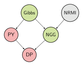
	$\begin{array}[]{c}\xrightarrow{\text{``Multinomialization''}}\\ \\ \xleftarrow{\text{Weak limit as }K\to\infty}\end{array}$
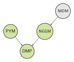
(a) BNP processes		(b) Multinomial processes

Figure 1: Graphical representation of the relationships between the discrete mixing measures considered in this article. An arrow indicates that the target is a special case of the origin. (a) BNP processes: Gibbs-type priors (Gibbs), normalized random measures with independent increments (NRMI), Pitman–Yor process (PY), normalized generalized gamma process (NGG), and Dirichlet process (DP). (b) Multinomial processes (finite-dimensional approximations of their respective BNP counterparts in the left panel): normalized infinitely divisible multinomial process (NIDM), Pitman–Yor multinomial process (PYM), normalized generalized gamma multinomial process (NGGM), and Dirichlet multinomial process (DMP). Going from left to right can be done according to a “multinomialization” of the BNP processes as described in Section 2.3, while the reverse direction is achieved by taking a weak limit as $K\to\infty$. Our contributions generalize results known for mixing measures in red to mixing measures in green. The case of mixing measures in gray remains an open problem.

2.4 Posterior consistency

Posterior consistency is an asymptotic property of the posterior. As in frequentist inference, we can consider that there exists a true value for the parameter of the distribution of the data. Then the posterior is said to be consistent if it converges to the true parameter as the sample size increases to infinity.

More formally, given a prior distribution $\pi$ on the parameter space $\Theta$, we denote by $\Pi(\cdot\mid X_{1:n})$ the posterior distribution with $X_{1:n}$ a given sample of the data. The posterior distribution is said to be consistent at $\theta_{0}\in\Theta$ if $\Pi(U^{c}\mid X_{1:n})\underset{n\to\infty}{\longrightarrow}0$ in $P_{\theta_{0}}$-probability for all neighborhoods $U$ of $\theta_{0}$. For instance, in our case, we consider mixture models for densities. In this type of model, the posterior density is said to be consistent at $f_{0}^{X}$ if, for a distance $d$ on the parameter space, $\Pi(d(f,f_{0}^{X})\geq\varepsilon\mid X_{1:n})\underset{n\to\infty}{\longrightarrow}0$ in $P_{f_{0}^{X}}$-probability for all $\varepsilon>0$. It is also possible to define posterior consistency for quantities of interest such as the number of clusters. The posterior number of clusters $K_{n}$ is said to be consistent at $K_{0}$ if $\Pi(K_{n}=K_{0}\mid X_{1:n})\underset{n\to\infty}{\longrightarrow}1$ in $P_{f_{0}^{X}}$-probability.

A refinement in the study of posterior consistency is to evaluate the speed at which a posterior distribution concentrates around the true parameter. The quantity which evaluates this speed is named a posterior contraction rate. More formally, the parameter space $\Theta$ is supposed to be a metric space with a metric $d$. A sequence $\varepsilon_{n}$ is a posterior contraction rate at the parameter $\theta_{0}$ with respect to the metric $d$ if for every $M_{n}\to\infty$, $\Pi(d(\theta,\theta_{0})\geq M_{n}\varepsilon_{n}\mid X_{1:n})\underset{n\to\infty}{\longrightarrow}0$ in $P_{\theta_{0}}$-probability.

For more details on posterior consistency or contraction rates, the reader could refer to Ghosal and Van der Vaart (2017, Chapters 6 to 9).

3 Inconsistency results

In this section, we generalize the inconsistency results by Miller and Harrison (2014). Under the context defined previously, Miller and Harrison (2014) states sufficient conditions that imply posterior inconsistency of the number of clusters and also proves that these conditions are satisfied for the Dirichlet process and Pitman–Yor process mixture models. For completeness, we first recall here this inconsistency result and then prove that it also applies to the different models introduced in Section 2.

3.1 Inconsistency theorem of Miller and Harrison (2014)

The central result of Miller and Harrison (2014, Theorem 6) is reproduced below as Theorem 1. This result depends on two conditions which are discussed thereafter.

We start with some notations. For $A\in\mathcal{A}_{k}(n)$, we define $R_{A}=\bigcup_{i:|A_{i}|\geq 2}A_{i}$, the union of all clusters except singletons. For index $j\in R_{A}$, we define $B(A,j)$ as the ordered partition $B\in\mathcal{A}_{k+1}(n)$ obtained by removing $j$ from its cluster $A_{\ell}$ and creating a new singleton for it. Then $B_{\ell}=A_{\ell}\setminus\{j\}$, and $B_{k+1}=\{j\}$. Let $\mathcal{Z}_{A}:=\{B(A,j):j\in R_{A}\}$, for $n>k\geq 1$, we define

$$c_{n}(k):=\frac{1}{n}\max_{A\in\mathcal{A}_{k}(n)}\max_{B\in\mathcal{Z}_{A}}\frac{p(A)}{p(B)},$$

with the convention that $0/0=0$ and $y/0=\infty$ for $y>0$.

Condition 1.

Assume $\limsup_{n\to\infty}c_{n}(k)<\infty$, given some particular $k\in\{1,2,\ldots\}$.

Miller and Harrison (2014) show that this condition holds for any $k\in\{1,2,\ldots\}$ for the Pitman–Yor process, and thus for the Dirichlet process.

The second condition, named Condition 4 in Miller and Harrison (2014), controls the likelihood through the control of single-cluster marginals. The single-cluster marginal for cluster $i$ is $m(X_{A_{i}})=\int_{\Theta}\left(\prod_{j\in A_{i}}f(X_{j}\mid\theta)\right)\pi(\theta)\mathrm{d}\theta$. This condition induces, for example, that as $n\to\infty$, there is always a non-vanishing proportion of the observations for which creating a singleton cluster increases its cluster marginal. This condition only involves the data distribution and is shown to hold for several discrete and continuous distributions, such as the exponential family (see Theorem 7 in Miller and Harrison, 2014). In the following, we assume that this condition is satisfied and mainly focus on Condition 1.

Theorem 1 (Miller and Harrison, 2014).

Let $X_{1},X_{2},\ldots\in\mathcal{X}$ be a sequence of random variables, and consider a partition-based model. Then, if Condition 4 from Miller and Harrison (2014) holds, and Condition 1 above holds for any $k\geq 1$, we have for any $k\geq 1$

$$\limsup_{n\to\infty}\Pi(K_{n}=k\mid X_{1:n})<1\;\text{ with probability }1.$$

As said previously, Condition 1 is only related to partition distribution, while Condition 4 from Miller and Harrison (2014) only involves the data distribution and single-cluster marginals. Hence, to generalize this inconsistency result to other processes, it is enough to show that Condition 1 also holds for these different processes. This is the focus of the next section, for Gibbs-type processes and for finite-dimensional discrete priors.

3.2 Inconsistency of Gibbs-type and multinomial processes

We extend the inconsistency result for all the processes introduced in Section 2 by proving that Condition 1 holds.

Proposition 1 (Gibbs-type processes).

Consider a Gibbs-type process with $0\leq\sigma<1$, then Condition 1 holds for any $k\in\{1,2,\ldots\}$, and so does the inconsistency of Theorem 1.

Proposition 2 (Multinomial processes).

Consider any of the following priors: Dirichlet multinomial process, Pitman–Yor multinomial process and normalized generalized gamma multinomial process, with $K$ components. Then Condition 1 holds for any $k<\min(n,K)$, and so does the inconsistency of Theorem 1.

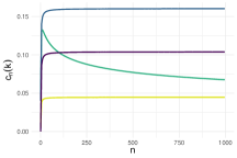
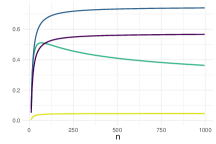
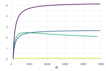
(a) $k=1$	(b) $k=10$	(c) $k=100$
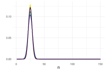
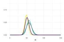
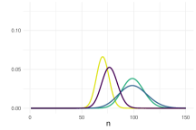
(d) $n=50$	(e) $n=250$	(f) $n=1000$

Figure 2: (Top row) Illustrations of Condition 1, for $k\in\{1,10,100\}$: the function $n\mapsto c_{n}(k)$ reaches a plateau for large values of $n$ for a range of priors (see infra).
(Bottom row) Prior probability on the number of clusters for different processes and different values of $n$. In both rows, parameters are fixed such that $\mathbb{E}[K_{50}]=25$: for Dirichlet process DP$(\alpha=19.2)$, for Pitman–Yor process py$(\sigma=0.25,\alpha=12.2)$, for NGG process NGG$(\sigma=0.25,\beta=48.4)$ and for Dirichlet multinomial process DMP$(\alpha=22.5,K=200)$. Illustrations are made using the package GibbsTypePriors (github.com/konkam/GibbsTypePriors).

The proofs of Propositions 1 and 2 are provided in Appendix A. Note that although the Dirichlet multinomial process is a particular case of the Pitman–Yor multinomial process and the normalized generalized gamma multinomial process, we include it as a separate case in the statement as the proof for this case differs from the proofs for its generalizations.

The top row of Figure 2 illustrates Condition 1 for different partition distributions, such as the Dirichlet multinomial process (DMP), the Dirichlet process (DP), the Gibbs-type process for the normalized generalized gamma process (NGG) special case and the Pitman–Yor process (PY). In all these cases, we represent the function $c_{n}(k)$ defined in Section 3 for different values of $k$, $k\in\{1,10,100\}$, with $n\in\{1,\ldots,5000\}$ and for some fixed parameters chosen such that $\mathbb{E}[K_{50}]=25$. We draw all the priors we considered for this choice of the parameters in Figure 2 bottom row. We also illustrate how the priors vary depending on $n$, fixing the priors parameters such that $\mathbb{E}[K_{50}]=25$ then we made $n$ varying, $n\in\{50,250,1000\}$. In Figure 2 top row, we can see $n\mapsto c_{n}(k)$ function reaches a plateau, thus indicating its boundedness for every process and values of $k$.

More precisely, the proof (as in Miller and Harrison, 2014, Proposition 5) consists in controlling the ratio of probability $\frac{1}{n}~{}p(A)/p(B)$, where $B=B(A,j)$ is defined in Section 3.1. For the Gibbs-type process, as the ratio of probability is raised by $(V_{n,k}/V_{n,k+1})$, it is enough to show that the sequence $(V_{n,k}/V_{n,k+1})_{n\geq 1}$ is bounded. Since there is no simple formula for $V_{n,k}$ in the general case of the Gibbs-type process, we prove this by using a Laplace approximation. The idea of the original proof of Miller and Harrison (2014) is the same but this ratio simplifies as they consider Pitman–Yor process.

For the Pitman–Yor multinomial process and the NGG multinomial process, the partition distribution depends on a sum over the vectors $\ell^{(k)}=(\ell_{1},\ldots,\ell_{k})$ such that $\ell_{i}\in\{1,\ldots,n_{i}\}$ and $|\ell^{(k)}|=\ell_{1}+\cdots+\ell_{k}$. We write this sum as $k$ different sums over each $\ell_{i}$. As in the nonparametric case, we consider the ratio of probability $\frac{1}{n}~{}p(A)/p(B)$. By definition of partition $B$, if $j\in A_{k}$ then the sum over $\ell_{k}$ is different for $p(A)$ and $p(B)$, one is of $n_{k}$ elements and the other of $n_{k}-1$ elements. We separate the sum of $n_{k}$ elements into two sums, the first one of $n_{k}-1$ elements and the second one of one element. In this way, we can use some known properties of the generalized factorial coefficients and some specific properties of each process to conclude.

4 Consistency results

The inconsistency results of the previous section show that the posterior number of clusters is not necessarily the most relevant quantity to consider when the number of clusters is a quantity of interest. Instead, results by Rousseau and Mengersen (2011); Nguyen (2013); Scricciolo (2014) suggest that it might be better to focus on the mixing measure. In particular, recent works on consistency can be extended to the models we consider. In this part, we consider the framework of Rousseau and Mengersen (2011) and investigate to which extent it might apply to some models we have been considering, the Dirichlet multinomial process and Pitman–Yor multinomial process mixture models. Guha et al. (2021) introduced a post-processing procedure, the Merge-Truncate-Merge (MTM) algorithm, for which the output, the number of clusters, is consistent. Guha et al. (2021) proved that this algorithm can be applied to the Dirichlet process mixture model so that there is consistency for the number of clusters after applying this algorithm. We extend this result and prove that we can apply the algorithm to overfitted mixture models and to the Pitman–Yor process mixture model.

4.1 Emptying extra clusters

Overfitted mixtures can be constructed based on the Dirichlet multinomial process or the Pitman–Yor multinomial process. Rousseau and Mengersen (2011) show in their Theorem 1 that overfitted mixtures, under some conditions on the kernel and the mixture model, have the desirable property that in the mixing measure the weights of extra components tend to zero as the sample size grows. This result only concerns the weights and not the number of clusters, but a near-optimal posterior contraction rate for the mixing measure can be deduced from it (see section 3.1 in Guha et al., 2021). To be more precise, Rousseau and Mengersen (2011) consider a prior $\pi$ on the mixture weights $w$ written as follows

$$\pi(w)=C(w)w_{1}^{\alpha_{1}-1}\cdots w_{k}^{\alpha_{k}-1},$$

with specific properties for the function $C(w)$ recalled in Condition 3. Two types of prior hyper-parameter configurations are studied, which lead to opposite conclusions: merging or emptying of extra components. Let $d$ be the dimension of the component-specific parameter $\theta$. If $\bar{\alpha}=\min_{j}(\alpha_{j})$ is such that $\bar{\alpha}<d/2$, then the posterior expectation for the weights of the extra components tends to zero. This is the case where extra components are emptied. The other case corresponds to $\bar{\alpha}>d/2$. In this case, the extra components are merged with non-negligible weight, which means that they become identical to an existing component and inadvertently borrow some of its weight. This case is less stable as there are different merging possibilities. It is therefore preferable to choose parameters of the prior that belong to the first case. The result stated in Theorem 1 in Rousseau and Mengersen (2011), depends on five conditions. The first one is a posterior contraction condition on the mixture density. Conditions 2, 3, and 4 are some standard conditions on the kernel density, respectively on regularity, integrability, and strong identifiability. The last condition concerns the prior which needs to have some classic properties.

To apply Theorem 1 in Rousseau and Mengersen (2011) to our case, as the kernel is not the focus of this article, the only conditions we need to check are the conditions on the mixture model. We recall here these two conditions, which correspond to the condition on the posterior contraction of the mixing measure and the one on the prior.

Condition 2 (Rousseau and Mengersen, 2011, Condition 1).

There exists $\varepsilon_{n}\leq\log(n)^{q}/\sqrt{n}$, for some $q\geq 0$, such that

$$\lim_{M\to\infty}\limsup_{n}\left\{\mathbb{E}^{n}_{0}\left[\Pi(\|f^{X}-f_{0}^{X}\|_{1}\geq M\varepsilon_{n}\mid X_{1:n})\right]\right\}=0,$$

where $f_{0}^{X}$ is the true mixture density.

Condition 3 (Rousseau and Mengersen, 2011, Condition 5).

The prior density with respect to Lebesgue measure on the cluster-specific parameter $\theta$ is continuous and positive on $\Theta$, and the prior $\pi(w)$ on $w=(w_{1},\ldots,w_{K})$ satisfies

$$\pi(w)=C(w)w_{1}^{\alpha_{1}-1}\cdots w_{K}^{\alpha_{K}-1},$$

where $C(w)$ is a continuous function on the simplex bounded from above and from below by positive constants.

Proposition 3.

Assume that the kernel considered satisfies Conditions 2, 3, and 4 of Theorem 1 in Rousseau and Mengersen (2011). Let $G$ be a Dirichlet multinomial process or a Pitman–Yor multinomial process with parameter $\sigma=1/2$. Then, Conditions 2 and 3 are satisfied, and Theorem 1 of Rousseau and Mengersen (2011) holds.

The proof of this proposition can be found in Appendix B. It relies on Theorem 4.1 from Rousseau et al. (2019) through which Condition 2 holds for mixture models based on the Dirichlet multinomial process or the Pitman–Yor multinomial process. This theorem gives a result on density consistency for finite mixture models in the exact setting, which remains true in the overfitted mixture case.

The proof in Appendix B consists mainly in proving that Condition 3 holds true for the different priors we consider. In the Pitman–Yor multinomial case, we are able to prove that Condition 3 holds only for $\sigma=1/2$. Indeed, $\sigma=1/2$ is the only value for which the prior on the weights, a ratio-stable distribution, has a closed-form density. Therefore, it is interesting to choose $\sigma=1/2$ when using the Pitman–Yor multinomial process, as we want at least to be in the case where Proposition 3 applies. In this case, Theorem 1 from Rousseau and Mengersen (2011) applies which ensures that the weights of extra components tend to zero when $\bar{\alpha}<d/2$.

However, note that the condition $\bar{\alpha}<d/2$ is more restrictive for the Pitman–Yor multinomial process with parameters $\bar{\alpha}$ and $\sigma=1/2$, than for Dirichlet multinomial process with parameter $\alpha$. Indeed, in the former case $\bar{\alpha}=\tilde{\alpha}+\frac{K-1}{2}$ (see proof in Section B), so condition $\tilde{\alpha}+\frac{K-1}{2}<d/2$ imposes a restriction on the choice of $K$ in addition to that on $\bar{\alpha}$. For example, if $d=2$ (e.g. 1D location-scale mixtures) then $K\leq 2$. This means that a Pitman–Yor multinomial model is likely to be in the merging regime, $\bar{\alpha}>d/2$. Conversely, in the case of the Dirichlet multinomial process, there is no restriction on $K$. Thus, it is always possible to be in the first regime where $\bar{\alpha}<d/2$ and extra components are emptied.

4.2 Merge-Truncate-Merge

We assume throughout this section as in Guha et al. (2021) that the parameter space $\Theta$ is compact. We denote by $W_{r}(\cdot,\cdot)$ the Wasserstein distance of order $r$, $r\geq 1$. We recall in Theorem 2 the following result by Guha et al. (2021).

Theorem 2 (Guha et al., 2021, Theorem 3.2.).

Let $G$ be a posterior sample from the posterior distribution of any Bayesian procedure, namely $\Pi(\cdot\mid X_{1:n})$ such that for all $\delta>0$

$$\Pi\left(G\,:\,W_{r}(G,G_{0})\leq\delta\omega_{n}\mid X_{1:n}\right)\overset{p_{G_{0}}}{\longrightarrow}1,$$

with $\omega_{n}=o(1)$ a vanishing rate, $r\geq 1$. Let $\tilde{G}$ and $\tilde{K}$ be the outcome of the Merge-Truncate-Merge algorithm (Guha et al., 2021) applied to $G$. Then the following hold as $n\to\infty$.

1. $\Pi(\tilde{K}=K_{0}\mid X_{1:n})\longrightarrow 1$ in $P_{G_{0}}$-probability.

2. For all $\delta>0$, $\Pi(G\,:\,W_{r}(\tilde{G},G_{0})\leq\delta\omega_{n}\mid X_{1:n})\longrightarrow 1$ in $P_{G_{0}}$-probability.

Proposition 4 (Pitman–Yor process).

Let $G$ be a posterior sample from the posterior distribution of a Pitman–Yor process mixture. Under conditions of Lemma 1, Theorem 2 applies to $G$.

Proposition 5 (Overfitted mixtures).

Let $G$ be a posterior sample from the posterior distribution of an overfitted mixture. Under conditions of second-order identifiability and uniform Lipschitz continuity of the kernel (Nguyen, 2013; Ho and Nguyen, 2016), Theorem 2 applies to $G$ with $r\leq 2$.

To prove Proposition 4, we introduce a lemma which derives from Theorem 1 in Scricciolo (2014). The conditions of this theorem are three standard conditions (A1)-(A3). (A1) is a condition on the kernel density, (A2) is a tail condition on the true mixing distribution, and (A3) is a condition on the base measure. To state this lemma, we also need another condition on the kernel $f(\cdot\mid\theta)$. We suppose that for some constants $0<\rho<\infty$ and $0<\eta\leq 2$, the Fourier transform $\hat{f}$ of $f(\cdot\mid\theta)$ satisfies $|\hat{f}(t)|\sim e^{-\left(\rho|t|\right)^{\eta}}$

Lemma 1.

Under the conditions above and by assuming $\Theta$ bounded, with $G$ the posterior mixing measure of a Pitman–Yor process mixture model, with $\sigma\in[0,1)$, then for every $1\leq r<\infty$, there exists a sufficiently large constant $M$ and some $0<\eta\leq 2$ such that

$$\Pi(G:W_{r}(G,G_{0})\geq M(\log n)^{-1/\eta}\mid X^{(n)})\to 0\text{ in }P_{G_{0}}\text{-probability.}$$

The proof of this lemma can be found in Appendix B. This lemma is similar to Corollary 2 from Scricciolo (2014) which applies to the special case of the Dirichlet process. With this lemma, we can now prove Proposition 4.

Proof of Proposition 4.

Theorem 2 holds when the posterior $G$ is such that for all $\delta>0$, there exists a vanishing rate $\omega_{n}$ such that

$$\Pi\left(G\,:\,W_{r}(G,G_{0})\geq\delta\omega_{n}\mid X_{1:n}\right)\longrightarrow 0\text{ in }P_{G_{0}}\text{-probability}.$$

Under the conditions of Lemma 1, we have

$$\Pi(G:W_{r}(G,G_{0})\geq M(\log n)^{-1/\eta}\mid X_{1:n})\to 0\text{ in }P_{G_{0}}\text{-probability,}$$

so that $\delta\omega_{n}=M(\log n)^{-1/\eta}$.

Hence, the consistency results of Theorem 2 hold for a Pitman–Yor process mixture model satisfying the conditions of Lemma 1. ∎

In the case of Proposition 5, we also need a contraction rate for the mixing measure of overfitted mixture models. Let $G$ be the mixing measure of any overfitted mixture model. It is known that under some conditions on the kernel there exists a rate of contraction for $G$ (see Equation (5) Guha et al., 2021),

$$\Pi\left(G\,:\,W_{2}(G,G_{0})\gtrsim(\log n/n)^{1/4}\mid X_{1:n}\right)\longrightarrow 0\text{ in }P_{G_{0}}\text{-probability}.$$ (10)

This rate can be suboptimal for some overfitted mixture models but is sufficient to prove Proposition 5.

Proof of Proposition 5.

The proof of Theorem 2 is the same in the case of overfitted mixtures as in the Bayesian nonparametric case. This theorem holds when the posterior $G$ is such that for all $\delta>0$, there exists a vanishing rate $\omega_{n}$ such that

$$\Pi\left(G\,:\,W_{r}(G,G_{0})\geq\delta\omega_{n}\mid X_{1:n}\right)\longrightarrow 0\text{ in }P_{G_{0}}\text{-probability}.$$

We use Equation (10) to conclude with $\delta\omega_{n}\leq(\log n/n)^{1/4}$ and $r=2$.

Hence, the consistency results of Theorem 2 hold for a Pitman–Yor process mixture model satisfying the conditions of Lemma 1. ∎

The work of Guha et al. (2021) can be applied to different Bayesian procedures. The only condition is to have a contraction rate for the mixing measure under the Wasserstein distance. However, this condition is not easy to prove, here we prove it for the Pitman–Yor process but there is no direct generalization for Gibbs-type processes. In the overfitted mixtures case, there is a general contraction rate for the mixing measure under the Wasserstein distance (see Nguyen, 2013; Ho and Nguyen, 2016). This rate could be suboptimal for some procedures as it is an upper bound but it guarantees the consistency of the Merge-Truncate-Merge algorithm.

5 Simulation study

We consider a simulation study to illustrate the three parts of our theoretical results pertaining to (i) inconsistency of the posterior distribution of $\tilde{K}_{n}$ (Section 3.2), (ii) emptying of extra clusters (Section 4.1), and (iii) the Merge-Truncate-Merge algorithm (Section 4.2). We study the familiar case of a Dirichlet multinomial mixture of multivariate normals. The simulated data was generated using a Gaussian location mixture, with a parameter setting similar to the one of Guha et al. (2021) for the Dirichlet Process. More precisely, we have $K_{0}=3$ clusters and Gaussian kernels such that:

$$f(x)=\sum_{i=1}^{3}w_{i}\mathcal{N}(x\mid\mu_{i},\Sigma),$$

where $w=(w_{1},w_{2},w_{3})$ are the weights, which we fix as $w=(0.5,0.3,0.2)$, and $N(x\mid\mu_{i},\Sigma)$ is a multivariate Gaussian distribution with mean $\mu_{i}$ and covariance matrix $\Sigma$. We considered the following parameters for the mean and the covariance matrix:

$$\mu_{1}=(0.8,0.8),\mu_{2}=(0.8,-0.8),\mu_{3}=(-0.8,0.8)\text{ and }\Sigma=0.05I_{2}.$$

Here, the dimension of the kernel parameter $\theta=(\mu,\Sigma)$ is $d=5$ (2 for $\mu$ and 3 for $\Sigma$). In this setting, we generated a sequence of datasets with $n=\{20,200,2000,20000\}$, such that the smaller datasets are subsets of the larger ones. The number of components of the Dirichlet multinomial process is set to $K=10$, thus satisfying the overfitted condition $K\geq K_{0}$. We chose the maximum parameter of the Dirichlet distribution, $\bar{\alpha}=\alpha/K$, according to the intuition of Rousseau and Mengersen (2011) results. To obtain vanishing weights for extra components, the parameter $\bar{\alpha}$ should be less than $d/2=2.5$. We consider the following values: $\bar{\alpha}\in\{0.01,1,2.5,3\}$. We used the Markov chain Monte Carlo (MCMC) sampler proposed by Malsiner-Walli et al. (2016). Although the proposed algorithm allows using a hyperprior on the parameter $\alpha$ and shrinkage priors on the component means, we have used the basic version with standard priors on parameters (see details in Appendix C). Also in Appendix C, we further the investigation and consider cases where parameter $\bar{\alpha}$ is not fixed. Two situations are considered. In the first case, the prior expected number of clusters is fixed, which leads to decreasing parameter $\alpha$ at a rate asymptotically equivalent to $\log(n)^{-1}$. In the second case, we introduce a prior distribution on $\bar{\alpha}$.

Posterior inconsistency on $\tilde{K}_{n}$

In Figure 3, we present the posterior distribution of the number of clusters for different values of parameter $\bar{\alpha}$ and different sizes of the dataset $n$. In addition, we present the prior distribution on the number of clusters for the corresponding $\bar{\alpha}$ and $n$. Table 2 summarizes the values of the parameters $\bar{\alpha}$ and sample sizes $n$ used in the simulation study and displays the associated prior and posterior expected number of clusters $K_{n}$. As proved in Proposition 2, the posterior distribution diverges with $n$. This divergence is visible for the all considered values $\bar{\alpha}\in\{0.01,1,2.5,3\}$ in our experiments. However, for $\bar{\alpha}=0.01$, the posterior distribution stays concentrated around the true value $K_{0}=3$ for the range of sample sizes $n$, except $n=20000$. Interestingly, Figure 3 makes it clear that the prior with fixed $\bar{\alpha}$ puts increasing mass towards $K_{n}=10$ as the sample size grows, which is probably one of the root causes for posterior inconsistency. Allowing $\bar{\alpha}$ to vary, as investigated on Figure 7 in Appendix C, induces a much less informative prior on the number of clusters and the posterior deterioration as the sample size grows appears much less striking.

Emptying of extra clusters

We are also interested to see how the posterior distribution of the component weights behaves in our simulation setting. Figure 4 illustrates the posterior distribution of the weights of the components for different specifications of the parameter $\bar{\alpha}$ and $n$, and is similar to Figure 1 and Figure 2 in Rousseau and Mengersen (2011). In our case, we sort the weights in decreasing order to alleviate the label-switching problem. For the very small values of $\bar{\alpha}=0.01$, we can see that the posterior weights with growing $n$ are concentrated at the true values of mixture weights, except the largest $n$. When $\bar{\alpha}=1$, we can observe the concentration trend, but convergence is slower than in the first case. For $\bar{\alpha}=2.5$ there is no clear dynamics. And for $\bar{\alpha}=3$ we can see that the weights become more uniformly distributed, which can be related to the merging weights regime. Specification of our simulation study does not allow to apply the Rousseau and Mengersen (2011) theory directly, as in our case the support of $\theta$ is not bounded. However, we can see that the simulation results are still consistent with the theory, suggesting wider applicability.

Merge-Truncate-Merge.

We applied the Merge-Truncate-Merge algorithm proposed by Guha et al. (2021) to the posterior distribution of the mixing measure in our simulation setting and illustrate the posterior distribution of the number of clusters $\tilde{K}$ on Figure 5. To use the Merge-Truncate-Merge algorithm, we need to know the Wasserstein convergence rates of the corresponding mixing measure. We use the convergence rate for overfitted mixtures $\omega_{n}=(\log(n)/n)^{1/4}$ (Guha et al., 2021). Note that for this convergence rate the prior on the kernel parameters should be bounded, which is not the case in our simulation (see details in Appendix C), so as in the previous section, we apply Merge-Truncate-Merge out of its theoretically proven domain. The Merge-Truncate-Merge algorithm depends on the specification of a positive scalar $c$. As there is no explicit guideline for computing $c$, we tested a range of values $c\in\{0.1,0.5,1,2\}$, see Figure 5. We can note that for each value of $n$, there exists some value of $c$ such that the posterior distribution of the number of clusters remains concentrated around the true number of components $K_{0}=3$. At the same time, some values of $c$ are too restrictive or do not eliminate extra clusters. For example, $c=0.01$ for $\bar{\alpha}=1$ does not allow the number of components to be correctly estimated. Conversely, too large value of $c$ makes the Merge-Truncate-Merge algorithm also fail in the sense that it outputs zero values for $\tilde{K}$. This is due to the fact that the truncate step truncates all clusters at once. This suggests interpreting $c$ as a regularization parameter, with the estimated number of clusters decreasing with increasing $c$. Following this intuition, we can draw (Figure 6) so-called “regularization paths” plots for $c$. More specifically, they represent the posterior mean and maximum a posteriori (MAP) for the posterior distribution of $\tilde{K}$ for a range $c\in[0.01,2]$. We can see that for all specifications of parameter $\bar{\alpha}$ for large $n\geq 2000$, there always exists a region where the posterior mean and the MAP remain approximately constant (exactly constant for the MAP). This suggests a heuristic to use the Merge-Truncate-Merge algorithm: calibrate a grid of $c$ values such that for $c_{\min}$ the estimated number of clusters is close to $K$, for $c_{\max}$ the estimated number of clusters is 0, then explore regularly spaced values in $[c_{\min},c_{\max}]$ and look for a plateau. In the absence of a plateau the sample size should be increased.

$n$	Prior $\mathbb{E}[K_{n}]$				Posterior $\mathbb{E}[K_{n}|X_{1:n}]$
	$\bar{\alpha}=0.01$	$\bar{\alpha}=1$	$\bar{\alpha}=2.5$	$\bar{\alpha}=3$	$\bar{\alpha}=0.01$	$\bar{\alpha}=1$	$\bar{\alpha}=2.5$	$\bar{\alpha}=3$
20	1.3	6.9	7.9	8	2.7	4.9	5.8	6.0
200	1.5	9.6	9.9	9.98	3.03	6.8	9.4	9.7
2000	1.7	9.9	$\approx$ 10	$\approx$ 10	3.02	8.0	9.98	9.99
20000	1.9	9.99	$\approx$ 10	$\approx$ 10	3.05	8.8	$\approx$ 10	$\approx$ 10

Table 2: Prior and posterior expected number of clusters $K_{n}$ for the various values of $\bar{\alpha}$ considered in our experiments.

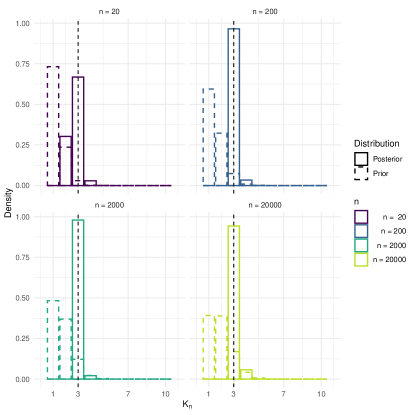
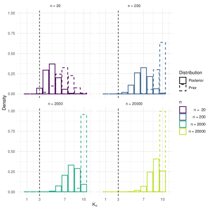
(a) Fixed $\bar{\alpha}=0.01$	(b) Fixed $\bar{\alpha}=1$
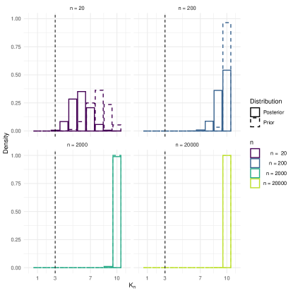
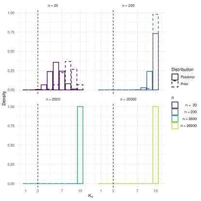
(c) Fixed $\bar{\alpha}=2.5$	(d) Fixed $\bar{\alpha}=3$

Figure 3: Prior and posterior distributions of the number of clusters $K_{n}$ under a Dirichlet multinomial process mixture with fixed parameter $K=10$, and various choices of $\bar{\alpha}=\alpha/K$ and $n$. The value $\bar{\alpha}=2.5$ corresponds to Rousseau and Mengersen (2011)’s threshold.

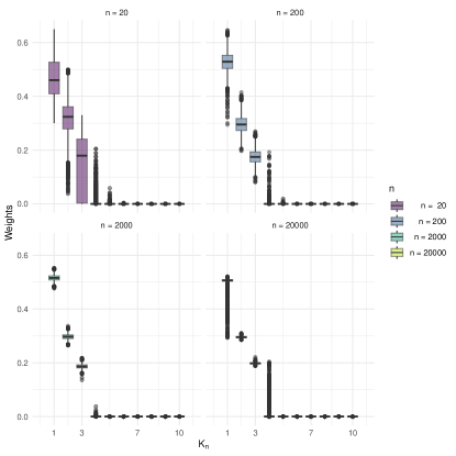
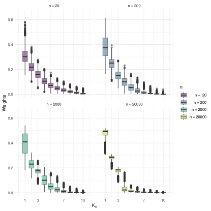
(a) Fixed $\bar{\alpha}=0.01$	(b) Fixed $\bar{\alpha}=1$
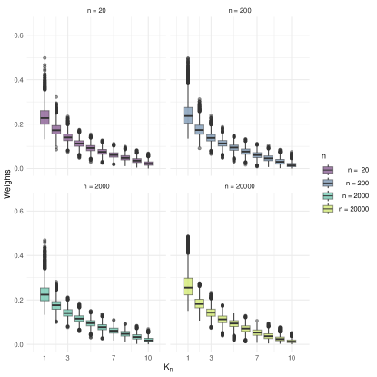
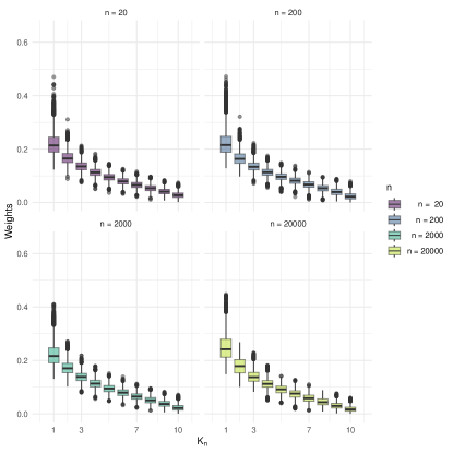
(c) Fixed $\bar{\alpha}=2.5$	(d) Fixed $\bar{\alpha}=3$

Figure 4: Mixture weights under a Dirichlet multinomial process mixture with fixed parameter $K=10$, and various choices of $\bar{\alpha}=\alpha/K$ and $n$.

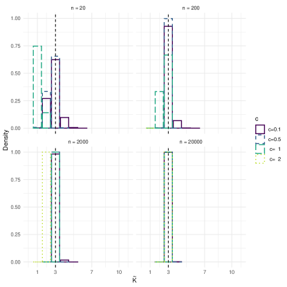
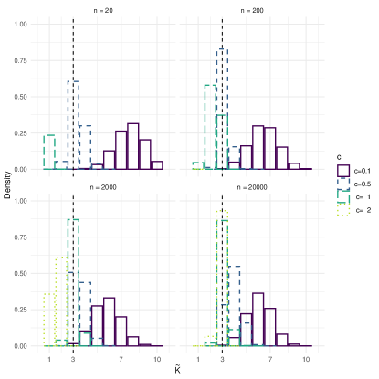
(a) Fixed $\bar{\alpha}=0.01$	(b) Fixed $\bar{\alpha}=1$
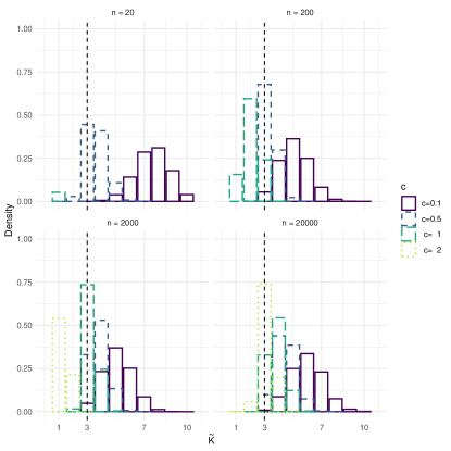
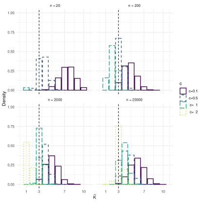
(c) Fixed $\bar{\alpha}=2.5$	(d) Fixed $\bar{\alpha}=3$

Figure 5: Distribution of $\tilde{K}$, that is the posterior number of clusters after applying the Merge-Truncate-Merge algorithm of Guha et al. (2021), with $c$ parameter in $\{0.1,0.5,1,2\}$, under a Dirichlet multinomial process mixture with fixed parameter $K=10$, and various choices of $\bar{\alpha}=\alpha/K$ and $n$.

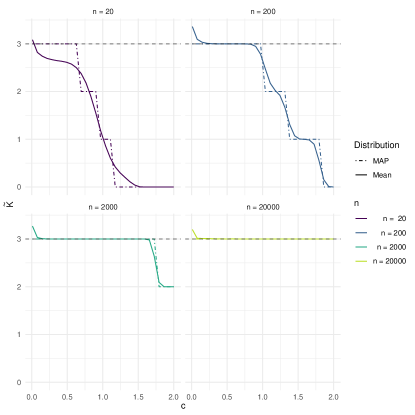
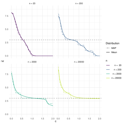
(a) Fixed $\bar{\alpha}=0.01$	(b) Fixed $\bar{\alpha}=1$
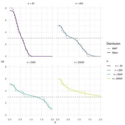
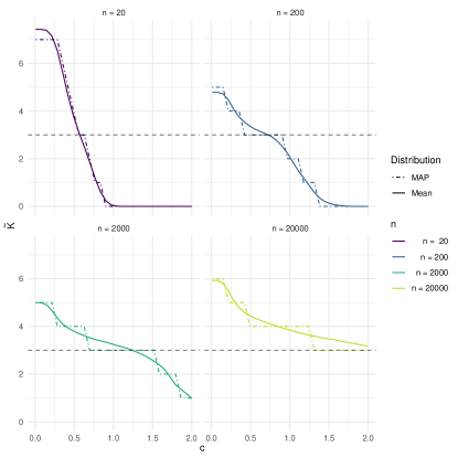
(c) Fixed $\bar{\alpha}=2.5$	(d) Fixed $\bar{\alpha}=3$

Figure 6: “Regularization path” for $\tilde{K}$, that is the posterior number of clusters after applying the Merge-Truncate-Merge algorithm of Guha et al. (2021), with $c$ parameter in $[0,2]$, under a Dirichlet multinomial process mixture with fixed parameter $K=10$, and various choices of $\bar{\alpha}=\alpha/K$ and $n$. The solid curves represent the posterior mean while the dotted dashed curves represent the maximum a posteriori (MAP) and the dotted horizontal line represents $K_{0}=3$.

6 Discussion

We studied the finite and infinite mixture models with well-specified kernels applied to data generated from a mixture with a finite number of components. In this setting, we have proved that Gibbs-type process mixtures are inconsistent a posteriori for the number of clusters. It is also the case for some finite-dimensional representations of Gibbs-type priors as the Dirichlet multinomial, Pitman–Yor multinomial and normalized generalized gamma multinomial processes. However, we did not prove inconsistency in general for NIDM (Lijoi et al., 2020a). Further, we discussed the different approaches to solving inconsistency problems for both finite and infinite mixtures.

For overfitted mixtures, Rousseau and Mengersen (2011) prove that for some parameter specifications the weights for extra components vanish, but it does not guarantee the posterior consistency of the number of clusters. We show that this guides prior specification for some of the models which are inconsistent a posteriori, such as overfitted mixtures based on the Dirichlet multinomial and Pitman–Yor multinomial processes. In the case of Pitman–Yor multinomial process mixtures this requires a parameter specification that can be restrictive. When the Wasserstein convergence rate of the mixing measure is known, the Merge-Truncate-Merge (MTM) algorithm proposed by Guha et al. (2021) allows obtaining a consistent estimate of the number of components in Bayesian nonparametric and overfitted mixtures. In particular, we showed that in contrast to the results of Rousseau and Mengersen (2011), the Merge-Truncate-Merge algorithm can be applied to the Dirichlet multinomial and Pitman–Yor multinomial processes without parameters constraints. Moreover, we also proved that Merge-Truncate-Merge can be applied to Pitman–Yor process.

Even if it seems possible to recover some consistency with for example the Merge-Truncate-Merge procedure, the inconsistency results suggest that Gibbs-type process mixture models face challenges when employed to estimate a finite number of components. This can be related to the fact that this usage corresponds to model misspecification, as these models assume an infinite number of components or a number of clusters growing with the sample size. When it is known that the number of components is finite, we can also use a Mixture of Finite Mixtures which is better specified for this case. With MFM, there is consistency for the number of components as proved in Guha et al. (2021). However, MFM have a reputation for being more computationally challenging than the Dirichlet process mixture, for instance, when the number of components is large (see remark in Section 3.2 Guha et al., 2021). This might be a motivation to favor using misspecified Gibbs-type process mixture models in conjunction with the Merge-Truncate-Merge algorithm for instance in place of MFM. However, recent works introduced new samplers for MFM which appear more computationally efficient than the usual ones (Miller and Harrison, 2018; Frühwirth-Schnatter et al., 2021).

It is known that the Dirichlet process mixture model tends to create some extra little clusters which are linked to the inconsistency result (see eg Miller and Harrison, 2014, and references therein). To avoid these clusters, some authors propose to use repulsive mixture models (see eg Petralia et al., 2012). Such models introduce a dependence on the components to better spread them out in the parameter space. Xie and Xu (2020) prove consistency for the density and the mixing measure for repulsive mixture models with Gaussian kernel. As for the number of components, no consistency is proven, but it is shown that some shrinkage effect occurs.

Another way to solve the inconsistency problem of the posterior number of clusters in the Dirichlet process mixture is introduced by Ohn and Lin (2022). Their solution is to make the concentration parameter $\alpha$ decrease when the sample size increases. With this assumption, they obtain a nearly tight upper bound on the true number of clusters through the posterior number of clusters. They also present a simulation study showing posterior consistency for the number of components. We can wonder if control over the concentration parameter $\alpha$ when the sample size increases can allow posterior consistency for the number of components. Indeed, Ascolani et al. (2022) proposes a way to control this parameter through a prior which gives consistency for the number of components for a Dirichlet process mixture. We investigate empirically these two directions in Appendix C. This provides a simulation study for Dirichlet multinomial mixtures where (i) we fix the expected number of clusters a priori when the sample size increases, implying that $\alpha$ decreases (Figure 7 (a) and (b)) and (ii) we use a Gamma prior on the concentration parameter (Figure 7 (c) and (d)). As illustrated in Figure 7, the posterior number of clusters in both cases seems to estimate the true number of components well even for large sample sizes, and the posterior seems to be consistent. However, there are no theoretical guarantees for consistency or inconsistency as the results of respectively Ohn and Lin (2022) and Ascolani et al. (2022) do not apply in both cases.

Another way to estimate the number of components is to use the approach of Wade and Ghahramani (2018). This approach consists of a point estimation of the partition of the data and is commonly used in practice. As it is widely used in practice, it would be interesting to investigate the consistency in this case.

Supporting Information

Additional information for this article is available online, corresponding to the code used for the simulations and the figures.

Appendix A Proofs of the results of Section 3

Proof of Proposition 1.

For all $k\in\{1,2,\ldots\}$, we want to prove that

$$\limsup_{n\to\infty}c_{n}(k)=\limsup_{n\to\infty}\frac{1}{n}\max_{A\in\mathcal{A}_{k}(n)}\max_{B\in\mathcal{Z}_{A}}\frac{p(A)}{p(B)}<\infty,$$

where $\mathcal{Z}_{A}$ and $\mathcal{A}_{k}(n)$ are defined in Section 2.1.
So, it is sufficient to prove that for any fixed $k$, there exists a constant $C$ such that for any $n$, for all $A\in\mathcal{A}_{k}(n)$ and $B=B(A,j)$ with $j\in A_{\ell}$, $\frac{1}{n}\frac{p(A)}{p(B)}\leq C$.

We consider the Gibbs-type prior case with $\sigma>0$, as case, $\sigma=0$ is a Dirichlet process and is already proven in Miller and Harrison (2014). As we are in the Gibbs-type prior case, we have, for $A\in\mathcal{A}_{k}(n)$, $p(A)=\frac{V_{n,k}}{k!}\prod_{i=1}^{k}(1-\sigma)_{n_{i}-1}$, and so

$$\frac{1}{n}\frac{p(A)}{p(B)} =\frac{1}{n}\frac{V_{n,k}}{k!}\prod_{i=1}^{k}(1-\sigma)_{|A_{i}|-1}\frac{(k+1)!}{V_{n,k+1}}\left(\prod_{i=1}^{k+1}(1-\sigma)_{|B_{i}|-1}\right)^{-1}$$

$$=\frac{k+1}{n}\frac{V_{n,k}}{V_{n,k+1}}\underbrace{(1-\sigma+|A_{\ell}|-2)}_{\leq n}$$

$$\leq\frac{V_{n,k}}{V_{n,k+1}}(k+1).$$

Therefore, we just have to prove that the sequence $\left(\frac{V_{n,k}}{V_{n,k+1}}\right)_{n\geq 1}$ is bounded.

Using the recurrence relation (3), we have

$$V_{n,k}=V_{n+1,k+1}+(n-\sigma k)V_{n+1,k} \iff\frac{V_{n,k}}{V_{n+1,k+1}}=\frac{V_{n+1,k+1}}{V_{n+1,k+1}}+(n-\sigma k)\frac{V_{n+1,k}}{V_{n+1,k+1}}$$

$$\iff\frac{V_{n+1,k}}{V_{n+1,k+1}}=\left(\frac{V_{n,k}}{V_{n+1,k+1}}-1\right)\frac{1}{n-\sigma k}.$$ (11)

We denote by $f_{n}(p,t)=t^{-\sigma k}p^{n-1-k\sigma}h(t)f_{\sigma}(t(1-p))$ the integrand function of Equation (4). From the definition of the $V_{n,k}$ in (4), we can write

$$\frac{V_{n+1,k}}{V_{n,k}}=\frac{1}{n-\sigma k}\frac{\iint pf_{n}}{\iint f_{n}}.$$

Using again the recurrence relation (3), we have

$$\frac{V_{n+1,k+1}}{V_{n,k}}=1-(n-\sigma k)\frac{V_{n+1,k}}{V_{n,k}}.$$

Then, applying the Laplace approximation method twice and by setting $(t_{n},p_{n})$ the mode of $f_{n}$, we obtain as in Arbel and Favaro (2021)

$$\frac{V_{n+1,k+1}}{V_{n,k}}=g(t_{n},p_{n})+o\left(\frac{1}{n}\right),$$ (12)

with $g(t_{n},p_{n})=1-p_{n}$. Indeed, to use the Laplace approximation, we write the integrand as $f_{n}=e^{n\ell_{n}}$, then

$$\frac{V_{n+1,k+1}}{V_{n,k}}=\frac{\iint ge^{n\ell_{n}}}{\iint e^{n\ell_{n}}}.$$

As the exponential term is the same in both integrands of this ratio, by applying the Laplace approximation method to both integrals, we obtain

$$\frac{V_{n+1,k+1}}{V_{n,k}}=\frac{g(t_{n},p_{n})+a(t_{n},p_{n})/n+\mathcal{O}\left(\frac{1}{n^{2}}\right)}{1+\mathcal{O}\left(\frac{1}{n}\right)},$$

where $a(t_{n},p_{n})$ is a second order term such that $a(t_{n},p_{n})=o(1/n)$. Hence, the previous ratio finally simplifies to (12).

Let $\varphi_{h}(t)=-th^{\prime}(t)/h(t)$, we can finally write using the partial derivatives above

$$\frac{V_{n+1,k+1}}{V_{n,k}}=\frac{\sigma k+\varphi_{h}(t_{n})}{n+\varphi_{h}(t_{n})-1}+o\left(\frac{1}{n}\right).$$ (13)

Thus, if $\varphi_{h}(t_{n})$ converges as $n$ tends to infinity, we have that $\frac{V_{n+1,k+1}}{V_{n,k}}\times\frac{n}{\sigma k}\to 1$ as $n\to\infty$, so with the relation (11), $\frac{V_{n+1,k}}{V_{n+1,k+1}}\underset{n\to\infty}{\longrightarrow}\frac{1}{\sigma k}$. If $\varphi_{h}(t_{n})$ diverges as $n$ tends to infinity, we have that

$$\lim_{n\to\infty}\frac{V_{n+1,k+1}}{V_{n,k}}=\left\{\begin{array}[]{ll}\frac{1}{c+1}&\text{ if }\frac{n}{\varphi_{h}(t_{n})}\underset{n\to\infty}{\longrightarrow}c,\;c\in\mathbb{R},\\ 0&\text{ if }\frac{n}{\varphi_{h}(t_{n})}\underset{n\to\infty}{\longrightarrow}\pm\infty.\end{array}\right.$$

And then, using again (11), $\frac{V_{n+1,k}}{V_{n+1,k+1}}\underset{n\to\infty}{\longrightarrow}0$. Hence,

$$\lim_{n\to\infty}\frac{V_{n+1,k}}{V_{n+1,k+1}}=\left\{\begin{array}[]{ll}\frac{1}{\sigma k}&\text{ if }\varphi_{h}(t_{n})\text{ converges,}\\ 0&\text{ if }\varphi_{h}(t_{n})\text{ diverges.}\end{array}\right.$$

Thus, the sequence $\left(\frac{V_{n,k}}{V_{n,k+1}}\right)_{n\geq 1}$ is bounded and Condition 1 is satisfied.

∎

Proof of Proposition 2.

We consider $A\in\mathcal{A}_{k}(n)$ and $B=B(A,j)$, and we assume for simplicity, and without loss of generality, that the cluster in $A$ which contains the element $j$ is the $k$-th cluster $A_{k}$. As in the previous proof, we want to bound the ratio $\frac{p(A)}{p(B)}$ for the three different partition probabilities considered in the proposition.

First, we consider the Dirichlet multinomial process, which is a special case of the Pitman–Yor multinomial process and normalized generalized gamma when $\sigma=0$. Then we consider the Pitman–Yor multinomial process and the normalized generalized gamma process with $\sigma>0$.

(a) Dirichlet multinomial process: using (8), we have

$$\frac{1}{n}\frac{p(A)}{p(B)}=\frac{1}{n}\frac{p(n_{1},\ldots,n_{k})}{p(n_{1},\ldots,n_{k}-1,1)}.$$

So,

$$\frac{1}{n}\frac{p(A)}{p(B)} =\frac{1}{n}\frac{(k+1)!(K-k-1)!\prod_{j=1}^{k}(c/K)_{n_{j}}(c)_{n}}{k!(K-k)!\prod_{i=1}^{k+1}(c/K)_{n_{i}}(c)_{n}}$$

$$=\frac{(k+1)(c/K+n_{k}-1)}{n(K-k)c/K}\leq\frac{K(k+1)}{c(K-k)}.$$

Thus, Condition 1 is satisfied for the Dirichlet multinomial process.

(b) Pitman–Yor multinomial process with $\sigma>0$: we denote by $q_{\ell^{(k)}}=\prod_{i=1}^{k}C(n_{i},\ell_{i};\sigma)/K^{\ell_{i}}$. Using (6), we have

$$\frac{1}{n}\frac{p(A)}{p(B)} =\frac{1}{n}\frac{p(n_{1},\ldots,n_{k})}{p(n_{1},\ldots,n_{k}-1,1)}$$

$$=\frac{(k+1)!(K-(k+1))!}{nk!(K-k)!}\frac{\sum_{(\ell_{1},\ldots,\ell_{k})}\frac{\Gamma(\alpha/\sigma+|\ell^{(k)}|)}{\sigma\Gamma(\alpha/\sigma+1)}~{}q_{\ell^{(k)}}}{\sum_{(\ell_{1},\ldots,\ell_{k+1})}\frac{\Gamma(\alpha/\sigma+|\ell^{(k+1)}|)}{\sigma\Gamma(\alpha/\sigma+1)}~{}q_{\ell^{(k+1)}}}$$

$$=\frac{k+1}{n(K-k)}\frac{\sum_{(\ell_{1},\ldots,\ell_{k-1})}\sum_{\ell_{k}=1}^{n_{k}}\Gamma(\alpha/\sigma+|\ell^{(k)}|)~{}q_{\ell^{(k)}}}{\sum_{(\ell_{1},\ldots,\ell_{k-1})}\sum_{\ell_{k}=1}^{n_{k}-1}\sum_{n_{k+1}=1}^{1}\Gamma(\alpha/\sigma+|\ell^{(k+1)}|)~{}q_{\ell^{(k+1)}}}$$

$$=\frac{k+1}{n(K-k)}\frac{\sum_{(\ell_{1},\ldots,\ell_{k-1})}\sum_{\ell_{k}=1}^{n_{k}}\Gamma(\alpha/\sigma+|\ell^{(k)}|)~{}q_{\ell^{(k)}}}{\sum_{(\ell_{1},\ldots,\ell_{k-1})}\sum_{\ell_{k}=1}^{n_{k}-1}\sum_{n_{k+1}=1}^{1}\Gamma(\alpha/\sigma+|\ell^{(k+1)}|)~{}q_{\ell^{(k)}}~{}\frac{C(1,1;\sigma)}{K^{\ell_{k+1}}}}$$

$$=\frac{K(k+1)}{n\sigma(K-k)}\frac{\sum_{(\ell_{1},\ldots,\ell_{k-1})}\sum_{\ell_{k}=1}^{n_{k}}\Gamma(\alpha/\sigma+|\ell^{(k)}|)~{}q_{\ell^{(k)}}}{\sum_{(\ell_{1},\ldots,\ell_{k-1})}\sum_{\ell_{k}=1}^{n_{k}-1}\Gamma(\alpha/\sigma+|\ell^{(k)}|+1)~{}q_{\ell^{(k)}}}$$

$$=:\frac{K(k+1)}{n\sigma(K-k)}(R_{1}+R_{2}).$$

We separate the sum over $\ell_{k}$ in the numerator in two, $R_{1}$ corresponds to the first $n_{k}-1$ terms and $R_{2}$ to the last one. We compute separately $R_{1}$ and $R_{2}$.

$$R_{1} =\frac{\sum_{(\ell_{1},\ldots,\ell_{k-1})}\sum_{\ell_{k}=1}^{n_{k}-1}\Gamma(\alpha/\sigma+|\ell^{(k)}|)~{}q_{\ell^{(k)}}}{\sum_{(\ell_{1},\ldots,\ell_{k-1})}\sum_{\ell_{k}=1}^{n_{k}-1}\Gamma(\alpha/\sigma+|\ell^{(k)}|+1)~{}q_{\ell^{(k)}}}$$

$$=\frac{\sum_{(\ell_{1},\ldots,\ell_{k-1})}\sum_{\ell_{k}=1}^{n_{k}-1}\Gamma(\alpha/\sigma+|\ell^{(k)}|)~{}q_{\ell^{(k)}}}{\sum_{(\ell_{1},\ldots,\ell_{k-1})}\sum_{\ell_{k}=1}^{n_{k}-1}(\alpha/\sigma+|\ell^{(k)}|)\Gamma(\alpha/\sigma+|\ell^{(k)}|)~{}q_{\ell^{(k)}}}$$

$$\leq\frac{\sum_{(\ell_{1},\ldots,\ell_{k-1})}\sum_{\ell_{k}=1}^{n_{k}-1}\Gamma(\alpha/\sigma+|\ell^{(k)}|)~{}q_{\ell^{(k)}}}{(\alpha/\sigma+k)~{}\sum_{(\ell_{1},\ldots,\ell_{k-1})}\sum_{\ell_{k}=1}^{n_{k}-1}\Gamma(\alpha/\sigma+|\ell^{(k)}|)~{}q_{\ell^{(k)}}}$$

$$\leq\frac{1}{\alpha/\sigma+k}.$$

Using twice the fact that $k\mapsto C(n,k;\sigma)$ is non increasing for $k\in\{1,\ldots,n\}$ (see Bystrova et al., 2021), so $C(n_{k},1;\sigma)\geq C(n_{k},\ell_{k};\sigma)\geq C(n_{k},n_{k};\sigma)$, and that $\Gamma(\alpha/\sigma+|\ell^{(k-1)}|+n_{k})\leq\sum_{\ell_{k}=1}^{n_{k}-1}\Gamma(\alpha/\sigma+|\ell^{(k-1)}|+\ell_{k}+1)$, we obtain

$$R_{2} =\frac{\sum_{(\ell_{1},\ldots,\ell_{k-1})}\sum_{\ell_{k}=n_{k}}^{n_{k}}\Gamma(\alpha/\sigma+|\ell^{(k)}|)~{}q_{\ell^{(k)}}}{\sum_{(\ell_{1},\ldots,\ell_{k-1})}\sum_{\ell_{k}=1}^{n_{k}-1}\Gamma(\alpha/\sigma+|\ell^{(k)}|+1)~{}q_{\ell^{(k)}}}$$

$$=\frac{\sum_{(\ell_{1},\ldots,\ell_{k-1})}\Gamma(\alpha/\sigma+|\ell^{(k-1)}|+n_{k})~{}q_{\ell^{(k-1)}}\frac{C(n_{k},n_{k};\sigma)}{K^{n_{k}}}}{\sum_{(\ell_{1},\ldots,\ell_{k-1})}\sum_{\ell_{k}=1}^{n_{k}-1}\Gamma(\alpha/\sigma+|\ell^{(k-1)}|+\ell_{k}+1)~{}q_{\ell^{(k-1)}}~{}\frac{C(n_{k},\ell_{k};\sigma)}{K^{\ell_{k}}}}$$

$$\leq\frac{C(n_{k},n_{k};\sigma)}{K^{n_{k}}}\frac{K^{n_{k}-1}}{C(n_{k},1;\sigma)}\frac{\sum_{(\ell_{1},\ldots,\ell_{k-1})}q_{\ell^{(k-1)}}\Gamma(\alpha/\sigma+|\ell^{(k-1)}|+n_{k})}{\sum_{(\ell_{1},\ldots,\ell_{k-1})}q_{\ell^{(k-1)}}\sum_{\ell_{k}=1}^{n_{k}-1}\Gamma(\alpha/\sigma+|\ell^{(k-1)}|+\ell_{k}+1)}$$

$$\leq\frac{C(n_{k},n_{k};\sigma)}{K~{}C(n_{k},1;\sigma)}\leq\frac{1}{K}.$$

Finally, we have that

$$\frac{1}{n}\frac{p(A)}{p(B)} =\frac{K(k+1)}{n\sigma(K-k)}(R_{1}+R_{2})\leq\frac{K(k+1)}{n\sigma(K-k)}\left(\frac{1}{\alpha/\sigma+k}+\frac{1}{K}\right).$$

So Condition 1 is satisfied for the Pitman–Yor multinomial process.

(c) Normalized generalized gamma multinomial process: using (9) and following the same way as for the Pitman–Yor case, we have

$$\frac{1}{n}\frac{p(A)}{p(B)} =\frac{1}{n}\frac{p(n_{1},\ldots,n_{k})}{p(n_{1},\ldots,n_{k}-1,1)}$$

$$=\frac{k+1}{n(K-k)}\left(\sum_{(\ell_{1},\ldots,\ell_{k})}\frac{V_{n,|\ell^{(k)}|}}{K^{|\ell^{(k)}|}}\prod_{i=1}^{k}\frac{C(n_{i},\ell_{i};\sigma)}{\sigma^{\ell_{i}}}\right)\left(\sum_{(\ell_{1},\ldots,\ell_{k+1})}\frac{V_{n,|\ell^{(k+1)}|}}{K^{|\ell^{(k+1)}|}}\prod_{i=1}^{k+1}\frac{C(n_{i},\ell_{i};\sigma)}{\sigma^{\ell_{i}}}\right)^{-1}$$

$$=\frac{k+1}{n(K-k)}\left(\sum_{(\ell_{1},\ldots,\ell_{k})}\frac{V_{n,|\ell^{(k)}|}}{K^{|\ell^{(k)}|}}\prod_{i=1}^{k}\frac{C(n_{i},\ell_{i};\sigma)}{\sigma^{\ell_{i}}}\right)\left(\sum_{(\ell_{1},\ldots,\ell_{k})}\frac{V_{n,|\ell^{(k)}|+1}}{K^{|\ell^{(k)}|+1}}\prod_{i=1}^{k}\frac{C(n_{i},\ell_{i};\sigma)}{\sigma^{\ell_{i}}}\right)^{-1}$$

$$=:\frac{K(k+1)}{n(K-k)}(R_{1}+R_{2}).$$

As in PYM (b) proof, we separate the sum over $\ell_{k}$ in the numerator in two, $R_{1}$ corresponds to the first $n_{k}-1$ terms and $R_{2}$ to the last one.

In the proof of Proposition 1, we have shown that the ratio $\left(\frac{V_{n,k}}{V_{n,k+1}}\right)_{n\geq 1}$ is bounded. Let $B\in\mathbb{R}^{\star}_{+}$ denote an upper bound of this sequence. Then

$$R_{1} =\left(\sum_{(\ell_{1},\ldots,\ell_{k-1})}\sum_{\ell_{k}=1}^{n_{k}-1}\frac{V_{n,|\ell^{(k)}|}}{K^{|\ell^{(k)}|}}\prod_{i=1}^{k}\frac{C(n_{i},\ell_{i};\sigma)}{\sigma^{\ell_{i}}}\right)\left(\sum_{(\ell_{1},\ldots,\ell_{k-1})}\sum_{\ell_{k}=1}^{n_{k}-1}\frac{V_{n,|\ell^{(k)}|+1}}{K^{|\ell^{(k)}|}}\prod_{i=1}^{k}\frac{C(n_{i},\ell_{i};\sigma)}{\sigma^{\ell_{i}}}\right)^{-1}$$

$$\leq B\left(\sum_{(\ell_{1},\ldots,\ell_{k-1})}\sum_{\ell_{k}=1}^{n_{k}-1}\frac{V_{n,|\ell^{(k)}|}}{K^{|\ell^{(k)}|}}\prod_{i=1}^{k}\frac{C(n_{i},\ell_{i};\sigma)}{\sigma^{\ell_{i}}}\right)\left(\sum_{(\ell_{1},\ldots,\ell_{k-1})}\sum_{\ell_{k}=1}^{n_{k}-1}\frac{V_{n,|\ell^{(k)}|}}{K^{|\ell^{(k)}|}}\prod_{i=1}^{k}\frac{C(n_{i},\ell_{i};\sigma)}{\sigma^{\ell_{i}}}\right)^{-1}$$

$$\leq B.$$

Combining $\frac{V_{n,|\ell^{(k-1)}|+n_{k}}}{K^{|\ell^{(k-1)}|+n_{k}}}\leq\sum_{\ell_{k}=1}^{n_{k}-1}\frac{V_{n,|\ell^{(k)}|+1}}{K^{|\ell^{(k)}|}}$ with similar arguments to the bounding of $R_{2}$ term in pym (b) above yield $R_{2}\leq\frac{1}{\sigma}$ Finally, we obtain

$$\frac{1}{n}\frac{p(A)}{p(B)}\leq\frac{K(k+1)(\sigma B+1)}{n\sigma(K-k)},$$

so Condition 1 is satisfied for the normalized generalized gamma multinomial processes.

Hence, there is inconsistency in the sense of Theorem 1 for the Pitman–Yor multinomial process, the Dirichlet multinomial process, and the NGGM process.

∎

Appendix B Proofs of the results of Section 4

Proof of Proposition 3.

In the Dirichlet multinomial process case, the prior on the weights $w=(w_{1},\ldots,w_{K})$ is a finite-dimensional Dirichlet distribution which is of the form

$$\pi(w)=\frac{\Gamma(\alpha)}{\Gamma(\alpha/K)^{K}}w_{1}^{\alpha/K-1}w_{2}^{\alpha/K-1}\cdots w_{K}^{\alpha/K-1}\mathbb{I}(w\in\Delta_{K}),$$

where $\Delta_{K}$ denotes the $K$-dimensional simplex. So, the prior is of the same form as in Condition 3 with $C(w)=\Gamma(\alpha)/\Gamma(\alpha/K)^{K}\,\mathbb{I}(w\in\Delta_{K})$ which is a constant on the simplex. Condition 2 is verified using Theorem 4.1 from Rousseau et al. (2019) which can also be applied to overfitted mixtures. Hence, the result Rousseau and Mengersen (2011) applies in this case.

In the Pitman–Yor multinomial case, the prior on the weights is a ratio-stable distribution defined in Carlton (2002) and denoted by $w\sim RS(\sigma,\tilde{\alpha};1/K,\ldots,1/K)$. This distribution has a closed form only for $\sigma=1/2$. We consider only this case, where the density is

$$\pi(w)=\frac{\left(1/K\right)^{K}}{\pi^{\frac{K-1}{2}}}\frac{\Gamma(\tilde{\alpha}+K/2)}{\Gamma(\tilde{\alpha}+1/2)}\frac{w_{1}^{-3/2}\cdots w_{K}^{-3/2}}{\left(\frac{1}{w_{1}K^{2}}+\cdots+\frac{1}{w_{K}K^{2}}\right)^{\tilde{\alpha}+K/2}}\mathbb{I}(w\in\Delta_{K}).$$

This density can be written in the same form as in Condition 3 with $\alpha_{1}=\cdots=\alpha_{K}=\tilde{\alpha}+\frac{K-1}{2}$ and $C(w)=c\frac{w_{1}^{-(\tilde{\alpha}+K/2)}\cdots w_{K}^{-(\tilde{\alpha}+K/2)}}{\left(\frac{1}{w_{1}K^{2}}+\cdots+\frac{1}{w_{K}K^{2}}\right)^{\tilde{\alpha}+K/2}}\mathbb{I}(w\in\Delta_{K})$, where $c=\frac{\left(1/K\right)^{K}}{\pi^{\frac{K-1}{2}}}\frac{\Gamma(\tilde{\alpha}+K/2)}{\Gamma(\tilde{\alpha}+1/2)}>0$.

$$C(w) \propto\frac{w_{1}^{-(\tilde{\alpha}+K/2)}\cdots w_{K}^{-(\tilde{\alpha}+K/2)}}{\left(\frac{1}{w_{1}K^{2}}+\cdots+\frac{1}{w_{K}K^{2}}\right)^{\tilde{\alpha}+K/2}}\mathbb{I}(w\in\Delta_{K})$$

$$=\frac{K^{2\tilde{\alpha}+K}}{(w_{1}\cdots w_{K})^{\tilde{\alpha}+K/2}}\times\frac{1}{\left(\sum_{i=1}^{K}\frac{1}{w_{i}}\right)^{\tilde{\alpha}+K/2}}$$

$$\propto\frac{1}{(w_{1}\cdots w_{K})^{\tilde{\alpha}+K/2}}\times\left(\frac{w_{1}\cdots w_{K}}{w_{2}\cdots w_{K}+w_{1}w_{3}\cdots w_{K}+\cdots+w_{1}\cdots w_{K-1}}\right)^{\tilde{\alpha}+K/2}$$

$$=\left(\frac{1}{w_{2}\cdots w_{K}+w_{1}w_{3}\cdots w_{K}+\cdots+w_{1}\cdots w_{K-1}}\right)^{\tilde{\alpha}+K/2}\,>\,0.$$

Hence Condition 3 holds in the Pitman–Yor multinomial process case for $\sigma=1/2$. On the other hand, Condition 2 is verified using Theorem 4.1 from Rousseau et al. (2019) which can be applied also to overfitted mixtures. Thus, the result of Rousseau and Mengersen (2011) applies in this case. ∎

Proof of Lemma 1.

This is a direct application of Corollary 1 from Scricciolo (2014). To apply this corollary, we must check that the kernel $f(\cdot\mid\theta)$ associated with the mixing measure $G$ is a symmetric probability density such that, for some constants $0<\rho<\infty$ and $0<\eta\leq 2$, the Fourier transform $\hat{f}$ of $f(\cdot\mid\theta)$ satisfies:

$$|\hat{f}(t)|\sim e^{-\left(\rho|t|\right)^{\eta}}\;\text{as }|t|\to\infty.$$

This is satisfied by assumption. In assumption (A1), the kernel $f(\cdot\mid\theta)$ is assumed to be symmetric, monotone decreasing in $|x|$ and to satisfy a tail condition. The kernel $f(\cdot\mid\theta)$ also belongs to the set

$$\mathcal{A}^{\rho,L,\eta}:=\left\{f:\mathbb{R}\to\mathbb{R}^{+}\,|\,\|f\|_{1}=1,\,\int e^{2(\rho|t|)^{\eta}}|\hat{f}(t)|^{2}\mathrm{d}t\leq 2\pi L^{2}\right\},$$

where $\hat{f}$ denotes the Fourier transform of $f$ and $\rho,L,\eta$ are some positive constants.

We also need to check that for a sequence $\tilde{\varepsilon}_{n}>0$ such that $\tilde{\varepsilon}_{n}\to 0$ as $n\to\infty$ and $n\tilde{\varepsilon}_{n}^{2}\gtrsim(\log n)^{1/\eta}$, we have

$$\Pi(B_{\text{KL}}(f_{0}^{X};\tilde{\varepsilon}_{n}^{2}))\gtrsim\exp(-Cn\tilde{\varepsilon}_{n}^{2})\;\text{for some constant }0<C<\infty,$$

where $B_{\text{KL}}(f_{0}^{X};\varepsilon^{2}):=\left\{f:\;\int f_{0}^{X}\log(f_{0}^{X}/f)\leq\varepsilon^{2},\,\int f_{0}^{X}(\log(f_{0}^{X}/f))^{2}\leq\varepsilon^{2}\right\}$ denotes the
Kullback–Leibler type neighbourhoods of $f_{0}^{X}$ the true density. This condition is verified in the second part of the proof of Theorem 1 in Scricciolo (2014). ∎

Appendix C Details on the simulation study of Section 5

We consider the mixture model:

$$f(x)=\sum_{k=1}^{K_{0}}w_{k}f_{k}(x\mid\mu_{k},\Sigma_{k}).$$

Parameters have the following prior distributions:

$$\bm{w}\sim\text{Dir}_{k}(\bar{\alpha},\ldots,\bar{\alpha}),\quad\bar{\alpha}=\alpha/K,$$

$$\mu_{k}\sim\mathcal{N}(b_{0},B_{0}),\quad k=1,\ldots,K,$$

$$\Sigma_{k}^{-1}\sim\mathcal{W}(c_{0},C_{0}),\quad C_{0}\sim\mathcal{W}(g_{0},G_{0}).$$

Parameters for Wishart distribution are defined as in Malsiner-Walli et al. (2016): $c_{0}=2.5+\frac{r-1}{2}$, $g_{0}=0.5+\frac{r-1}{2}$, $G_{0}=\frac{100g_{0}}{c_{0}}\text{diag}(1/R_{1}^{2},\ldots,1/R_{r}^{2})$, and $B_{0}=\text{diag}(R_{1}^{2},\ldots,R^{2}_{r})$, where $r$ is dimension of $\Sigma$ matrix, and $R_{j}$ is the range of the data in each dimension. Parameter $b_{0}$ is set to the median of the data.

We run two MCMC chains of 15 000 iterations each, with 6 000 burn-in iterations. Convergence assessment was done through the calculation of Gelman–Rubin diagnostics (Gelman and Rubin, 1992) and visual inspection of the trace plots.

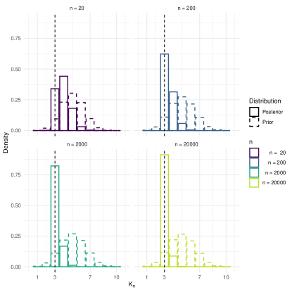
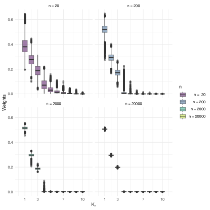
(a) $\bar{\alpha}_{n}:$ $\mathbb{E}[K_{n}]=5$	(b) $\bar{\alpha}_{n}:$ $\mathbb{E}[K_{n}]=5$
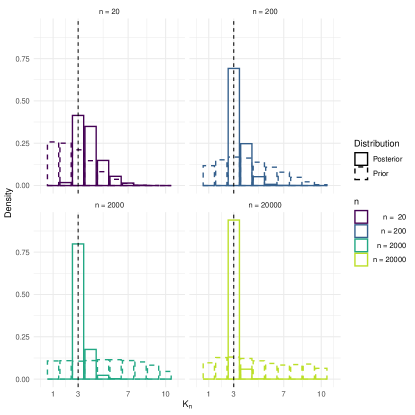
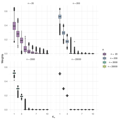
(c) $\bar{\alpha}\sim\text{Ga}(a,bK)$	(d) $\bar{\alpha}\sim\text{Ga}(a,bK)$

Figure 7: Dirichlet multinomial process mixtures varying concentration parameter $\bar{\alpha}$. (a) and (b): $\bar{\alpha}$ chosen such that $\mathbb{E}[K_{n}]=5$ for various choices of $n$. (c) and (d): a $\text{Ga}(a,bK)$ prior is used on $\bar{\alpha}$. (a) and (c): Prior and posterior distributions of the number of clusters $K_{n}$. (b) and (d): Boxplots of mixture weights.

We illustrate two different cases where the parameter $\bar{\alpha}$ is not fixed. First, we consider the fixed prior expected number of clusters, such as $\mathbb{E}[K_{n}]=5$, which leads to decreasing of the parameter $\bar{\alpha}$ with $n$. Posterior distribution of the number of clusters is presented in Figure 7 (a). We can see that the posterior concentrates at a correct number of clusters for different values of $n$. This observation is consistent with the posterior distribution of the weights at Figure 7 (b). Although we can not directly compare our experimental results with results obtained by Ohn and Lin (2022) due to different theoretical assumptions, we can note that theoretical results obtained by Ohn and Lin (2022) requires that $\bar{\alpha}$ decreases as $n^{-a_{0}}$, where $a_{0}>0$, which is faster than the $1/\log{n}$ decrease induced by fixing the expectation. So the obtained results suggest that the slower decrease rate for $\alpha$ might be enough to obtain consistency.

The second approach consists in using the hyperprior for parameter $\bar{\alpha}$. We consider $\bar{\alpha}\sim\text{Ga}(a,bK)$, where parameters $a=1$, $b=0.1$ and $K=10$ is the number of components, which leads to less informative prior distribution of the number of clusters. This simulation setting is also different from theoretical assumptions required by Ascolani et al. (2022). However, we can note that in this case posterior distribution also seems to concentrate at the $K_{0}$=3. Obtained results suggest the potential wider applicability of these two approaches then proven in Ohn and Lin (2022); Ascolani et al. (2022).

References

- Arbel and Favaro (2021) Arbel, J. and Favaro, S. (2021). “Approximating predictive probabilities of Gibbs-type priors.” Sankhya A, 83(1), 496–519.
- Argiento and De Iorio (2022) Argiento, R. and De Iorio, M. (2022). “Is infinity that far? A Bayesian nonparametric perspective of finite mixture models.” The Annals of Statistics.
- Ascolani et al. (2022) Ascolani, F., Lijoi, A., Rebaudo, G., and Zanella, G. (2022). “Clustering consistency with Dirichlet process mixtures.” Biometrika. In press.
- Attorre et al. (2020) Attorre, F., Cambria, V. E., Agrillo, E., Alessi, N., Alfò, M., De Sanctis, M., Malatesta, L., Sitzia, T., Guarino, R., Marcenò, C., et al. (2020). “Finite Mixture Model-based classification of a complex vegetation system.” Vegetation Classification and Survey, 1, 77.
- Bystrova et al. (2021) Bystrova, D., Arbel, J., Kon Kam King, G., and Deslandes, F. (2021). “Approximating the clusters’ prior distribution in Bayesian nonparametric models.” In Third Symposium on Advances in Approximate Bayesian Inference.
- Cai et al. (2021) Cai, D., Campbell, T., and Broderick, T. (2021). “Finite mixture models do not reliably learn the number of components.” In International Conference on Machine Learning, 1158–1169. PMLR.
- Carlton (2002) Carlton, M. A. (2002). “A family of densities derived from the three-parameter Dirichlet process.” Journal of applied probability, 39(4), 764–774.
- Celeux et al. (2000) Celeux, G., Hurn, M., and Robert, C. P. (2000). “Computational and inferential difficulties with mixture posterior distributions.” Journal of the American Statistical Association, 95(451), 957–970.
- Chambaz and Rousseau (2008) Chambaz, A. and Rousseau, J. (2008). “Bounds for Bayesian order identification with application to mixtures.” The Annals of Statistics, 36(2), 938–962.
- De Blasi et al. (2015) De Blasi, P., Favaro, S., Lijoi, A., Mena, R. H., Pruenster, I., and Ruggiero, M. (2015). “Are Gibbs-type priors the most natural generalization of the Dirichlet process?” IEEE Transactions on Pattern Analysis and Machine Intelligence, 37(2), 212–229.
- Ferguson (1973) Ferguson, T. (1973). “A Bayesian analysis of some nonparametric problems.” The Annals of Statistics, 1(2), 209–230.
- Fraley and Raftery (2002) Fraley, C. and Raftery, A. E. (2002). “Model-Based Clustering, Discriminant Analysis, and Density Estimation.” Journal of the American Statistical Association, 97(458), 611–631.
- Frühwirth-Schnatter (2006) Frühwirth-Schnatter, S. (2006). Finite mixture and Markov switching models, volume 425. Springer.
- Frühwirth-Schnatter et al. (2021) Frühwirth-Schnatter, S., Malsiner-Walli, G., and Grün, B. (2021). “Generalized Mixtures of Finite Mixtures and Telescoping Sampling.” Bayesian Analysis, 16(4), 1279 – 1307.
- Frühwirth-Schnatter et al. (2012) Frühwirth-Schnatter, S., Pamminger, C., Weber, A., and Winter-Ebmer, R. (2012). “Labor market entry and earnings dynamics: Bayesian inference using mixtures-of-experts Markov chain clustering.” Journal of Applied Econometrics, 27(7), 1116–1137.
- Frühwirth-Schnatter et al. (2019) Frühwirth-Schnatter, S., Celeux, G., and Robert, C. P. (eds.) (2019). Handbook of Mixture Analysis. CRC Press, Taylor & Francis Group.
- Gelman and Rubin (1992) Gelman, A. and Rubin, D. B. (1992). “Inference from iterative simulation using multiple sequences.” Statistical Science, 7(4), 457–472.
- Ghosal et al. (1999) Ghosal, S., Ghosh, J. K., and Ramamoorthi, R. V. (1999). “Posterior consistency of Dirichlet mixtures in density estimation.” The Annals of Statistics, 27(1), 143 – 158.
- Ghosal and Van Der Vaart (2007) Ghosal, S. and Van Der Vaart, A. (2007). “Posterior convergence rates of Dirichlet mixtures at smooth densities.” The Annals of Statistics, 35(2), 697–723.
- Ghosal and Van der Vaart (2017) Ghosal, S. and Van der Vaart, A. (2017). Fundamentals of nonparametric Bayesian inference, volume 44. Cambridge University Press.
- Gnedin and Pitman (2006) Gnedin, A. and Pitman, J. (2006). “Exchangeable Gibbs partitions and Stirling triangles.” Journal of Mathematical Sciences, 138(3), 5674–5685.
- Greve et al. (2022) Greve, J., Grün, B., Malsiner-Walli, G., and Frühwirth-Schnatter, S. (2022). “Spying on the prior of the number of data clusters and the partition distribution in Bayesian cluster analysis.” Australian & New Zealand Journal of Statistics, 64(2), 205–229.
- Guha et al. (2021) Guha, A., Ho, N., and Nguyen, X. (2021). “On posterior contraction of parameters and interpretability in Bayesian mixture modeling.” Bernoulli, 27(4), 2159–2188.
- Ho and Nguyen (2016) Ho, N. and Nguyen, X. (2016). “On strong identifiability and convergence rates of parameter estimation in finite mixtures.” Electronic Journal of Statistics, 10(1), 271–307.
- Ishwaran and Zarepour (2000) Ishwaran, H. and Zarepour, M. (2000). “Markov chain Monte Carlo in approximate Dirichlet and beta two-parameter process hierarchical models.” Biometrika, 87(2), 371–390.
- Ishwaran and Zarepour (2002) — (2002). “Exact and approximate sum representations for the Dirichlet process.” Canadian Journal of Statistics, 30(2), 269–283.
- James et al. (2009) James, L. F., Lijoi, A., and Prünster, I. (2009). “Posterior analysis for normalized random measures with independent increments.” Scandinavian Journal of Statistics, 36(1), 76–97.
- Kruijer et al. (2010) Kruijer, W., Rousseau, J., and Vaart, A. v. d. (2010). “Adaptive Bayesian density estimation with location-scale mixtures.” Electronic Journal of Statistics, 4(none), 1225–1257.
- Lijoi et al. (2020a) Lijoi, A., Prünster, I., and Rigon, T. (2020a). “Finite-dimensional discrete random structures and Bayesian clustering.” Preprint.
- Lijoi et al. (2020b) — (2020b). “The Pitman–Yor multinomial process for mixture modelling.” Biometrika, 107(4), 891–906.
- Lijoi et al. (2005) Lijoi, A., Prünster, I., and Walker, S. G. (2005). “On consistency of nonparametric normal mixtures for Bayesian density estimation.” Journal of the American Statistical Association, 100(472), 1292–1296.
- Lo (1984) Lo, A. Y. (1984). “On a class of Bayesian nonparametric estimates: I. Density estimates.” The Annals of Statistics, 351–357.
- Malsiner-Walli et al. (2016) Malsiner-Walli, G., Frühwirth-Schnatter, S., and Grün, B. (2016). “Model-based clustering based on sparse finite Gaussian mixtures.” Statistics and Computing, 26(1-2), 303–324.
- Miller (2022) Miller, J. W. (2022). “Consistency of mixture models with a prior on the number of components.”
- Miller and Dunson (2019) Miller, J. W. and Dunson, D. B. (2019). “Robust Bayesian Inference via Coarsening.” Journal of the American Statistical Association, 114(527), 1113–1125.