$p$-adic Cellular Neural Networks: Applications to Image Processing

Abstract.

The $p$-adic cellular neural networks (CNNs) are mathematical generalizations of the neural networks introduced by Chua and Yang in the 80s. In this work we present two new types of CNNs that can perform computations with real data, and whose dynamics can be understood almost completely. The first type of networks are edge detectors for grayscale images. The stationary states of these networks are organized hierarchically in a lattice structure. The dynamics of any of these networks consists of transitions toward some minimal state in the lattice. The second type is a new class of reaction-diffusion networks. We investigate the stability of these networks and show that they can be used as filters to reduce noise, preserving the edges, in grayscale images polluted with additive Gaussian noise. The networks introduced here were found experimentally. They are abstract evolution equations on spaces of real-valued functions defined in the $p$-adic unit ball for some prime number $p$. In practical applications the prime $p$ is determined by the size of image, and thus, only small primes are used. We provide several numerical simulations showing how these networks work.

1. Introduction

In the late 80s Chua and Yang introduced a new natural computing paradigm called the cellular neural networks (or cellular nonlinear networks) CNN which includes the cellular automata as a particular case [10], [11], [13]. This paradigm has been extremely successful in various applications in vision, robotics and remote sensing, see, e.g., [12], [32] and the references therein.

In [37] we introduce the $p$-adic cellular neural networks which are mathematical generalizations of the classical CNNs. The new networks have infinitely many cells which are organized hierarchically in rooted trees, and also they have infinitely many hidden layers. Intuitively, the $p$-adic CNNs occur as limits of large hierarchical discrete CNNs. A $p$-adic CNN is the dynamical system given by

$$\left\{\begin{array}[c]{l}\frac{\partial X(x,t)}{\partial t}=-X(x,t)+{\displaystyle\int\limits_{\mathbb{Q}_{p}}}A(x,y)Y(y,t)dy+{\displaystyle\int\limits_{\mathbb{Q}_{p}}}B(x,y)U(y)dy+Z(x)\\ \\ Y(x,t)=f(X(x,t)),\end{array}\right.$$ (1.1)

where $x$ is a $p$-adic number ($x\in\mathbb{Q}_{p}$), while $t$ is a non-negative real number, $X(x,t)\in\mathbb{R}$ is the state of cell $x$ at the time $t$, $Y(x,t)\in\mathbb{R}$ is the output of cell $x$ at the time $t$, $f$ is a sigmoidal nonlinearity, $U$ is the input of the CNN, and $Z$ is the threshold of the CNN. In [37], we study the Cauchy problem associated to (1.1) and also provide numerical methods for solving it.

The goal of this article is to show that $p$-adic CNNs can perform computations using real data, and that the dynamics can be understood almost completely. We present two new types of $p$-adic CNNs, one type for edge detection of grayscale images, and the other, for denoising of grayscale images polluted with Gaussian noise. It is important to emphasize that our goal is not to produce new techniques for image processing, but to use these tasks to verify that $p$-adic CNNs can perform relevant computations. On the other hand, classical CNNs have been implemented in hardware for performing certain image processing tasks. We have used some of the ideas introduced in [12], but our results go in a completely new direction.

We found experimentally that $p$-adic CNNs of the form

$$\left\{\begin{array}[c]{ll}\frac{\partial}{\partial t}X(x,t)=-X(x,t)+aY(x,t)+(B\ast U)(x)+Z(x),&x\in\mathbb{Z}_{p},t\geq 0;\\ &\\ Y(x,t)=f(X(x,t)),&\end{array}\right.$$ (1.2)

can be used as edge detectors, here $\mathbb{Z}_{p}$ is the $p$-adic unit ball, and $U$ is an image. We develop numerical algorithms for solving the Cauchy problem attached to (1.2), with initial datum $X(x,0)=0$. The simulations show that after a time sufficiently large the network outputs a black-and-white image approximating the edges of the original image $U(x)$. The performance of this edge detector is comparable to the Canny detector, and other well-known detectors. But most importantly, we can explain, reasonably well, how the network detects the edges of an image.

We determine all the stationary states of (1.2), i.e. the solutions of $\frac{\partial}{\partial t}X(x,t)=0$, for any $a\in\mathbb{R}$, see Lemma 1 and Theorem 1. We show that for $a>1$, the set of all possible stationary states $\mathcal{M}$ of (1.2) has a hierarchical structure, more precisely, $\left(\mathcal{M},\preccurlyeq\right)$ is a lattice, where $\preccurlyeq$ is a partial order. Furthermore, we determine the set of minimal elements of $\left(\mathcal{M},\preccurlyeq\right)$, see Theorem 2. The dynamics of the network consists of transitions in a hierarchically organized landscape $\left(\mathcal{M},\preccurlyeq\right)$ toward some minimal state. This is a reformulation of the classical paradigm asserting that the dynamics of a large class of complex systems can be modeled as a random walk on its energy landscape, see, e.g., [22], [23].

We found experimentally that $p$-adic CNNs of the form

$$\frac{\partial X(x,t)}{\partial t}=\mu X(x,t)+(\lambda I-\boldsymbol{D}_{0}^{\alpha})X(x,t)+{\displaystyle\int\limits_{\mathbb{Z}_{p}}}A(x-y)f(X(y,t))dy$$ (1.3)

$$+{\displaystyle\int\limits_{\mathbb{Z}_{p}}}B(x-y)U(y)dy+Z(x)$$

can be used for denoising grayscale images polluted with Gaussian noise. In this case, $X(x,0)$ is the input image, and $X(x,t_{0})$ is the output image, for a suitable (typically small) $t_{0}$.

The CNN (1.3) is a reaction-diffusion network. The diffusion part corresponds to

$$\frac{\partial X(x,t)}{\partial t}=(\lambda I-\boldsymbol{D}_{0}^{\alpha})X(x,t)\text{, }x\in\mathbb{Z}_{p},t\geq 0,$$ (1.4)

here $\boldsymbol{D}_{0}^{\alpha}$ is the Vladimirov operator acting on functions supported in the unit ball, $\alpha>0$. The equation (1.4) is a $p$-adic heat equation in the unit ball, this means that there is a stochastic Markov process attached to it. The paths of this stochastic process are discontinuous. $p$-Adic heat equations and the associated stochastic processes have been studied intensively in the last thirty years in connection with models of complex systems, see, e.g., [3]-[4], [14], [22], [25]-[23], [34]-[36], [38]-[39].

The reaction term in (1.3) gives an estimation of the edges of the image, while the diffusion term produces a smoothed version of the image. Under suitable hypotheses, see Theorem 3, we show that a solution of the initial value problem attached to (1.3) is bounded at very time if $\mu\leq 0$, otherwise, the solution is bounded by $Ce^{\mu t}$, where $C$ is a positive constant. Some numerical simulations show that our filter effectively reduces the noise while preserves the edges of the image, however, its performance is inferior to the Perona-Malik filter, see, e.g., [31].

Finally, we want to mention that $p$-adic numbers have been used before in processing image algorithms, see, e.g., [5]-[6], [26]. But these results are not directly related with the ones presented here.

2. Basic facts on $p$-adic analysis

In this section we fix the notation and collect some basic results about $p$-adic analysis that we will use through the article. For a detailed exposition on $p$-adic analysis the reader may consult [1], [33], [36]. For a quick review of $p$-adic analysis the reader may consult [7], [27].

2.1. The field of $p$-adic numbers

Throughout this article $p$ will denote a prime number. The field of $p-$adic numbers $\mathbb{Q}_{p}$ is defined as the completion of the field of rational numbers $\mathbb{Q}$ with respect to the $p-$adic norm $|\cdot|_{p}$, which is defined as

$$|x|_{p}=\begin{cases}0&\text{if }x=0\\ p^{-\gamma}&\text{if }x=p^{\gamma}\dfrac{a}{b},\end{cases}$$

where $a$ and $b$ are integers coprime with $p$. The integer $\gamma=ord_{p}(x)$ with $ord_{p}(0):=+\infty$, is called the $p-$adic order of $x$. The metric space $\left(\mathbb{Q}_{p},\left|\cdot\right|_{p}\right)$ is a complete ultrametric space. Ultrametric means that $\left|x+y\right|_{p}\leq\max\left\{\left|x\right|_{p},\left|y\right|_{p}\right\}$. As a topological space $\mathbb{Q}_{p}$ is homeomorphic to a Cantor-like subset of the real line, see, e.g., [1], [36].

Any $p-$adic number $x\neq 0$ has a unique expansion of the form

$$x=p^{ord_{p}(x)}\sum_{j=0}^{\infty}x_{j}p^{j},$$ (2.1)

where $x_{j}\in\{0,1,2,\dots,p-1\}$ and $x_{0}\neq 0$. It follows from (2.1), that any $x\in\mathbb{Q}_{p}\smallsetminus\left\{0\right\}$ can be represented uniquely as $x=p^{ord_{p}(x)}u\left(x\right)$ and $\left|x\right|_{p}=p^{-ord_{p}(x)}$.

2.2. Topology of $\mathbb{Q}_{p}$

For $r\in\mathbb{Z}$, denote by $B_{r}(a)=\{x\in\mathbb{Q}_{p};\left|x-a\right|_{p}\leq p^{r}\}$ the ball of radius $p^{r}$ with center at $a\in\mathbb{Q}_{p}$, and take $B_{r}(0):=B_{r}$. The ball $B_{0}$ equals the ring of $p-$adic integers $\mathbb{Z}_{p}$. We also denote by $S_{r}(a)=\{x\in\mathbb{Q}_{p};\left|x-a\right|_{p}=p^{r}\}$ the sphere of radius $p^{r}$ with center at $a\in\mathbb{Q}_{p}$, and take $S_{r}(0):=S_{r}$. We notice that $S_{0}=\mathbb{Z}_{p}^{\times}$ (the group of units of $\mathbb{Z}_{p}$). The balls and spheres are both open and closed subsets in $\mathbb{Q}_{p}$. In addition, two balls in $\mathbb{Q}_{p}$ are either disjoint or one is contained in the other.

As a topological space $\left(\mathbb{Q}_{p},\left|\cdot\right|_{p}\right)$ is totally disconnected, i.e. the only connected  subsets of $\mathbb{Q}_{p}$ are the empty set and the points. A subset of $\mathbb{Q}_{p}$ is compact if and only if it is closed and bounded in $\mathbb{Q}_{p}$, see e.g. [36, Section 1.3], or [1, Section 1.8]. The balls and spheres are compact subsets. Thus $\left(\mathbb{Q}_{p},\left|\cdot\right|_{p}\right)$ is a locally compact topological space.

Since $(\mathbb{Q}_{p},+)$ is a locally compact topological group, there exists a Haar measure $dx$, which is invariant under translations, i.e. $d(x+a)=dx$. If we normalize this measure by the condition $\int_{\mathbb{Z}_{p}}dx=1$, then $dx$ is unique. For a quick review of the integration in the $p$-adic framework the reader may consult [7], [27] and the references therein.

Notation 1.

We will use $\Omega\left(p^{-r}\left|x-a\right|_{p}\right)$ to denote the characteristic function of the ball $B_{r}(a)$.

2.3. The Bruhat-Schwartz space

A real-valued function $\varphi$ defined on $\mathbb{Q}_{p}$ is called locally constant if for any $x\in\mathbb{Q}_{p}$ there exist an integer $l(x)\in\mathbb{Z}$ such that

$$\varphi(x+x^{\prime})=\varphi(x)\text{ for any }x^{\prime}\in B_{l(x)}.$$ (2.2)

A function $\varphi:\mathbb{Q}_{p}\rightarrow\mathbb{C}$ is called a Bruhat-Schwartz function (or a test function) if it is locally constant with compact support. Any test function can be represented as a linear combination, with real coefficients, of characteristic functions of balls. The $\mathbb{R}$-vector space of Bruhat-Schwartz functions is denoted by $\mathcal{D}(\mathbb{Q}_{p})$. For $\varphi\in\mathcal{D}(\mathbb{Q}_{p})$, the largest number $l=l(\varphi)$ satisfying (2.2) is called the exponent of local constancy (or the parameter of constancy) of $\varphi$. Let $U$ be an open subset of $\mathbb{Q}_{p}$, we denote by $\mathcal{D}(U)$ the $\mathbb{R}$-vector space of all test functions with support in $U$. For instance $\mathcal{D}(\mathbb{Z}_{p})$ is the $\mathbb{R}$-vector space of all test functions with supported in   the unit ball $\mathbb{Z}_{p}$. A function $\varphi$ in $\mathcal{D}(\mathbb{Z}_{p})$ can be written as

$$\varphi\left(x\right)={\displaystyle\sum\limits_{j=1}^{M}}\varphi\left(\widetilde{x}_{j}\right)\Omega\left(p^{r_{j}}\left|x-\widetilde{x}_{j}\right|_{p}\right),$$

where the $\widetilde{x}_{j}$, $j=1,\ldots,M$, are points in $\mathbb{Z}_{p}$, the $r_{j}$, $j=1,\ldots,M$, are integers, and $\Omega\left(p^{r_{j}}\left|x-\widetilde{x}_{j}\right|_{p}\right)$ denotes the characteristic function of the ball $B_{-r_{j}}(\widetilde{x}_{j})=\widetilde{x}_{j}+p^{r_{j}}\mathbb{Z}_{p}$.

2.4. Some function spaces

Given $\rho\in[1,\infty)$, we denote by $L^{\rho}:=L^{\rho}\left(\mathbb{Z}_{p}\right):=L^{\rho}\left(\mathbb{Z}_{p},dx\right),$ the $\mathbb{R}-$vector space of all functions $g:\mathbb{Z}_{p}\rightarrow$ $\mathbb{R}$ satisfying

$$\left\|g\right\|_{\rho}=\left[{\textstyle\int\limits_{\mathbb{Z}_{p}}}\left|g\left(x\right)\right|^{\rho}dx\right]^{\frac{1}{\rho}}<\infty.$$

We denote by $\mathcal{C}(\mathbb{Z}_{p})$ the $\mathbb{R}$-vector space of continuous functions $f:\mathbb{Z}_{p}\rightarrow\mathbb{R}$ satisfying

$$\left\|f\right\|_{\infty}:=\max_{x\in\mathbb{Z}_{p}}\text{ }\left|f\left(x\right)\right|<\infty\text{.}$$ (2.3)

3. $p$-Adic continuous CNNs

3.1. A type $p$-adic continuous CNNs

In this section we present new edge detectors based on $p$-adic CNNs for grayscale images. We take $B\in L^{1}(\mathbb{Z}_{p})$ and $U,Z\in\mathcal{C}(\mathbb{Z}_{p})$, $a$, $b\in\mathbb{R}$ , and fix the sigmoidal function $f(s)=\frac{1}{2}(\left|s+1\right|-|s-1|)$ for $s\in\mathbb{R}$. In this section we consider the following $p$-adic CNN:

$$\left\{\begin{array}[c]{ll}\frac{\partial}{\partial t}X(x,t)=-X(x,t)+aY(x,t)+(B\ast U)(x)+Z(x),&x\in\mathbb{Z}_{p},t\geq 0;\\ &\\ Y(x,t)=f(X(x,t)).&\end{array}\right.$$ (3.1)

We denote this $p$-adic CNN as $CNN(a,B,U,Z)$, where $a,B,U,Z$ are the parameters of the network. In applications to edge detection, we take $U(x)$ to be a grayscale image, and take the initial datum as $X(x,0)=0$.

3.2. Stationary states

We say that $X_{stat}(x)$ is a stationary state of the network $CNN(a,B,U,Z)$, if

$$\left\{\begin{array}[c]{ll}X_{stat}(x)=aY_{stat}(x)+(B\ast U)(x)+Z(x),&x\in\mathbb{Z}_{p};\\ &\\ Y_{stat}(x)=f(X_{stat}(x)).&\end{array}\right.$$ (3.2)

Remark 1.

Let $\tilde{X}(x)$ be any solution of (3.2). Then

$$\widetilde{X}(x)=\left\{\begin{array}[c]{lcc}a+(B\ast U)(x)+Z(x)&\text{if}&\widetilde{X}(x)>1\\ -a+(B\ast U)(x)+Z(x)&\text{if}&\widetilde{X}(x)<-1,\end{array}\right.$$ (3.3)

and

$$\left(1-a\right)\widetilde{X}(x)=(B\ast U)(x)+Z(x)\text{ if }\left|\widetilde{X}(x)\right|\leq 1.$$ (3.4)

Lemma 1.

(i) If $a<1$, then the network $CNN(a,B,U,Z)$ has a unique stationary state $X_{stat}(x)\in\mathcal{C}(\mathbb{Z}_{p})$ given by

$$X_{stat}(x)=\left\{\begin{array}[c]{lcr}a+(B\ast U)(x)+Z(x)&\text{if}&(B\ast U)(x)+Z(x)>1-a\\ -a+(B\ast U)(x)+Z(x)&\text{if}&(B\ast U)(x)+Z(x)<-1+a\\ \frac{(B\ast U)(x)+Z(x)}{1-a}&\text{if}&|(B\ast U)(x)+Z(x)|\leq 1-a.\end{array}\right.$$ (3.5)

(ii) If $a=1$ , then the network $CNN(a,B,U,Z)$ has a unique stationary state $X_{stat}(x)\in L^{1}(\mathbb{Z}_{p})$ given by

$$X_{stat}(x)=\left\{\begin{array}[c]{lcr}1+(B\ast U)(x)+Z(x)&\text{if}&(B\ast U)(x)+Z(x)>0\\ -1+(B\ast U)(x)+Z(x)&\text{if}&(B\ast U)(x)+Z(x)<0\\ 0&\text{if}&(B\ast U)(x)+Z(x)=0.\end{array}\right.$$ (3.6)

Proof.

If $a<1$, it follows from (3.3)-(3.4) that (3.5) is a continuous stationary state since by the dominated convergence theorem $(B\ast U)(x)$ is continuous. To establish the uniqueness of the solution, let $X(x)\in\mathcal{C}(\mathbb{Z}_{p})$ be another stationary state. Consider a point $x_{0}\in\mathbb{Z}_{p}$ such that $X(x_{0})>1$. Then by (3.3), $X(x_{0})=a+(B\ast U)(x_{0})+Z(x_{0})>1$ consequently $(B\ast U)(x_{0})+Z(x_{0})>1-a$ and therefore

$$X(x_{0})=a+(B\ast U)(x_{0})+Z(x_{0}):=X_{stat}(x_{0}).$$

The cases $X(x_{0})<-1$ and $X\left|(x_{0})\right|<1$ are treated in a similar way.

The case $a=1$ follows from (3.4), in this case we have that $X_{stat}(x)\in L^{1}(\mathbb{Z}_{p})$ since $X_{stat}(x)$ is bounded. The continuity of $X_{stat}(x)$ requires further hypotheses on $B,U,Z$. ∎

Definition 1.

Assume that $a>1$. Given

$$I_{+}\subseteq\{x\in\mathbb{Z}_{p};\;1-a<(B\ast U)(x)+Z(x)\},$$

$$I_{-}\subseteq\{x\in\mathbb{Z}_{p};\;(B\ast U)(x)+Z(x)<a-1\},$$

satisfying $I_{+}\cap I_{-}=\varnothing$  and

$$\mathbb{Z}_{p}\smallsetminus\left(I_{+}\cup I_{-}\right)\subseteq\{x\in\mathbb{Z}_{p};\;1-a<(B\ast U)(x)+Z(x)<a-1\},$$

we define the function

$$X_{stat}(x;I_{+},I_{-})=\left\{\begin{array}[c]{lll}a+(B\ast U)(x)+Z(x)&\text{if}&x\in I_{+}\\ -a+(B\ast U)(x)+Z(x)&\text{if}&x\in I_{-}\\ \frac{(B\ast U)(x)+Z(x)}{1-a}&\text{if}&x\in\mathbb{Z}_{p}\setminus\left(I_{+}\cup I_{-}\right).\end{array}\right.$$ (3.7)

Theorem 1.

Assume that $a>1$. All functions of type (3.7) are stationary states of the network $CNN(a,B,U,Z)$. Conversely, any  stationary state of the network $CNN(a,B,U,Z)$ has the form (3.7).

Proof.

We first verify that any function of type (3.7) is a stationary state. Take a point $x_{0}\in\mathbb{Z}_{p}$. Since the sets $I_{+}$, $I_{-}$, $\mathbb{Z}_{p}\smallsetminus\left(I_{+}\cup I_{-}\right)$ are disjoint, three cases occur.

Case 1: $x_{0}\in I_{+}$.

If $x_{0}\in I_{+}$, then $X_{stat}(x_{0};I_{+},I_{-})=a+(B\ast U)(x_{0})+Z(x_{0})$ and by definition of $I_{+}$, $a+(B\ast U)(x_{0})+Z(x_{0})>1$. Then

$$af(X_{stat}(x_{0};I_{+},I_{-}))+(B\ast U)(x_{0})+Z(x_{0})=\\ a+(B\ast U)(x_{0})+Z(x_{0})=X_{stat}(x_{0};I_{+},I_{-}).$$

Case 2: $x_{0}\in I_{-}$.

If $x_{0}\in I_{-}$, then $X_{stat}(x_{0};I_{+},I_{-})=-a+(B\ast U)(x_{0})+Z(x_{0})$ and by definition of $I_{-}$, $-a+(B\ast U)(x_{0})+Z(x_{0})<-1$. Then

$$af(X_{stat}(x_{0};I_{+},I_{-}))+(B\ast U)(x_{0})+Z(x_{0})=\\ -a+(B\ast U)(x_{0})+Z(x_{0})=X_{stat}(x_{0};I_{+},I_{-}).$$

Case 3: $x_{0}\in\mathbb{Z}_{p}\smallsetminus\left(I_{+}\cup I_{-}\right)$.

If $x_{0}\notin I_{+}\sqcup I_{-}$, then $X_{stat}(x_{0};I_{+},I_{-})=\frac{(B\ast U)(x_{0})+Z(x_{0})}{1-a}$ and by definition of $\mathbb{Z}_{p}\smallsetminus\left(I_{+}\cup I_{-}\right)$, $-1\leq\frac{(B\ast U)(x_{0})+Z(x_{0})}{1-a}\leq 1$, then

$$af(X_{stat}(x_{0};I_{+},I_{-}))+(B\ast U)(x_{0})+Z(x_{0})=\\ a\frac{(B\ast U)(x_{0})+Z(x_{0})}{1-a}+(B\ast U)(x_{0})+Z(x_{0})=\frac{(B\ast U)(x_{0})+Z(x_{0})}{1-a}\\ =X_{stat}(x_{0};I_{+},I_{-}).$$

Therefore $X_{stat}(x_{0};I_{+},I_{-})$ is a stationary state of the network $CNN(a,B,U,Z)$.

Now, suppose that $X_{stat}(x)$ is a stationary state of network $CNN(a,B,U,Z)$. Set

$$I_{+}:=X_{stat}^{-1}((1,\infty))\text{, \ \ \ \ }I_{-}:=X_{stat}^{-1}((-\infty,-1)).$$

By using (3.3) and (3.4), we have

$$I_{+}\subseteq(B\ast U+Z)^{-1}((1-a,\infty)),$$

$$I_{-}\subseteq(B\ast U+Z)^{-1}((-\infty,a-1)),$$

and

$$\mathbb{Z}_{p}\smallsetminus\left(I_{+}\cup I_{-}\right)\subseteq(B\ast U+Z)^{-1}([1-a,a-1]).$$

Then $X_{stat}(x;I_{+},I_{-})$ is a well-defined function. Finally, using again (3.3) and (3.4), we conclude that $X_{stat}(x)=X_{stat}(x;I_{+},I_{-})$ for all $x\in\mathbb{Z}_{p}$. ∎

Remark 2.

Notice that

$$Y_{stat}(x;I_{+},I_{-}):=f\left(X_{stat}(x;I_{+},I_{-})\right)=\left\{\begin{array}[c]{lll}1&\text{if}&x\in I_{+}\\ -1&\text{if}&x\in I_{-}\\ \frac{(B\ast U)(x)+Z(x)}{1-a}&\text{if}&x\in\mathbb{Z}_{p}\setminus\left(I_{+}\cup I_{-}\right).\end{array}\right.$$

The function $Y_{stat}(x;I_{+},I_{-})$ is the output of the network. If $I_{+}\cup I_{-}=\mathbb{Z}_{p}$, we say that $X_{stat}(x;I_{+},I_{-})$ is bistable. The set $\mathcal{B}\left(I_{+},I_{-}\right)=\mathbb{Z}_{p}\setminus\left(I_{+}\cup I_{-}\right)$ measures how far $X_{stat}(x;I_{+},I_{-})$ is from being bistable. We call set $\mathcal{B}\left(I_{+},I_{-}\right)$ the set of bistability of $X_{stat}(x;I_{+},I_{-})$. If $\mathcal{B}\left(I_{+},I_{-}\right)=\varnothing$, then $X_{stat}(x;I_{+},I_{-})$ is bistable.

Remark 3.

If $I_{+}\cup I_{-}\subsetneqq\mathbb{Z}_{p}$, we say that $X_{stat}(x;I_{+},I_{-})$ is an unstable.

4. Hierarchical structure of the space of stationary states

A relation $\preccurlyeq$ is a partial order on a set $S$ if it satisfies: 1 (reflexivity) $f\preccurlyeq f$ for all $f$ in $S$; 2 (antisymmetry) $f\preccurlyeq g$ and $g\preccurlyeq f$ implies $f=g$; 3 (transitivity) $f\preccurlyeq g$ and $g\preccurlyeq h$ implies $f\preccurlyeq h$.  A partially ordered set $\left(S,\preccurlyeq\right)$ (or poset) is a set endowed with a partial order. A partially ordered set $\left(S,\preccurlyeq\right)$ is called a lattice if for every $f$, $g$ in $S$, the elements $f\wedge g=\inf\{f,g\}$ and $f\vee$ $g=\sup\{f,g\}$ exist. Here, $f\wedge g$ denotes the smallest element in $S$ satisfying $f\wedge g\preccurlyeq f$ and $f\wedge g\preccurlyeq g$; while $f\vee$ $g$  denotes the largest element in $S$ satisfying $f\preccurlyeq$ $f\vee$ $g$ and $g\preccurlyeq f\vee$ $g$. We say that $h\in S$ a minimal element of with respect to $\preccurlyeq$, if there is no element $f\in S$, $f\neq h$ such that $f\preccurlyeq h$.

Posets offer a natural way to formalize the notion of hierarchy.

We set

$$\mathcal{M}=\bigcup_{I_{+},I_{-}}\left\{X_{stat}(x;I_{+},I_{-})\right\},$$

where $I_{+},I_{-}$ run trough all the sets given in Definition 1.  Given $X_{stat}(x;I_{+},I_{-})$ and $X_{stat}(x;I_{+}^{\prime},I_{-}^{\prime})$ in $\mathcal{M}$, with $I_{+}\cup I_{-}\neq\mathbb{Z}_{p}$ or $I_{+}^{\prime}\cup I_{-}^{\prime}\neq\mathbb{Z}_{p}$, we define

$$X_{stat}(x;I_{+}^{\prime},I_{-}^{\prime})\preccurlyeq X_{stat}(x;I_{+},I_{-})\text{ if }I_{+}\cup I_{-}\subseteq I_{+}^{\prime}\cup I_{-}^{\prime}.$$ (4.1)

In the case $I_{+}\cup I_{-}=\mathbb{Z}_{p}$ and $I_{+}^{\prime}\cup I_{-}^{\prime}=\mathbb{Z}_{p}$, the corresponding stationary states $X_{stat}(x;I_{+},I_{-})$, $X_{stat}(x;I_{+},I_{-})$ are not comparable. Since the condition $I_{+}\cup I_{-}\subseteq I_{+}^{\prime}\cup I_{-}^{\prime}\$is equivalent to $\mathcal{B}\left(I_{+}^{\prime},I_{-}^{\prime}\right)=\mathbb{Z}_{p}\setminus(I_{1}^{\prime}\cup I_{-1}^{\prime})\subseteq\mathcal{B}\left(I_{1},I_{-1}\right)\mathcal{=}\mathbb{Z}_{p}\setminus(I_{1}\sqcup I_{-1})$, condition (4.1) means that the set of bistability of $X_{stat}(x;I_{+}^{\prime},I_{-}^{\prime})$ is smaller that the set of of bistability of $X_{stat}(x;I_{+},I_{-})$. Also, the condition $I_{+}\cup I_{-}\subseteq I_{+}^{\prime}\cup I_{-}^{\prime}$implies that

$$X_{stat}(x;I_{+}^{\prime},I_{-}^{\prime})(x)=X_{stat}(x;I_{+},I_{-})(x)\text{ for all }x\in I_{+}\cup I_{-}\cup\mathcal{B}\left(I_{+}^{\prime}\cup I_{-}^{\prime}\right).$$

By using this observation, one verifies that (4.1) defines a partial order in $\mathcal{M}$. This means that the set of stationary states of the network $CNN(a,B,U,Z)$, $a>1$, has a hierarchical structure, where the bistable stationary states are the minimal ones. Intuitively, the bistable stationary states are at the deepest level of $\mathcal{M}$. Furthermore, $\left(\mathcal{M},\preccurlyeq\right)$ is a lattice. Indeed, given $X_{stat}(x;I_{+}^{\prime},I_{-}^{\prime})$, $X_{stat}(x;I_{+},I_{-})$,in $\mathcal{M}$, it verifies that

$$X_{stat}(x;I_{+}^{\prime},I_{-}^{\prime})\wedge X_{stat}(x;I_{+},I_{-})=X_{stat}(x;I_{+}^{\prime\prime},I_{-}^{\prime\prime})\text{, }$$

where $I_{+}^{\prime\prime}=I_{+}\cup I_{+}^{\prime}$, $I_{-}^{\prime\prime}=I_{-}\cup I_{-}^{\prime}$, and

$$X_{stat}(x;I_{+}^{\prime},I_{-}^{\prime})\vee X_{stat}(x;I_{+},I_{-})=X_{stat}(x;I_{+}^{\prime\prime\prime},I_{-}^{\prime\prime\prime}),$$

where $I_{+}^{\prime\prime\prime}=I_{+}\cap I_{+}^{\prime}$, $I_{-}^{\prime\prime\prime}=I_{-}\cap I_{-}^{\prime}$. Therefore, we have established the following result:

Theorem 2.

$\left(\mathcal{M},\preccurlyeq\right)$ is a lattice. Furthermore, the set of minimal elements of $\left(\mathcal{M},\preccurlyeq\right)$ agrees with the set of bistable states of $CNN(a,B,U,Z)$.

5. Edge detection

5.1. A new class of edge detectors

We take $a>1$, $X(x,0)=0$, and $U(x)\in\mathcal{D}(\mathbb{Z}_{p})$ to be a grayscale image. We argue that network (3.1) works as an edge detector. By Theorem 1, network $CNN(a,B,U,Z)$, $a>1$ has steady states of the form

$$Y_{stat}(x)=f(X_{stat}\left(x\right))=\left\{\begin{array}[c]{lll}+1&\text{if}&(B\ast U)(x)+Z(x)>\text{Threshold}_{1}\\ -1&\text{if}&(B\ast U)(x)+Z(x)<\text{Threshold}_{2},\end{array}\right.$$ (5.1)

where Threshold₂, Threshold₁ are real numbers. This type of outputs occur for networks with stationary states where $I_{+}\sqcup I_{-}=\mathbb{Z}_{p}$. For instance, when $I_{+}\subseteq(B\ast U+Z)^{-1}((Threshold_{1},\infty))$ and $I_{-}\subseteq(B\ast U+Z)^{-1}((-\infty,Threshold_{2}))$. If $U(x)$ is sufficiently small, then $(B\ast U)(x)+Z(x)$ gives a measure of dispersion of the image intensities; if this value is larger than Threshold₁, the networks outputs $+1$ to indicate the existence of an edge, if value is smaller than Threshold₂, the network outputs $-1$ to indicate the nonexistence of an edge.

We conducted several numerical experiments with grayscale images. We implemented a numerical method for solving the initial value problem attached to network $CNN(a,B,U,Z)$, with $X(x,0)=0$ and $U(x)$ a grayscale image. The simulations show that after a sufficiently large time the network outputs a black-and-white image approximating the edges of the original image $U(x)$. This means that for $t$ sufficiently large $X(x,t)$ is close to a bistable stationary state $X_{stat}(x;I_{+},I_{-})$. Furthermore, after a certain sufficiently large time, the output of the network do not show a difference perceivable by the human eye. We interpret this result as the bistable stationary states are asymptotically stable; of course this is a mathematical conjecture.

We now give an intuitive picture of the dynamics of the network, for $t$ sufficiently large, using $\left(\mathcal{M},\preccurlyeq\right)$ as an asymptotic landscape for $CNN(a,B,U,Z)$. For $t$ sufficiently large, the network performs transitions between stationary states $X_{stat}(x;I_{+},I_{-})$ belonging to a small neighborhood $\mathcal{N}$ around a bistable state $X_{stat}^{\left(0\right)}(x;I_{+},I_{-})$, with $I_{+}\cup I_{-}=\mathbb{Z}_{p}$. The dynamics of the network consists of transitions in a hierarchically organized landscape $\left(\mathcal{M},\preccurlyeq\right)$ toward some minimal state. This is a reformulation of the classical paradigm asserting that the dynamics of a large class of complex systems can be modeled as a random walk on its energy landscape.

5.2. Discretization

To process an image $U(x)$, we use a discrete version of network $CNN(a,B,U,Z)$, $a>1$. In turn, this requires to determine suitable kernels $B(x)$. We address these matters on this section.

We take $L$  to be a positive integer, and set $G_{L}=\mathbb{Z}_{p}/p^{L}\mathbb{Z}_{p}$. We identify $i\in G_{L}$ with an element of the form

$$i=i_{0}+i_{1}p+\ldots+i_{L-1}p^{L-1},$$

where the $i_{k}$s belong to the set $\left\{0,1,\ldots,p-1\right\}$. We denote by $\mathcal{D}_{L}\left(\mathbb{Z}_{p}\right)$ the $\mathbb{R}$-vector space of test functions of the form

$$\varphi\left(x\right)={\displaystyle\sum\limits_{i\in G_{L}}}\varphi\left(i\right)\Omega\left(p^{L}\left|x-i\right|_{p}\right)$$

supported in the unit ball $\mathbb{Z}_{p}$. Since $\Omega\left(p^{L}\left|x-i\right|_{p}\right)\Omega\left(p^{L}\left|x-j\right|_{p}\right)=0$ for $i\neq j$, the set

$$\left\{\Omega\left(p^{L}\left|x-i\right|_{p}\right)\right\}_{i\in G_{L}}$$

is a basis of $\mathcal{D}_{L}\left(\mathbb{Z}_{p}\right)$. Notice that the dimension of $\mathcal{D}_{L}\left(\mathbb{Z}_{p}\right)$ is $p^{L}$.

Assuming that $B\left(x\right),U(x),Z(x)\in\mathcal{D}_{L}\left(\mathbb{Z}_{p}\right)$, the initial value problem

$$\left\{\begin{array}[c]{ll}\frac{\partial}{\partial t}X(x,t)=-X(x,t)+aY(x,t)+(B\ast U)(x)+Z(x),&x\in\mathbb{Z}_{p},t\geq 0;\\ &\\ X(x,0)=X_{0}\in\mathcal{D}_{L}\left(\mathbb{Z}_{p}\right).&\end{array}\right.$$ (5.2)

has unique solution

$$X(x,t)=\sum_{i\in G_{L}}X(i,t)\Omega\left(p^{L}\left|x-i\right|_{p}\right)$$ (5.3)

in $\mathcal{D}_{L}\left(\mathbb{Z}_{p}\right)$ for $t\geq 0$, see [37, Theorem 1].

This result allow us to obtain a discretization of (5.2) and (3.1) as follows. Take

$$U(x)=\sum_{i\in G_{L}}U(i)\Omega(p^{L}|x-i|),$$ (5.4)

$$Z(x)=\sum_{i\in G_{L}}Z(i)\Omega(p^{L}|x-i|),$$ (5.5)

and

$$B(x)=p^{M_{2}-M_{1}}\Omega(p^{M_{2}}|x|_{p})-\Omega(p^{M_{1}}|x|_{p})$$ (5.6)

for some integers $M_{1}\leq M_{2}\leq L$.

We now take $i$, $j\in G_{L}$ and an integer $M\leq L$, then

$$|i-j+p^{L}z|_{p}=|i-j|_{p}\text{ for any }z\in\mathbb{Z}_{p}.$$

By using this observation, one gets that

$$\Omega(p^{M}|x|_{p})\ast U(x)=$$ (5.7)

$$=\sum_{i\in G_{L}}\left\{\sum_{j\in G_{L}}U(j){\displaystyle\int\limits_{\mathbb{Z}_{p}}}\Omega(p^{M}|i-y|_{p})\Omega(p^{L}|y-j|_{p})dy\right\}\Omega(p^{L}|x-i|_{p})$$

$$=\sum_{i\in G_{L}}\left\{\sum_{j\in G_{L}}U(j){\displaystyle\int\limits_{j+p^{L}\mathbb{Z}_{p}}}\Omega(p^{M}|i-y|_{p})dy\right\}\Omega(p^{L}|x-i|_{p})$$

$$=\sum_{i\in G_{L}}\left\{p^{-L}\sum_{j\in G_{L}}U(j)\Omega(p^{M}|i-j|_{p})\right\}\Omega(p^{L}|x-i|_{p}).$$

Now, from (5.6)-(5.7), we get the following formula:

$$(B\ast U)(x)=$$ (5.8)

$$\sum_{i\in G_{l}}p^{-L}\left(p^{M_{2}-M_{1}}\sum_{j\in G_{l}}\Omega(p^{M_{2}}|i-j|_{p})U(j)-\sum_{j\in G_{l}}\Omega(p^{M_{1}}|i-j|_{p})U(j)\right)\Omega(p^{L}|x-i|_{p}).$$

We now replace (5.3)-(5.8) in the equation in (5.2) and use that $\{\Omega(p^{L}|x-i|)\}_{i\in G_{L}}$ is a basis of $\mathcal{D}_{L}(\mathbb{Z}_{p})$, to get  a discretization of (5.2):

$$\left\{\begin{array}[c]{ll}\frac{dX(i,t)}{dt}=-X(i,t)+aY(i,t)+p^{-L}\left(\mathcal{L}U\right)(i)+Z(i),&i\in G_{L}\\ X(i,0)=X_{0}(i),&\end{array}\right.$$ (5.9)

where

$$Y(i,t)=f\left(X(i,t)\right),\text{ }i\in G_{L},$$

and

$$\left(\mathcal{L}U\right)(i):=p^{M_{2}-M_{1}}\sum_{j\in G_{l}}\Omega(p^{M_{2}}|i-j|_{p})U(j)-\sum_{j\in G_{l}}\Omega(p^{M_{1}}|i-j|_{p})U(j),\text{ }i\in G_{L}.$$ (5.10)

5.2.1. Graph Laplacians

Let $G=(V,E)$ be a simple graph with vertices $V$ and edges $E$. Let $\phi:V\rightarrow\mathbb{R}$ be a function on the graph. The graph Laplacian $\Delta$ acting $\phi$ is defined as

$$\left(\Delta\phi\right)\left(v\right)={\displaystyle\sum\limits_{\begin{subarray}{c}w\in V\\ dist(w,v)=1\end{subarray}}}\left[\phi\left(v\right)-\phi\left(w\right)\right],$$

where $dist(w,v)$ is the distance on the graph. Now, let $N\left(v\right)$ be a fixed neighborhood of $v$, for instance,

$$\mathcal{N}\left(v\right)=\left\{w\in V;dist(w,v)\leq M\right\},$$

for positive integer $M$, a generalization of operator $\Delta$ is

$$\left(\Delta_{\mathcal{N}}\phi\right)\left(v\right)={\displaystyle\sum\limits_{w\in\mathcal{N}\left(v\right)}}\left(\Delta\phi\right)\left(w\right).$$ (5.11)

The operator $\mathcal{L}$ has the form (5.11). Indeed, the following formula holds for the operator $\left(\mathcal{L}U\right)(i)$:

$$\left(\mathcal{L}U\right)(i)=\sum_{\begin{subarray}{c}j\in G_{L}\\ |i-j|_{p}\leq p^{-M_{2}}\end{subarray}}\left[\sum_{\begin{subarray}{c}k\in G_{L}\\ p^{-M_{2}}<|j-k|_{p}\leq p^{-M_{1}}\end{subarray}}\left[U(j)-U(k)\right]\right]\text{, }i\in G_{L}\text{.}$$ (5.12)

In particular, taking $M_{1}=0$, $M_{2}=1$, one gets that

$$\sum_{\begin{subarray}{c}k\in G_{L}\\ p^{-1}<|j-k|_{p}\leq 1\end{subarray}}\left[U(j)-U(k)\right]=\sum_{\begin{subarray}{c}k\in G_{L}\\ |j-k|_{p}=1\end{subarray}}\left[U(j)-U(k)\right],$$

which is the graph Laplacian on $\ G_{L}=\mathbb{Z}_{p}/p^{L}\mathbb{Z}_{p}$ with the distance induced by $|\cdot|_{p}$.

Finally, we establish formula (5.12). We use that

$$\#\left\{k\in G_{L};p^{-M_{2}}<|j-k|_{p}\leq p^{-M_{1}}\right\}=p^{M_{2}-M_{1}},$$

since $i=i_{0}+i_{1}p+\ldots+i_{L-1}p^{L-1}$. Now $\left|i-j\right|_{p}\leq p^{-M_{2}}$ and $p^{-M_{2}}<|j-k|_{p}\leq p^{-M_{1}}$ imply that

$$\left|i-k\right|_{p}=\max\left\{\left|i-j\right|_{p},|j-k|_{p}\right\}=|j-k|_{p}\leq p^{-M_{1}},$$

by ultrametric property of $\left|\cdot\right|_{p}$. Then

$$\sum_{\begin{subarray}{c}j\in G_{L}\\ |i-j|_{p}\leq p^{-M_{2}}\end{subarray}}\left[\sum_{\begin{subarray}{c}k\in G_{L}\\ p^{-M_{2}}<|j-k|_{p}\leq p^{-M_{1}}\end{subarray}}\left[U(j)-U(k)\right]\right]=$$

$$\sum_{\begin{subarray}{c}j\in G_{L}\\ |i-j|_{p}\leq p^{-M_{2}}\end{subarray}}\left[\#\left\{k\in G_{L};p^{-M_{2}}<|j-k|_{p}\leq p^{-M_{1}}\right\}\right]U(j)$$

$$-\sum_{\begin{subarray}{c}j\in G_{L}\\ |i-j|_{p}\leq p^{-M_{2}}\end{subarray}}\text{ \ }\sum_{\begin{subarray}{c}k\in G_{L}\\ p^{-M_{2}}<|j-k|_{p}\leq p^{-M_{1}}\end{subarray}}U(k)=$$

$$\sum_{\begin{subarray}{c}j\in G_{L}\\ |i-j|_{p}\leq p^{-M_{2}}\end{subarray}}p^{M_{2}-M_{1}}U(j)-\sum_{\begin{subarray}{c}k\in G_{L}\\ |i-k|_{p}\leq p^{-M_{1}}\end{subarray}}U(k)=\left(\mathcal{L}U\right)(i).$$

6. Numerical Examples

To construct an edge detector using (5.9), it requires an algorithm for splitting a large image into smaller sub-images. Given an image $I$ of size $(n,m)$, a prime $p$ and an integer $K$, the algorithm divides image $I$ into sub-images $I_{r}^{\prime}$ of size $(p^{K},p^{K})$ or less. Then, we use another algorithm to codify sub-image $I_{r}^{\prime}$ as a test function $Test(I_{r}^{\prime})$. These algorithms are presented in the Appendix. We process the test function $Test(I_{r}^{\prime})=U$ using network

$$\left\{\begin{array}[c]{ll}\frac{dX(i,t)}{dt}=-X(i,t)+aY(i,t)+\sum_{j=0}^{8}\left\{U(i)-U(i+j3^{2})\right\}+z_{0},&i\in G_{L}\\ X(i,0)=0&\\ Y(i,t)=f(X(i,t)),&\end{array}\right.$$ (6.1)

with $p=3$, $L=4$, $M_{1}=2$, $M_{2}=4$, and $Z(i)=z_{0}\in\mathbb{R}$, for $i\in G_{L}$, and rescaling $\left(\mathcal{L}U\right)(i)$ as $3^{4}\left(\mathcal{L}U\right)(i)$, for $i\in G_{L}$, to get another test function $Y(i,t_{0};Test(I_{r}^{\prime}))$ taking values in $\left\{\pm 1\right\}$. Each test function $Y(i,t_{0};Test(I_{r}^{\prime}))$ is transformed into an image $I_{r}^{edges}$, at the final step, we concatenate all the images $I_{r}^{edges}$ to obtain a full image $I^{edges}$, which is the output  image. The time $t_{0}$ is chosen on a case-by-case basis so that the edges are as sharp as possible. See Figures 1, 2.

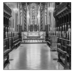
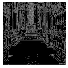
Figure 1. Left side, the original image. Right side, edges obtained by using a Canny edge detector.

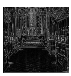
Figure 2. Left side, edges obtained by using CNN (6.1), with $z_{0}=-1$ and $6$ steps. Right side, edges obtained by using CNN (6.1), with $z_{0}=-1$ and $10$ steps.

7. Reaction-diffusion Cellular Neural Networks

7.1. The $p$-adic heat equation

For $\alpha>0$, the Vladimirov-Taibleson operator $\boldsymbol{D}^{\alpha}$ is defined as

$$\begin{array}[c]{ccc}\mathcal{D}(\mathbb{Q}_{p})&\rightarrow&L^{2}(\mathbb{Q}_{p})\cap\mathcal{C}\left(\mathbb{Q}_{p}\right)\\ &&\\ \varphi&\rightarrow&\boldsymbol{D}^{\alpha}\varphi,\end{array}$$

where

$$\left(\boldsymbol{D}^{\alpha}\varphi\right)\left(x\right)=\frac{1-p^{\alpha}}{1-p^{-\alpha-1}}{\displaystyle\int\limits_{\mathbb{Q}_{p}}}\frac{\left[\varphi\left(x-y\right)-\varphi\left(x\right)\right]}{\left|y\right|_{p}^{\alpha+1}}dy.$$

The $p$-adic analogue of the heat equation is

$$\frac{\partial u\left(x,t\right)}{\partial t}+a\boldsymbol{D}^{\alpha}u\left(x,t\right)=0\text{, with }a>0\text{.}$$

The solution of the Cauchy problem attached to the heat equation with initial datum $u\left(x,0\right)=\varphi\left(x\right)\in\mathcal{D}(\mathbb{Q}_{p})$ is given by

$$u\left(x,t\right)={\displaystyle\int\limits_{\mathbb{Q}_{p}}}Z\left(x-y,t\right)\varphi\left(y\right)dy,$$

where $Z\left(x,t\right)$ is the $p$-adic heat kernel defined as

$$Z\left(x,t\right)={\displaystyle\int\limits_{\mathbb{Q}_{p}}}\chi_{p}\left(-x\xi\right)e^{-at\left|\xi\right|_{p}^{\alpha}}d\xi,$$ (7.1)

where $\chi_{p}\left(-x\xi\right)$ is the standard additive character of the group $\left(\mathbb{Q}_{p},+\right)$. The $p$-adic heat kernel is the transition density function of a Markov stochastic process with space state $\mathbb{Q}_{p}$, see, e.g., [25], [39].

7.2. The $p$-adic heat equation on the unit ball

We define the operator $\boldsymbol{D}_{0}^{\alpha}$, $\alpha>0$, by restricting $\boldsymbol{D}^{\alpha}$ to $\mathcal{D}(\mathbb{Z}_{p})$ and considering $\left(\boldsymbol{D}^{\alpha}\varphi\right)\left(x\right)$ only for $x\in\mathbb{Z}_{p}$. The operator $\boldsymbol{D}_{0}^{\alpha}$ satisfies

$$\boldsymbol{D}_{0}^{\alpha}\varphi(x)=\lambda\varphi(x)+\frac{1-p^{\alpha}}{1-p^{-\alpha-1}}{\displaystyle\int\limits_{\mathbb{Z}_{p}}}\frac{\varphi(x-y)-\varphi(x)}{|y|_{p}^{\alpha+1}}dy,$$

for $\mathbb{\varphi\in}\mathcal{D}(\mathbb{Z}_{p})$, with $\lambda=\frac{p-1}{p^{\alpha+1}-1}p^{\alpha}$.

Consider the Cauchy problem

$$\left\{\begin{array}[c]{lll}\frac{\partial u\left(x,t\right)}{\partial t}+\boldsymbol{D}_{0}^{\alpha}u\left(x,t\right)-\lambda u\left(x,t\right)=0\text{, }&x\in\mathbb{Z}_{p},&t>0;\\ &&\\ u\left(x,0\right)=\varphi\left(x\right),&x\in\mathbb{Z}_{p},&\end{array}\right.$$

where $\mathbb{\varphi\in}\mathcal{D}(\mathbb{Z}_{p})$. The solution of this problem is given by

$$u\left(x,t\right)={\displaystyle\int\limits_{\mathbb{Z}_{p}}}Z_{0}(x-y,t)\varphi\left(y\right)dy\text{, }x\in\mathbb{Z}_{p}\text{, }t>0,$$

where

$$Z_{0}(x,t) :=e^{\lambda t}Z(x,t)+c(t)\text{, }x\in\mathbb{Z}_{p}\text{, }$$

$$c(t) :=1-(1-p^{-1})e^{\lambda t}\sum_{n=0}^{\infty}\frac{(-1)^{n}}{n!}t^{n}\frac{1}{1-p^{-n\alpha-1}}$$

and $Z(x,t)$ is given (7.1). The function $Z_{0}(x,t)$ is non-negative for $x\in\mathbb{Z}_{p}$, $t>0$, and

$${\displaystyle\int\limits_{\mathbb{Z}_{p}}}Z_{0}(x,t)dx=1,$$

[25]. Furthermore, $Z_{0}(x,t)$ is the transition density function of a Markov process with space state $\mathbb{Z}_{p}$.

The family

$$\begin{array}[c]{cccc}T_{t}:&L^{1}(\mathbb{Z}_{p})&\rightarrow&L^{1}(\mathbb{Z}_{p})\\ &&&\\ &\phi(x)&\rightarrow&T_{t}\phi(x):={\displaystyle\int\limits_{\mathbb{Z}_{p}}}Z_{0}(x-y,t)\phi(y)dy,\end{array}$$ (7.2)

is a $C^{0}$-semigroup of contractions with generator $\boldsymbol{D}_{0}^{\alpha}-\lambda I$ on $L^{1}(\mathbb{Z}_{p})$, see [20, Proposition 4, Proposition 5]

7.3. Reaction-diffusion CNNs

Definition 2.

Given $\mu\in\mathbb{R}$, $\alpha>0$, $A$, $B$,$U$, $Z\in\mathcal{C}(\mathbb{Z}_{p})$, a $p$-adic reaction-diffusion CNN, denoted as $CNN\left(\mu,\alpha,A,B,U,Z\right)$, is the dynamical system given by the following integro-differential equation:

$$\frac{\partial X(x,t)}{\partial t} =\mu X(x,t)+(\lambda I-\boldsymbol{D}_{0}^{\alpha})X(x,t)+{\displaystyle\int\limits_{\mathbb{Z}_{p}}}A(x-y)f(X(y,t))dy$$ (7.3)

$$+{\displaystyle\int\limits_{\mathbb{Z}_{p}}}B(x-y)U(y)dy+Z(x),$$

where $x\in\mathbb{Z}_{p}$, $t\geq 0$. We say that $X(x,t)\in$ $\mathbb{R}$ is the state of cell $x$ at the time $t$. Function $A$ is the kernel of the feedback operator, while function $B$ is the kernel of the feedforward operator. Function $U$ is the input of the CNN, while function $Z$ is the threshold of the CNN.

Notice that if $\mu=0$ and $A=B=U=Z=0$, (7.3) becomes the $p$-adic heat equation in the unit ball. Then, in (7.3), $(\lambda I-\boldsymbol{D}_{0}^{\alpha})$ is the diffusion term, while the other terms are the reaction ones, which describe the interaction between $X(x,t)$, $U(x)$, and $Z(x)$.

Remark 4.

In this section, we assume that $f$ is an arbitrary Lipschitz function, $f(0)=0$, i.e., $\left|f(s)-f(t)\right|\leq L(f)\left|s-t\right|$, for $s$, $t\in\mathbb{R}$, where $L(f)$ is a positive constant.

Lemma 2.

Let $A$, $B$, $U$, $Z\in\mathcal{C}(\mathbb{Z}_{p}).$

(i) Set

$$\boldsymbol{H}(g):={\displaystyle\int\limits_{\mathbb{Z}_{p}}}A(x-y)f\left(g(y)\right)dy+{\displaystyle\int\limits_{\mathbb{Z}_{p}}}B(x-y)U(y)dy+Z(x),$$ (7.4)

for $g\in L^{1}(\mathbb{Z}_{p})$. Then $\boldsymbol{H}:L^{1}(\mathbb{Z}_{p})\rightarrow L^{1}(\mathbb{Z}_{p})$ is a well-defined  operator satisfying

$$\|\boldsymbol{H}(g)-\boldsymbol{H}(g^{\prime})\|_{1}\leq L(f)\|A\|_{\infty}\|g-g^{\prime}\|_{1}\text{, for }g\text{, }g^{\prime}\in L^{1}(\mathbb{Z}_{p})\text{.}$$

(ii) The restriction of $\boldsymbol{H}$ to $\mathcal{C}(\mathbb{Z}_{p})$ satisfies

$$\|\boldsymbol{H}(g)-\boldsymbol{H}(g^{\prime})\|_{\infty}\leq L(f)\|A\|_{1}\|g-g^{\prime}\|_{\infty}\text{, for }g\text{, }g^{\prime}\in\boldsymbol{C}(\mathbb{Z}_{p})\text{,}$$

so $\boldsymbol{H}:\mathcal{C}(\mathbb{Z}_{p})\rightarrow\mathcal{C}(\mathbb{Z}_{p})$ is well-defined operator.

Proof.

Take $g,g^{\prime}\in L^{1}(\mathbb{Z}_{p})$, then

$$\|\boldsymbol{H}(g)-\boldsymbol{H}(g^{\prime})\|_{1}=\|{\displaystyle\int\limits_{\mathbb{Z}_{p}}}A(x-y)\left\{f\left(g(y)\right)-f\left(g^{\prime}(y)\right)\right\}dy\|_{1}$$

$$\leq{\displaystyle\int\limits_{\mathbb{Z}_{p}}}\left\{{\displaystyle\int\limits_{\mathbb{Z}_{p}}}\left|A(x-y)\right|\text{ }\left|f\left(g(y)\right)-f\left(g^{\prime}(y)\right)\right|dy\right\}dx\leq L(f)\|A\|_{\infty}{\displaystyle\int\limits_{\mathbb{Z}_{p}}}\left|g(y)-g^{\prime}(y)\right|dy$$

$$\leq L(f)\|A\|_{\infty}\|g-g^{\prime}\|_{1}.$$

This inequality also proves that $\boldsymbol{H}$ is well-defined. The second part is established in a similar way. ∎

Proposition 1.

Let $A$, $B$, $U$, $Z\in\mathcal{C}(\mathbb{Z}_{p})$. Take $X_{0}\in L^{1}(\mathbb{Z}_{p})$ as the initial datum for the Cauchy problem attached to (7.3). Then there exists $\tau=\tau\left(X_{0}\right)\in\left(0,\infty\right]$ and a unique $X(t)\in\mathcal{C}([0,\tau],L^{1}(\mathbb{Z}_{p}))$ satisfying

$$\left\{\begin{array}[c]{l}X(t)=e^{\mu t}T_{t}X_{0}+\int_{0}^{t}e^{\mu(t-s)}T_{t-s}\boldsymbol{H}(X(s))ds\\ X(0)=X_{0}.\end{array}\right.$$ (7.5)

Proof.

By [20, Proposition 4], $(\boldsymbol{D}_{0}^{\alpha}-\lambda I)$ is the generator of a strongly continuous semigroup $\left\{T_{t}\right\}_{t\geq 0}$ of contraction on $L^{1}(\mathbb{Z}_{p})$. Then $(\boldsymbol{D}_{0}^{\alpha}-\lambda I)+\mu I$ is the generator of a strongly continuous semigroup $\left\{e^{\mu t}T_{t}\right\}_{t\geq 0}$ on $L^{1}(\mathbb{Z}_{p})$, see [28, Theorem 4.3-(10)]. Since $\left\|e^{\mu t}T_{t}\right\|\leq e^{\mu t}$ and $\boldsymbol{H}$ is a Lipschitz nonlinearity, see Lemma 2-(i), there exits a unique  mild solution $X(t)\in\mathcal{C}([0,\tau],L^{1}(\mathbb{Z}_{p}))$ satisfying (7.5), see, e.g., [28, Theorem 5.1.2]. ∎

Lemma 3.

Let $A$, $B$, $U$, $Z\in\mathcal{C}(\mathbb{Z}_{p})$. Take $X_{0}\in\mathcal{C}(\mathbb{Z}_{p})$. Then, the integral equation (7.5) has unique solution $\mathcal{C}([0,\infty),\mathcal{C}(\mathbb{Z}_{p}))$.

Proof.

It is sufficient to show that (7.5) has a unique solution in $\mathcal{C}(\left[0,T\right],\mathcal{C}(\mathbb{Z}_{p}))$, where $T>0$ is an arbitrary time horizon. Indeed, if $X_{0}(t)\in\mathcal{C}(\left[0,T_{0}\right],\mathcal{C}(\mathbb{Z}_{p}))$ and $X_{1}(t)\in\mathcal{C}(\left[0,T_{1}\right],\mathcal{C}(\mathbb{Z}_{p}))$, with $T_{0}\leq T_{1}$, are mild solutions, then $X_{0}(t)=X_{1}(t)$ for $t\in\left[0,T_{1}\right]$, see [28, Theorem 5.2.3].

We set $\mathcal{Y}:=\mathcal{C}([0,T],\mathcal{C}(\mathbb{Z}_{p}))$, which is a Banach space with  norm

$$\sup_{0\leq t\leq T}\left\|Y\left(t\right)\right\|_{\infty}=\sup_{0\leq t\leq T}\left[\sup_{x\in\mathbb{Z}_{p}}\left|Y(x,t)\right|\right].$$

We now set

$$\boldsymbol{G}g(t):=e^{\mu t}T_{t}X_{0}+\int_{0}^{t}e^{\mu(t-s)}T_{t-s}\boldsymbol{H}\left(g(s)\right)ds,$$

for $g(t)\in\mathcal{C}([0,T],\mathcal{C}(\mathbb{Z}_{p}))$. By using that $Z_{0}(x,t)\in L^{1}(\mathbb{Z}_{p})$, one gets $T_{t}g\in\mathcal{C}([0,T],\mathcal{C}(\mathbb{Z}_{p}))$, and by Lemma 2-(ii), $\boldsymbol{G}:\mathcal{Y}\rightarrow\mathcal{Y}$. We now set

$$\boldsymbol{G}^{n}=\underbrace{\underset{n-times}{\boldsymbol{G}\circ\boldsymbol{G\circ\cdots\circ G}}}.$$

We show that for $n$ sufficiently large $\boldsymbol{G}^{n}$ is a contraction. We first notice that

$$\left\|\boldsymbol{G}g(t)-\boldsymbol{G}g(t)\right\|_{\infty}\leq L(f)e^{\mu T}\left\|A\right\|_{1}\|g(t)-g^{\prime}(t)\|_{\infty}.$$

By a well-known argument, see [28, Proof of Theorem 5.1.2], one gets that

$$\left\|\boldsymbol{G}^{n}g(t)-\boldsymbol{G}^{n}g(t)\right\|_{\infty}\leq\frac{(e^{\mu T}L(f)\|A\|_{1}T)^{n}}{n!}\|g(t)-g^{\prime}(t)\|_{\infty},$$

with $\frac{(e^{\mu T}L(f)\|A\|_{1}T)^{n}}{n!}<1$, for $n$ sufficiently large. Therefore $\boldsymbol{G}$ has a unique fixed point $X(t)$ in $\mathcal{Y}$, see [28, Theorem 1.1.3]. ∎

Theorem 3.

Let $X(t)\in\mathcal{C}([0,\infty),\mathcal{C}(\mathbb{Z}_{p}))$ be the unique solution of (7.5), with initial condition $X_{0}\in\mathcal{C}(\mathbb{Z}_{p})$.Then,

$$\|X(t)\|_{\infty}\leq e^{\mu t}\|X_{0}\|_{\infty}+\frac{(e^{\mu t}-1)}{\mu}\left(\|A\|_{1}\|f\|_{\infty}+\|B\|_{1}\|U\|_{\infty}+\|Z\|_{\infty}\right),$$ (7.6)

if $\mu\neq 0$, otherwise

$$\|X(t)\|_{\infty}\leq\|X_{0}\|_{\infty}+\tau\left(\|A\|_{1}\|f\|_{\infty}+\|B\|_{1}\|U\|_{\infty}+\|Z\|_{\infty}\right).$$ (7.7)

Proof.

By using that $\left\|B\ast U\right\|\leq\|B\|_{1}\|U\|_{\infty}$, cf. [33, Theorem 1.7], and Lemma 2-(ii), we get that

$$\|\boldsymbol{H}(g)\|_{\infty}\leq L(f)\|A\|_{1}\|g\|_{\infty}+\|B\|_{1}\|U\|_{\infty}+\|Z\|_{\infty}\text{ for }g,\in\boldsymbol{C}(\mathbb{Z}_{p}).$$

Now, the stated formula follows from (7.5), by Lemma 3,  by using that $\|A\|_{1}\leq\|A\|_{\infty}$ and $\|B\|_{1}\leq\|B\|_{\infty}$. The bound (7.7) is established in a similar way. ∎

8. Denoising

In this section, we present a new denoising technique based on certain reaction-diffusion CNNs. We first consider the initial value problem

$$\left\{\begin{array}[c]{lll}\frac{\partial X(x,t)}{\partial t}+\boldsymbol{D}_{0}^{1}X(x,t)-\lambda X(x,t)=0,&x\in\mathbb{Z}_{p},&t>0\\ &&\\ X(x,0)=X_{0}(x),&x\in\mathbb{Z}_{p},&\end{array}\right.$$ (8.1)

where $X_{0}(x)\in$ $[0,1]$ is a grayscale image codified as a test function supported in the unit ball $\mathbb{Z}_{p}$. The algorithm for this coding is discussed at the end of this section. The output image $X(x,t)$ is similar to the one produced by the classical Gaussian filter. See Figure 3.

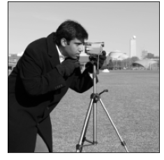
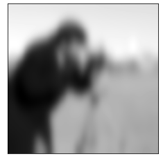
Figure 3. On the left side, the original image $X(x,0)$. On the right side $X(x,3)$.

In this article we propose the following reaction-diffusion CNN for denoising grayscale images polluted with normal additive noise:

$$\frac{\partial X(x,t)}{\partial t}=3X(x,t)+(\lambda I-\boldsymbol{D}_{0}^{\alpha})X(x,t)+3B\ast\left[X_{0}(x)-f(X(x,t))\right],$$ (8.2)

where $\alpha=0.75$, $f(x)=0.5(|x+1|-|x-1|)$, $B(x)=(\Omega(p^{2}|x|_{p})-\Omega(|x|_{p}))$, and $-1\leq X_{0}(x)\leq 1$. Notice that we are using the interval $\left[-1,1\right]$ as a grayscale scale. This equation was found experimentally. Natively, the reaction term $3X(x,t)+3B\ast\left[X_{0}(x)-f(X(x,t))\right]$ gives an estimation of the edges of the image, while the diffusion term $(\lambda I-\boldsymbol{D}_{0}^{\alpha})X(x,t)$ produces a smoothed version of the image.

The processing of an image $X_{0}(x)$ using (6.1) requires solving the corresponding Cauchy problem with initial datum $X(x,0)=X_{0}(x)$. Given an image $I$, i.e., a matrix of size $\left(n,m\right)$, and a pixel $(i,j)$ of $I$ , for the processing of this pixel we use a neighborhood $I_{i,j}$ centered at this pixel, which is sub-image $I_{i,j}$ of size $\left(p^{K},p^{K}\right)$, where $p^{2K}$ is the number of pixels in the sub-image $I_{i,j}$. We use small primes, $p=2,3$ to get sub-images of size $2\times 2$ and $3\times 3$. The choosing of the prime $p$ is completely determined by the image size, then, only small primes are required. Now, we codify the sub-image $I_{i,j}$ a test function $Test(I_{i,j})$ and solve numerically the Cauchy problem attached to (6.1) with initial datum $Test(I_{i,j})$. We pick a time $t_{0}$, on a case by case basis, and take the test function $X(x,t_{0};I_{i,j})$ as the output of the network. At the final step, we transform $X(x,t_{0};I_{i,j})$ into an image $I_{i,j}^{\prime},$ and take the pixel processed image at $(i,j)$ as the center of $I_{i,j}^{\prime}$. See Figures 4, 5.

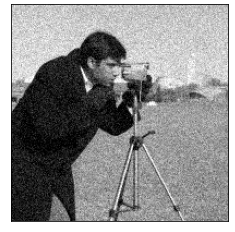
Figure 4. Left side, the original image. Right side, the image plus Gaussian noise, mean zero and variance $0.05$.

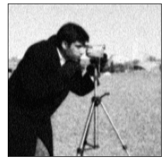
Figure 5. Left side, filtered image using Equation 8.2. Right side, filtered image obtained by using Perona-Malik equation with $\lambda=0.04$, $\delta_{t}=0.075$, and  $t=100$ iterations, and $g_{1}(s)$, see [8].

9. Appendix: Images and test functions

In this appendix. we show the existence of a bijective correspondence between images and test functions. We first show the existence of a bijective correspondence between finite disjoint unions of balls contained in $\mathbb{Z}_{p}$, for some prime $p$ with weighted rooted trees of valence $p$. The connections between clustering, trees and ultrametric spaces are well-known, see e.g., [22, Chapter 2] and the references therein. Finally, we show the existence of a bijective correspondence between finite, regular rooted trees of valence $p$ with images.

9.1. Finite rooted trees and test functions

By a finite rooted tree $\mathcal{T}$, we mean a finite undirected graph in which any two vertices are connected by  exactly one path. The vertices $V(\mathcal{T})$ of $\mathcal{T}$ are organized in disjoint levels:

$$V(\mathcal{T})={\textstyle\bigsqcup\limits_{j=0}^{M}}Level_{j}\left(\mathcal{T}\right),$$

where $Level_{j}\left(\mathcal{T}\right):=Level_{j}=\left\{v_{j,0},v_{j,1},\ldots,v_{j,k_{j}}\right\}$, $k_{j}\geq 1$, are the vertices of $\mathcal{T}$ at level $j$. At level $0$ there is exactly one vertex $v_{0}$, the root of the tree. The vertices at the level $1$ are the descendants of the root, which means that there is path $v_{0}$ $\rightarrow v_{1,i}$ for any vertex $v_{1,i}\in Level_{1}$. Inductively, the vertices at level $j$, $1\leq j\leq M$, are the the descendants of the vertices at level $j-1$. The vertices at level $M$ do not have descendants.

We denote by $\gamma\left(v\right)$, $v\in V(\mathcal{T})$, the number of edges emanating from $v$. We set

$$\gamma_{\mathcal{T}}:=\max_{v\in V(\mathcal{T})}\left\{\gamma\left(v\right)\right\}.$$

We fix a prime number defined as $p_{\mathcal{T}}:=\min_{p}\left\{\gamma_{\mathcal{T}}\leq p;\text{ }p\text{ prime}\right\}$. For the sake of simplicity we use $p:=p_{\mathcal{T}}$. Given any vertex $v_{j,i_{j}}\in Level_{j}$, $1\leq j\leq M$, there is exactly one path connecting $v_{j,i_{j}}$ with $v_{0}$:

$$v_{0}\rightarrow v_{1,i_{1}}\rightarrow\ldots\rightarrow v_{j-1,i_{j-1}}\rightarrow v_{j,i_{j}}.$$ (9.1)

We attach to $v_{j,i_{j}}$ the $p$-adic integer

$$I_{v_{j,i_{j}}}:=i_{1}+i_{2}p+\ldots+i_{j-1}p^{j-2}+i_{j}p^{j-1}\text{,}$$ (9.2)

where the digits $i_{k}$ belong to $\left\{0,1,\ldots,p-1\right\}$. Then, there is a bijection between the vertices of $\mathcal{T}$ and the $p$-adic integers of form (9.2). Given a vertex $v$ at level $L_{v}$ denote the corresponding $p$-adic number as

$$I_{v}=i_{1}+i_{2}p+\ldots+i_{L_{v}-1}p^{L_{v}-1}\text{, \ }L_{v}\leq M.$$ (9.3)

Now we attach to $\mathcal{T}$ the following family of balls:

$$B(\mathcal{T}):=\left\{I_{v}+p^{L_{v}}\mathbb{Z}_{p}\text{, }v\in V(\mathcal{T})\smallsetminus\left\{v_{0}\right\}\right\}{\textstyle\bigsqcup}\text{ }\left\{\mathbb{Z}_{p}\right\}\text{,}$$

where the unit ball $\mathbb{Z}_{p}$ correspond to the case $v=v_{0}$. The tree $\mathcal{T}$ and the collection of balls $B(\mathcal{T})$ are equivalent data. Indeed, given a finite collection $B$ of balls contained in $\mathbb{Z}_{p}$ such that $\mathbb{Z}_{p}\in B$, there is a finite rooted tree $\mathcal{T}$ that represents the partial order induced by $\subseteq$ in $B$.

We say that a vertex $v$ is a leaf of $\mathcal{T}$ if $v$ does not have descendants. In particular all the vertices in $Level_{M}$ are leaves. We denote by $Leaf(\mathcal{T})$ the set of all leaves of $\mathcal{T}$. Finally, we attach to $\mathcal{T}$ the open compact subset

$$\mathcal{K}(\mathcal{T})=\bigsqcup\limits_{v\in Leaf(\mathcal{T})}\text{ }\left(I_{v}+p^{L_{v}}\mathbb{Z}_{p}\right).$$ (9.4)

Now, given a finite disjoint union of balls of the form ${\textstyle\bigsqcup\nolimits_{v\in\mathcal{G}}}\left(I_{v}+p^{L_{v}}\mathbb{Z}_{p}\right)$, there is a unique tree $\mathcal{T}$  having $\left\{I_{v};v\in\mathcal{G}\right\}$ as a set of leaves. The other vertices correspond to truncations of the numbers $I_{v}$s. And given a tree $\mathcal{T}$, (9.4) attaches a unique finite disjoint union of balls to $\mathcal{T}$.

We define a weighted tree as a pair $\left(\mathcal{T},w\right)$, where $w:$ $Leaf(\mathcal{T})\rightarrow\mathbb{R}_{+}:=\left\{x\in\mathbb{R};x\geq 0\right\}$.  We denote by $\Omega\left(p^{L_{v}}\left|x-I_{v}\right|_{p}\right)$ the characteristic function of the ball $\left(I_{v}+p^{L_{v}}\mathbb{Z}_{p}\right)$. Given a test function from $\mathcal{D}_{L_{v}}(\mathbb{Z}_{p})$ of the form

$$\Phi\left(x\right)={\textstyle\sum\limits_{v\in\mathcal{G}}}c_{v}\Omega\left(p^{L_{v}}\left|x-I_{v}\right|_{p}\right)\text{, \ }x\in\mathbb{Z}_{p},$$ (9.5)

we attach to it the unique weighted tree with leaves $\left\{I_{v};v\in\mathcal{G}\right\}$ and weights $v\rightarrow c_{v}$, for $v\in\mathcal{G}$. Conversely, given a weighted tree $\left(\mathcal{T},w\right)$, with leaves $\mathcal{G}=\left\{I_{v};v\in Leaf(\mathcal{T})\right\}$, and $w(v)=c_{v}$ for $v\in\mathcal{G}$, (9.5) defines a unique test function $\Phi\left(x\right)$ from $\mathcal{D}_{L_{v}}(\mathbb{Z}_{p})$.

9.2. Images and finite rooted trees

In the numerical simulations, we use an algorithm for coding an image as a finite, weighted, regular, rooted tree of valence $p$, where $p$ is a prime number. The input is an image $I$, a $(n,m)$ matrix, and a prime number $p$ satisfying $p\leq m,n$. The output is a finite, weighted, regular tree $Tree(I)$. We use two functions: the function $d_{H}$ divides an image into $p$ horizontal sub-images, and the function $d_{V}$ divides an image into $p$ vertical sub-images. The tree has at most $L:=\lfloor\log_{p}(nm)\rfloor$  levels. The level zero contains just the root of the tree. Each vertex of the tree corresponds to a sub-image $I^{\prime}$ of $I$, and the descendants of this vertex, in the next level, are sub-images of $I^{\prime}$ obtained by using the function $d_{H}$ or $d_{V}$.

The tree $Tree(I)$ corresponding to an image $I$ is construct recursively as follows:

1. Level $0$: there is one vertex, the root of the tree which corresponds to $I$.

2. Level $2l+1$: the descendants of a vertex $I^{\prime}$ at the level $2l$ correspond to the elements of $d_{H}(I^{\prime})$.

3. Level $2l$: the descendants of a vertex $I^{\prime}$ at the level $2l-1$ correspond to the elements of $d_{V}(I^{\prime})$.

4. Level $L$:  all the vertices (leaves) at the level $L$ are pixels. The grayscale intensity of each pixel gives a the weight of the corresponding leaf.

We now define the operator $d_{V}$. Let  $m_{0},r_{0}$ nonnegative integers such that $m=pm_{0}+r_{0}$. If $m_{0}\neq 0$, we define

$$I_{s} =\left[I_{i,j}\right]_{\begin{subarray}{c}0\leq i<n\\ sm_{0}\leq j\leq m_{0}(s+1)\end{subarray}}\text{ for }s=0,\ldots,r_{0},$$

$$I_{s} =\left[I_{i,j}\right]_{\begin{subarray}{c}0\leq i<n\\ m_{0}s+r_{0}\leq j<m_{0}s\end{subarray}}\text{ for }s=r_{0}+1,\ldots,p-1.$$

and

$$d_{V}(I)=[I_{s}]_{s=0,\ldots,p-1}.$$

If $m_{0}=0$, we define

$$I_{s}=\left[I_{i,j}\right]_{\begin{subarray}{c}0\leq i<n\\ j=s\end{subarray}}\text{ for }s=0,\ldots,r_{0}\text{, and }d_{V}(I)=[I_{s}]_{s=0,\ldots,p-1}.$$

Thus the operator $d_{V}$ divides the image $I$ into $p$ vertical sub-images.

We now define operators $d_{H}$. Let $n_{0},q_{0}$ be non-negative integers satisfying $n=(p-1)n_{0}+q_{0}$. If $n_{0}\neq 0$.  We define

$$I_{s} =\left[I_{i,j}\right]_{\begin{subarray}{c}sn_{0}\leq i\leq n_{0}(s+1)\\ 0\leq j<m\end{subarray}}\text{ for }s=0,\ldots,q_{0},$$

$$I_{s} =\left[I_{i,j}\right]_{\begin{subarray}{c}n_{0}s+q_{0}\leq i<n_{0}s\\ 0\leq j<m\end{subarray}}\text{ for }s=q_{0}+1,\ldots,p-1,$$

and

$$d_{H}(I)=[I_{s}]_{s=0,\ldots,p-1}\text{.}$$

If $n_{0}=0$, we define

$$I_{s}=(I_{i,j})_{i=s;0\leq j<m}\text{ for }s=0,\ldots,q_{0}\text{, and }d_{H}(I)=[I_{s}]_{s=0,\ldots,p-1}.$$

Thus the operator $d_{H}$ divides the image $I$ into $p$ horizontal sub-images.

Consequently, the correspondence between images and weighted, finite, regular, rooted trees of valence $p$, is a bijection. Figure 6 shows the correspondence between images and test functions.

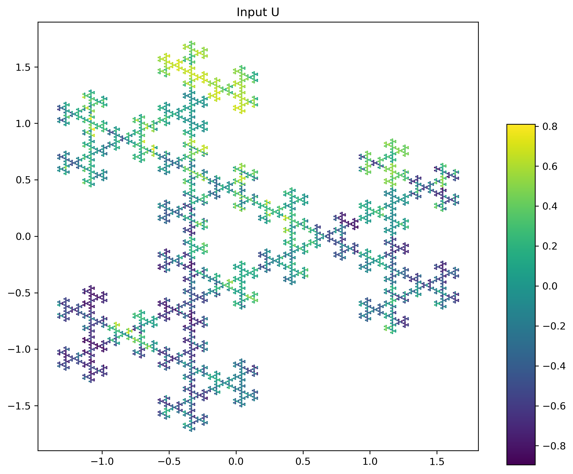
Figure 6. Left side, original image $81\times 81$. Right side, the representation of the image as atest function. We use $p=3$, $L=8$.

References

- [1] S. Albeverio, A. Yu. Khrennikov, V. M. Shelkovich, Theory of -adic distributions: linear and nonlinear models. London Mathematical Society Lecture Note Series, 370. Cambridge University Press, Cambridge, 2010.
- [2] Sergio Albeverio, Andrei Khrennikov, Brunello Tirozzi, -Adic dynamical systems and neural networks, Math. Models Methods Appl. Sci. 9, no. 9 (1999) 1417–1437,.
- [3] V. A. Avetisov, A. Kh. Bikulov, V. A Osipov, -Adic description of characteristic relaxation in complex systems, J. Phys. A 36, no. 15 (2003) 4239–4246.
- [4] V. A. Avetisov, A. H. Bikulov, S. V. Kozyrev, V. A. Osipov, -Adic models of ultrametric diffusion constrained by hierarchical energy landscapes, J. Phys. A 3, no. 2 (2002) 177–189.
- [5] Jenny Benois-Pineau, A. Khrennikov, N. Kotovich, Segmentation of images in -adic and Euclidean metrics, Doklady Mathematics, 64, no. 3 (2001) 450-455.
- [6] Jenny Benois-Pineau, Andrei Khrennikov, Significance delta reasoning with -adic neural networks: application to shot change detection in video, The Computer Journal, 53, no.4 (2010) 417–431.
- [7] Miriam Bocardo-Gaspar, H. García-Compeán, W. A. Zúñiga-Galindo, Regularization of -adic string amplitudes, and multivariate local zeta functions, Lett. Math. Phys. 109, no. 5 (2019) 1167–1204.
- [8] Kristian Bredies, Dirk Lorenz, Mathematical image processing, Applied and Numerical Harmonic Analysis, Birkhäuser/Springer, Cham, 2018.
- [9] Thierry Cazenave, Alain Haraux, An introduction to semilinear evolution equations, Oxford University Press, 1998.
- [10] Leon O. Chua, Lin Yang, Cellular neural networks: theory, IEEE Trans. Circuits and Systems 35, no. 10 (1988) 1257–1272.
- [11] Leon Chua, Lin Yang, Cellular Neural Networks: Applications, IEEE Trans. on Circuits and Systems, 35, no. 10 (1988) 1273-1290.
- [12] Leon O. Chua, Tamas Roska, Cellular neural networks and visual computing: foundations and applications, Cambridge university press, 2002.
- [13] L. O. Chua, CNN: A Paradigm for Complexity, World Scientific Series on Nonlinear Science (Series A), Vol. 31, Singapore: World Scientific Publishing Company, 1998.
- [14] B. Dragovich, A. Yu. Khrennikov, S. V. Kozyrev, I. V. Volovich, On -adic mathematical physics, -Adic Numbers Ultrametric Anal. Appl. 1, no. 1 (2009) 1–17.
- [15] L. Goras, L. Chua, and D. Leenearts, Turing Patterns in CNNs – Part I: Once Over Lightly, IEEE Trans. on Circuits and Systems – I, 42, no. 10 (1995) 602-611.
- [16] L. Goras, L. Chua, and D. Leenearts, Turing Patterns in CNNs – Part II: Equations and Behavior, IEEE Trans. on Circuits and Systems – I, 42, no. 10 (1995) 612-626.
- [17] L. Goras, L. Chua, and D. Leenearts, Turing Patterns in CNNs – Part III: Computer Simulation Results, IEEE Trans. on Circuits and Systems – I, 42, no. 10 (1995) 627-637.
- [18] H. Hua, L. Hovestadt, -Adic numbers encode complex networks, Sci Rep 11, no. 17 (2021). https://doi.org/10.1038/s41598-020-79507-4.
- [19] A. Khrennikov, Information Dynamics in Cognitive, Psychological, Social and Anomalous Phenomena, Springer: Berlin/Heidelberg, Germany, 2004.
- [20] Andrei Yu Khrennikov, Anatoly N. Kochubei, Adic Analogue of the Porous Medium Equation, J Fourier Anal Appl 24 (2018), 1401–1424.
- [21] Andrei Khrennikov, Brunello Tirozzi, Learning of -adic neural networks. Stochastic processes, physics and geometry: new interplays, II (Leipzig, 1999), 395–401, CMS Conf. Proc., 29, Amer. Math. Soc., Providence, RI, 2000.
- [22] Andrei Khrennikov, Sergei Kozyrev, W. A. Zúñiga-Galindo, Ultrametric Equations and its Applications. Encyclopedia of Mathematics and its Applications (168). Cambridge University Press, 2018.
- [23] S. V. Kozyrev, Methods and Applications of Ultrametric and -Adic Analysis: From Wavelet Theory to Biophysics, Sovrem. Probl. Mat., 12, Steklov Math. Inst., RAS, Moscow, (2008) 3–168.
- [24] Neal Koblitz, -adic Numbers, -adic Analysis, and Zeta-Functions, Graduate Texts in Mathematics No. 58, Springer-Verlag, 1984.
- [25] Kochubei A.N., Pseudo-Differential Equations and Stochastics over Non-Archimedean Fields. Marcel Dekker, New York, 2001.
- [26] N.V. Kotovich, A.Yu.Khrennikov, E. L. Borzistaya, Image compression by means of representation by p-adic mappings and approximation by Mahler polynomials, (Russian) Doklady Mathematics, 396, no. 3 (2004) 305–308
- [27] Edwin León-Cardenal, W. A. Zúñiga-Galindo, An introduction to the theory of local zeta functions from scratch, Rev. Integr. Temas Mat. 37 no. 1, (2019) 45–76. https://doi.org/10.18273/revint.v37n12019004.
- [28] Milan Miklavčič, Applied functional analysis and partial differential equations, World Scientific Publishing Co., Inc., River Edge, NJ, 1998.
- [29] Hiroya Nakao, Alexander S. Mikhailov, Turing patterns in network-organized activator-inhibitor systems, Nature Physics 6 (2010), 544-550.
- [30] R. Rammal, R. Toulouse, M. A. Virasoro, Ultrametricity for physicists, Rev. Modern Phys. 58, no. 3, (1986) 765–788.
- [31] Guillermo Sapiro, Geometric partial differential equations and image analysis. Cambridge University Press, Cambridge, 2001.
- [32] Angela Slavova, Cellular neural networks: dynamics and modelling. Mathematical modelling: theory and applications, 16. Kluwer Academic Publishers, Dordrecht, 2003.
- [33] M. H. Taibleson, Fourier analysis on local fields, Princeton University Press, 1975.
- [34] Torresblanca-Badillo Anselmo, Zúñiga-Galindo W. A., Ultrametric diffusion, exponential landscapes, and the first passage time problem, Acta Appl. Math. 157 (2018), 93–116.
- [35] Anselmo Torresblanca-Badillo, W. A. Zúñiga-Galindo, Non-Archimedean pseudodifferential operators and Feller semigroups, Adic Numbers Ultrametric Anal. Appl. 10, no. 1, (2018) 57–73.
- [36] V. S. Vladimirov, I. V. Volovich , E. I. Zelenov , -adic analysis and mathematical physics, World Scientific, 1994.
- [37] B.A. Zambrano-Luna, W.A. Zúñiga-Galindo, -adic Cellular Neural Networks, J Nonlinear Math Phys (2022). https://doi.org/10.1007/s44198-022-00071-8.
- [38] W. A. Zúñiga-Galindo, Non-Archimedean reaction-ultradiffusion equations and complex hierarchic systems, Nonlinearity 3, no. 6, (2018) 2590–2616.
- [39] W. A. Zúñiga-Galindo, Pseudodifferential equations over non-Archimedean spaces. Lectures Notes in Mathematics 2174, Springer, 2016.