Eigen Memory Trees

Abstract

This work introduces the Eigen Memory Tree (EMT), a novel online memory model for sequential learning scenarios. EMTs store data at the leaves of a binary tree and route new samples through the structure using the principal components of previous experiences, facilitating efficient (logarithmic) access to relevant memories. We demonstrate that EMT outperforms existing online memory approaches, and provide a hybridized EMT-parametric algorithm that enjoys drastically improved performance over purely parametric methods with nearly no downsides. Our findings are validated using 206 datasets from the OpenML repository in both bounded and infinite memory budget situations.

1 Introduction

A sequential learning framework (also known as online or incremental learning (Hoi et al., 2021; Losing et al., 2018)) considers a setting in which data instances $x_{t}\in\mathbb{R}^{d}$ arrive incrementally. After each instance, the agent is required to make a decision from a set of $|\mathcal{A}|$ possibilities, $a_{t}\in\mathcal{A}$. The agent then receives scalar feedback $y_{t}$ regarding the quality of the action, and the goal is for the agent to learn a mapping from $x_{t}$ to $a_{t}$ that maximizes the sum of all observed $y_{t}$.

This general paradigm accommodates a wide array of well-studied machine learning scenarios. For example, in online supervised learning, $\mathcal{A}$ is a set of labels—the agent is required to predict a label for each $x_{t}$, and the feedback $y_{t}$, indicates the quality of the prediction.

In a contextual bandit or reinforcement learning setting, $x_{t}$ acts as a context or state, $a_{t}$ is an action, and $y_{t}$ corresponds to a reward provided by the environment. Contextual Bandits have proven useful in a wide variety of settings; their properties are extremely well studied (Langford & Zhang, 2007) and have tremendous theoretical and real-world applications (Bouneffouf et al., 2020).

Regardless of the particulars of the learning scenario, a primary consideration is sample complexity. That is, how can we obtain the highest-performing model given a fixed interaction budget? This often arises when agents only receive feedback corresponding to the chosen action $a_{t}$, i.e. partial feedback. Here, after an interaction with the environment, the agent does not get access to what the best action in hindsight would have been. As a consequence, learners in a partial-feedback setting need to explore different actions even for a fixed $x_{t}$ in order to discover optimal behavior.

Recent work in reinforcement learning has demonstrated that episodic memory mechanisms can facilitate more efficient learning (Lengyel & Dayan, 2007; Blundell et al., 2016; Pritzel et al., 2017; Hansen et al., 2018; Lin et al., 2018; Zhu et al., 2020). Episodic memory (Tulving, 1972) refers to memory of specific past experiences (e.g., what did I have for breakfast yesterday). This is in contrast to semantic memory, which generalizes across many experiences (e.g., what is my favorite meal for breakfast). Semantic memory is functionally closer to parametric approaches to learning, which also rely on generalizations while discarding information about specific events or items.

This paper investigates the use of episodic memory for accelerating learning in sequential problems. We introduce Eigen Memory Trees (EMT), a model that stores past observations in the leaves of a binary tree. Each leaf contains experiences that are somewhat similar to each other, and the EMT is structured such that new samples are routed through the tree based on the statistical properties of previously encountered data. When the EMT is queried with a new observation, this property affords an efficient way to compare it with only the most relevant memories. A learned “scoring” function $w$ is used to identify the most salient memory in the leaf to be used for decision making.

Figure 1: A schematic of the Eigen Memory Tree (EMT) algorithm. The outer boxes indicate the two operations supported by EMT, Learn and Query. The inner boxes show the high-level subroutines that occur to accomplish the outer operation.

Table 1: Cells indicate the number of datasets in which the row algorithm beats the column algorithm with statistical significance. The stacked algorithm we propose (PEMT) has the most wins in each column as indicated by bold.

	PEMT	EMT	PCMT	CMT	Parametric
PEMT	—	167	87	196	110
EMT	31	—	42	177	44
PCMT	4	156	—	192	75
CMT	7	11	10	—	17
Parametric	8	151	10	184	—

Specifically, this work

• introduces the Eigen Memory Tree, an efficient tool for storing, accessing, and comparing memories to current observations (see Figure 1).

• shows that the EMT gives drastically improved performance over comparable episodic memory data structures, and sometimes even outperforms parametric approaches that have no explicit memory mechanism.

• proposes a simple combination EMT-parametric (PEMT) approach, which outperforms both purely parametric and EMT methods with nearly no downsides (see Table 1).

In the following section, we introduce the Eigen Memory Tree and overview the algorithms required for storing and retrieving memories. A schematic of EMT and its high-level algorithms can be seen in Figure 1. With this in mind, Section 3 describes related work.

Section 4 follows with an exhaustive set of experiments, demonstrating the superiority of EMT to previous episodic memory models and motivating the EMT-parametric (PEMT) method, a simple and powerful hybrid strategy for obtaining competitive performance on sequential learning problems. Importantly, we show that the PEMT performance advantage holds even when it is constrained to have a fixed limit on the number of memories it is allowed to store.

All experiments here consider the contextual bandit setting, but EMTs are applicable in broader domains as well. This section continually references Table 1, identifying which methods outperform which other methods by a statistically significant amount over all datasets and replicates. We consider a substantial number of datasets from the OpenML (Vanschoren et al., 2014) repository.

Section 5 summarizes our findings, discusses limitations, and overviews directions for future work.

2 Eigen Memory Tree

As with episodic memory, EMT is structured around storing and retrieving exact memories. We formalize this notion as the self-consistency property: if a memory has been previously $\mathrm{Inserted}$, then a $\mathrm{Query}$ with the same key should return the previously inserted value. The self-consistency property encodes the assumption that the optimal memory to return, if possible, is an exact match for the current observation.

EMT is a memory model with four key characteristics: (1) self-consistency, (2) incremental memory growth, (3) incremental query improvement via supervised feedback, and (4) sub-linear computational complexity with respect to the number of memories in the tree. As we discuss in the literature review below, this combination of characteristics separates EMT from previous approaches.

Memory.

EMT represents memories as a mapping from keys to values, $\mathcal{M}:=\mathbb{R}^{d}\to\mathbb{R}$, where $d$ is the dimensionality of the context $x_{t}$, and $y_{t}\in\mathbb{R}$ corresponds to observed feedback. A query to the EMT requires an $x_{t}$ and returns a previously observed value $\hat{y}\in\mathbb{R}$ from its bank of memories. EMT learning, which updates both the underlying data structure and the scoring mechanism, requires a full $(x_{t},y_{t})$ observation pair $\mathcal{M}$.

Data structure.

The underlying data structure used by the EMT is a binary tree. The tree is composed of a set of nodes, $\mathcal{N}$, each of which is either an internal node or a leaf node. If a node $n\in\mathcal{N}$ is internal it possesses two child nodes ($n.\textrm{left}\in\mathcal{N}$ and $n.\textrm{right}\in\mathcal{N}$), a decision boundary $n.\textrm{boundary}\in\mathbb{R}$, and a top eigenvector $n.\textrm{router}\in\mathbb{R}^{d}$. The decision boundary and top eigenvector, as discussed later, are used to route queries through the tree. If a node $n$ is a leaf node then it will instead possess a finite set of memories $n.\textrm{M}=\left\{(x,y)\in\mathbb{R}^{d}\to\mathbb{R}\right\}$. In addition to the nodes and routers EMT also possesses a single global scoring function responsible for selecting which memory to return given a query and leaf node. This function is parameterised in by the weight vector $w\in\mathbb{R}^{d}$.

Learn.

Newly acquired information is stored during the learning operation (Line 13 in Algorithm 1), which takes an item $\mathcal{M}$ and traverses the tree until a suitable insertion leaf is identified (Line 17 in Algorithm 1). Immediately before insertion, the scoring function weights $w$ are updated such that the scores of the insertion leaf’s memories improve with respect to the observed $x_{t}$ and $y_{t}$ (Line 16 in Algorithm 1)

Algorithm 1 Primary Functions

1:

2:class Node (router$\,\in\mathbb{R}^{d}$, boundary$\,\in\mathbb{R}$, left: Node, right: Node, M$\,\subseteq\mathbb{R}^{d}\times\mathbb{R}$):

3:Initialize: $root\leftarrow$ Node()

4:Initialize: $w\leftarrow$ random vector in $\mathbb{R}^{d}$

5:Initialize: $c\leftarrow$ leaf capacity

6:

7:function Query($x\in\mathbb{R}^{d}$)

8:     $n\leftarrow root$

9:     while $n$ is not leaf $n\leftarrow$ $n.\textrm{left}$ if $\langle n.\textrm{router},x\rangle\leq n.\textrm{boundary}$ else $n.\textrm{right}$

10:     return $\arg\min_{(x_{m},y_{m})\in n.\textrm{M}}$ PredictScorer($x$, $x_{m}$)

11:end function

12:

13:function Learn($x\in\mathbb{R}^{d}$, $y\in\mathbb{R}$)

14:     $n\leftarrow root$

15:     while $n$ is not leaf $n\leftarrow$ $n.\textrm{left}$ if $\langle n.\textrm{router},x\rangle\leq n.\textrm{boundary}$ else $n.\textrm{right}$

16:     UpdateScorer($x$,$y$)

17:     $n.\textrm{M}\leftarrow n.\textrm{M}\cup(x,y)$ $\triangleright$ Insert memory into leaf.

18:     if $|n.\textrm{M}|\geq c$ then

19:         SplitLeaf($n$)

20:     end if

21:end function

Scorer.

EMT’s scorer, $w$, ranks candidate memories at query time. The scorer supports both predictions (see Line 14 Algorithm 2) and updates (see Line 2 Algorithm 2). Intuitively, the scorer can be thought of as a dissimilarity metric, assigning small values to similar query pairs and large values to dissimilar query pairs.

A pair of identical query vectors is guaranteed to result in a score of $0$, satisfying the self-consistency property mentioned earlier. This is achieved for any two $x_{1}$ and $x_{2}$ by applying the scorer on the coordinate-wise absolute value difference between pairs, $z\leftarrow|(x_{1})_{i}-(x_{2})_{i}|\}_{i=1}^{d}$, which is all zeros if the two contexts are identical. Predictions are then made by linearly regressing this vector onto the scorer’s weights, and clipping predictions $\langle w,z\rangle$ such that the minimum is $0$. The clipping operation ensures that predictions will be $0$ even when weights are negative.

Updating the scoring function is done via a ranking loss, which considers (1) $(x_{\textrm{best}},y_{\textrm{best}})$, which is the memory-reward pair that would be retrieved by the scorer currently and (2) $(x_{\textrm{alt}},y_{\textrm{alt}})$, an alternative memory in the same leaf that has a reward most similar to the current observation (omitting the retrieved memory $x_{\textrm{best}}$). If $y_{\textrm{alt}}$ gives a better prediction of the observed reward than $y_{\textrm{best}}$, we adjust the scorer to decrease the learned dissimilarity between $x_{\textrm{alt}}$ and the current target $x_{t}$. Alternatively, if the retrieved memory $y_{\textrm{best}}$ is closer to the observed reward, we do the opposite, emphasizing the similarity between $x_{t}$ and $x_{\textrm{best}}$ and making $x_{t}$ and $x_{\textrm{alt}}$ more dissimilar. Specifically, this is done by taking a gradient step with respect to an $L_{2}$ loss that encourages more similar pairs to have a score near $0$ and more dissimilar pairs to have a score near $1$.

Algorithm 2 Scorer Functions

function UpdateScorer($M\subseteq\mathbb{R}^{d}\times\mathbb{R}$, $x\in\mathbb{R}^{d}$, $y\in R$)

     $(x_{b},y_{b})=\arg\min_{(x_{m},y_{m})\in M}$ PredictScorer($x$,$x_{m}$)

     $(x_{a},y_{a})=\arg\min_{(x_{m},y_{m})\in(M\setminus(x_{b},y_{b}))}|y-y_{m}|$

     if $|y_{b}-y_{t}|<|y_{a}-y_{t}|$ then

         $\mathcal{L}=$PredictScorer($x_{b}$,$x$)${}^{2}+(1-$PredictScorer($x_{a}$,$x$)$)^{2}$

         $w\leftarrow w-\eta\frac{\partial\mathcal{L}}{\partial w}$

     else if $|y_{b}-y_{t}|>|y_{a}-y_{t}|$ then

         $\mathcal{L}=$PredictScorer($x_{a}$,$x$)${}^{2}+(1-$PredictScorer($x_{b}$,$x$)$)^{2}$

         $w\leftarrow w-\eta\frac{\partial\mathcal{L}}{\partial w}$

     end if

end function

function PredictScorer($x_{1}\in\mathbb{R}^{d}$, $x_{2}\in\mathbb{R}^{d}$)

     $z\leftarrow\{|(x_{1})_{i}-(x_{2})_{i}|\}_{i=1}^{d}$ $\triangleright$ $z\in\mathbb{R}^{d}$

     return $\max(0,\langle w,z\rangle)$ $\triangleright$ We clip for self-consistency purposes.

end function

Query.

To predict $y_{t}$ we can call EMT’s $\mathrm{Query}$ operation with $x_{t}$ (see Line 7 in Algorithm 1). Queries to the EMT trigger a search over the internal data structure, beginning at the root node and routing through internal nodes until a leaf is eventually reached. When the search procedure is presented with an internal node $n$, routing follows a simple rule: if $\langle n.\textrm{router},x_{t}\rangle\leq n.\textrm{boundary}$ we proceed left, if not we proceed right (see Line 9 in Algorithm 1). When we arrive at a leaf the scorer is then called to identify the most similar memory available (see Line 10 in Algorithm 1).

Eigen-router initialization.

An important hyperparameter in the EMT is the maximum leaf capacity $c$, which controls the number of memories stored in a single leaf node. Once the leaf reaches this capacity, the corresponding node is assigned a left and right child, and its memories are allocated across them. If $c$ is small, the tree is extended frequently to accommodate new data, and when it is large, the tree grows more slowly. A large $c$ allows many memories to be scored for a particular query, which can improve statistical performance but may damage efficiency. Correspondingly, smaller capacities permit fewer memories to be scored for a given query, which may improve computational efficiency by sacrificing predictive performance.

We check whether a leaf node $n$ is at capacity each time a memory is added to it (i.e., $|n.\textrm{M}|\geq c$). If it is, the leaf is split, turning $n$ into an internal node. The splitting process begins by assigning routing behavior to the node, which governs how new samples will traverse the tree. This is done by (1) approximating the first principal component of its stored memories and (2) computing the median value of memories projected onto this vector. When a new sample arrives, we project it onto this eigenvector and route the sample left if the corresponding value is less than or equal to this median and otherwise route it right (see Line 4 in Algorithm 3).

We follow the same rule for distributing memories across the children of a newly split node—memories with a projection less than or equal to this median are stored in the left child and others are stored in the right. The approximate eigenvector assigned to $n.\textrm{router}$ is computed using Oja’s method, a popular approach for performing PCA on streaming data (Balsubramani et al., 2013) as shown in Algorithm 3. Because the decision boundary $n.\textrm{boundary}$ is the median of the projected memories, the allocation of data across children in a newly split node is nearly even; hopefully resulting in a well-balanced tree.

Algorithm 3 Leaf Functions

function SplitLeaf($n$: Node)

     $n.\textrm{router}\leftarrow$TopEigen($n.\textrm{M}$)

     $n.\textrm{boundary}\leftarrow\textrm{median}(\{\langle n.\textrm{router},x_{m}\rangle|(x_{m},y_{m})\in n.\textrm{M}\})$

     $n.\textrm{left}.\textrm{M}\leftarrow\{(x_{m},y_{m})\in n.\textrm{M}\mid\langle n.\textrm{router},x_{m}\rangle\leq n.\textrm{boundary}\}$

     $n.\textrm{right}.\textrm{M}\leftarrow\{(x_{m},y_{m})\in n.\textrm{M}\mid\langle n.\textrm{router},x_{m}\rangle>n.\textrm{boundary}\}$

     $n.\textrm{M}\leftarrow\emptyset$

end function

function TopEigen($M\subseteq\mathbb{R}^{d}\times\mathbb{R}$)

     $X=\{x_{m}\mid(x_{m},y_{m})\in M\}$ $\triangleright$ $X\in\mathbb{R}^{d\times|M|}$

     $X=X(I_{|M|}-\frac{1}{|M|}\mathbf{1}_{|M|})$ $\triangleright$ Mean center the rows of $X$

     $v\leftarrow$ random unit vector in $\mathbb{R}^{|M|}$

     for $n\leftarrow 1$ to $|M|$ do

         $v\leftarrow\frac{v+\frac{1}{n}(X_{:,n})(X_{:,n})^{\top}v}{||v+\frac{1}{n}(X_{:,n})(X_{:,n})^{\top}v||}$

     end for

     return v

end function

3 Related Work

This section overviews alternative memory structures through the lens of our desiderata: self-consistency, incremental growth, learning, and sub-linear computational complexity. Two illuminating extreme points are associative data structures (e.g., hashmaps) that do not learn and only support exact retrieval; and supervised models (e.g., ordinary least squares) which compile experience into a structure which supports fast retrieval, but cannot guarantee self-consistency.

Classic nearest-neighbor models (Friedman et al., 1975) are self-consistent and grow incrementally, but do not learn (the metric) and have poor computational complexity; considerable attention has unsurprisingly been put towards improving nearest neighbors algorithms along these axes. Exact or approximate nearest-neighbor methods, e.g.,  Beygelzimer et al. (2006); Ram & Sinha (2019); Datar et al. (2004); Dasgupta & Sinha (2013), can reduce computational complexity but (beyond inserting new memories) do not learn. Weinberger et al. (2005) learn a metric for use with nearest-neighbors but does not learn incrementally. Analogously, learned hash functions (Salakhutdinov & Hinton, 2009; Rastegari et al., 2012) produce an associative data structure but learning is not incremental.

Differentiable neural memory systems learn an associative mapping using gradient-based optimization (Sukhbaatar et al., 2015; Graves et al., 2016). Unfortunately their computational demands are severe, preventing practical applications with large memories and prompting variants that use custom hardware (Ni et al., 2019; Ranjan et al., 2019) or exploit sparsity (Karunaratne et al., 2021).

The only memory model in the literature possessing all of EMT’s desiderata is the contextual memory tree (CMT) (Sun et al., 2019). EMT and CMT both use an internal tree structure with routers and a global scorer. EMT differs from CMT in three ways (1) EMT uses fixed top-egeinvector routers while CMT learns routers incrementally, (2) the EMT scorer uses pairwise feature differences rather than CMT’s feature interactions (the importance of this can be seen in our own ablation studies below) and (3) the EMT scorer is updated with respect to a ranking loss function rather than CMT’s squared loss. As discussed later, (1) and (2) together ensure a strong self-consistency constraint, such that exact memories are returned if available. Because CMT updates routing mechanisms, even exact matches for a particular observation may be inaccessible.

Finally, it remains an open question how to best use episodic memory. For example, the work of (Lengyel & Dayan, 2007) evaluates directly using memories to decide how to act in a sequential environment. Other work has used episodic memory as a tool to support a supervised learner either as input into a non-parametric model (Blundell et al., 2016; Pritzel et al., 2017) or as a tool to train a supervised learner (Lin et al., 2018). Still more has treated episodic memory as a complement to supervised learning and the goal is to combine the two model’s predictions Hansen et al. (2018); Feng et al. (2017). Our work evaluates EMT in terms of its performance as a direct predictor (EMT-CB) and as a complementary predictor to a parametric model (PEMT-CB).

4 Experiments

The experiments in this section consider the Contextual Bandit (CB) framework, a setting in which an agent is sequentially presented with a $d$-dimensional “context” vector $x_{t}$ and is required to execute one of $|\mathcal{A}|$ actions. For each executed action $a_{t}\in\mathcal{A}$, the agent receives a corresponding reward $y_{t}$. The goal of the agent is to maximize the total reward received over the course of an evaluation.

The EMT algorithm presented above is a general-purpose supervised learning algorithm, and not an algorithm for solving CB problems specifically. We however can easily adapt EMT for the CB setting by augmenting it with an exploration algorithm (see Algorithm 4). For our experiments we used an $\epsilon$-greedy exploration algorithm with $\epsilon=.1$. That is, on each iteration with probability $\epsilon$ an action in $\mathcal{A}$ was selected with uniform random probability. Otherwise for each $a\in\mathcal{A}$ EMT is queried and the action with the highest predicted reward is taken. We will call this adaptation EMT-CB. Code to reproduce all results is available at https://github.com/pmineiro/memoryrl.

Datasets

We consider $206$ contextual bandit problems derived from OpenML (Vanschoren et al., 2014) supervised classification datasets via a supervised-to-bandit transformation (Bietti et al., 2021). OpenML data are released under a CC-BY license. For large datasets, we consider a random subset of $4,000$ training examples. We also scale the $i$-th feature of every sample $x_{t}^{i}$ in each dataset by $\frac{1}{\max_{t}x_{t}^{i}-\min_{t}x_{t}^{i}}$. For each dataset, the number of available actions $\mathcal{A}$ is equal to the number of classifications available. When the agent correctly classifies a sample it receives a reward equal to one and it receives a reward of zero otherwise.

Evaluation

Learners are evaluated online via progressive loss (Blum et al., 1999). Specifically, each time the agent receives reward, we update the total reward earned, normalized by the total number of interactions. After $T$ total interactions, the progressive reward is $\nicefrac{{1}}{{T}}\sum_{t=0}^{T}y_{t}$. These progressive rewards are plotted throughout the course of this section. Additionally, in order to calculate confidence bounds every data set is evaluated $50$ times with a different random seed for each.

4.1 Self-Consistency

Algorithm 4 Contextual Bandit EMT (EMT-CB)

Initialize: $c$ and $\epsilon$ as desired

function Predict($x_{t}\in\mathbb{R}^{d}$, $\mathcal{A}$)

     With probability $\epsilon$ return uniform random $a\in\mathcal{A}$

     Otherwise return $\arg\max_{a\in\mathcal{A}}$ EMT.Query(($x_{t},a$)

end function

function Learn($x_{t}\in\mathbb{R}^{d}$, $a_{t}\in\mathcal{A}$, $y_{t}\in\mathbb{R}$)

     EMT.Learn(($x_{t}$, $a_{t}$), $y_{t}$)

end function

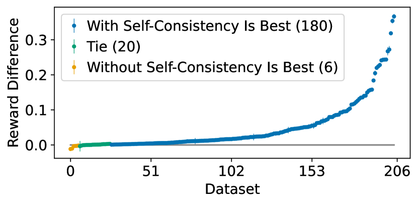
Figure 2: A per-dataset comparison of final progressive reward between EMT and a variant of EMT that does not include self-consistency. Each point corresponds to a single dataset, and the vertical axis shows the difference between the two learners. The horizontal axis is ordered by this performance difference.

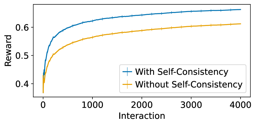
Figure 3: Progressive reward for EMT-CB and a variant of EMT-CB without forced self-consistency, where each line corresponds to an average over all $206$ datasets in the OpenML repository. Progressive reward is shown as a function of environment interactions and vertical lines are standard error.

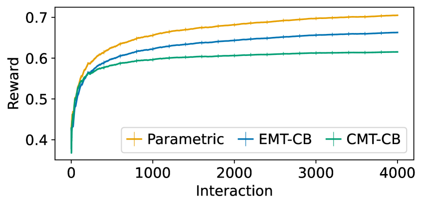
Figure 4: A progressive reward comparison between EMT-CB and parametric, where each line corresponds to an average over $168$ datasets in the OpenML repository. Reward is shown as a function of the number of environment interactions and vertical lines denote standard error. Parametric actually outperforms EMT on average, which we address with the hybridized algorithm discussed in Section 4.4.

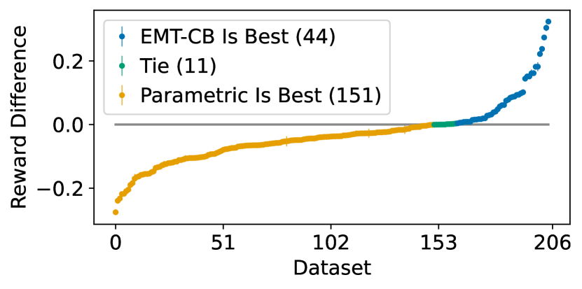
Figure 5: A per-dataset comparison of final progressive reward between EMT-CB and parametric. Each point corresponds to a single dataset, and the vertical axis shows the difference between the two learners. The horizontal axis is ordered by this performance difference. Here we see that while there are many datasets for which parametric does better, there are $44$ datasets where EMT is higher performing.

The EMT incorporates two particular design decisions: (1) using eigenvector routing and (2) using a scorer where self-consistency is a hard constraint, which as mentioned earlier, guarantees that an exact-match memory is always retrieved as long as one is available.

To examine the importance of self-consistency, we compare EMT to a variant that does not include this property. In this variant, we modify Line 15 of Algorithm 2 such that the input to the regressor, $z$, is the interaction of features in samples $x_{1}$ and $x_{2}$, instead of a dimension-wise difference. As a consequence, it is not the case that $\langle w,z\rangle$ is guaranteed to be zero for identical samples.

Figure 3 compares the performance of these algorithms on a dataset-by-dataset basis. The plotted points show the difference in total progressive reward averaged over random seeds. The plot shows that in $180$ of the $206$ datasets considered, self-consistency provides significant improvements. In the remaining $6$ the performance difference is negligible.

Figure 3 compares the average progressive reward for these two algorithms over $168$ datasets, with respect to the number of training examples. The number of datasets is slightly smaller here because we omit datasets with fewer than $4,000$ training examples. We can see that the self-consistent version has significantly better performance over all interactions on average.

4.2 Comparison To Alternative Episodic Memory Data Structures

The most natural comparison to EMT is, as mentioned earlier, Contextual Memory Trees. The CMT implementation used throughout this work for CMT-CB is the official Vowpal Wabbit (VW) (Langford et al., 2007) implementation published by Sun et al. (2019). It is also worth noting that the original CMT paper evaluated the performance of CMT in an online framework with full-feedback, meaning that the agent receives information about the correct answer for each $x_{t}$ it encounters. In the partial-feedback scenarios studied here, where the agent only receives information corresponding to the executed action, we find CMT is far less performant overall.

Specifically, our results demonstrate that EMT’s differences in routing and scoring endow it with performance superior to CMT in bandit scenarios. We see this both in terms of performance over time (Figure 5) and total performance on individual datasets (Table 1 and Appendix Figure 5) where EMT soundly outperforms CMT. This plot also compares to a parametric algorithm discussed in the proceeding section.

4.3 Comparison to Parametric Model

Another natural comparison for this analysis is between EMT-CB and a parametric CB learner. A parametric approach could be thought of as encoding semantic memories, focusing on high-level concepts rather than specific experiences.

The parametric model is a linear regressor, taking context-action features as inputs and predicting expected rewards. The model is trained using SGD on the squared loss, as implemented by VW. Like EMT-CB and CMT-CB, this model is $\epsilon$-greedy, selecting uniform random actions with probability $\epsilon$ and selecting the action that yields the highest predicted reward with probability $1-\epsilon$. We use VW’s default hyperparameter values (including $\epsilon=.1$) along with 1st and 2nd-order polynomial features. Table 1 and Figure 5 shows that EMT beats the parametric model on $44$ cases (a minority).

The results here are reminiscent of the “no free lunch” theorem (Wolpert & Macready, 1997) which states there is no one universal learner that wins in all problems. Rather we must try and determine the most appropriate learner for each circumstance. The following subsection proposes a simple and high-performing method that is able to combine parametric and EMT-CB with almost no downsides.

To understand the dataset qualities that result in EMT-CB outperforming the parametric approach, we conducted a thorough meta-analysis, which is provided in Appendix 6. We find that the qualities most predictive of whether EMT will outperform parametric are (1) the mutual information between samples and labels and (2) how well the top eigenvector explains dataset variance. Intuitively, the former could be thought of as how reasonable it is to compare a new sample with the data stored at its corresponding leaf and the latter could be thought of as how reasonable it is for EMT to aggregate leaf samples based on the first principle component.

4.4 Comparison of Stacked to Parametric

Due to the mixed results of EMT-CB when compared against the parametric algorithm, we propose a simple method to combine the two learners, which we call PEMT-CB (and PCMT-CB when applying this method to CMT-CB). This combination is a simple stacking approach (Wolpert, 1992) where the rewards for each action predicted by EMT-CB are passed to the parametric CB model as a single additional feature. The parametric learner has no idea the additional feature came from EMT-CB and treats it simply as an additional parameter to optimize via SGD.

Figure 6 shows that PEMT-CB is able to outperform the parametric model on $110$ individual datasets and under-performs by a very small margin in only $8$ datasets. It is worth noting that stacking two learners in a partial feedback setting is more challenging than in a full-feedback setting because both learners may have different data needs for learning and not all actions can be explored. Previous work has sought to explicitly address this challenge from a statistical perspective (Agarwal et al., 2017), but here we find the simple stacking approach to be surprisingly powerful.

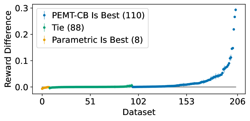
Figure 6: A per-dataset comparison of final progressive reward between PEMT-CB and parametric. Each point corresponds to a single dataset, and the vertical axis shows the difference between the two learners. The horizontal axis is ordered by this performance difference. PEMT-CB almost always performs at least as well as the parametric approach.

4.5 Bounded memory analysis

For our final analysis we examine how sensitive EMT is to a memory budget, limiting the amount of memories EMT is permitted to keep. In order to maintain this limit we use a simple least-recently-used (LRU) strategy to eject a memory whenever our memory budget is exceeded. To get a sense of how the loss of memories might impact performance over time we filter our datasets down to the $116$ which have $32,000$ or more training examples and evaluate out to $32,000$ iterations rather than the $4,000$ explored up to this point.

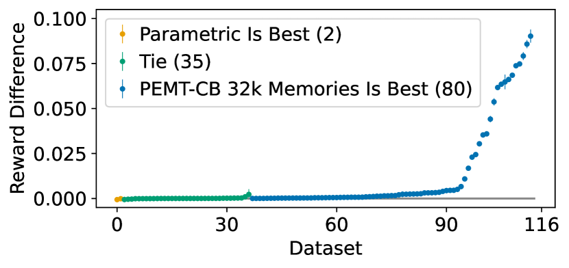
Figure 14: A progressive reward comparison with varying amounts of memory budgets. Each line corresponds to an average over 116 datasets in the OpenML repository. Reward is a function of the number of environment inter-actions and vertical lines denote standard error.

We find that even with a budget of $1,000$ memories (with memory eviction via LRU) PEMT-CB still outperformed parametric alone with statistical significance on $61$ datasets (see Appendix Figure 14 and 14). Figure 7 shows that a $16,000$-sample memory budget works almost exactly as well as the no-budget version of PEMT-CB. That is, equivalent performance can be attained despite the fact that the memory can only hold half as much information. Even when using an extremely conservative memory budget of $1,000$ samples, PEMT-CB only accrues a loss in reward of $.0075$ on average. Overall, very few memories are needed to consistently beat the parametric approach in isolation, and not much is needed to match the performance of the unbounded memory variant of PEMT-CB.

5 Discussion and future directions

Summary

As discussed in Section 3, finding methods that effectively use episodic memory is an important and active area of research. This work proposes a new episodic memory model for sequential learning called Eigen Memory Trees (EMT). EMT possesses four distinguishing characteristics: (1) self-consistency, (2) incremental growth, (3) incremental learning, and (4) sub-linear computational complexity. EMT adds to an important but somewhat understudied area in online learning: efficient, online memory models.

To evaluate the effectiveness of EMT we converted $206$ datasets from OpenML into contextual bandit problems. Using these we compared EMT’s performance to an alternative online memory model, CMT, and a parametric CB learner. EMT outperformed CMT across the board (see Figure 5) while outperforming parametric in $44$ of the $206$ (see Figure 5) datasets.

We further proposed PEMT-CB, a simple extension of EMT that is able to consistently outperform both EMT and parametric alone, even when forced to use a small memory budget (see Table 1). The aggregate strategy passes EMT reward predictions as a feature into the parametric learner. This result is important for a number of reasons. First, it suggests that EMT offers a no-downside method for improving existing CB algorithms. Second, to our knowledge, this is the first work demonstrating that stacking can improve performance in the partial feedback setting of contextual bandits (cf. (Agarwal et al., 2017)).

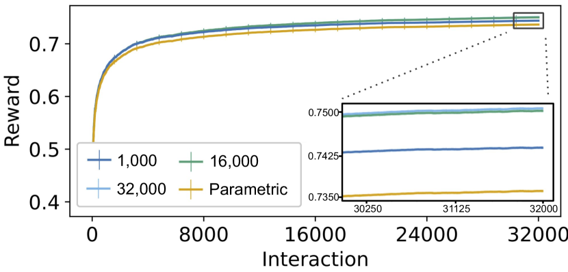
Figure 7: The performance loss between the unbounded PEMT-CB and bounded PEMT-CB algorithms is minimal even with a 3.1% memory budget. Additionally, at no budget level does PEMT-CB performance drop below the parametric model. Each line corresponds to an average over 116 datasets in the OpenML repository. Reward is a function of the number of environment inter-actions and vertical lines denote standard error.

Applied machine learning models often have to work with resources constrained by business and operational requirements. For memory models this is often the amount of memories that can be stored and efficiently accessed. We evaluated PEMT-CB performance for four memory budgets, showing that observed performance improvements of PEMT-CB are largely maintained even with an extremely constrained memory capacity (see Figure 7). Perhaps most importantly, constraining the memory budget had no negative impact on the performance of the parametric learner.

Applications, limitations and future studies

The fast reactivity of memorization, when appropriate, is appealing in real world applications where data acquisition incurs natural costs via acting in the world. Thus, incorporating memorization into practical systems could broaden the applicability of contextual bandits, e.g., to scenarios in information retrieval and dialogue systems (Bouneffouf et al., 2020).

EMT also seems especially well suited for quick-changing environments. Rather than requiring multiple SGD steps to update, new memories are immediately accessible after insertion, and stale memories can be directly removed or added when situations change in known ways. This highlights both a limitation of this study as well as an opportunity: how robust is EMT to non-stationarity? The fixed nature of EMT’s top-eigen routers along with our simple LRU eviction rule for memory budgeting likely make the model susceptible to performance degradation when environments shift.

Appendix

6 Meta-Data analysis

An analysis was performed to understand the characteristics of the datasets where EMT-CB outperformed the parametric CB learner. Twelve dataset features were selected from the meta-learning literature. These twelve features are described in Table 2.

Table 2: The features used to analyze why EMT outperformed the parametric learner on some datasets.

Feature	Reference	Description
Top Eigenvector Explained		The percentage of dataset variance explained by the top eigenvector.
Eigenvector Count To Explain 95% Var	Lorena et al. (2019)	The number of eigenvectors required to explain 95% of the feature variance.
Mean Mutual Information Feature/Label	Castiello et al. (2005); Reif et al. (2014)	The average amount of mutual information between each feature and the target label.
1 Nearest Neighbor Accuracy	Reif et al. (2014); Abdelmessih et al. (2010)	The accuracy of a 1 nearest neighbors classifier on the dataset.
Single Node Decision Tree Accuracy	Reif et al. (2014); Abdelmessih et al. (2010)	The accuracy of a single node decision tree on the dataset.
Naive Bayes Accuracy	Reif et al. (2014); Abdelmessih et al. (2010)	The accuracy of a naive Bayes classifier on the dataset.
Normed Label Entropy	Lorena et al. (2019); Castiello et al. (2005); Reif et al. (2014)	The amount of entropy in the class distribution (normed so that 1 is maximum entropy).
Noise to Signal Ratio	Castiello et al. (2005)	Ratio extra feature entropy to mutual information between features and labels.
Binary Feature Count		The count of the number of binary features in the dataset. For one hot encoded categorical features this counts every level.
Percent of Nonzero Features	Lorena et al. (2019)	The percentage of non-zero features in the dataset.
Efficiency of Best Single Feature	Lorena et al. (2019)	A measure of the single best feature’s ability to distinguish classes. The efficiency is averaged across all one-v-one label matchups.
Maximum Fisher’s Discriminant Ratio	Lorena et al. (2019)	A Measure of feature overlap when discriminating class labels. The ratio is averaged across all one-v-one label match-ups.

We trained a random forest (RF) model using the features in Table 2 to predict when EMT would outperform the parametric learner. This model was able to predict winning CB model with a macro f1 score of .82 on held-out datasets. Figure 11 shows the average reduction in Gini impurity for each feature.

We then trained a compact RF model to see the minimum features needed. We used repeated k-fold cross validation with feature selection applied to the training split before fitting our RF model. The final reduced model had an f1 score of .79 on held out data using only 3 features: percent of variance explained by the top eigenvector, percent of nonzero features, average amount of mutual information between features and labels (measured in bits). We now look at these more closely.

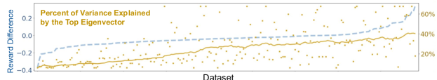
Figure 8: This plot visualizes the relationship between the variance explained by the top-eigenvector for a dataset and the performance of EMT-CB versus parametric. The x-axis represents our study datasets. The blue line shows the difference in performance between EMT-CB and parametric. The yellow points show the feature values for each dataset and the yellow line show the rolling average of all the yellow points.

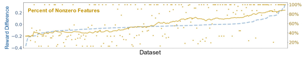
Figure 9: This plot visualizes the relationship between the percent of nonzero features in a dataset and and the performance of EMT-CB versus parametric. The x-axis represents our study datasets. The blue line shows the difference in performance between EMT-CB and parametric. The yellow points show the feature values for each dataset and the yellow line show the rolling average of all the yellow points.

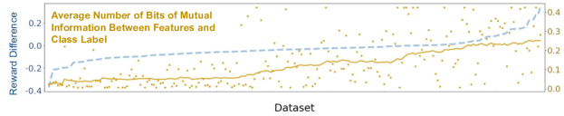
Figure 10: This plot visualizes the relationship between the mutual information metadata feature and the performance of EMT-CB vs parametric. The x-axis represents our study datasets. The blue line shows the difference in performance between EMT-CB and parametric. The yellow points show the feature values for each dataset and the yellow line show the rolling average of all the yellow points.

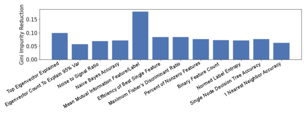
Figure 11: The average decrease in impurity in an RF model predicting whether EMT outperforms parametric.

The first of these features measures the explanatory power of the top eigenvector. We can see that this has a positive correlation with the performance of memory in Figure 8. We believe these datasets with a more informative top eigenvector for the whole dataset likely have more informative top eigenvector routers leading to improved tree searches for the EMT.

The second of these features is the percentage of non-zero values in a dataset. For this feature we observed that the fewer non-zero features in a dataset the better EMT performed (see Figure 9). When we looked at datasets with a high percentage of zero values the most common cause were large amounts of one hot encoded categorical features. Categorical variables with a large number of levels are naturally difficult to compare via a metric since each level is equidistant from every other level. In this case learning an effective scorer would become very challenging parametric would have a greater chance of beating EMT-CB.

The final feature in our compact model was the mutual information between individual features and a dataset’s class (see Figure 10). This is a non-normalized value so datasets with more labels and fewer non-zero features will likely have higher values of this feature. For example, a dataset with a binary label has an upper limit of $1$ for this feature while a dataset with $30$ class labels has an upper limit of $4.91$. High values in this variable also indicate that there is a strong statistical relationship between features and class labels but place no restriction on the functional that relationship may take.

7 Supplementary Figures

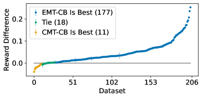
Figure 12: A per-dataset comparison of final progressive reward. Each point corresponds to a single dataset. The y-axis shows the difference between the two learners. The x-axis is ordered by this performance difference.

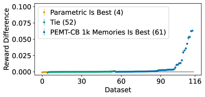
Figure 13: A progressive reward comparison with varying amounts of memory budgets. Each line corresponds to an average over 116 datasets in the OpenML repository. Reward is a function of the number of environment interactions and vertical lines denote standard error.

References

- Abdelmessih et al. (2010) Sarah Daniel Abdelmessih, Faisal Shafait, Matthias Reif, and Markus Goldstein. Landmarking for meta-learning using rapidminer. In RapidMiner community meeting and conference. Citeseer, 2010.
- Agarwal et al. (2017) Alekh Agarwal, Haipeng Luo, Behnam Neyshabur, and Robert E Schapire. Corralling a band of bandit algorithms. In Conference on Learning Theory, pp. 12–38. PMLR, 2017.
- Balsubramani et al. (2013) Akshay Balsubramani, Sanjoy Dasgupta, and Yoav Freund. The fast convergence of incremental pca. In C.J. Burges, L. Bottou, M. Welling, Z. Ghahramani, and K.Q. Weinberger (eds.), Advances in Neural Information Processing Systems, volume 26. Curran Associates, Inc., 2013. URL https://proceedings.neurips.cc/paper/2013/file/c913303f392ffc643f7240b180602652-Paper.pdf.
- Beygelzimer et al. (2006) Alina Beygelzimer, Sham Kakade, and John Langford. Cover trees for nearest neighbor. In Proceedings of the 23rd international conference on Machine learning, pp. 97–104, 2006.
- Bietti et al. (2021) Alberto Bietti, Alekh Agarwal, and John Langford. A contextual bandit bake-off. Journal of Machine Learning Research, 22(133):1–49, 2021.
- Blum et al. (1999) Avrim Blum, Adam Kalai, and John Langford. Beating the hold-out: Bounds for k-fold and progressive cross-validation. In Proceedings of the twelfth annual conference on Computational learning theory, pp. 203–208, 1999.
- Blundell et al. (2016) Charles Blundell, Benigno Uria, Alexander Pritzel, Yazhe Li, Avraham Ruderman, Joel Z Leibo, Jack Rae, Daan Wierstra, and Demis Hassabis. Model-free episodic control, 2016.
- Bouneffouf et al. (2020) Djallel Bouneffouf, Irina Rish, and Charu Aggarwal. Survey on applications of multi-armed and contextual bandits. In 2020 IEEE Congress on Evolutionary Computation (CEC), pp. 1–8, 2020. doi: 10.1109/CEC48606.2020.9185782.
- Castiello et al. (2005) Ciro Castiello, Giovanna Castellano, and Anna Maria Fanelli. Meta-data: Characterization of input features for meta-learning. In International Conference on Modeling Decisions for Artificial Intelligence, pp. 457–468. Springer, 2005.
- Dasgupta & Sinha (2013) Sanjoy Dasgupta and Kaushik Sinha. Randomized partition trees for exact nearest neighbor search. In Conference on learning theory, pp. 317–337. PMLR, 2013.
- Datar et al. (2004) Mayur Datar, Nicole Immorlica, Piotr Indyk, and Vahab S Mirrokni. Locality-sensitive hashing scheme based on p-stable distributions. In Proceedings of the twentieth annual symposium on Computational geometry, pp. 253–262, 2004.
- Feng et al. (2017) Yang Feng, Shiyue Zhang, Andi Zhang, Dong Wang, and Andrew Abel. Memory-augmented neural machine translation. arXiv preprint arXiv:1708.02005, 2017.
- Friedman et al. (1975) Jerome H Friedman, Forest Baskett, and Leonard J Shustek. An algorithm for finding nearest neighbors. IEEE Transactions on computers, 100(10):1000–1006, 1975.
- Graves et al. (2016) Alex Graves, Greg Wayne, Malcolm Reynolds, Tim Harley, Ivo Danihelka, Agnieszka Grabska-Barwińska, Sergio Gómez Colmenarejo, Edward Grefenstette, Tiago Ramalho, John Agapiou, et al. Hybrid computing using a neural network with dynamic external memory. Nature, 538(7626):471–476, 2016.
- Hansen et al. (2018) Steven Hansen, Alexander Pritzel, Pablo Sprechmann, Andre Barreto, and Charles Blundell. Fast deep reinforcement learning using online adjustments from the past. In S. Bengio, H. Wallach, H. Larochelle, K. Grauman, N. Cesa-Bianchi, and R. Garnett (eds.), Advances in Neural Information Processing Systems, volume 31. Curran Associates, Inc., 2018. URL https://proceedings.neurips.cc/paper/2018/file/f7bdb0e100275600f9e183e25d81822d-Paper.pdf.
- Hoi et al. (2021) Steven CH Hoi, Doyen Sahoo, Jing Lu, and Peilin Zhao. Online learning: A comprehensive survey. Neurocomputing, 459:249–289, 2021.
- Karunaratne et al. (2021) Geethan Karunaratne, Manuel Schmuck, Manuel Le Gallo, Giovanni Cherubini, Luca Benini, Abu Sebastian, and Abbas Rahimi. Robust high-dimensional memory-augmented neural networks. Nature communications, 12(1):1–12, 2021.
- Langford & Zhang (2007) John Langford and Tong Zhang. The epoch-greedy algorithm for multi-armed bandits with side information. In J. Platt, D. Koller, Y. Singer, and S. Roweis (eds.), Advances in Neural Information Processing Systems, volume 20. Curran Associates, Inc., 2007.
- Langford et al. (2007) John Langford, Lihong Li, and Alex Strehl. Vowpal wabbit online learning project, 2007.
- Lengyel & Dayan (2007) Máté Lengyel and Peter Dayan. Hippocampal contributions to control: The third way. In J. Platt, D. Koller, Y. Singer, and S. Roweis (eds.), Advances in Neural Information Processing Systems, volume 20. Curran Associates, Inc., 2007. URL https://proceedings.neurips.cc/paper/2007/file/1f4477bad7af3616c1f933a02bfabe4e-Paper.pdf.
- Lin et al. (2018) Zichuan Lin, Tianqi Zhao, Guangwen Yang, and Lintao Zhang. Episodic memory deep q-networks. In Proceedings of the Twenty-Seventh International Joint Conference on Artificial Intelligence, IJCAI-18, pp. 2433–2439. International Joint Conferences on Artificial Intelligence Organization, 7 2018. doi: 10.24963/ijcai.2018/337. URL https://doi.org/10.24963/ijcai.2018/337.
- Lorena et al. (2019) Ana C Lorena, Luís PF Garcia, Jens Lehmann, Marcilio CP Souto, and Tin Kam Ho. How complex is your classification problem? a survey on measuring classification complexity. ACM Computing Surveys (CSUR), 52(5):1–34, 2019.
- Losing et al. (2018) Viktor Losing, Barbara Hammer, and Heiko Wersing. Incremental on-line learning: A review and comparison of state of the art algorithms. Neurocomputing, 275:1261–1274, 2018.
- Ni et al. (2019) Kai Ni, Xunzhao Yin, Ann Franchesca Laguna, Siddharth Joshi, Stefan Dünkel, Martin Trentzsch, Johannes Müller, Sven Beyer, Michael Niemier, Xiaobo Sharon Hu, et al. Ferroelectric ternary content-addressable memory for one-shot learning. Nature Electronics, 2(11):521–529, 2019.
- Pritzel et al. (2017) Alexander Pritzel, Benigno Uria, Sriram Srinivasan, Adrià Puigdomènech Badia, Oriol Vinyals, Demis Hassabis, Daan Wierstra, and Charles Blundell. Neural episodic control. In Doina Precup and Yee Whye Teh (eds.), Proceedings of the 34th International Conference on Machine Learning, volume 70 of Proceedings of Machine Learning Research, pp. 2827–2836. PMLR, 06–11 Aug 2017. URL https://proceedings.mlr.press/v70/pritzel17a.html.
- Ram & Sinha (2019) Parikshit Ram and Kaushik Sinha. Revisiting kd-tree for nearest neighbor search. In Proceedings of the 25th acm sigkdd international conference on knowledge discovery & data mining, pp. 1378–1388, 2019.
- Ranjan et al. (2019) Ashish Ranjan, Shubham Jain, Jacob R Stevens, Dipankar Das, Bharat Kaul, and Anand Raghunathan. X-mann: A crossbar based architecture for memory augmented neural networks. In Proceedings of the 56th Annual Design Automation Conference 2019, pp. 1–6, 2019.
- Rastegari et al. (2012) Mohammad Rastegari, Ali Farhadi, and David Forsyth. Attribute discovery via predictable discriminative binary codes. In European Conference on Computer Vision, pp. 876–889. Springer, 2012.
- Reif et al. (2014) Matthias Reif, Faisal Shafait, Markus Goldstein, Thomas Breuel, and Andreas Dengel. Automatic classifier selection for non-experts. Pattern Analysis and Applications, 17(1):83–96, 2014.
- Salakhutdinov & Hinton (2009) Ruslan Salakhutdinov and Geoffrey Hinton. Semantic hashing. International Journal of Approximate Reasoning, 50(7):969–978, 2009.
- Sukhbaatar et al. (2015) Sainbayar Sukhbaatar, Jason Weston, Rob Fergus, et al. End-to-end memory networks. Advances in neural information processing systems, 28, 2015.
- Sun et al. (2019) Wen Sun, Alina Beygelzimer, Hal Daumé Iii, John Langford, and Paul Mineiro. Contextual memory trees. In Kamalika Chaudhuri and Ruslan Salakhutdinov (eds.), Proceedings of the 36th International Conference on Machine Learning, volume 97 of Proceedings of Machine Learning Research, pp. 6026–6035. PMLR, 09–15 Jun 2019.
- Tulving (1972) Endel Tulving. Episodic and semantic memory. In Endel Tulving and Wayne Donaldson (eds.), Organization of memory, pp. 381–402. Academic Press, Oxford, England, 1972.
- Vanschoren et al. (2014) Joaquin Vanschoren, Jan N Van Rijn, Bernd Bischl, and Luis Torgo. Openml: networked science in machine learning. ACM SIGKDD Explorations Newsletter, 15(2):49–60, 2014.
- Weinberger et al. (2005) Kilian Q Weinberger, John Blitzer, and Lawrence Saul. Distance metric learning for large margin nearest neighbor classification. Advances in neural information processing systems, 18, 2005.
- Wolpert (1992) David H Wolpert. Stacked generalization. Neural networks, 5(2):241–259, 1992.
- Wolpert & Macready (1997) David H Wolpert and William G Macready. No free lunch theorems for optimization. IEEE transactions on evolutionary computation, 1(1):67–82, 1997.
- Zhu et al. (2020) Guangxiang Zhu, Zichuan Lin, Guangwen Yang, and Chongjie Zhang. Episodic reinforcement learning with associative memory. In International Conference on Learning Representations, 2020. URL https://openreview.net/forum?id=HkxjqxBYDB.